Calibration of an airborne HO_x instrument using the All Pressure Altitude-based Calibrator for HO_x Experimentation (APACHE)

Laser-induced fluorescence (LIF) is a widely used technique for both laboratory-based and ambient atmospheric chemistry measurements. However, LIF instruments require calibrations in order to translate instrument response into concentrations of chemical species. Calibration of LIF instruments measuring OH and HO₂ (HO_x) typically involves the photolysis of water vapor by 184.9 nm light, thereby producing quantitative amounts of OH and HO₂. For ground-based HO_x instruments, this method of calibration is done at one pressure (typically ambient pressure) at the instrument inlet. However, airborne HO_x instruments can experience varying cell pressures, internal residence times, temperatures, and humidity during flight. Therefore, replication of such variances when calibrating in the lab is essential to acquire the appropriate sensitivities. This requirement resulted in the development of the APACHE (All Pressure Altitude-based Calibrator for HO_x Experimentation) chamber to characterize the sensitivity of the airborne LIF-FAGE (fluorescence assay by gas expansion) HO_x instrument, HORUS, which took part in an intensive airborne campaign, OMO-Asia 2015. It utilizes photolysis of water vapor but has the additional ability to alter the pressure at the nozzle of the HORUS instrument. With APACHE, the HORUS instrument sensitivity towards OH (26.1–7.8 cts s⁻¹ pptv⁻¹ mW⁻¹, ±22.6 % 1σ; cts stands for counts by the detector) and HO₂ (21.2–8.1 cts s⁻¹ pptv⁻¹ mW⁻¹, ±22.1 % 1σ) was characterized to the external pressure range at the instrument nozzle of 227–900 mbar. Measurements supported by a computational fluid dynamics model, COMSOL Multiphysics, revealed that, for all pressures explored in this study, APACHE is capable of initializing a homogenous flow and maintaining near-uniform flow speeds across the internal cross section of the chamber. This reduces the uncertainty regarding average exposure times across the mercury (Hg) UV ring lamp. Two different actinometrical approaches characterized the APACHE UV ring lamp flux as $\mathrm{6.37}\times {\mathrm{10}}^{\mathrm{14}}(\pm \mathrm{1.3}\times {\mathrm{10}}^{\mathrm{14}}$) photons cm⁻² s⁻¹. One approach used the HORUS instrument as a transfer standard in conjunction with a calibrated on-ground calibration system traceable to NIST standards, which characterized the UV ring lamp flux to be $\mathrm{6.9}(\pm \mathrm{1.1})\times {\mathrm{10}}^{\mathrm{14}}$ photons cm⁻² s⁻¹. The second approach involved measuring ozone production by the UV ring lamp using an ANSYCO O3 41 M ozone monitor, which characterized the UV ring lamp flux to be $\mathrm{6.11}(\pm \mathrm{0.8})\times {\mathrm{10}}^{\mathrm{14}}$ photons cm⁻² s⁻¹. Data presented in this study are the first direct calibrations of an airborne HO_x instrument, performed in a controlled environment in the lab using APACHE.

1 Introduction

It is well known that the hydroxyl (OH) radical is a potent oxidizing agent in daytime photochemical degradation of pollutants sourced from anthropogenic and biogenic processes, thus accelerating their removal from our atmosphere. The hydroperoxyl radical (HO₂) also plays a central role in atmospheric oxidation as it not only acts as a reservoir for OH but is involved in formation of other oxidants such as peroxides and impacts the cycling of pollutants such as NO_x ($=\mathrm{NO}+{\mathrm{NO}}_{\mathrm{2}}$) (Lelieveld et al., 2002). Therefore, measurements of OH and HO₂ (HO_x) within the troposphere are essential in understanding the potential global-scale impacts of pollutants in both the present day and in climate predictions. One common HO_x measurement method is laser-induced fluorescence (LIF) (Stevens et al., 1994; Brune et al., 1995; Hard et al., 1995; Martinez et al., 2003; Faloona et al., 2004; Stone et al., 2010; Hens et al., 2014; Novelli et al., 2014). Other methods have been successfully implemented to measure HO_x. Chemical ionization mass spectrometry (CIMS) (Cantrell et al., 2003; Mauldin et al., 2004; Sjostedt et al., 2007; Dusanter et al., 2008; Kukui et al., 2008; Albrecht et al., 2019) and differential optical absorption spectroscopy (DOAS) (Brauers et al., 1996, 2001; Schlosser et al., 2007) have also been used in the measurement of HO_x in the field and in intercomparison projects with LIF instrumentation. However, low atmospheric concentrations of HO_x (Schlosser et al., 2009) and potential interferences (Faloona et al., 2004; Fuchs et al., 2011, 2016; Mao et al., 2012; Hens et al., 2014; Novelli et al., 2014) can make HO_x measurements especially challenging. Airborne LIF-FAGE (LIF–fluorescence assay by gas expansion) instruments experience large variability in pressure, humidity, instrument internal air density, and internal quenching during flights, which cause a wide array of instrumental sensitivities (Faloona et al., 2004; Martinez et al., 2010; Regelin et al., 2013; Winiberg et al., 2015). Therefore, it is critical to utilize a calibration system that can suitably reproduce in-flight conditions to determine the instrument response to known levels of OH and HO₂ to acquire robust HO_x measurements.

The first stage of the Hydroxyl Radical measurement Unit based on fluorescence Spectroscopy (HORUS) inlet is an inlet preinjector (IPI), used to determine the concentration of background OH interferences by removing atmospheric OH from the signal via addition of an OH scavenger such as propane. IPI draws 50–230 sL min⁻¹ depending on altitude and is susceptible to temperature- and pressure-driven changes in internal reaction rates and residence times under flight conditions. This has implications for the removal of atmospheric OH in the inlet and for the characterization of background interference signals in HORUS. Therefore, a device capable of providing stable high flows while reproducing a wide range of pressures and temperatures is needed in order to calibrate the airborne HORUS instrument. This led to the production, characterization, and utilization of the calibration device APACHE (All Pressure Altitude-based Calibrator for HO_x Experimentation) which is described in depth in this work.

2 Experimental design and setup

2.1 APACHE design overview

Figure 1 shows the overview of the APACHE system. In front of the APACHE inlet, a series of mixing blocks are installed where multiple dry synthetic air additions are injected into a controlled humidified air supply ensuring thorough mixing of water vapor before being measured by a LI-COR 6262 CO₂∕H₂O (Fig. 1a). This air is then fed into a large mass flow controller (MFC). The construction of the APACHE chamber itself is shown in Fig. 1b. The first section contains the diffuser inlet with a sintered filter (bronze alloy, Amtag, filter class 10). This 2 mm thick sintered filter, with a pore size of 35 µm, initializes a homogeneous flow and further improves the mixing of water vapor in front of the UV ring lamp (described further in Sect. 4). The water photolysis section contains a low-pressure, 0.8 A, mercury ring lamp (uv-technik; see Fig. S1 in the Supplement) which produces a constant radial photon flux at 184.9 nm, situated 133 mm after the sintered filter and separated from the main APACHE chamber by an airtight quartz window. Between the lamp and the quartz window there is an anodized aluminum band with thirty 8 mm apertures blocking all light apart from that going through the apertures, which reduces the amount of UV flux entering APACHE and limits the size of the illuminated area. The IPI system is clamped down 169.5 mm behind the photolysis section in such a way that the instrument sample flow is perpendicular to the airflow passing over the IPI nozzle. The nozzle protrudes 51.5 mm into the APACHE cavity much like it is when installed in the aircraft shroud system (see Fig. 2), and it is made airtight with the use of O-rings. Opposite the IPI nozzle, there is an airtight block attachment containing a series of monitoring systems. A pitot tube attached to an Airflow PTSX-K 0-10Pa differential pressure sensor (accuracy rating of 1 % at full scale, 1σ) is used to monitor the internal flow speeds within APACHE. A 3 kΩ NTC-EC95302V thermistor is used to monitor the air temperature, and an Edwards ASG2-1000 pressure sensor (with an accuracy rating of ±4 mbar, 2σ) monitors the static air pressure. Additionally, there are two 1∕4 in. (6.35 mm) airtight apertures in the monitoring block that can be opened to enable other instrumentation to be installed.

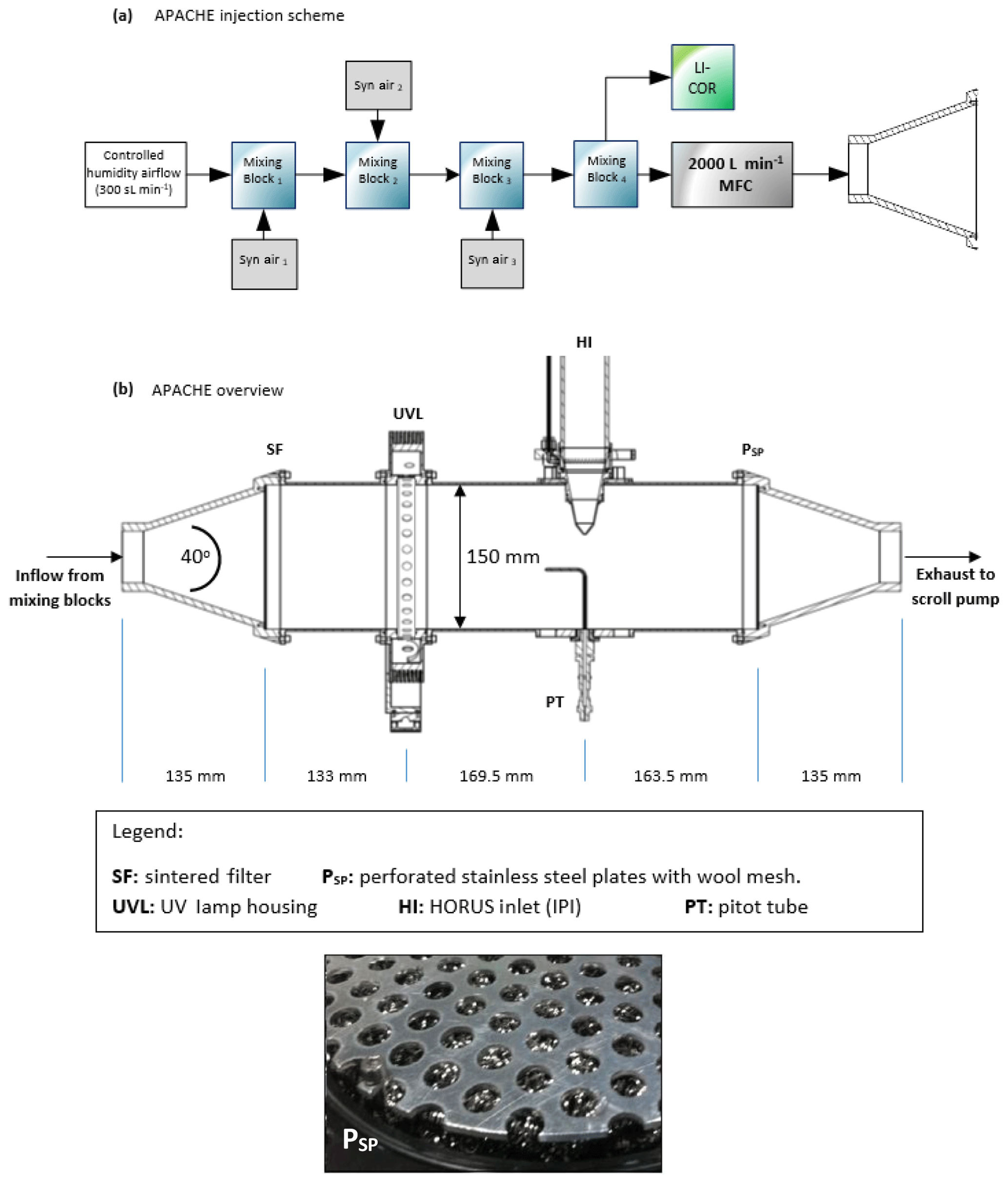
Figure 1 Overview of the APACHE system and the premixing setup used in the lab to calibrate the HORUS airborne instrument. A picture at the bottom shows the perforated stainless-steel plates with wool mesh.

2.2 Pressure control

For this study, the operational pressure range of APACHE used was 227–900 mbar, with a precision of ±0.1 % (1σ) and accuracy of ±2 % (1σ) and with mass flows ranging from 200 to 990 sL min⁻¹ (sL stands for standard liter). This was achieved using an Edwards GSX160 scroll pump controlling the volume flow in combination with a MFC (Bronkhorst F-601A1-PAD-03-V) controlling the mass flow of air entering APACHE. This system reached air speeds of 0.9 to 1.5 m s⁻¹ through APACHE at pressures ranging from 250 to 900 mbar and at temperatures ranging from 282 to 302 K. Temperature changes inside APACHE are not controlled. However, as air temperature is measured throughout the calibration device and HORUS, any term that is affected by temperature is characterized using the corresponding measured temperature values. Although not critical for this study, the operational pressure range of APACHE can be extended by changing the draw speed of the Edwards scroll pump. However, that may cause the flow speeds and potentially the flow speed profiles across the UV ring lamp to vary in between different pressure calibrations.

2.3 The airborne HORUS instrument

The LIF-FAGE instrument developed by our group (HORUS) is based on the original design of GTHOS (Ground-based Tropospheric Hydrogen Oxides Sensor) described by Faloona et al. (2004) and is described in further detail by Martinez et al. (2010). The airborne instrument is a revised and altered design to perform under conditions experienced during flight and conform to aeronautical regulations. It was primarily developed for installation on the High Altitude and Long Range Research Aircraft (HALO) and took place in the OMO-Asia 2015 airborne campaign. The system comprises of an external inlet shroud, detections axes, a laser system, and a vacuum system (Fig. 2). Additionally, this is the first airborne LIF-FAGE instrument measuring HO_x with a dedicated inlet preinjector (IPI) system installed for the purpose of removing atmospheric OH, enabling real-time measurements and quantification of potential chemical background OH interferences, OH−CHEM (Mao et al., 2012). The airborne IPI system is redesigned to fit within the shroud inlet system, and its walls are heated to 30 ^∘C, while maintaining similar operational features to the on-ground IPI installation (Novelli et al., 2014). To prevent excessive collisions of OH and HO₂ with the IPI nozzle and internal walls, thus limiting losses of HO_x during flight, the momentum inertia of the air passing through the external shroud system had to be overcome to promote flow direction into the instrument. This was achieved by installing a choke point behind the IPI nozzle in the inlet shroud, resulting in a reduction in airflow speed. For example without the shroud choke, flow speeds in excess of 200 m s⁻¹ could occur in the shroud during flight. However, with the choke point, flow speeds in the shroud during flight did not exceed 21 m s⁻¹ during OMO-Asia 2015, which is sufficiently below the sample velocities of IPI during flight (44–53 m s⁻¹). Additionally, it limits nonparallel flows across the IPI nozzle created by variable pitch, roll, and yaw changes of the aircraft. As the aircraft changes pitch, roll, and yaw, the measured OH variability increases by $\pm \mathrm{4.51}\times {\mathrm{10}}^{\mathrm{4}}$ cm⁻³ (1σ), which is only 10 % to 15 % higher than the natural variability of OH. This increase in variability is negligible as is represents, depending on internal pressure, 19 % to 30 % of the detection limit of the instrument. Both of these effects of the external shroud improve the measurement performance by reducing variable wall losses of HO_x at the IPI nozzle under flight conditions. The IPI system (with a nozzle orifice diameter of 6.5 mm) samples (51 to 230 sL min⁻¹) from the central airflow moving through the internal shroud. A critical orifice is located at the end of IPI in the center of the IPI cross section, which enables the HORUS instrument to sample (3 to 17 sL min⁻¹) from the central flow moving through IPI. This further reduces influences of wall loss within IPI on the overall measured signal in the cells. The removal of excess flow moving through IPI occurs via a perforated ring that surrounds the base of the critical orifice cone, evacuated by a blower.

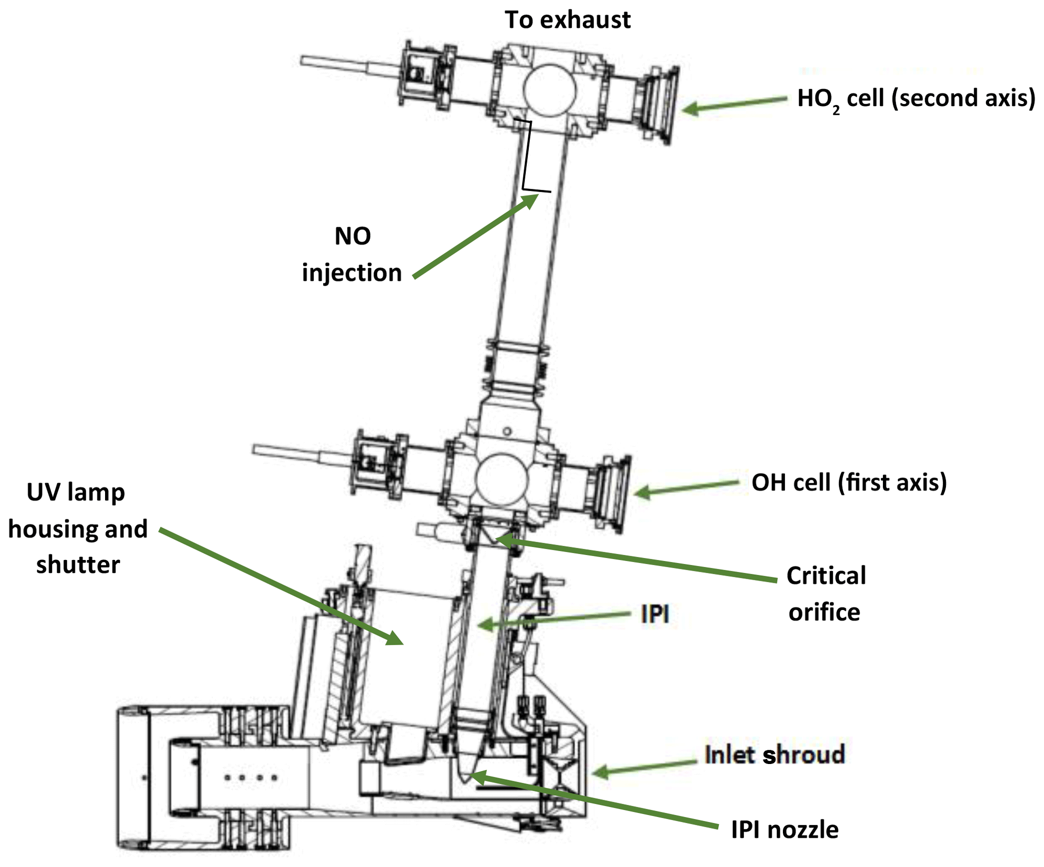
Figure 2 Overview of the airborne HORUS system as installed in the HALO aircraft. HO₂ is measured indirectly through the addition of NO that quantitatively converts HO₂ into OH. The NO injection occurs via a stainless-steel 1∕8 in. (3.175 mm) line, shaped into a ring perpendicular to the airflow with several unidirectional apertures of 0.25 mm diameter creating essentially a NO shower.

As with other LIF-FAGE HO_x instruments, HORUS measures an off-resonance signal to discern the net OH fluorescence signal. This is achieved by successive cycling of the laser tuning from on-resonance (measuring the total signal of OH fluorescence and the signal originating from other fluorescence and electronic sources) to off-resonance (measuring all the above except the OH fluorescence). The HORUS instrument utilizes the Q₁(2) transition $X^{\mathrm{2}}{\mathrm{\Pi }}_{\mathrm{3}/\mathrm{2}}(v{}^{\prime \prime }=\mathrm{0})\to A^{\mathrm{2}}{\mathrm{\Sigma }}^{+}(v{}^{\prime }=\mathrm{0}$) (Freeman, 1958; Dieke and Crosswhite, 1962; Langhoff et al., 1982; Dorn et al., 1995; Holland et al., 1995; Mather et al., 1997). The net OH signal (S_OH) is the difference between the on-resonance and off-resonance signals, OH-WAVE (Mao et al., 2012). The OH sensitivity (C_OH) and average laser power within the detection axis ($W_{z_{\mathrm{1}\mathrm{pwr}}}$) are then used to calculate the absolute OH mixing ratio (see Eq. 1). HO₂ is measured indirectly through the quantitative conversion of atmospheric HO₂ to OH by injection of nitric oxide (NO) under the low-pressure conditions within HORUS.

$$\begin{array}{}\text{(R1)}& {\mathrm{HO}}_{\mathrm{2}}+\mathrm{NO}\to {\mathrm{NO}}_{\mathrm{2}}+\mathrm{OH}.\end{array}$$

When NO is injected into the instrument, both ambient OH and HO₂ are measured in the second detection axis. The net HO₂ signal ($S_{{\mathrm{HO}}_{\mathrm{2}}}$) in the second axis is therefore derived from subtracting the net OH signal from the first detection axis normalized by the ratio of the OH sensitivities for the two detection axes (C_OH(2)∕C_OH) from the net HO_x signal ($S_{{\mathrm{HO}}_x}$). Then $S_{{\mathrm{HO}}_{\mathrm{2}}}$ is corrected by the sensitivity to HO₂ ($C_{{\mathrm{HO}}_{\mathrm{2}}})$ and laser power ($W_{z_{\mathrm{2}\mathrm{pwr}}}$) to reach the absolute HO₂ mixing ratio (see Eq. 2).

$$\begin{array}{}\text{(1)}& {\displaystyle }\left[\mathrm{OH}\right]={\displaystyle \frac{S_{\mathrm{OH}}}{\left(C_{\mathrm{OH}}\cdot W_{z_{\mathrm{1}\mathrm{pwr}}}\right)}},\text{(2)}& {\displaystyle }\begin{array}{rl}\left[{\mathrm{HO}}_{\mathrm{2}}\right]& ={\displaystyle \frac{\mathrm{1}}{\left(C_{{\mathrm{HO}}_{\mathrm{2}}}\cdot W_{z_{\mathrm{2}\mathrm{pwr}}}\right)}}\\ & \cdot \left\{S_{{\mathrm{HO}}_x}-{\displaystyle \frac{\left(C_{\mathrm{OH}\left(\mathrm{2}\right)}\cdot W_{z_{\mathrm{2}\mathrm{pwr}}}\right)}{\left(C_{\mathrm{OH}}\cdot W_{z_{\mathrm{1}\mathrm{pwr}}}\right)}}{S}_{\mathrm{OH}}\right\},\end{array}\end{array}$$

where $W_{z_{\mathrm{1}\mathrm{pwr}}}$ is the laser power in the first detection axis, $W_{z_{\mathrm{2}\mathrm{pwr}}}$ is the laser power in the second detection axis, and C_OH and $C_{{\mathrm{HO}}_{\mathrm{2}}}$ are the calibrated sensitivity factors for OH and HO₂ (cts s⁻¹ pptv⁻¹ mW⁻¹) respectively. By calibrating using a known OH mixing ratio, the instrument sensitivity C_OH can be determined by rearranging Eq. (1) to

$$\begin{array}{}\text{(3)}& C_{\mathrm{OH}\left(\mathrm{cal}\right)}=S_{{\mathrm{OH}}_{\left(\mathrm{cal}\right)}}/\left(\left[\mathrm{OH}\right]\cdot W_{z_{\mathrm{1}\mathrm{pwr}}}\right).\end{array}$$

The sensitivity of HORUS depends on the internal pressure, water vapor mixing ratios, and temperature, which are subject to change quite significantly during flight. Therefore, further parameterization when calibrating is required to fully constrain the sensitivity response of the instrument at various flight conditions. Equation (4) shows the terms that affect the sensitivity of the first HORUS axis that measures OH.

$$\begin{array}{}\text{(4)}& \begin{array}{rl}& C_{\mathrm{OH}}\left(P,T\right)=\text{c0}\cdot {\mathit{\rho }}_{\mathrm{Int}}\left(P,T\right)\cdot Q_{\mathrm{IF}}\left(P,T,{\mathrm{H}}_{\mathrm{2}}\mathrm{O}\right)\cdot b_{\mathrm{c}}\left(T\right)\\ & \cdot \left[{\mathit{\alpha }}_{\mathrm{IPI}}\left(P,T\right)\cdot {\mathit{\alpha }}_{\mathrm{HORUS}}\left(P,T\right)\right],\end{array}\end{array}$$

where c0 is determined by calibrations and is the lump sum coefficient of all the pressure-independent factors affecting the HORUS sensitivity, for example, OH absorption cross section at 308 nm, the photon collection efficiency of the optical setup and quantum yield of the detectors, and pressure-independent wall loss effects. For calibrations, c0 is normalized by laser power and has the units cts pptv⁻¹ s⁻² cm³ molecule⁻¹ mW⁻¹. ρ_Int is the internal molecular density. Q_IF is the quenching effect(s), which consists of the natural decay frequency of OH; OH decay due to collisional quenching that is dependent on pressure, temperature, and water vapor mixing ratio; and the detector opening and closing gating times after the initial excitation laser pulse. Both are pressure-dependent terms as denoted in Eq. (4). The Boltzmann correction (b_c) has a temperature dependency as it corrects for any OH molecules that enter the HORUS instrument in a thermally excited state and are therefore not measurable by fluorescence excitation at the wavelength used. α is the pressure-dependent OH transmission, which is the fraction of OH that reaches the point of detection. This term is separated for the two-tier pressure conditions present in the instrument. The term α_IPI represents the correction for pressure- and temperature-dependent OH loss on the walls within IPI. The term α_HORUS is the correction for pressure-dependent OH loss to the walls within the HORUS detection axes post critical orifice. While the quenching effects, internal densities, and Boltzmann corrections can be quantified by calculation, and the power entering the measurement cell is measured, the two factors that need to be determined through calibration are c0 and OH transmission, α. Once the c0 coefficient and α terms are known, the final in-flight-measured OH mixing ratio (pptv) is found:

$$\begin{array}{}\text{(5)}& \left[\mathrm{OH}\right]=S_{\mathrm{OH}}/\left(\text{c0}\cdot {\mathit{\rho }}_{\mathrm{Int}}\cdot Q_{\mathrm{IF}}\cdot b_{\mathrm{c}}\cdot \left[{\mathit{\alpha }}_{\mathrm{IPI}}\cdot {\mathit{\alpha }}_{\mathrm{HORUS}}\right]\cdot W_{z_{\mathrm{1}\mathrm{pwr}}}\right).\end{array}$$

As S_OH scales with laser power, the terms that describe the instrument sensitivity shown as the denominator in Eq. (5), which ultimately have the units cts s⁻¹ pptv⁻¹ mW⁻¹, must also be scaled to the measured laser power ($W_{z_{\mathrm{1}\mathrm{pwr}}}$) during flight to acquire the absolute measurement of OH mixing ratio. As depicted in both Figs. 1b and 2, the complete system is calibrated with IPI attached and operating as it did when installed in the aircraft. Therefore, the combined losses of OH within IPI and in the low-pressure regime post critical orifice (that has a diameter of 1.4 mm) contribute to the overall calibrated C_OH sensitivity factor in the same way during measurement and calibrations, meaning that the OH transmission of HORUS can be quantified with both OH transmission terms (α_IPI and α_HORUS) combined into one term (α_Total).

$$\begin{array}{}\text{(6)}& \left[\mathrm{OH}\right]=S_{\mathrm{OH}}/\left(\text{c0}\cdot {\mathit{\rho }}_{\mathrm{Int}}\cdot Q_{\mathrm{IF}}\cdot b_{\mathrm{c}}\cdot \left[{\mathit{\alpha }}_{\mathrm{Total}}\right]\cdot W_{z_{\mathrm{1}\mathrm{pwr}}}\right)\end{array}$$

Figure 3 shows the schematic of the different factors described above and their impact on the overall sensitivity.

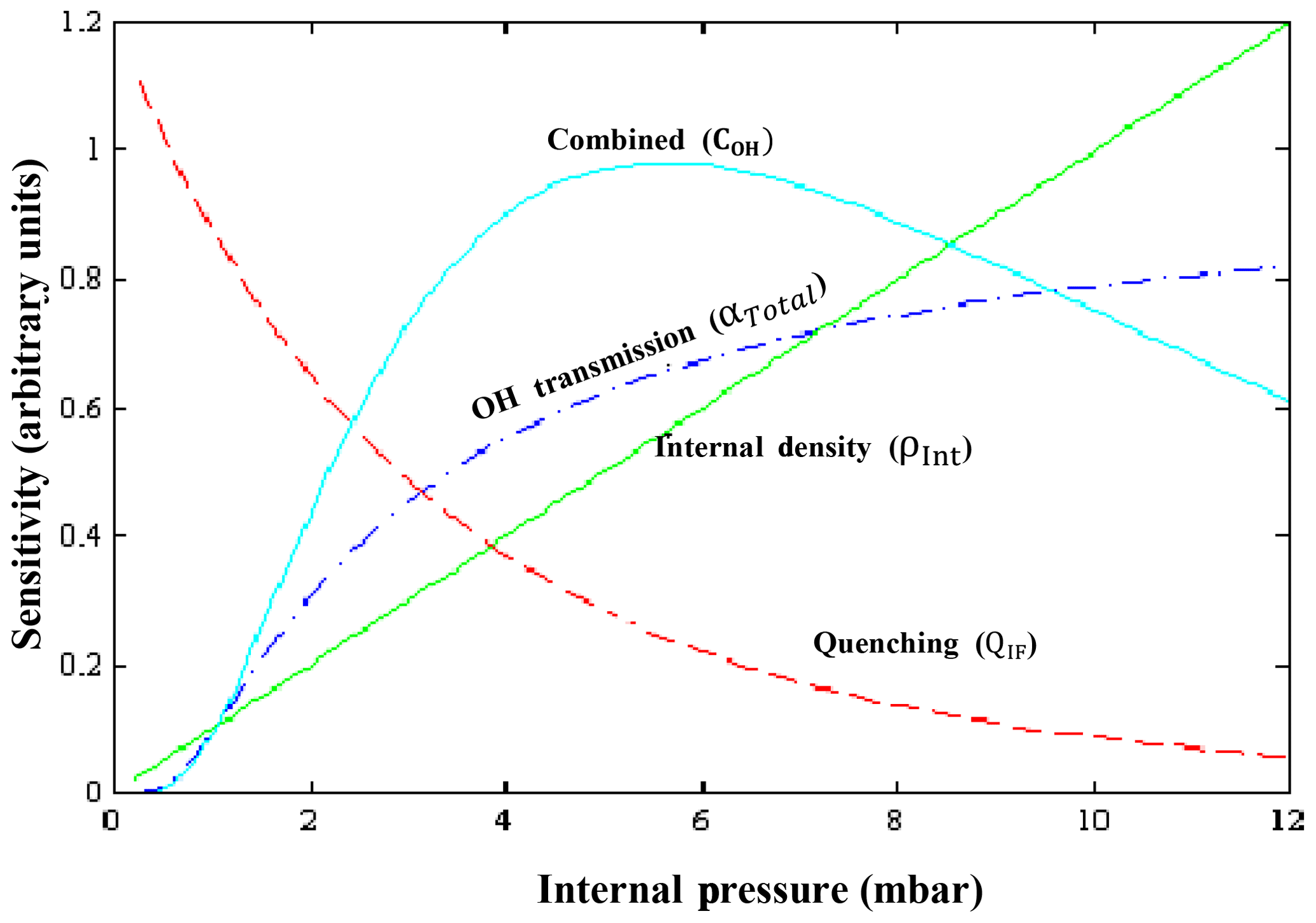
Figure 3 A schematic showing the overall sensitivity curve as a function of internal pressure (light blue line), OH transmission (dotted–dashed dark blue line), internal density (green line), and the quenching (dashed red line).

3 Calibration method and theory

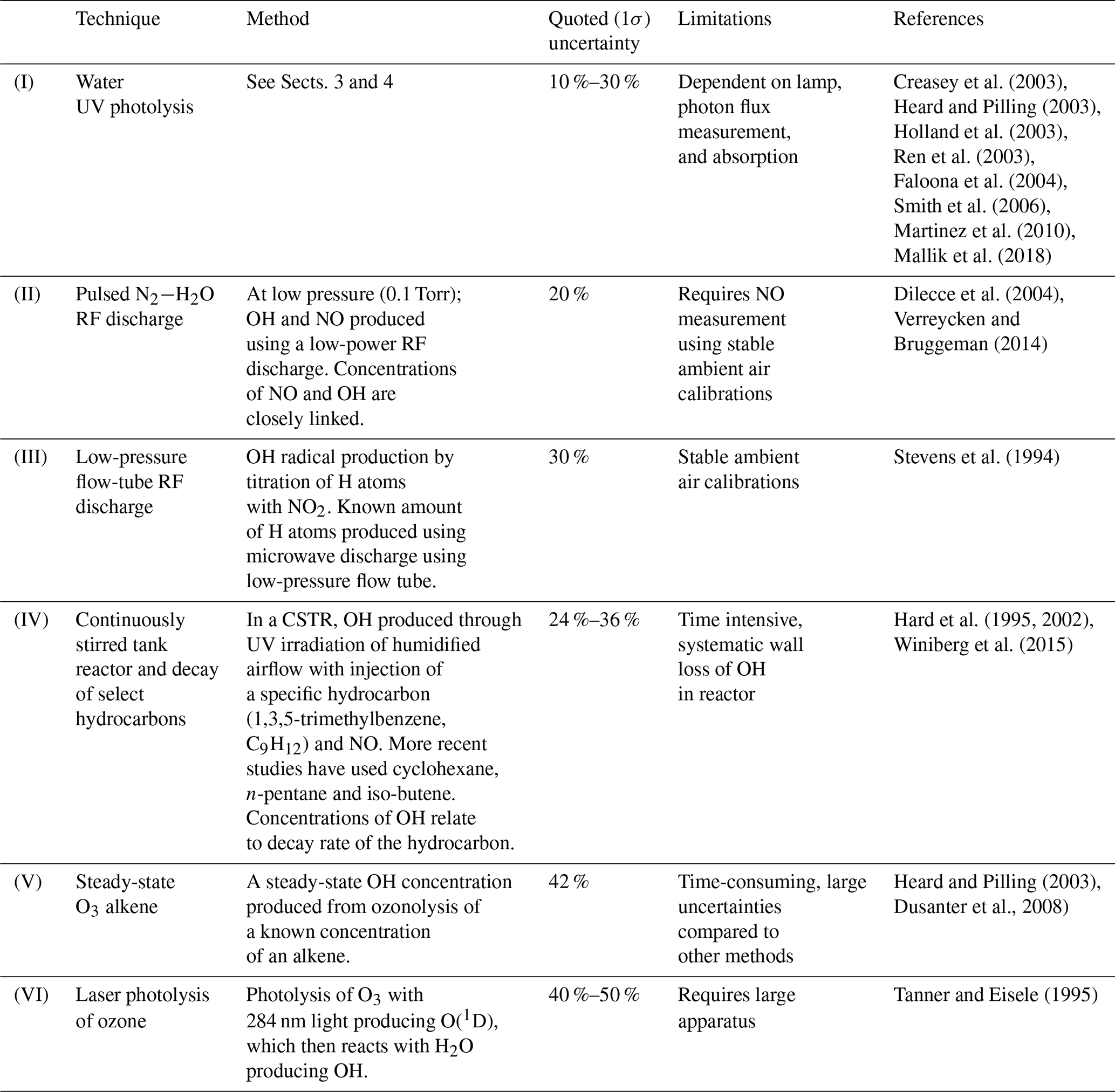
As an overview, Table 1 shows common calibration techniques for OH instruments. The APACHE system is based on the production of known quantified and equal concentrations of OH and HO₂ via photolysis of water vapor in only synthetic air using a Hg ring lamp emitting UV radiation at 184.9 nm.

$$\begin{array}{}\text{(R2)}& {\displaystyle }& {\displaystyle }{\mathrm{H}}_{\mathrm{2}}\mathrm{O}+h\mathit{\upsilon }\stackrel{\mathit{\lambda }=\mathrm{184.9}\mathrm{nm}}{⟶}\mathrm{OH}+{\mathrm{H}}^{*}\text{(R3)}& {\displaystyle }& {\displaystyle }{\mathrm{H}}^{*}+{\mathrm{O}}_{\mathrm{2}}\stackrel{{\mathrm{O}}_{\mathrm{2}}}{⟶}\mathrm{OH}+{\mathrm{O}}_{\mathrm{3}}\text{(R4)}& {\displaystyle }& {\displaystyle }{\mathrm{H}}^{*}\stackrel{M}{⟶}\mathrm{H}\text{(R5)}& {\displaystyle }& {\displaystyle }\mathrm{H}+{\mathrm{O}}_{\mathrm{2}}\stackrel{M}{⟶}{\mathrm{HO}}_{\mathrm{2}}\end{array}$$

Stable water mixing ratios with a variability of <2 % were achieved by heating 300 sL min⁻¹ flow of synthetic air to 353 K and introducing deionized water using a peristaltic pump into this heated gas flow, causing it to evaporate before entering a 15 L mixing chamber. This prevents recondensation and humidity spikes when the pump is introducing the water. The humidified gas flow is then diluted (to around 3 mmol mol⁻¹) and mixed further with additional dry pure synthetic air via a series of mixing blocks to achieve the required and desired stable water vapor mixing ratios. The photolysis of H₂O has only one spin-allowed and energetically viable dissociation channel at 184.9 nm (Engel et al., 1992), meaning the quantum yields of OH and H^* are unified (Sander et al., 2003). Even though Reaction (R3) is possible particularly since the H^* atoms can carry transitional energies of 0.7 eV at 189.4 nm (Zhang et al., 2000), the fast removal of energy by Reaction (R4) allows for the general assumption that all H^* atoms produced lead to HO₂ production (Fuchs et al., 2011). The use of water photolysis as a OH and HO₂ radical source for calibration of HO_x instruments has been adopted in a number of studies (Heard and Pilling, 2003; Ren et al., 2003; Faloona et al., 2004; Dusanter et al., 2008; Novelli et al., 2014; Mallik et al., 2018). As an example, the factors required to quantify the known concentrations of OH and HO₂ during calibrations are shown below:

$$\begin{array}{}\text{(7)}& \left[\mathrm{OH}\right]=\left[{\mathrm{HO}}_{\mathrm{2}}\right]=\left[{\mathrm{H}}_{\mathrm{2}}\mathrm{O}\right]\cdot {\mathit{\sigma }}_{{\mathrm{H}}_{\mathrm{2}}\mathrm{O}}\cdot F_{\mathrm{184.9}\mathrm{nm}}\cdot {\mathit{\varphi }}_{{\mathrm{H}}_{\mathrm{2}}\mathrm{O}}\cdot t,\end{array}$$

where in Eq. (7) the OH and HO₂ concentrations are a product of photolysis of a known concentration of water vapor [H₂O], and ${\mathit{\sigma }}_{{\mathrm{H}}_{\mathrm{2}}\mathrm{O}}$ is the absorption cross section of water vapor, $\mathrm{7.22}(\pm \mathrm{0.22})\times {\mathrm{10}}^{-\mathrm{20}}$ cm² per molecule at 184.9 nm (Hofzumahaus et al., 1997; Creasey et al., 2000). F_184.9 nm is the actinic flux (photons cm⁻² s⁻¹) of the mercury lamp used for photolysis, ${\mathit{\varphi }}_{{\mathrm{H}}_{\mathrm{2}}\mathrm{O}}$ is the quantum yield, and t is exposure time. The quantum yield of water vapor photolysis at the 184.9 nm band is 1 (Creasey et al., 2000).

Table 1 Various known methods for OH instrument calibrations. CSTR stands for continuously stirred tank reactor.

4 Results and discussion

4.1 Flow conditions

With any calibration device, the flow conditions must be characterized to inform subsequent methods and calibrations. Regarding APACHE, the two main factors to be resolved are (i) how uniform the flow speed profiles and therefore exposure times in respect to the APACHE cross section are and (ii) the impact of OH wall losses.

To this end, experimental and model tests were performed to determine whether the combination of the sintered filter as well as the stainless-steel perforated plates and wool arrangement could provide a homogeneous flow. This means that under operation the flow speeds should be uniform along the cross section of APACHE to within the uncertainty of the measurements. This is to ensure that the air masses passing across the lamp have the same exposure times irrespective of where they are in the cross section. Additionally, model simulations can provide an indication of, as a function of APACHE pressure, the development and scale of boundary air conditions where air parcels experience extended contact time with the interior walls of APACHE and so have pronounced OH wall losses. This highlights potential flow conditions where there is sufficient time between the photolysis zone and the IPI nozzle to allow APACHE boundary air to expand into and influence the OH content of the air being sampled by HORUS.

4.1.1 Flow speed profiles

During calibration, the pressures within the HORUS instrument had to be controlled and monitored to replicate the in-flight conditions. The APACHE chamber pressure is equivalent to the in-flight pressure in the shroud where the HORUS system samples. The pressure of the detection axes depends on the pressure at the IPI nozzle and the efficiency of the pumps. Within IPI itself, the airflow through it is dependent on the pressure gradient between the shroud and the ambient pressure at the IPI exhaust or alternatively the APACHE pressure and pressure in front of the XDS35 scroll pump (post IPI blower). During the campaign, the exhausts of all blowers and pumps of the HORUS system were attached to the passive exhaust system of the aircraft and were thus exposed to ambient pressure. Therefore, the same IPI blower and pumps that were installed on HALO were used in the lab, and throughout the calibrations the pressure at the exhaust for every blower and pumps involved in the HORUS instrument was matched to the respective in-flight ambient pressures by attaching a separate pressure sensor, needle valve, and XDS35 scroll pump system. Additionally, to match the power that is provided on the aircraft, a three-phase mission power supply unit was used to power the pumps in the lab during testing and throughout the calibrations. Figure 4 shows the lab setup described above.

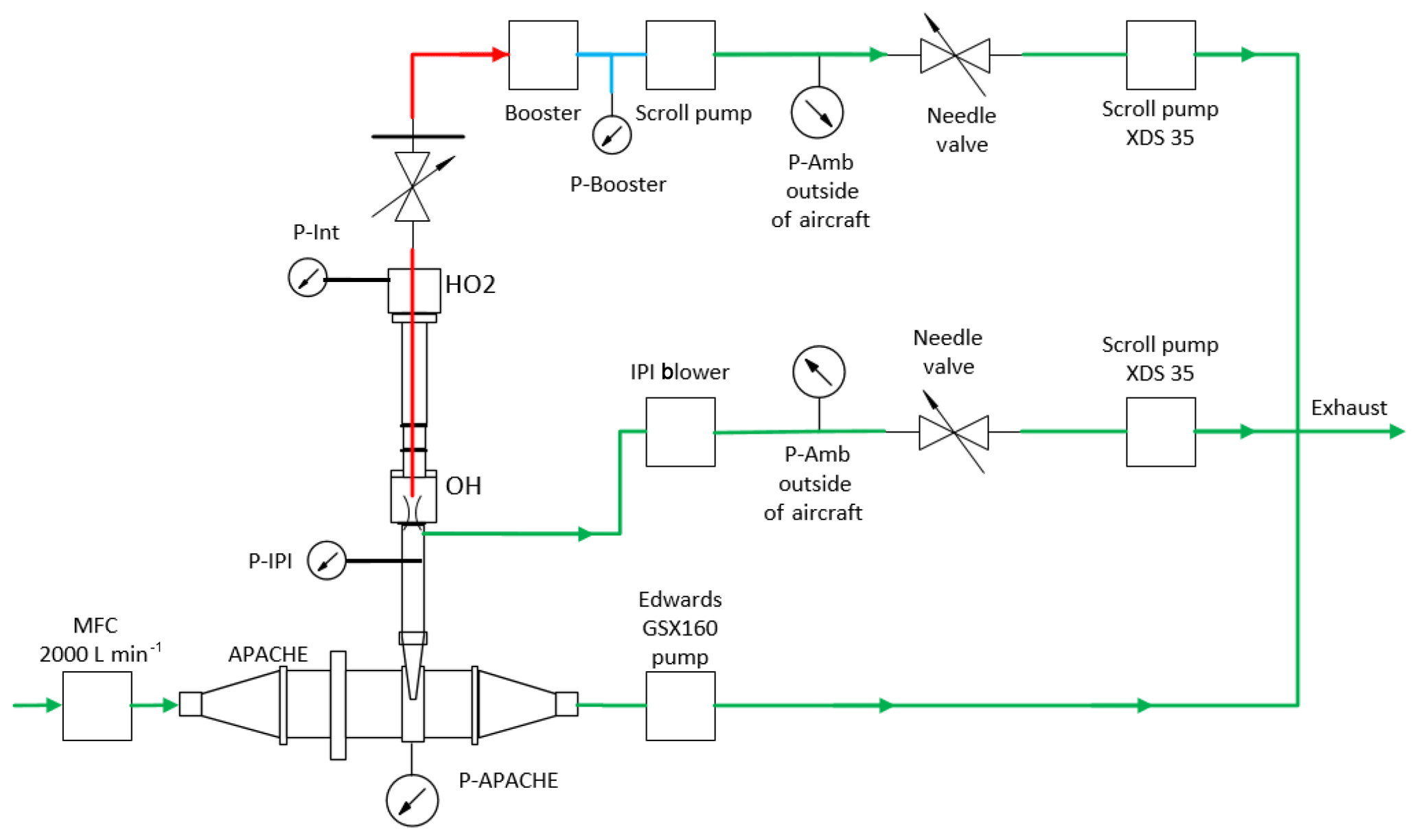
Figure 4 The experimental setup with the additional needle valves, pressure sensors, and XDS35 scroll pumps attached to the exhausts of all pumps and blowers of HORUS to match in-flight pumping efficiencies when calibrating with APACHE. The red lines depict the low-pressure region within HORUS, the blue is the pressure monitoring line between the booster and scroll pump that drive the HORUS sample flow, and the green shows the external gas lines.

To limit the effect of wall loss, HORUS samples air from the core of the APACHE flow system and draws only a fraction of the total airflow as shown in Fig. 5. At 900 hPa the HORUS instrument takes 20 % and at 275 hPa HORUS takes 30 % of the total volume flow entering APACHE. To validate that this proportional volume flow into HORUS does not disturb the flow conditions within APACHE, flow speed profiles were performed using the Prandtl pitot tube installed directly opposite the IPI nozzle, which can be positioned flush against the internal wall up to 60.5 mm into the APACHE cavity, which is 15 mm from the APACHE center. Figure 6 shows the measured flow speed profile (blue data points) when the APACHE pressure was 920 hPa. As the distance between the APACHE wall and the pitot tube inlet increased, no significant change in the flow speed was observed. The largest change observed was between 46.6 and 60.5 mm where the flow speed increased by 0.16 m s⁻¹, which is 22.8 % smaller than the combined uncertainty of these two measurements ±0.21 m s⁻¹ (2σ). Compared to the other four measurement points performed at 920 mbar, the 1.54 m s⁻¹ measured at 60.5 mm is not significantly different. However, when performing the speed profile tests at lower pressures, the pressure difference measured was close to or below the resolution of the differential pressure sensor. Consequently, the flow inside APACHE and the IPI nozzle was simulated using the computational fluid dynamics (CFD) model from COMSOL Multiphysics to gain a better understanding of the flow speed profiles at all pressures. The CFD module in COMSOL uses Reynolds-averaged Navier–Stokes (RANS) models (COMSOL, 2019). The standard k-epsilon turbulence model with incompressible flows was used for this study as it is applicable when investigating flow speeds below 115 m s⁻¹ (COMSOL, 2019). An extra fine gridded mesh of a perforated plate with a high solidity (σ_s=0.96) was implemented in the turbulence model to generate the turbulence and replicate the flows created by the bronze sintered filter (Roach, 1987). The model was constrained with the pressures measured within APACHE and IPI. The volume flow was calculated from the measured mass flow entering APACHE, and temperatures were constrained using the thermistor readings. To gain confidence in the model, the flow speed output data were compared to the available measured flow speed profile (see Fig. 6).

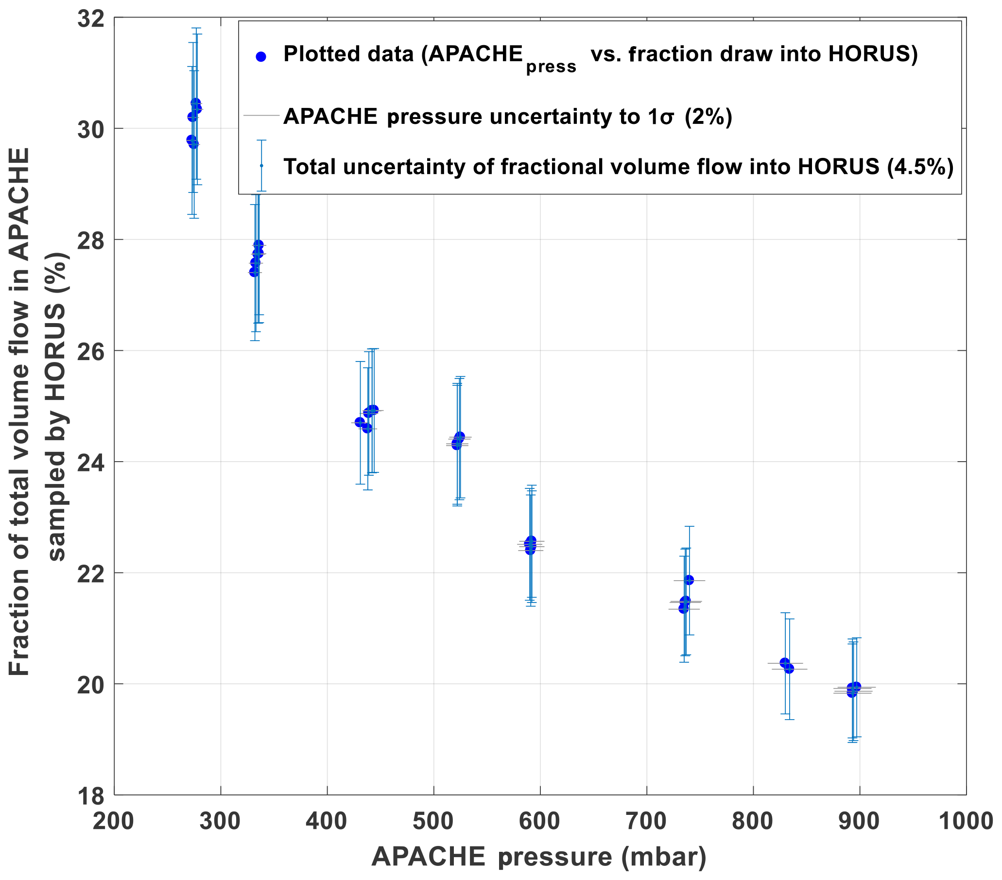
Figure 5 The percentage of the total volume flow entering APACHE, which is sampled by HORUS as a function of pressure within APACHE. All error bars are quoted to 1σ.

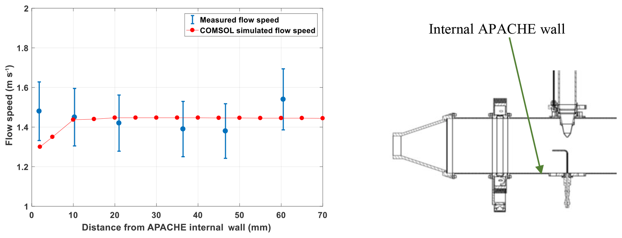
Figure 6 The measured (blue) and COMSOL simulated (red) flow speed profiles within APACHE, at 920 hPa. The x axis is the distance from the internal wall of APACHE. The error bars are quoted to 2σ.

Overall, the modeled flow speed profile did not differ significantly from that measured. The only point where the model significantly disagreed with measurements was at the boundary (<4 mm away from the APACHE wall), where the model predicted a flow speed of 1.3 m s⁻¹, which is 6 % lower than the minimum extent of the measurement uncertainty 1.38 m s⁻¹. This disagreement could also be due to the uncertainty in the parametrization of the boundary conditions in the COMSOL simulations. However, as this is occurring within a region that ultimately does not influence the air entering HORUS (see Sect. 4.1.2), the disagreement between modeled and measured flow speeds at distances less than 4 mm from the APACHE wall is ignored. Figure 7 shows the simulated flow speeds at six discrete pressures within APACHE.

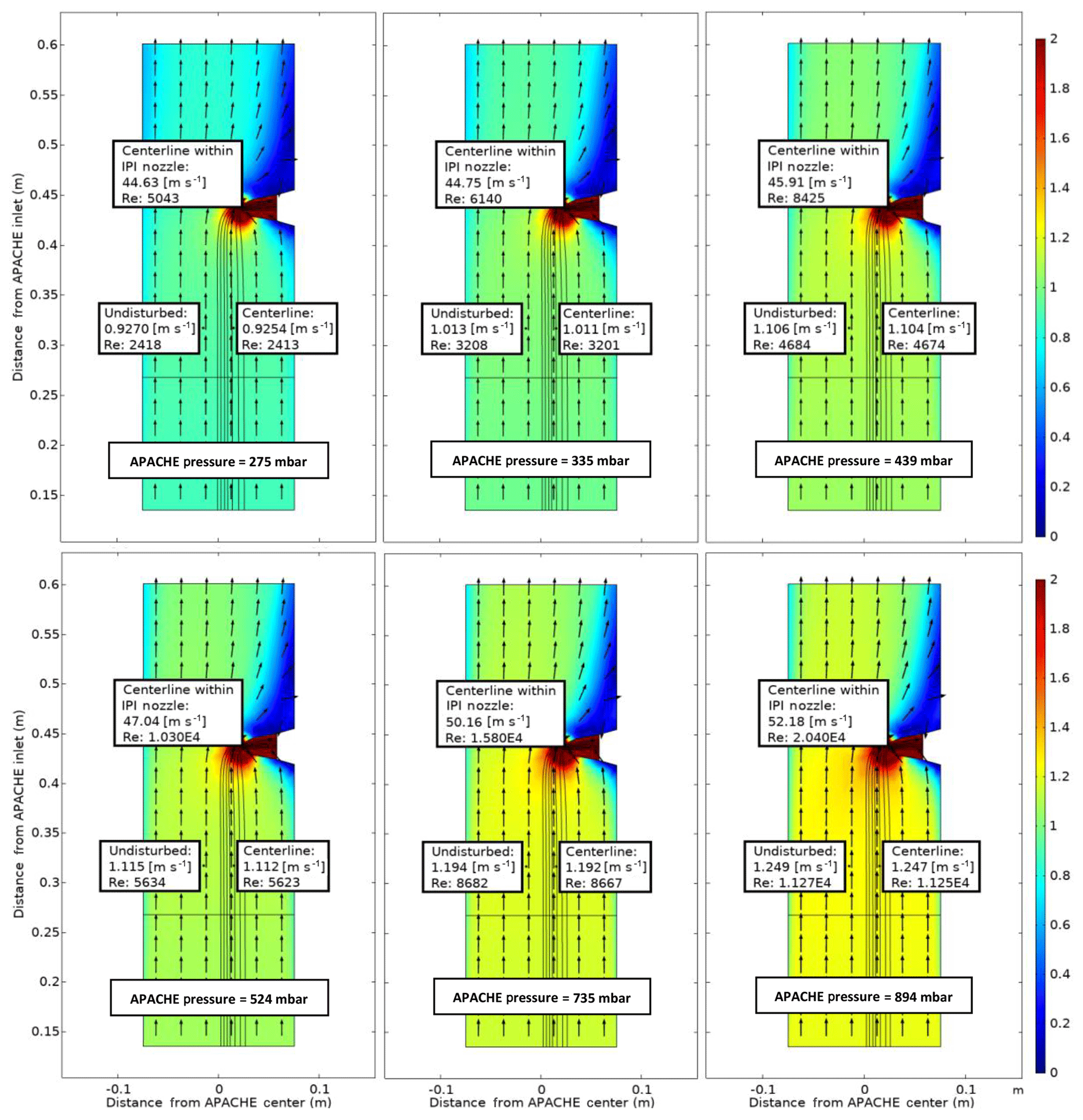
Figure 7 COMSOL Multiphysics output data, simulating the flow speed conditions at six discrete pressures within APACHE ranging from 275 to 894 mbar, between the sintered filter and the first perforated stainless-steel plate. The color represents flow speed in meters per second (m s⁻¹). The black lines are the streamlines created by the HORUS sample flow. The black arrows depict the flow direction. The x axis is the distance from the center of APACHE in meters. The y axis is the distance from the APACHE inlet. The “centerline within the IPI nozzle” labels show the flow conditions in the center of the fully formed flows after the HORUS pinhole, the “undisturbed” labels show the flow conditions outside of the HORUS streamlines, and the “centerline” labels show the flow conditions in the center of the streamlines (i.e., the area of flow influenced by HORUS sampling).

The black lines depict the streamlines of the HORUS sample flow and the color gradient relates to the flow speed. The flow conditions in the center flow within the IPI nozzle, the center of the streamlines, and the undisturbed flow airflow not influenced by the sample flow of the HORUS instrument are indicated. The figure shows the internal APACHE dimensions starting from the sintered filter to the first perforated stainless-steel plate 0.135 and 0.601 m from the APACHE inlet, respectively. From the simulations, the centerline flow speed differs by less than 0.1 % compared to the undisturbed flow, which is also the case at 275 mbar when HORUS is drawing in the highest percentage of the total volume flow entering APACHE. After the sintered filter the high calculated Reynolds numbers (Re>2300) support the statement that a turbulent flow regime is created. Additionally, the measurements in conjunction with simulations show that the small pores of the sintered filter release a uniform distribution of small turbulent elements across the diameter of APACHE, which remain prevalent all the way up to the IPI nozzle.

4.1.2 HO_x losses in APACHE

The modeled OH mixing ratios (pptv) in Fig. 8 show the change in OH content as the air flows along the length of APACHE. Mixing ratios were used as they are independent of the changing density within APACHE. In every simulation, the OH and HO₂ concentrations were initialized at zero, and losses at the walls were fixed to 100 % for both OH and HO₂. The radial photolytic production of OH and HO₂, as calculated using Eqs. (7) and (9), occurred when the air passed the UV ring lamp. For all simulations, the HO_x radical–radical recombination loss reactions (Reactions R6–R8) and the measured molecular diffusion coefficient of OH_Dm in air (Tang et al., 2014) were used:

$${\mathrm{OH}}_{\mathrm{Dm}}=\mathrm{179}(\pm \mathrm{20})\mathrm{Torr}{\mathrm{cm}}^{\mathrm{2}}{\mathrm{s}}^{-\mathrm{1}}\left(\mathrm{239}\pm \mathrm{27}\mathrm{hPa}{\mathrm{cm}}^{\mathrm{2}}{\mathrm{s}}^{-\mathrm{1}}\right).$$

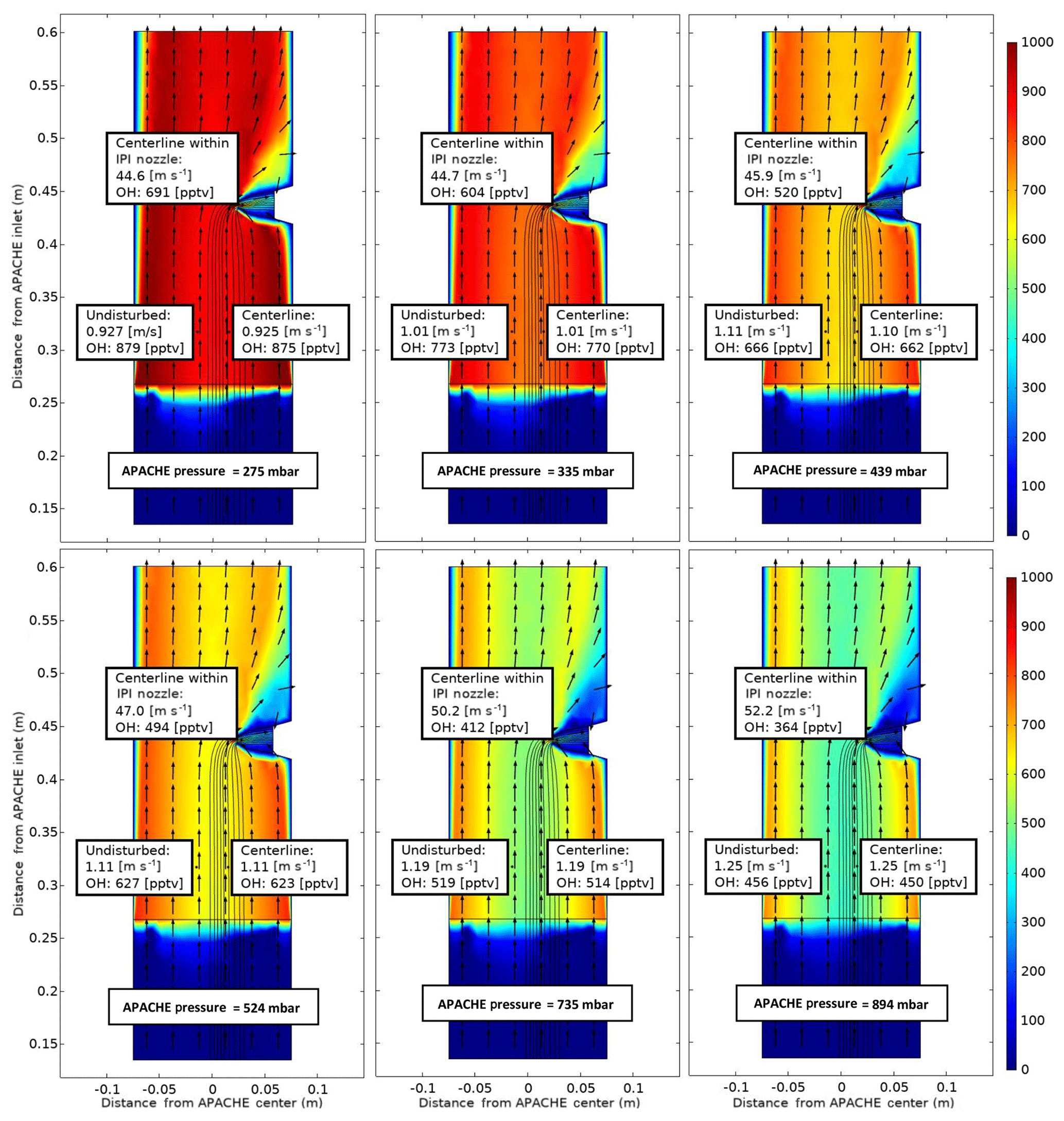
Figure 8 COMSOL Multiphysics output data, simulating OH conditions at six discrete pressures within APACHE ranging from 275 to 894 mbar, between the sintered filter and the first perforated stainless-steel plate. The color gradient is the OH mixing ratio (pptv), with initial OH production occurring at the lamp (0.26 m from APACHE inlet), using Eqs. (7) and (9), with water vapor mixing ratios kept constant at 3.2 mmol mol⁻¹. The black lines are the streamlines created by the HORUS sample flow. The black arrows depict the flow direction. The x axis is the distance from the center of APACHE in meters. The y axis is the distance from the APACHE inlet. The “centerline within IPI nozzle” labels represent the flow and OH concentrations in the center of the fully formed flows after the HORUS pinhole. The “undisturbed” labels show the flow conditions outside of the HORUS streamlines, and the “centerline” labels show the flow conditions in the center of the streamlines (i.e., influenced by HORUS sampling).

In literature, there have been no reports of successfully performed tests that accurately measure HO₂ diffusivity coefficients in air. However, calculations of HO₂ diffusion coefficients using the Lennard-Jones potential model have been performed (Ivanov et al., 2007). Ivanov et al. (2007) performed a series of measurements and Lennard-Jones potential model calculations to quantify the polar analogue diffusion coefficients for OH, HO₂, and O₃ in both air and pure helium. The calculated OH and O₃ diffusion coefficients in air from the Lennard-Jones potential model were in good agreement with the recommended measurement values in Tang et al. (2014) and were well within the given uncertainties. Therefore, to best replicate the diffusivity of HO₂ within the simulations, the following diffusion coefficient of HO₂ in air from the Ivanov et al. (2007) paper was used:

$${\mathrm{HO}}_{\mathrm{2}\mathrm{Dm}}=\mathrm{107.1}\mathrm{Torr}{\mathrm{cm}}^{\mathrm{2}}{\mathrm{s}}^{-\mathrm{1}}\left(\mathrm{142.8}\mathrm{hPa}{\mathrm{cm}}^{\mathrm{2}}{\mathrm{s}}^{-\mathrm{1}}\right).$$

It is clear from Fig. 8 that irrespective of pressure the air masses at the boundary (where wall losses are 100 %) do not have sufficient time to expand into the HORUS sample flow streamlines and influence HO_x content entering HORUS. Lateral exchanges between air at the walls of APACHE and the free air in the center are suppressed due to the preservation of the small turbulence regime between the sintered filter and IPI. Table 2 provides, for six pressures, the evolution of OH along the length of APACHE, within the streamlines created by the HORUS sample flow as depicted in Fig. 8.

Table 2 The evolution of OH within the HORUS sample flow streamlines, along the length of APACHE at all six pressures, within the streamlines created by HORUS sampling as depicted in Fig. 8. The L term represents OH mixing ratios on the left most streamline, C represents OH mixing ratios in the center of the streamlines, and R represents OH mixing ratios on the right most streamline. The centerline within IPI nozzle column shows the OH mixing ratios in the center of the flow in the HORUS inlet. All standard deviations are quoted to 1σ.

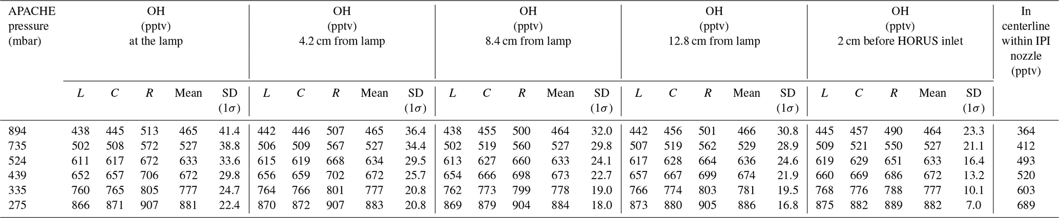
In Table 2, the L term represents OH mixing ratios on the leftmost HORUS sample flow streamline shown in Figs. 7 and 8. C represents OH mixing ratios in the center of the HORUS sample flow streamlines shown in Figs. 7 and 8. R represents OH mixing ratios on the rightmost HORUS sample flow streamline shown in Figs. 7 and 8. The mean mixing ratio at each APACHE pressure does not change significantly and is thus independent of the distance from the lamp. Conversely, the standard deviations of the OH mixing ratios within the HORUS sampling streamlines decrease as the distance from the lamp increases, indicating that the air is homogenizing. However, Fig. 8 and Table 2, with support from available measurements, indicate that the OH-depleted air masses (i.e., air masses that have experienced loss of OH on the APACHE walls) do not expand into and influence the OH content of air that is being sampled by HORUS. The main loss process that influences HO_x entering HORUS is the wall loss occurring at the IPI nozzle itself. According to the COMSOL simulations, around 22.2(±0.8) % (1σ) of OH and HO₂ is lost at the nozzle. This value does not significantly change with pressure, indicating that the HO_x loss at the nozzle is pressure independent. As described in Sect. 2.3, the pressure-independent sensitivity coefficients are a lump sum value containing the pressure-independent wall losses for OH and HO₂. Therefore, the characterized pressure-independent sensitivity coefficients, shown in Sect. 4.3, have the OH and HO₂ losses at the IPI nozzle constrained within them.

4.2 UV conditions

The photolysis lamp is housed in a mount with the side facing into the chamber having an anodized aluminum band with thirty 8 mm apertures installed between the lamp and a quartz wall. The housing was flushed with pure nitrogen to purge any O₂ present before the lamp was turned on. The nitrogen flushing was kept on continuously thereafter. After approximately 1 h, the lamp reached stable operation conditions; i.e., the relative flux emitted by the lamp as measured by a photometer (seen in Fig. 1b at the UVL (ultraviolet lamp) on the underside of the APACHE chamber) was constant. The flux (F_β) entering APACHE is not the same as the flux experienced by the molecules sampled by HORUS (F). Factors influencing the ratio between F_β and F are as follows: (i) absorption of light by O₂, which is particularly important as O₂ has a strong absorption band at 184.9 nm and the O₂ density changes in APACHE when calibrating at the different pressures; (ii) the variable radial flux, which is dependent on the geometric setup of the ring lamp and on the location within the irradiation cross section where the molecule is passing. These factors were resolved through the combination of two actinometrical cross-check methods. The advantage of actinometrical methods is that the flux calculated is derived directly from the actual flux that is experienced by the molecules themselves as they pass through the APACHE chamber.

The first actinometrical method (A) used the HORUS instrument as a transfer standard to relate the flux of a precalibrated Pen-Ray lamp used on the ground-based calibration device to F_β entering APACHE. This entailed first calibrating the HORUS instrument using a precharacterized ground-based calibration device (Martinez et al., 2010). The precalibrated Pen-Ray lamp flux (ϕ₀) is calculated from the measured NO concentrations that are produced by irradiating a known mixture of N₂O in a carrier gas:

$$\begin{array}{}\text{(8)}& {\mathit{\varphi }}_{\mathrm{0}}={\displaystyle \frac{\left(k_{\mathrm{a}}\left[{\mathrm{N}}_{\mathrm{2}}\right]\left[M\right]+k_{\mathrm{b}}\left[{\mathrm{N}}_{\mathrm{2}}\right]+k_{\mathrm{c}}\left[{\mathrm{N}}_{\mathrm{2}}\mathrm{O}\right]+k_{\mathrm{d}}\left[{\mathrm{N}}_{\mathrm{2}}\mathrm{O}\right]\left[\mathrm{NO}\right]\right)}{\mathrm{2}{k}_{\mathrm{d}}{\left[{\mathrm{N}}_{\mathrm{2}}\mathrm{O}\right]}^{\mathrm{2}}{\mathit{\sigma }}_{{\mathrm{N}}_{\mathrm{2}}\mathrm{O}}{f}_{{\mathrm{N}}_{\mathrm{2}}\mathrm{O}}}},\end{array}$$

where ${\mathit{\sigma }}_{{\mathrm{N}}_{\mathrm{2}}\mathrm{O}}$ is the absorption cross section of N₂O at 184.9 nm and $f_{{\mathrm{N}}_{\mathrm{2}}\mathrm{O}}$ is the correction factor that accounts for the flux reduction via absorption by N₂O. A TEI NO monitor measures the NO concentration. For more details on how the ground calibration device is characterized using the photolysis of N₂O in conjunction with a TEI NO monitor, see Martinez et al. (2010). Since the precharacterized ground-based calibration device is designed to supply only 50 sL min⁻¹, and the sensitivity of the airborne HORUS instrument is optimized for high-altitude flying, the critical orifice diameter in HORUS was changed from the airborne configuration of 1.4 to a 0.8 mm on-ground^* configuration. Additionally, the IPI system was switched to passive (i.e., the exhaust line from IPI to the IPI blower was capped). This was to adapt HORUS to a mass flow that the ground-based calibration device is able to provide and reduces the internal pressure within HORUS (from 18 to 3.5 mbar) to optimize the sensitivity towards OH at ambient ground level pressures (∼1000 mbar). The asterisk discerns terms that were quantified when the smaller 0.8 mm critical orifice was used. The calculated instrument on-ground^* sensitivity was then used to translate OH and HO₂ concentrations produced by the uv-technik Hg ring lamp into a value for F_β. Take note that for the direct calibrations of the airborne HORUS system using the characterized APACHE system, discussed in Sect. 4.3, the same initial 1.4 mm diameter critical orifice as used during the airborne campaign was installed. The HORUS on-ground^* sensitivities at 1010 mbar for OH and HO₂ are 13.7(±1.9) and 17.9(±2.5) cts s⁻¹ pptv⁻¹ mW⁻¹ respectively, with the uncertainties quoted to 1σ. This sensitivity was then used to calculate the OH and HO₂ concentrations at the instrument nozzle with the APACHE system installed and operating at 1010 mbar. To ensure sufficient flow stability during calibration at this high pressure, the Edwards GSX160 scroll pump was disengaged. Additionally, the water mixing ratios were kept constant (∼3.1 mmol mol⁻¹) and oxygen levels were varied by adding different pure N₂ and synthetic air mixtures, via MFCs. The OH and HO₂ concentrations at the IPI nozzle were 1.41(±0.01) and $\mathrm{1.31}(\pm \mathrm{0.01})\times {\mathrm{10}}^{\mathrm{10}}$ molecules cm⁻³ respectively when using a water vapor mixing ratio of 3.1 mmol mol⁻¹ in synthetic air injected into APACHE. The uncertainties are quoted as measurement variability at 1σ. Using these values, the OH and HO₂ concentrations at the lamp were back calculated accounting for radical–radical loss Reactions (R6–R8) and HO_x reactions with O₃ (Reactions R9–R10) using rate constants taken from Burkholder et al. (2015) with temperature (T) in Kelvin.

$$\begin{array}{}\text{(R6)}& {\displaystyle }& {\displaystyle }\mathrm{OH}+\mathrm{OH}\to {\mathrm{H}}_{\mathrm{2}}\mathrm{O}+\mathrm{O}{(}^{\mathrm{3}}\mathrm{P})k=\mathrm{1.8}\times {\mathrm{10}}^{-\mathrm{12}}\cdot {\exp }^{\left[\frac{\mathrm{1}}{T}\right]}\text{(R7)}& {\displaystyle }& {\displaystyle }{\mathrm{HO}}_{\mathrm{2}}+{\mathrm{HO}}_{\mathrm{2}}\to {\mathrm{H}}_{\mathrm{2}}{\mathrm{O}}_{\mathrm{2}}+{\mathrm{O}}_{\mathrm{2}}k=\mathrm{3.0}\times {\mathrm{10}}^{-\mathrm{13}}\cdot {\exp }^{\left[\frac{\mathrm{460}}{T}\right]}\text{(R8)}& {\displaystyle }& {\displaystyle }\mathrm{OH}+{\mathrm{HO}}_{\mathrm{2}}\to {\mathrm{H}}_{\mathrm{2}}\mathrm{O}+{\mathrm{O}}_{\mathrm{2}}k=\mathrm{4.8}\times {\mathrm{10}}^{-\mathrm{11}}\cdot {\exp }^{\left[\frac{\mathrm{250}}{T}\right]}\text{(R9)}& {\displaystyle }& {\displaystyle }{\mathrm{HO}}_{\mathrm{2}}+{\mathrm{O}}_{\mathrm{3}}\to \mathrm{OH}+\mathrm{2}{\mathrm{O}}_{\mathrm{2}}k=\mathrm{1.0}\times {\mathrm{10}}^{-\mathrm{14}}\cdot {\exp }^{\left[\frac{-\mathrm{490}}{T}\right]}\text{(R10)}& {\displaystyle }& {\displaystyle }\mathrm{OH}+{\mathrm{O}}_{\mathrm{3}}\to {\mathrm{HO}}_{\mathrm{2}}+{\mathrm{O}}_{\mathrm{2}}k=\mathrm{1.7}\times {\mathrm{10}}^{-\mathrm{12}}\cdot {\exp }^{\left[\frac{-\mathrm{940}}{T}\right]}\end{array}$$

In APACHE when the Edwards GSX160 scroll pump was disengaged, the transit time between the UV radiation zone and the IPI nozzle was 0.18 s, resulting in chemical losses of 30 % to 33 % for OH and 27 % to 30 % HO₂, depending on oxygen concentration. Accounting for these chemical losses yields OH concentrations of $\mathrm{2.0}(\pm \mathrm{0.02})\times {\mathrm{10}}^{\mathrm{10}}$ molecules cm⁻³ and HO₂ concentrations of $\mathrm{1.9}(\pm \mathrm{0.02})\times {\mathrm{10}}^{\mathrm{10}}$ molecules cm⁻³ at the lamp, at 1010 mbar. The photon flux (F) experienced by the air sampled by HORUS, quantified using the OH and HO₂ concentrations stated above, ranged from 3.8×10¹⁴ to 6.7×10¹⁴ photons cm⁻² s⁻¹ depending on oxygen concentrations and considering the chemical losses. As described before, Eq. (7) shows how the production of OH at the lamp is calculated:

$$\begin{array}{}\text{(9)}& \left[\mathrm{OH}\right]=\left[{\mathrm{H}}_{\mathrm{2}}\mathrm{O}\right]\cdot {\mathit{\sigma }}_{{\mathrm{H}}_{\mathrm{2}}\mathrm{O}}\cdot F_{\mathrm{184.9}\mathrm{nm}}\cdot {\mathit{\varphi }}_{{\mathrm{H}}_{\mathrm{2}}\mathrm{O}}\cdot t.\end{array}$$

F_184.9 nm is the actinic flux encountered by the water molecules as they pass across the photolysis region, which is dependent on the attenuation of the flux (F_β) entering APACHE due to water vapor and O₂ molecules. Whereas the absorption coefficient of water vapor is constant across the linewidth of the 184.9 nm Hg emission line, the effective absorption cross section of molecular oxygen (${\mathit{\sigma }}_{{\mathrm{O}}_{\mathrm{2}}}$) changes significantly at 184.9 nm within the linewidth of the Hg lamp (Creasey et al., 2000). Therefore, ${\mathit{\sigma }}_{{\mathrm{O}}_{\mathrm{2}}}$ affecting the APACHE calibrations is dependent on O₂ concentration and the ring lamp temperature and current. Since the operating temperature of the uv-technik Hg lamp and the current applied (0.8 A) was kept constant during the actinometrical experiments and during the APACHE calibrations, any effect on ${\mathit{\sigma }}_{{\mathrm{O}}_{\mathrm{2}}}$ regarding the ring lamp linewidth does not need to be investigated further in this study. The relationship of F_184.9 nm to F_β can be derived using Beer–Lambert principles:

$$\begin{array}{}\text{(10)}& F_{\mathrm{184.9}\mathrm{nm}}=F_{\mathit{\beta }}\cdot e^{-}\left({\mathit{\gamma }}_{{\mathrm{H}}_{\mathrm{2}}\mathrm{O}}\left[{\mathrm{H}}_{\mathrm{2}}\mathrm{O}\right]+{\mathit{\gamma }}_{{\mathrm{O}}_{\mathrm{2}}}\left[{\mathrm{O}}_{\mathrm{2}}\right]\right),\end{array}$$

where F_β is the flux intensity entering APACHE from the ring lamp, with

$$\begin{array}{}\text{(11)}& {\mathit{\gamma }}_{{\mathrm{O}}_{\mathrm{2}}}=R_{\mathit{\beta }}\cdot \mathit{\omega }\cdot {\mathit{\sigma }}_{{\mathrm{O}}_{\mathrm{2}}},\end{array}$$

where R_β is the radial distance of the sampled air parcel to the ring lamp of APACHE; ω is a correction factor replicating the integrated product of the absorption cross section and the ring lamp's emission line as modified by the effect of the absorption of O₂ present in between the lamp; and the flight path of the sampled air, normalized by ${\mathit{\sigma }}_{{\mathrm{O}}_{\mathrm{2}}}$, is the effective cross section of O₂. When combining Eqs. (7) and (9) the OH concentration produced at the lamp is quantified as

$$\begin{array}{}\text{(12)}& \begin{array}{rl}\left[\mathrm{OH}\right]& =\left[{\mathrm{H}}_{\mathrm{2}}\mathrm{O}\right]\cdot {\mathit{\sigma }}_{{\mathrm{H}}_{\mathrm{2}}\mathrm{O}}\cdot {\mathit{\varphi }}_{{\mathrm{H}}_{\mathrm{2}}\mathrm{O}}\cdot t\cdot F_{\mathit{\beta }}\\ & \cdot e^{-}\left({\mathit{\gamma }}_{{\mathrm{H}}_{\mathrm{2}}\mathrm{O}}\left[{\mathrm{H}}_{\mathrm{2}}\mathrm{O}\right]+{\mathit{\gamma }}_{{\mathrm{O}}_{\mathrm{2}}}\left[{\mathrm{O}}_{\mathrm{2}}\right]\right)\end{array}.\end{array}$$

Equation (11) can be rearranged to

$$\begin{array}{}\text{(13)}& \begin{array}{rl}\ln \left[{\displaystyle \frac{\left[\mathrm{OH}\right]}{\left[{\mathrm{H}}_{\mathrm{2}}\mathrm{O}\right]}}\right]& =\ln \left(F_{\mathit{\beta }}\cdot t\cdot {\mathit{\varphi }}_{{\mathrm{H}}_{\mathrm{2}}\mathrm{O}}\cdot {\mathit{\sigma }}_{{\mathrm{H}}_{\mathrm{2}}\mathrm{O}}\right)\\ & +\left(-{\mathit{\gamma }}_{{\mathrm{H}}_{\mathrm{2}}\mathrm{O}}\cdot \left[{\mathrm{H}}_{\mathrm{2}}\mathrm{O}\right]-{\mathit{\gamma }}_{{\mathrm{O}}_{\mathrm{2}}}\cdot \left[{\mathrm{O}}_{\mathrm{2}}\right]\right)\end{array}.\end{array}$$

Figure 9 shows the measured production of OH (left side of Eq. 12) plotted against oxygen concentration. Given that the other terms within Eq. (12) are constant with changing oxygen levels, the plotted gradient of the linear regression in Fig. 9 yields γ_O2 as a function of oxygen concentration being $\mathrm{1.2}\times {\mathrm{10}}^{-\mathrm{19}}(\pm \mathrm{0.05}\times {\mathrm{10}}^{-\mathrm{19}})$ cm³ per molecule.

Figure 9 Plot showing the result of Eq. (11) as a function of oxygen concentration.

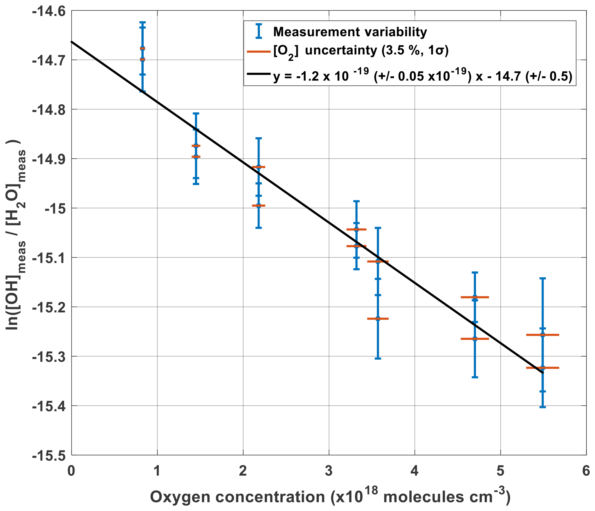
Given that the y intercept of the linear regression, −14.66, is equal to the natural logarithm of ($F_{\mathit{\beta }}t{\mathit{\varphi }}_{{\mathrm{H}}_{\mathrm{2}}\mathrm{O}}$) minus $\left({\mathit{\gamma }}_{{\mathrm{H}}_{\mathrm{2}}\mathrm{O}}\right[{\mathrm{H}}_{\mathrm{2}}\mathrm{O}\left]\right)$, the flux entering APACHE F_β can be characterized:

$$\begin{array}{}\text{(14)}& \begin{array}{rl}{F}_{\mathit{\beta }}& =\left({\displaystyle \frac{e^{-\mathrm{14.66}}}{t\cdot {\mathit{\varphi }}_{{\mathrm{H}}_{\mathrm{2}}\mathrm{O}}}}\right)-\left({\mathit{\gamma }}_{{\mathrm{H}}_{\mathrm{2}}\mathrm{O}}\cdot \left[{\mathrm{H}}_{\mathrm{2}}\mathrm{O}\right]\right)\\ & =\mathrm{6.9}\times {\mathrm{10}}^{\mathrm{14}}(\pm \mathrm{1.1}\times {\mathrm{10}}^{\mathrm{14}})\mathrm{photons}{\mathrm{cm}}^{-\mathrm{2}}{\mathrm{s}}^{-\mathrm{1}}\end{array}.\end{array}$$

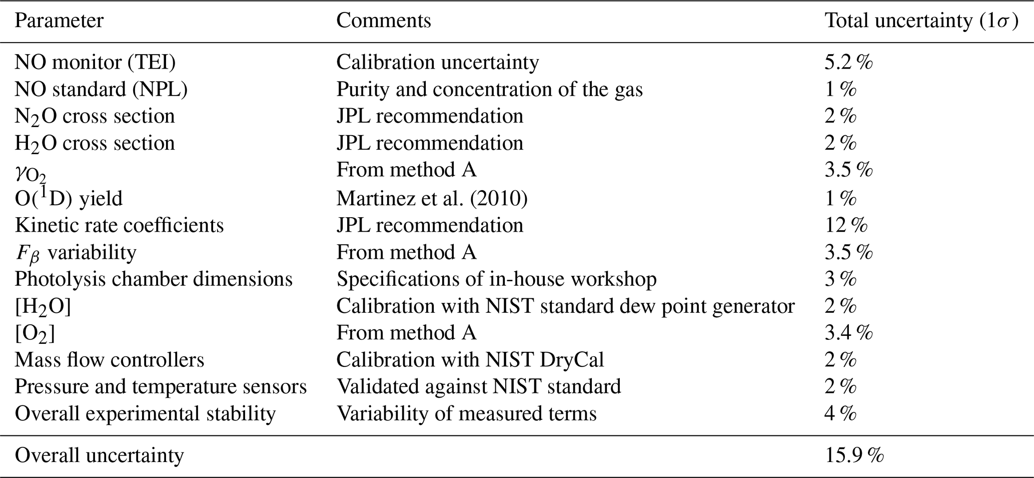
The accuracy in F_β from method A is 15.9 % (1σ). Table 3 shows the parameters and their uncertainties contributing to the F_β characterized in method A.

Table 3 Parameters and uncertainties used in method A, using HORUS as a transfer standard. Overall uncertainty is the sum of the quadrature of the individual uncertainties. O(¹D) yield is taken from Martinez et al. (2010).

The second actinometrical method (B) involved using an ANSYCO O3 41 M ozone monitor to measure the ozone mixing ratio profile between the IPI nozzle and the wall surface of APACHE, at ground pressure (1021 mbar). This method utilizes O₂ photolysis at 184.9 nm, which produces two O(³P) atoms capable of reacting with a further two O₂ molecules to produce O₃.

$$\begin{array}{}\text{(R11)}& {\displaystyle }& {\displaystyle }{\mathrm{O}}_{\mathrm{2}}+hv\to \mathrm{O}{(}^{\mathrm{3}}\mathrm{P})+\mathrm{O}{(}^{\mathrm{3}}\mathrm{P})\text{(R12)}& {\displaystyle }& {\displaystyle }{\mathrm{O}}_{\mathrm{2}}+\mathrm{O}{(}^{\mathrm{3}}\mathrm{P})+M\to {\mathrm{O}}_{\mathrm{3}}+M\end{array}$$

The value of $\mathrm{1.2}\times {\mathrm{10}}^{-\mathrm{19}}$ cm³ per molecule for ${\mathit{\gamma }}_{{\mathrm{O}}_{\mathrm{2}}}$ found in the previous method was used to calculate the actinic flux entering APACHE:

$$\begin{array}{}\text{(15)}& F_{\mathit{\beta }}={\displaystyle \frac{\left[{\mathrm{O}}_{\mathrm{3}}\right]}{\left[{\mathrm{O}}_{\mathrm{2}}\right]\cdot {\mathit{\gamma }}_{{\mathrm{O}}_{\mathrm{2}}}\cdot {\mathit{\varphi }}_{{\mathrm{O}}_{\mathrm{2}}}\cdot t\cdot e^{-\left({\mathit{\gamma }}_{{\mathrm{O}}_{\mathrm{2}}}\left[{\mathrm{O}}_{\mathrm{2}}\right]\right)}}}.\end{array}$$

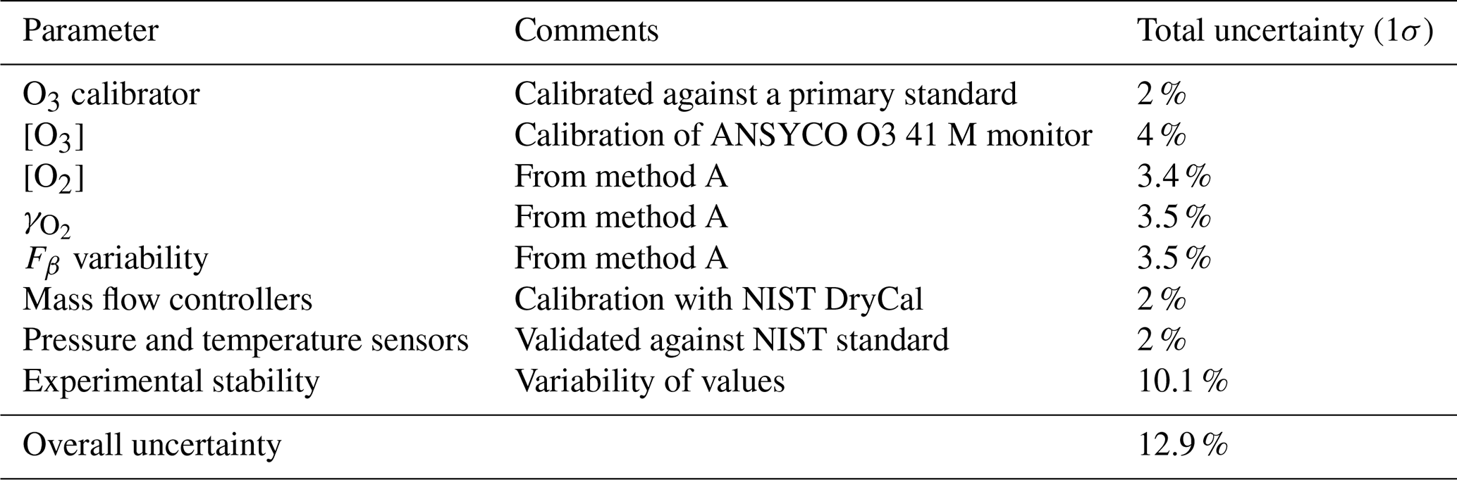
${\mathrm{\Phi }}_{{\mathrm{O}}_{\mathrm{2}}}$ is the quantum yield of O₂ at 184.9 nm, which has been determined to be 1 between 242 and 175 nm (Atkinson et al., 2004). As in method A, the ozone produced at the lamp is quantified by back calculating from the ozone measured at the ANSYCO O3 41 M inlet position. Inside APACHE, typical ozone concentrations ranged from 1.26×10¹² to 2.05×10¹² molecules cm⁻³ depending on the oxygen concentration. From this approach, the calculated F_β is $\mathrm{6.11}\times {\mathrm{10}}^{\mathrm{14}}(\pm \mathrm{0.8}\times {\mathrm{10}}^{\mathrm{14}})$ photons cm⁻² s⁻¹ with a total uncertainty of 12.9 % (1σ). The final value taken for F_β is the average of the two experiments, weighted by their uncertainties:

• actinic flux ($F_{\mathit{\beta }})=\mathrm{6.37}\times {\mathrm{10}}^{\mathrm{14}}(\pm \mathrm{1.3}\times {\mathrm{10}}^{\mathrm{14}})$ photons cm⁻² s⁻¹

• accuracy in F_β=20.5 % (1σ)

• agreement for F_β between method A and B, zeta score =0.59.

Table 4 shows the parameters and their uncertainties which contribute to the F_β characterized in method B.

Table 4 Parameters and uncertainties involved in method B, using the ANSYCO O3 41 M monitor. The total uncertainty is the sum of the quadrature of the individual uncertainties.

4.3 Evaluation of instrumental sensitivity

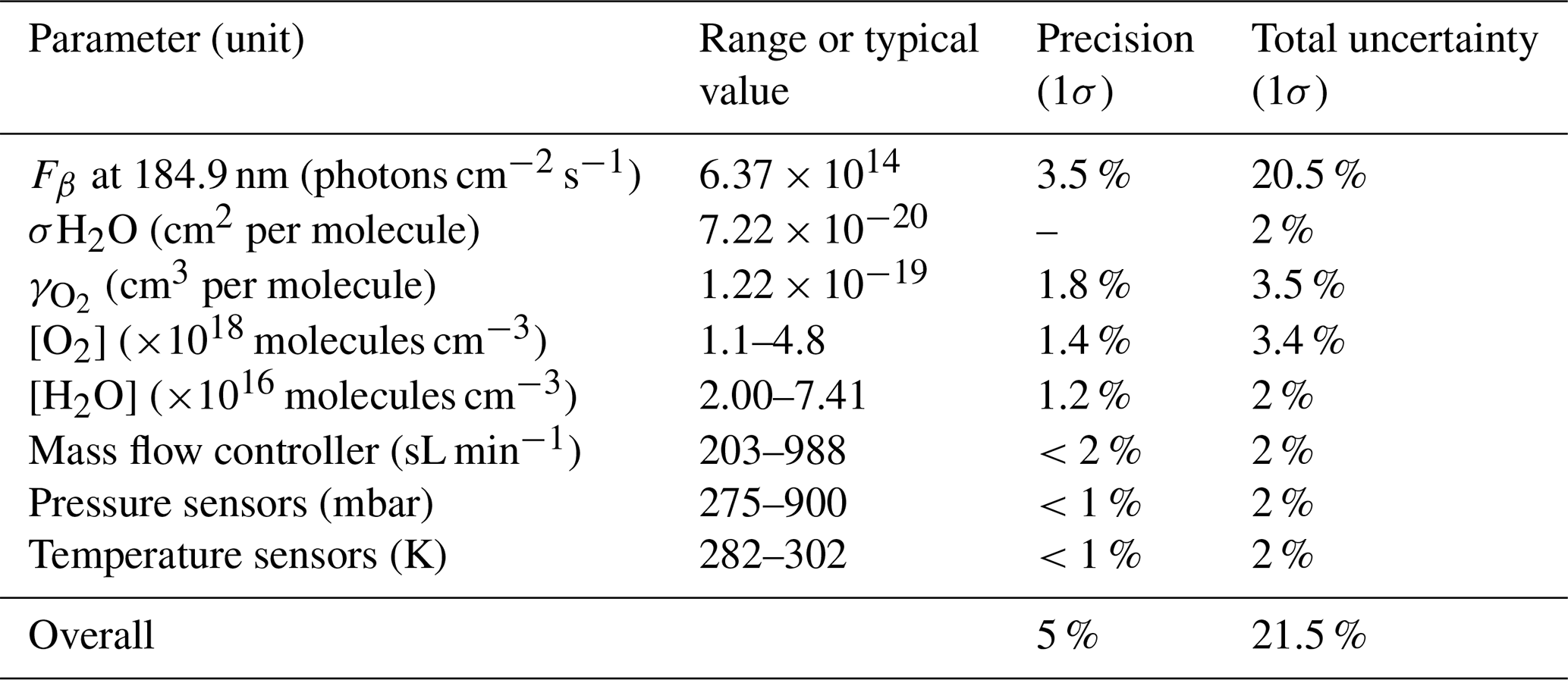
Figure 10 shows the sensitivity curve of HORUS; the quenching effect; the linear fits used to quantify the pressure-independent sensitivity coefficients; and relative HO_x transmission values for OH, OH in the second axis, and HO₂ plotted as a function of the HORUS internal density. The red smoothed line in Fig. 10a represents the calculated sensitivity curve for each measurement using Eq. (4) and the characterized variables therein. Given that this calculated sensitivity curve for each measurement agrees to within 2σ of the uncertainties in measured calibration curves, we are confident that each of the terms described in Eq. (4) has been sufficiently resolved. Table 5 shows the ranges, precision, and uncertainties of measured or calculated variables affecting OH and HO₂ concentrations formed in APACHE.

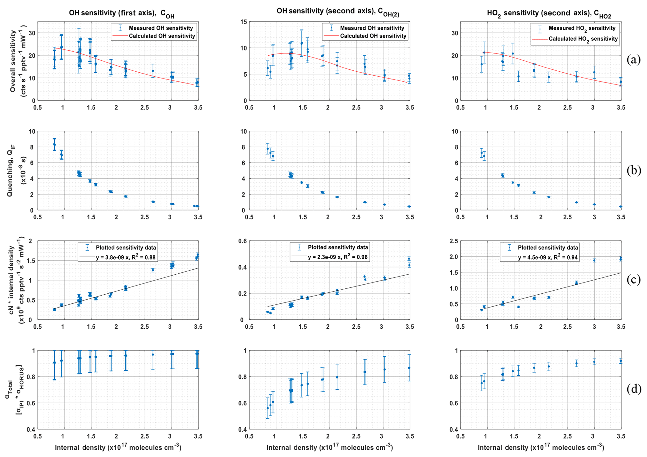
Figure 10 The determination of the pressure-based sensitivity of OH in both axes and HO₂ for HORUS. The data shown are 1 h averages for the tested pressures, all plotted with the internal density on the x axis. Row (a) is the measured (blue data points) HORUS sensitivity curve and calculated (red line) sensitivity curve. Row (b) is internal quenching by N₂, O2, and water vapor. Row (c) is internal density and the pressure-independent sensitivity coefficient (cN; c0 for the OH first axis, c1 for OH second axis, and c2 for HO₂). Row (d) is the total OH and HO₂ transmissions, all plotted against internal density. The error bars represent measurement variability (1σ) for rows (b, c). In rows (a, d), the error bars represent the total uncertainty (1σ).

Table 5 Parameters within APACHE, their ranges, and uncertainties, contributing to the uncertainty in the three measurement sensitivities within HORUS.

The pressure-independent sensitivity coefficients (cN) for OH in the first axis (c0), OH in the second axis (c1), and HO₂ in the second axis (c2) are calculated by rearranging Eq. (4) to

$$\begin{array}{}\text{(16)}& {\displaystyle }\begin{array}{rl}& \text{c0}\cdot {\mathit{\rho }}_{\mathrm{Int}}\left(P,T\right)\\ & ={\displaystyle \frac{C_{\mathrm{OH}}\left(P,T\right)}{Q_{\mathrm{IF}}\left(P,T\right)\cdot b_{\mathrm{c}}\left(T\right)\cdot \left[{\mathit{\alpha }}_{\mathrm{IPI}\mathrm{OH}}\left(P,T\right)\cdot {\mathit{\alpha }}_{\mathrm{HORUS}\mathrm{OH}}\left(P,T\right)\right]}}\end{array},\text{(17)}& {\displaystyle }\begin{array}{rl}& \text{c1}\cdot {\mathit{\rho }}_{\mathrm{Int}}\left(P,T\right)\\ & ={\displaystyle \frac{C_{\mathrm{OH}\left(\mathrm{2}\right)}\left(P,T\right)}{Q_{\mathrm{IF}\left(\mathrm{2}\right)}\left(P,T\right)\cdot b_{\mathrm{c}}\left(\mathrm{T}\right)\cdot \left[{\mathit{\alpha }}_{\mathrm{IPI}\mathrm{OH}}\left(P,T\right)\cdot {\mathit{\alpha }}_{\mathrm{HORUS}\mathrm{OH}\left(\mathrm{2}\right)}\left(P,T\right)\right]}}\end{array},\text{(18)}& {\displaystyle }\begin{array}{rl}& \text{c2}\cdot {\mathit{\rho }}_{\mathrm{Int}}\left(P,T\right)\\ & ={\displaystyle \frac{C_{{\mathrm{HO}}_{\mathrm{2}}}\left(P,T\right)}{Q_{\mathrm{IF}\left(\mathrm{2}\right)}\left(P,T\right)\cdot b_{\mathrm{c}}\left(T\right)\cdot \left[{\mathit{\alpha }}_{\mathrm{IPI}{\mathrm{HO}}_{\mathrm{2}}}\left(P,T\right)\cdot {\mathit{\alpha }}_{\mathrm{HORUS}{\mathrm{HO}}_{\mathrm{2}}}\left(P,T\right)\right]}}\end{array}.\end{array}$$

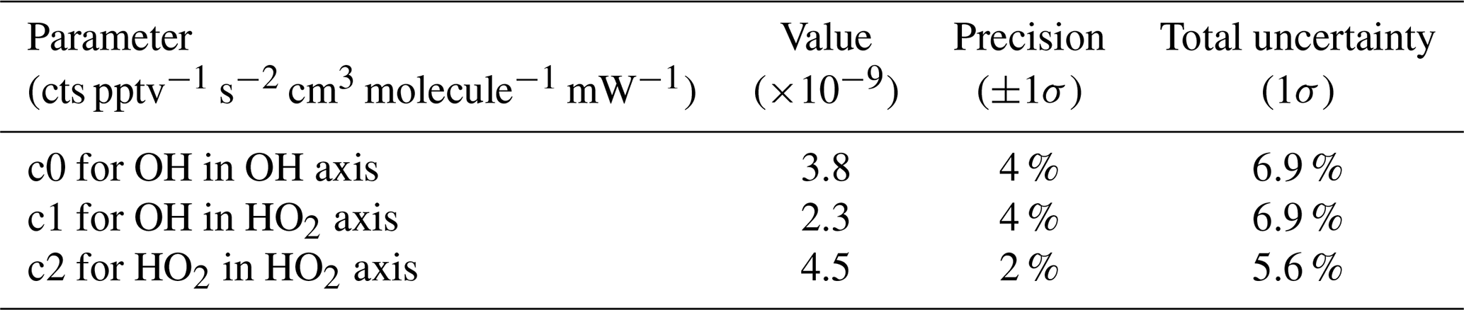
The products of Eq. (15) to (17) are plotted against internal density in Fig. 10c, where the slopes of the linear regressions are the pressure-independent sensitivity coefficients. Note that in Eqs. (16) and (17) the two bracketed terms are in relation to the OH measurement at the second axis. Table 6 shows the values, precision, and uncertainty in the quantified pressure-independent sensitivity coefficients.

Table 6 Pressure-independent sensitivities and their overall uncertainty from calibrations with APACHE.

In Fig. 10c the quenching (Q_IF) is plotted against internal density. Q_IF is calculated using the same approach as described in Faloona et al. (2004) and Martinez et al. (2010):

$$\begin{array}{}\text{(19)}& Q_{\mathrm{IF}}\left(P\right)={\displaystyle \frac{\mathrm{1}}{\mathrm{\Gamma }}}\left(e^{-\mathrm{\Gamma }{g}_{\mathrm{1}}}-e^{-\mathrm{\Gamma }{g}_{\mathrm{2}}}\right),\end{array}$$

where Γ is the excited state decay frequency (Hz), consisting of the natural decay frequency, and decay due to collisional quenching that is dependent on pressure, temperature, and water vapor mixing ratio. g₁ and g₂ are the detector gate opening and closing times after the initial excitation laser pulse, which are set to 104 and 600 ns respectively.

As described in Sect. 2.3, the pressure-independent sensitivity coefficients are lump sum variables containing pressure-independent HO_x wall loss. The pressure-dependent HO_x transmission through the HORUS instrument is quantified and described below. In flight, IPI operates across the pressure range of 180 to 1010 mbar. However, within HORUS, post critical orifice, at detection axes where HO_x is measured the pressure ranges from 3.1 to 18.4 mbar. Therefore, the transmission through IPI (α_IPI) and through HORUS (α_HORUS) must be quantified separately using the corresponding measured pressures and transit times, before being combined as the total transmission (${\mathit{\alpha }}_{\mathrm{IPI}}\cdot {\mathit{\alpha }}_{\mathrm{HORUS}}={\mathit{\alpha }}_{\mathrm{Total}}$). To calculate the transmission of HO_x within IPI, the following was used:

$$\begin{array}{}\text{(20)}& {\displaystyle }& {\displaystyle }{\mathit{\alpha }}_{\mathrm{IPI}\mathrm{OH}}=\mathrm{1}-⌈{\displaystyle \frac{{\mathrm{OH}}_{\mathrm{DM}}\left(P\right)\cdot t_{\mathrm{r}\mathrm{IPI}}(P,T)\cdot \mathit{\pi }}{{\text{IPI}}_{\mathrm{A}}\cdot P_{\mathrm{IPI}}}}⌉,\text{(21)}& {\displaystyle }& {\displaystyle }{\mathit{\alpha }}_{\mathrm{IPI}{\mathrm{HO}}_{\mathrm{2}}}=\mathrm{1}-⌈{\displaystyle \frac{{\mathrm{HO}}_{\mathrm{2}\mathrm{DM}}\left(P\right)\cdot t_{\mathrm{r}\mathrm{IPI}}\left(P,T\right)\cdot \mathit{\pi }}{{\text{IPI}}_{\mathrm{A}}\cdot P_{\mathrm{IPI}}}}⌉,\end{array}$$

where t_r IPI is the transit time within IPI, i.e., the time it takes for air to flow from the IPI nozzle to the critical orifice of HORUS. IPI_A is the internal cross-sectional area of IPI and P_IPI is the measured pressure within IPI. The OH_DM and HO_2 DM terms are the OH and HO₂ diffusion coefficients as described in Sect. 4.1.2. α_IPI OH is the transmission of OH through IPI, and ${\mathit{\alpha }}_{\mathrm{IPI}{\mathrm{HO}}_{\mathrm{2}}}$ is the transmission of HO₂ through IPI. By applying Eqs. (19) and (20), α_IPI OH and ${\mathit{\alpha }}_{\mathrm{IPI}{\mathrm{HO}}_{\mathrm{2}}}$ ranged from 0.97 to 0.99 and 0.99 to 0.997 respectively across the pressure range within IPI of 198–808 mbar and IPI transit times of 90–120 ms. However, to calculate α_Total, the OH and HO₂ transmission post critical orifice, α_HORUS OH and ${\mathit{\alpha }}_{\mathrm{HORUS}{\mathrm{HO}}_{\mathrm{2}}}$, must be resolved. α_HORUS regarding OH and HO₂ can be calculated by adapting Eqs. (19) and (20) to the internal HORUS conditions producing:

$$\begin{array}{}\text{(22)}& {\displaystyle }& {\displaystyle }{\mathit{\alpha }}_{\mathrm{HORUS}\mathrm{OH}}=\mathrm{1}-⌈{\displaystyle \frac{{\mathrm{OH}}_{\mathrm{DM}}\left(P\right)\cdot t_{\mathrm{r}\mathrm{1}}\left(P,T\right)\cdot \mathit{\pi }}{{\text{HORUS}}_{\mathrm{A}}\cdot P_{\mathrm{int}}}}⌉,\text{(23)}& {\displaystyle }& {\displaystyle }{\mathit{\alpha }}_{\mathrm{HORUS}\mathrm{OH}\left(\mathrm{2}\right)}=\mathrm{1}-⌈{\displaystyle \frac{{\mathrm{OH}}_{\mathrm{DM}}\left(P\right)\cdot t_{\mathrm{r}\mathrm{2}}\left(P,T\right)\cdot \mathit{\pi }}{{\text{HORUS}}_{\mathrm{A}}\cdot P_{\mathrm{int}}}}⌉,\text{(24)}& {\displaystyle }& {\displaystyle }{\mathit{\alpha }}_{\mathrm{HORUS}{\mathrm{HO}}_{\mathrm{2}}}=\mathrm{1}-⌈{\displaystyle \frac{{\mathrm{HO}}_{\mathrm{2}\mathrm{DM}}\left(P\right)\cdot t_{\mathrm{r}\mathrm{2}}\left(P,T\right)\cdot \mathit{\pi }}{{\text{HORUS}}_{\mathrm{A}}\cdot P_{\mathrm{int}}}}⌉,\end{array}$$

where t_r1 and t_r2 are the transit times within HORUS from the critical orifice to the first and second detection axis respectively. HORUS_A is the internal cross-sectional area of HORUS, and P_int is the measured internal pressure within HORUS. The OH transmission from the critical orifice to the first detection cell (α_HORUS OH) ranged from 0.93 to 0.98, the OH transmission from the critical orifice to the second detection cell (${\mathit{\alpha }}_{\mathrm{HORUS}{\mathrm{OH}}_{\mathrm{2}}}$) ranged from 0.58 to 0.87, and the HO₂ transmission from the critical orifice to the second detection cell (${\mathit{\alpha }}_{\mathrm{HORUS}{\mathrm{HO}}_{\mathrm{2}}}$) ranged from 0.76 to 0.92. These ranges are quoted under the HORUS internal pressure range of 3.7 to 13.7 mbar and internal transit times to the first detection axis (3.8 to 4.3 ms) and second detection axis (23.5 to 27.8 ms). The combined α_Total values for OH, OH at the second detection axis, and HO₂ are plotted in Fig. 10d as a function of the internal density of HORUS. Table 7 shows the calculated α_Total transmission terms; their precision; and uncertainty for OH to the first axis, OH to the second axis, and HO₂ to the second axis.

Table 7 Pressure-dependent OH and HO₂ transmission and their overall uncertainty from calibrations with APACHE.

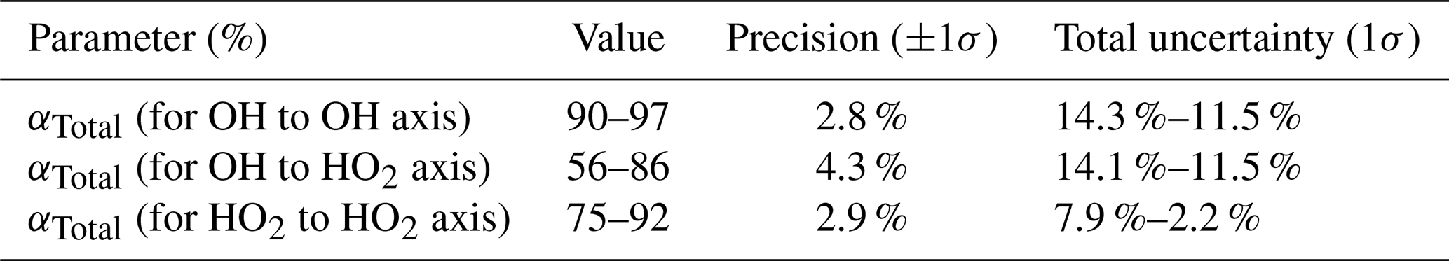
Table 8 shows the measured sensitivity values using APACHE for OH at the first axis (C_OH), OH at the second axis (C_OH(2)), and HO₂ at the second axis ($C_{{\mathrm{HO}}_{\mathrm{2}}}$). The precision denotes the 1σ variability in the measured HO_x signals from HORUS; the total uncertainty is the root sum square of the total uncertainty values from the variables listed in Tables 5 and 6.

Table 8 Pressure-dependent sensitivities for the three measurement within HORUS and their overall uncertainty from calibrations with APACHE. The range in the precision relates to the numbers quoted in the value column.

The undescribed remaining fraction that influences the instrument sensitivity (R_undescribed) is calculated by dividing the overall sensitivity values described in Eq. (4):

$$\begin{array}{}\text{(25)}& {\displaystyle }\begin{array}{rl}& R_{\mathrm{OH}}=\\ & {\displaystyle \frac{C_{\mathrm{OH}}}{\text{c0}\cdot {\mathit{\rho }}_{\mathrm{Int}}\left(P,T\right)\cdot Q_{\mathrm{IF}}\left(P,T\right)\cdot b_{\mathrm{c}}\left(T\right)\cdot \left[{\mathit{\alpha }}_{\mathrm{IPI}\mathrm{OH}}\left(P,T\right)\cdot {\mathit{\alpha }}_{\mathrm{HORUS}\mathrm{OH}}\left(P,T\right)\right]}}\end{array},\text{(26)}& {\displaystyle }\begin{array}{rl}& R_{\mathrm{OH}\left(\mathrm{2}\right)}=\\ & {\displaystyle \frac{C_{\mathrm{OH}\left(\mathrm{2}\right)}}{\text{c1}\cdot {\mathit{\rho }}_{\mathrm{Int}}\left(P,T\right)\cdot Q_{\mathrm{IF}\left(\mathrm{2}\right)}\left(P,T\right)\cdot b_{\mathrm{c}}\left(T\right)\cdot \left[{\mathit{\alpha }}_{\mathrm{IPI}\mathrm{OH}}\left(P,T\right)\cdot {\mathit{\alpha }}_{\mathrm{HORUS}\mathrm{OH}\left(\mathrm{2}\right)}\left(P,T\right)\right]}}\end{array},\text{(27)}& {\displaystyle }\begin{array}{rl}& R_{{\mathrm{HO}}_{\mathrm{2}}}=\\ & {\displaystyle \frac{C_{{\mathrm{HO}}_{\mathrm{2}}}}{\text{c2}\cdot {\mathit{\rho }}_{\mathrm{Int}}\left(P,T\right)\cdot Q_{\mathrm{IF}\left(\mathrm{2}\right)}\left(P,T\right)\cdot b_{\mathrm{c}}\left(T\right)\cdot \left[{\mathit{\alpha }}_{\mathrm{IPI}{\mathrm{HO}}_{\mathrm{2}}}\left(P,T\right)\cdot {\mathit{\alpha }}_{\mathrm{HORUS}{\mathrm{HO}}_{\mathrm{2}}}\left(P,T\right)\right]}}\end{array},\end{array}$$

$$R_{\mathrm{undescribed}}=\left\{R_{\mathrm{OH}};R_{\mathrm{OH}}\left(\mathrm{2}\right);R_{{\mathrm{HO}}_{\mathrm{2}}}\right\},$$

where R_undescribed is a matrix containing the undescribed remaining factors from the three measurements. When plotting R_undescribed against the internal pressure of HORUS, (see Fig. S10), the data scatters ±0.15(1σ) about the average value of 1.02 (±0.23, 1σ calibration uncertainty). This means that (as an upper limit) <2 % of the overall instrument sensitivity is unresolved by the terms described in Eq. (4). Additionally, the 1σ variability of the R_undescribed is 34 % smaller than the uncertainty in the APACHE calibration, meaning that this remaining fraction is declared as neither pressure dependent nor pressure independent.

It is important to note here that all data shown in Fig. 10, with the exception of the pressure-independent sensitivity coefficients, are in relation to temperatures and pressures HORUS experienced during calibrations in the lab. To apply these findings to real airborne measurements, the pressure- and temperature-dependent terms in Eq. (4) are calculated using the temperatures and pressures that are measured within the instrument during flight. The only terms that affect measurement sensitivity and are directly transferable from the calibrations with APACHE to the measurements in flight shown in Eq. (4) are the pressure-independent sensitivity coefficient as they are not subject to change with the large temperature and pressures ranges HORUS experiences when airborne. Figure 11 shows the pressure- and temperature-dependent terms from Eq. (4) characterized for a typical flight that took place during the OMO-Asia 2015 airborne campaign. In Fig. 11, the sensitivity values, limit of detection, transmission values for OH (blue data points) and HO₂ (red data points), and the ambient water mixing ratios (black date points) that occurred during flight 23 are plotted as a function of altitude. During flight, the OH sensitivity ranged from 5.4(±1.2) cts s⁻¹ pptv⁻¹ mW⁻¹ on the ground to 24.1(±5.4) cts s⁻¹ pptv⁻¹ mW⁻¹ at 14 km. The HORUS sensitivity values for HO₂ ranged from 5.5(±1.2) cts s⁻¹ pptv⁻¹ mW⁻¹ and reached an average maxima of 20.5(±4.5) cts s⁻¹ pptv⁻¹ mW⁻¹ at 11.4 km. Above 11.4 km the HO₂ sensitivity decreased with altitude, reaching 19.7(±4.4) cts s⁻¹ pptv⁻¹ mW⁻¹ at 14 km. This drop in HO₂ sensitivity is attributable to the increasing decline in HO₂ transmission inside HORUS as the aircraft flies higher, despite the sensitivity improvements via quenching as the air is becoming drier. The water vapor mixing ratios at 14 km on average are 3 orders of magnitude lower than the average water vapor mixing ratio of 1.5 % at ground level, which greatly suppresses quenching of OH and thus is the main driver for the general increasing trend in the instrument sensitivity towards HO_x as altitude increases. Additionally, Fig. 11 shows that the limit of detection for both OH and HO₂ decrease with increasing altitude. For OH, the HORUS limit of detection is ∼0.11 pptv at ground level and drops to ∼0.02 pptv at 14 km. For HO₂ the limit of detection is ∼1.2 pptv at ground level and drops to 0.23 pptv at 14 km.

Figure 11 In-flight sensitivity curves, limit of detection, and HO_x transmission plotted against altitude for OH (blue data points) and HO₂ (red data points), and the water vapor mixing ratio (black data points) plotted against altitude in kilometers (bottom plot). Data taken from flight 23.

5 Conclusions

The overall goal of this study was to develop and test a new calibration system capable of providing the high flows required by the airborne HORUS system while maintaining stable pressures across the pressure ranges experienced during flight. Such systems are critical to suitably characterize airborne systems (such as a LIF-FAGE measuring HO_x) that have a strong pressure-dependent sensitivity. In addition, this system is purely based on the use of water vapor photolysis, which is a frequently adopted technique for HO_x instrument calibration (Martinez et al., 2003; Faloona et al., 2004; Dusanter et al., 2008). The COMSOL Multiphysics simulations constrained by temperature, pressure, and mass flow measurements demonstrated that air masses at the boundary of the APACHE system do not have sufficient time to expand into the streamlines created by the HORUS sample flow and influence the HO_x content entering HORUS. The largest uncertainties result from constraining the flux (F_β) entering APACHE ($\mathrm{6.37}\pm \mathrm{1.3}\times {\mathrm{10}}^{\mathrm{14}}$ photons cm⁻² s⁻¹, 1σ) and the total uncertainty in the pressure-independent sensitivity coefficients (ranging from 5.6 % to 6.9 %, 1σ). The two actinometrical methods used to derive F_β proved to be in good agreement with a zeta score of 0.59, considering 1σ of their uncertainties. The HORUS transfer standard method yielded an F_β value of $\mathrm{6.9}\pm \mathrm{1.1}\times {\mathrm{10}}^{\mathrm{14}}$ photons cm⁻² s⁻¹ (1σ), and the ozone monitor method yielded an F_β value of $\mathrm{6.11}\pm \mathrm{0.8}\times {\mathrm{10}}^{\mathrm{14}}$ photons cm⁻² s⁻¹ (1σ). Furthermore, the APACHE system enabled the total OH and HO₂ pressure-dependent transmission factors to be characterized as a function of internal pressure. Calculations of HO_x diffusivity to the walls within IPI and the low-pressure regime within HORUS yielded 90 %–97 % for OH transmission to the first detection axis, 56 %–86 % for OH transmission to the second detection axis, and 75 %–92 % for HO₂ transmission to the second detection axis. Future studies with APACHE are planned to expand upon the findings within this paper, with a particular focus on temperature control and on improving operational pressure and flow speed ranges. However, in this study, the APACHE calibration system has demonstrated that, within the lab, it is sufficiently capable of calibrating the airborne HORUS instrument across the pressure ranges the instrument had experienced in flight during the OMO-Asia 2015 airborne campaign. The overall uncertainty of 22.1 %–22.6 % (1σ) demonstrates that this calibration approach with APACHE compares well with other calibration methods described earlier in Table 1. Nevertheless, there is potential for improvement. Accurate calibrations of instruments, particularly airborne instruments that have strong pressure-dependent sensitivities, are critical to acquiring concentrations of atmospheric species with minimal uncertainties. Only through calibrations can the accuracy of measurements be characterized and allow for robust comparisons with other measurements and with models to expand our current understanding of chemistry that occurs within our atmosphere.