the Creative Commons Attribution 4.0 License.
the Creative Commons Attribution 4.0 License.
 | 28 Jan 2020
A reassessment of the discrepancies in the annual variation of δD-H2O in the tropical lower stratosphere between the MIPAS and ACE-FTS satellite data sets
Charlotta Högberg
Farahnaz Khosrawi
Gabriele P. Stiller
Ralf Bauer
Kaley A. Walker
Sylvia Kellmann
Andrea Linden
Michael Kiefer
Norbert Glatthor
Thomas von Clarmann
Donal P. Murtagh
Jörg Steinwagner
Thomas Röckmann
Roland Eichinger
The annual variation of δD in the tropical lower stratosphere is a critical indicator for the relative importance of different processes contributing to the transport of water vapour through the cold tropical tropopause region into the stratosphere. Distinct observational discrepancies of the δD annual variation were visible in the works of Steinwagner et al. (2010) and Randel et al. (2012). Steinwagner et al. (2010) analysed MIPAS (Michelson Interferometer for Passive Atmospheric Sounding) observations retrieved with the IMK/IAA (Institut für Meteorologie und Klimaforschung in Karlsruhe, Germany, in collaboration with the Instituto de Astrofísica de Andalucía in Granada, Spain) processor, while Randel et al. (2012) focused on ACE-FTS (Atmospheric Chemistry Experiment Fourier Transform Spectrometer) observations. Here we reassess the discrepancies based on newer MIPAS (IMK/IAA) and ACE-FTS data sets, also showing for completeness results from SMR (Sub-Millimetre Radiometer) observations and a ECHAM/MESSy (European Centre for Medium-Range Weather Forecasts Hamburg and Modular Earth Submodel System) Atmospheric Chemistry (EMAC) simulation (Eichinger et al., 2015b). Similar to the old analyses, the MIPAS data set yields a pronounced annual variation (maximum about 75 ‰), while that derived from the ACE-FTS data set is rather weak (maximum about 25 ‰). While all data sets exhibit the phase progression typical for the tape recorder, the annual maximum in the ACE-FTS data set precedes that in the MIPAS data set by 2 to 3 months. We critically consider several possible reasons for the observed discrepancies, focusing primarily on the MIPAS data set. We show that the δD annual variation in the MIPAS data up to an altitude of 40 hPa is substantially impacted by a “start altitude effect”, i.e. dependency between the lowermost altitude where MIPAS retrievals are possible and retrieved data at higher altitudes. In itself this effect does not explain the differences with the ACE-FTS data. In addition, there is a mismatch in the vertical resolution of the MIPAS HDO and H2O data (being consistently better for HDO), which actually results in an artificial tape-recorder-like signal in δD. Considering these MIPAS characteristics largely removes any discrepancies between the MIPAS and ACE-FTS data sets and shows that the MIPAS data are consistent with a δD tape recorder signal with an amplitude of about 25 ‰ in the lowermost stratosphere.
- Article
(5233 KB) - Full-text XML
-
Supplement
(429 KB) - BibTeX
- EndNote


The transport of water vapour from the troposphere to the stratosphere through the cold tropical tropopause layer (TTL) is a critical atmospheric process. On the one hand, it directly influences the radiative balance as water vapour is the most important greenhouse gas in this region. On the other hand, it constitutes an important contribution to the water vapour budget in the stratosphere. There are multiple transport pathways. The slow ascent within the ascending branch of the Brewer–Dobson circulation (Brewer, 1949) is thought to be the dominating pathway (Fueglistaler et al., 2009). This ascent is accompanied by large horizontal transport patterns (e.g. Holton and Gettelman, 2001; Bonazzola and Haynes, 2004). They cause a large part of the air trajectories to pass over the western Pacific, where often the lowest temperatures are encountered and consequently the final dehydration is attained. In addition, the convective lofting of ice particles into the stratosphere is thought to be an important pathway (e.g. Moyer et al., 1996; Dessler et al., 2016). Once the ice particles reach the stratosphere they evaporate and enhance the amount of stratospheric water vapour. Overall, the stratospheric water vapour entry mixing ratios amount to only 3.5–4.0 ppmv on an annual average (Kley et al., 2000), which is a reduction of 3 orders of magnitude compared to the mixing ratios commonly observed at the Earth's surface.
The δD-H2O (hereafter simply denoted as δD) isotopic ratio (see Eq. A1) between the minor water vapour isotopologue HD16O (hereafter HDO) and the main isotopologue (hereafter H2O) is a valuable tool for atmospheric research (e.g. Dansgaard, 1964; Kaye, 1987). This is because it is sensitive to physical, chemical and radiative processes, which can be used to infer the history of air parcels. As such it can help to discern the relative importance of slow ascent and convective ice lofting for the transport of water vapour into the stratosphere (Moyer et al., 1996). Several parameters are of interest in the tropical lower stratosphere for these investigations; for example, the absolute value of δD, the slope of the HDO–H2O correlation, any long-term trends in δD or the regularity and the size of its annual variation. The slow ascent into the stratosphere can, to a first order, be idealised as a pure Rayleigh fractionation process. Correspondingly, a δD value of about −900 ‰ for water entering the stratosphere would be expected. Observations, however, show typically δD values between about −700 ‰ and −500 ‰ (e.g. Moyer et al., 1996; Johnson et al., 2001; Kuang et al., 2003; Webster and Heymsfield, 2003; Nassar et al., 2007; Högberg et al., 2019), clearly indicating an importance of other processes like the convective lofting of ice or the mixing of air masses and supersaturation effects.
Based on MIPAS observations from Envisat (Environmental Satellite), Steinwagner et al. (2010) reported a steeper slope for the HDO–H2O correlation than expected from Rayleigh fractionation. Discussing different processes influencing the slope they concluded that convectively lofted ice provides the most plausible explanation for the observed steepening of the slope. In their work Steinwagner et al. (2010) only focused on altitudes between 25 km (∼25 hPa) and 30 km (∼12 hPa). Below 25 km (∼25 hPa), they argued, the MIPAS results are affected by a dependency on the lowermost altitude where retrievals are possible. This lowermost altitude is primarily determined by cloudiness but also aerosols, increasing water vapour absorption and the atmospheric temperature (Steinwagner et al., 2007; Lossow et al., 2011). The link to results at altitudes above occurs through error propagation in the MIPAS global fit retrieval approach (von Clarmann et al., 2003). We will refer to this dependency as “start altitude effect” (see more in Sect. 4.2).
An investigation by Dessler et al. (2016) addressed future trends of water vapour in the tropical lower stratosphere, comparing simulations from chemistry–climate models and a trajectory model. A substantial increase of about 1 ppmv until the end of the 21st century was found. About 50 % to 80 % of this trend could be ascribed to a warming of the TTL in this time period (Dessler et al., 2016). The remainder was attributed to an increase in evaporation of convectively lofted ice. Such a trend would inevitably show up as a trend in the δD ratio. An observational analysis of such a possible change in the past was performed by Notholt et al. (2010), employing almost two dozen balloon-borne observations by the Mark IV interferometer (Toon, 1991), covering the time period between 1991 and 2007 and latitudes from 35 to 65∘ N. They found a small positive trend in the δD values of water entering the stratosphere; however, this trend was not statistically significant. The authors concluded that there was no solid indication that the amount of ice entering the stratosphere had changed.
The annual variation of HDO and H2O in the tropical lower stratosphere is characterised by the atmospheric tape recorder signal (Mote et al., 1996; Lossow et al., 2011). The tropical tropopause (cold point) temperature and its annual variation is imprinted in water vapour. The resulting signal is transported upwards and maintained up to about 30 km (∼12 hPa). For δD, the question of whether there is also such a tape recorder signal found as for HDO and H2O arises. If not, or if the pattern is obviously disrupted, it would indicate the importance of other processes than slow ascent such as the convective ice lofting. The reported observations show different answers to this question. Steinwagner et al. (2010) discussed MIPAS observations and found a pronounced and coherent tape recorder signal in δD up to 30 km (∼12 hPa). Slightly above the tropopause the annual variation had an amplitude of about 60 ‰ to 70 ‰, which is close to the expected variation based on the annual variation of the tropopause temperature. It can be expected that these results are affected by the start altitude effect described above, as they occur below 25 km (∼25 hPa). Nonetheless, the tape recorder signal was robust in multiple retrieval setups. Randel et al. (2012) analysed observations of the ACE-FTS instrument on board SCISAT (Science Satellite) and found a seasonal variation in the lower stratosphere up to 20 km (∼56 hPa) and assigned this to the Asian and American monsoon systems. They excluded the possibility that this annual variation is a tape recorder signal. In addition, the amplitude of the annual variation in δD was considerably smaller than that observed in the MIPAS observations. Recently, Högberg et al. (2019) compared multiple δD data sets from MIPAS, ACE-FTS and the SMR instrument aboard the Odin satellite and concluded that all showed characteristics that typically are associated with the tape recorder signal. They iterated that pronounced quantitative differences exist, which would yield different interpretations of the relative importance of convection for lower stratospheric water vapour.
On the modelling side, Read et al. (2008) derived an amplitude of about 25 ‰ for the annual variation of δD slightly above the tropopause, using a conceptual two-dimensional model incorporating slow ascent, extratropical mixing and convection effects. Eichinger et al. (2015b) implemented HDO into the EMAC (ECHAM/MESSy Atmospheric Chemistry) model and showed a coherent tape recorder signal in δD up to about 27 km (∼19 hPa). Slightly above the tropopause the amplitude of the annual variation in δD amounted to about 20 ‰ (Eichinger et al., 2015b). A sensitivity study showed that the methane oxidation determines the upper end of the tape recorder signal. Methane is much less depleted in deuterium than water vapour upon the entrance of the stratosphere, i.e. δD-CH4 ‰ (Röckmann et al., 2011). The water vapour produced in situ in the lower stratosphere has, therefore, high δD values which overshadow the actual tape recorder signal in the EMAC simulation (Eichinger et al., 2015b).
In this work we reassess the differences in the annual variation of δD in the tropical lower stratosphere between the MIPAS (IMK/IAA) and ACE-FTS data sets. For that, we consider newer data set versions than employed in the studies of Steinwagner et al. (2010) and Randel et al. (2012) and find that the same discrepancies exist. We discuss multiple aspects that could give rise to the observed differences, primarily focusing on the MIPAS data set. The MIPAS results in the altitude range below 25 km (∼25 hPa), which have not been included in scientific analyses so far, are considered in particular. The paper is structured as follows. In the next section we briefly describe the data sets used in this study and how they have been handled. In Sect. 3 we reassess the observational discrepancies by showing the tropical lower stratospheric δD time series and by comparing the amplitudes and phases derived for the annual variation. In Sect. 4 we critically consider possible reasons for the discrepancies between the observational data sets. One focus is on the influence that clouds exert on the MIPAS results. In addition, we show that the MIPAS results are influenced by an artefact originating from different vertical resolutions of the retrieved HDO and H2O data. We demonstrate that the consideration of the MIPAS averaging kernels in the correct way largely removes any discrepancies between the MIPAS and ACE-FTS data sets and confirm a δD tape recorder signal with an amplitude of about 25 ‰ in the lowermost stratosphere. A summary and conclusion of our result will be given in Sect. 5.
In this study we focus on data sets derived from observations of Envisat/MIPAS and SCISAT/ACE-FTS. As noted in the Introduction section, we here employ newer data sets than used in the original works of Steinwagner et al. (2010) and Randel et al. (2012) to reassess the observational discrepancies in the annual variation of δD in the tropical lower stratosphere. As a complement, we show Odin/SMR results to cover the entire observational database from satellites since the new millennium. In addition, also results from the EMAC simulation (Eichinger et al., 2015b) are considered. Below, the data sets are briefly described. For a detailed description of the satellite data sets, the reader is referred to the work of Högberg et al. (2019). After the data set description the data handling is explained.
2.1 Brief data set description
MIPAS was a cooled high-resolution Fourier transform spectrometer aboard Envisat (Fischer et al., 2008). Envisat was launched on 1 March 2002 and performed observations until 8 April 2012, when communication with the satellite was lost. Envisat orbited the Earth 14 times a day on a polar sun-synchronous orbit at an altitude of about 790 km. The Equator-crossing times were 10:00 and 22:00 LT (local time) for the descending and ascending nodes, respectively. MIPAS measured thermal emission at the atmospheric limb covering all latitudes. In this work we employ results that are based on the version 5 calibration from the European Space Agency, and they were retrieved with version 20 of the IMK/IAA processor (von Clarmann et al., 2003). The HDO and H2O data are both retrieved from spectral information between 6.7 and 8.0 µm (1250–1483 cm−1) for spectral consistency and in an attempt to adjust the vertical resolution of H2O to that of HDO (Steinwagner et al., 2010). Correspondingly, the resulting H2O data set differs from the nominal IMK/IAA H2O data set (applied in the studies of Schieferdecker et al., 2015 or Lossow et al., 2017, for example), which uses more H2O-specific microwindows. Overall, the data set covers the time period from July 2002 to March 2004, which is referred to as the full resolution period of MIPAS.
ACE-FTS is one of three instruments aboard the Canadian SCISAT (or SCISAT-1) satellite (Bernath et al., 2005). SCISAT was launched on 12 August 2003 into a high inclination orbit at an altitude of 650 km. This orbit provides a latitudinal coverage from 85∘ S to 85∘ N, but it is optimised for observations at high and middle latitudes. ACE-FTS scans the Earth’s atmosphere during 15 sunrises and 15 sunsets a day from about 5 to 150 km altitude. The vertical sampling varies with altitude, ranging from about 1 km in the middle troposphere via 3 to 4 km at around 20 km to 6 km in the upper stratosphere and mesosphere. As MIPAS, the ACE-FTS instrument performs observations in the infrared. Here, we use ACE-FTS version 3.5 for the time period from April 2004 to November 2014. HDO information is retrieved from two spectral bands: 3.7 to 4.0 µm (2493–2673 cm−1) and 6.6 to 7.2 µm (1383–1511 cm−1). The H2O retrieval uses spectral information between 3.3 and 10.7 µm (937–2993 cm−1).
Odin is a Swedish-led satellite mission that is dedicated to both aeronomy and astronomy observations. Odin was launched on 20 February 2001 into a sun-synchronous orbit with Equator-crossing times of about 06:00 and 18:00 LT on the descending and ascending nodes, respectively. SMR is one of two instruments aboard the Odin satellite and measures the thermal emission at the atmospheric limb (Murtagh et al., 2002). Here, we consider SMR results from the retrieval version 2.1 for the time period December 2001 to May 2009. The use of later data from this retrieval version is not recommended. HDO (H2O) information is retrieved from an emission line centred at 490.597 GHz (488.491 GHz) as described in the work of Urban et al. (2007).
EMAC (v2.42.0; Jöckel et al., 2010, 2016) is a chemistry–climate model which contains the general circulation model ECHAM (Roeckner et al., 2003) and the MESSy (Jöckel et al., 2005) submodel coupling interface. We use the results of a transient EMAC model simulation with a T42 horizontal () resolution with 90 layers in the vertical and explicitly resolved middle atmosphere dynamics (T42L90MA). In this setup, the uppermost model layer is centred at around 0.01 hPa, and the vertical resolution in the upper troposphere lower stratosphere region is between 500 and 600 m. To assure that the meteorological situation largely resembles observational data, newtonian relaxation (“nudging”) towards data of potential vorticity, divergence, temperature and the logarithmic surface pressure from the ECMWF (European Centre for Medium-Range Weather Forecasts) ERA-Interim reanalysis project (Dee et al., 2011) is applied up to 1 hPa. Besides the standard MESSy submodels, the H2OISO submodel (Eichinger et al., 2015a) is used in the simulation. It reproduces the EMAC hydrological cycle with additional consideration of HDO and in all three phases, respectively. For the water isotopologues, equilibrium and kinetic fractionation effects during phase changes in surface fluxes as well as in cloud and convection processes are included (Werner et al., 2011; Eichinger et al., 2015a). In addition to that, Eichinger et al. (2015a) considered H2O and HDO depletion through methane oxidation, which is determined by the mixing ratios of the three oxidation partners (Cl, OH and O(1D)) and the photolysis rate. The deuterium yield in HD is considered using an empirical approach by McCarthy et al. (2004).
2.2 Data handling
In this work we use the “separate” approach for all δD results as defined by Högberg et al. (2019). That means the results (like the time series) are derived separately for HDO and H2O and subsequently combined to δD. The reason for this approach is consistency since the SMR observations of HDO and H2O are not simultaneous, and hence δD cannot be derived on a single profile basis. As shown by Högberg et al. (2019) there are some differences between the different approaches to calculate δD results because of their non-commutativity. However, the main conclusions of this work are not affected by the particular approach chosen. In the Supplement we show a few δD results for the MIPAS and ACE-FTS data sets based on the “individual” approach, i.e. derived from individual δD profiles (see Fig. S4).
The prescreening of the individual satellite data sets is the same as described in Sects. 2 and 3 of Högberg et al. (2019). The time series used in this work are based on monthly and zonal averages considering data in the latitude range from 15∘ S to 15∘ N. Before the data for a specific bin are averaged an additional screening is performed, as described by Eq. (A4) in the Appendix. Subsequently, the data are combined. Averages based on less than 20 observations for SMR and MIPAS data sets, respectively, are not considered any further. For the sparser ACE-FTS data sets, a minimum of five observations is required. In addition, averages that, in absolute values, are smaller than their corresponding standard errors are not further taken into account.
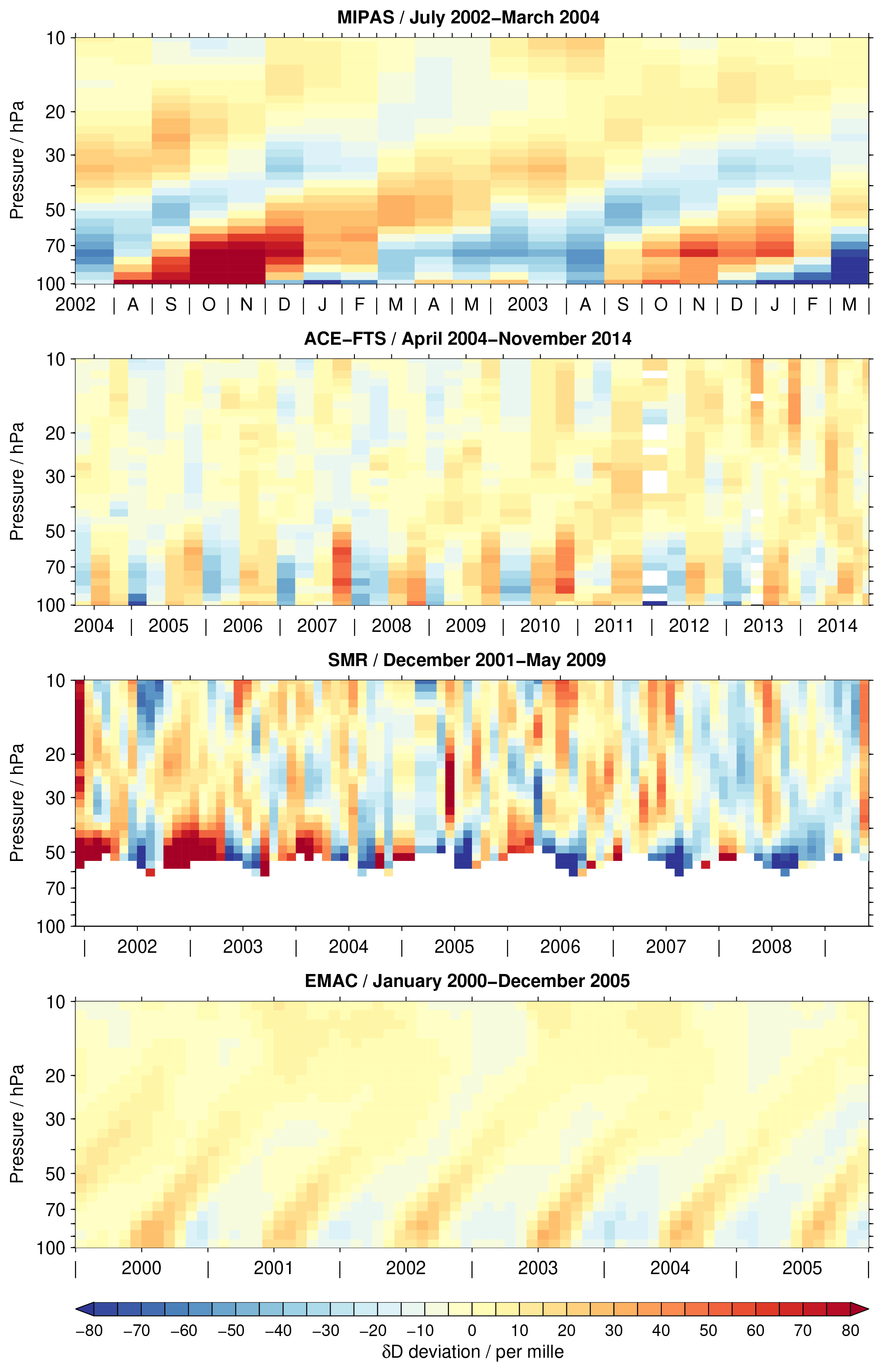
Figure 1Tropical time series of δD deviations from the annual mean covering the altitude range between 100 and 10 hPa. Depending on the data set, a different time period is covered, which is indicated in the individual panel titles. For the EMAC simulation, the time period from 2000 to 2005 is considered arbitrarily. Observational gaps in the data sets are removed for better visibility, in particular for the ACE-FTS data set. A figure without the gap removal is included in the Supplement. White areas indicate that no data are available.
In this section the observational discrepancies in the annual variation of δD in the tropical lower stratosphere between the MIPAS and ACE-FTS data sets are reassessed using three figures. Figure 1 shows the time series of the data sets in the form of contour plots. In Fig. 2 the focus is on the time series at 70 hPa, not only for δD but also HDO and H2O for the sake of attribution. In addition, fits from a regression model to quantify the amplitude and the phase of the annual variation (see Eq. A5 in the Appendix) are presented in this figure. Figure 3 shows subsequently the derived amplitudes and phases for the annual variation, again for δD, HDO and H2O. In all three figures, results from the SMR observations and the EMAC simulation are shown as a complement.
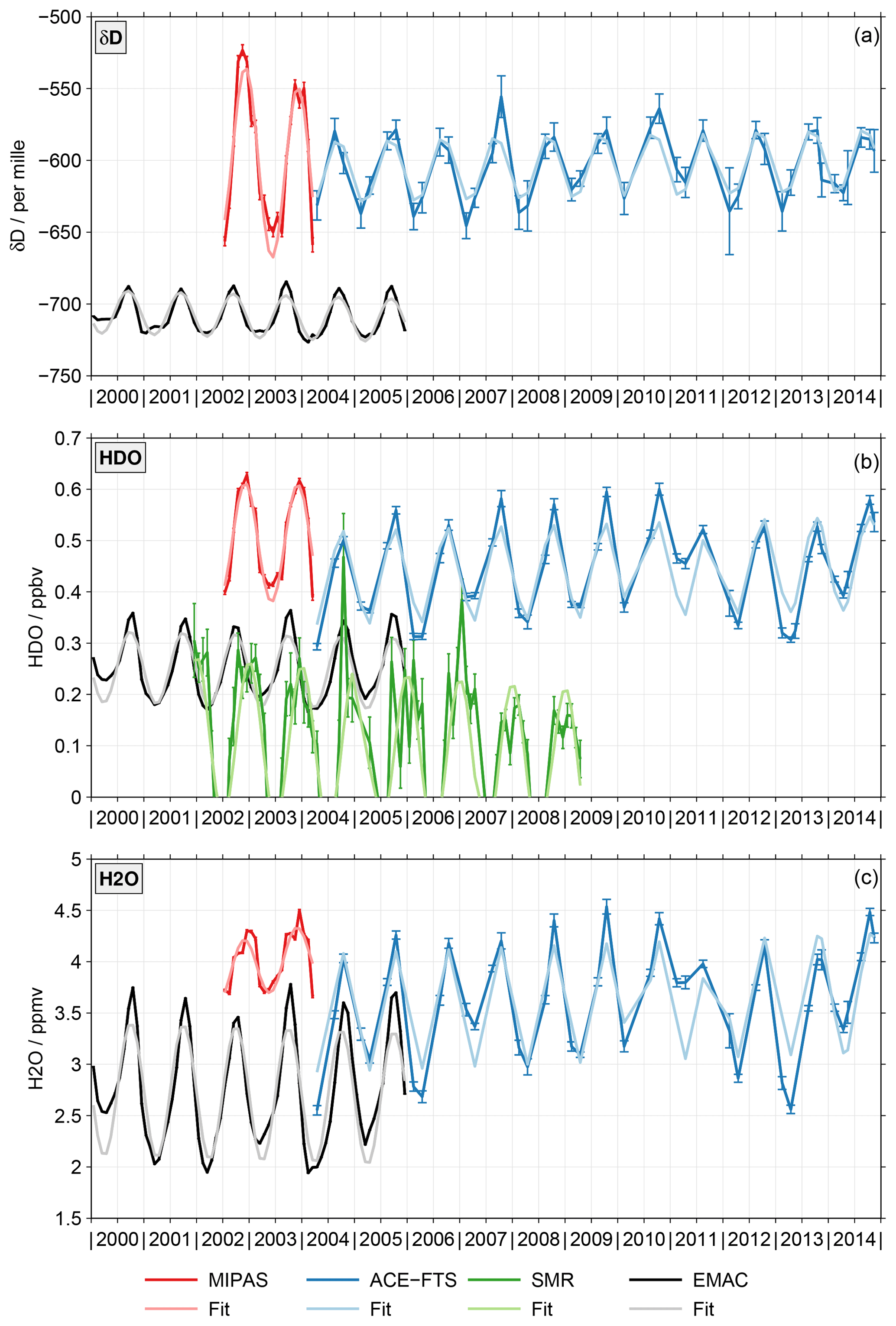
Figure 2Dark colours: monthly mean time series of δD (a), HDO (b) and H2O (c) at 70 hPa for the different data sets. The error bars represent the standard mean errors. Light colours: the fits of these time series based on the regression model described by Eq. (A5).
Figure 1 shows the time series of the δD anomaly with respect to the climatological annual mean for the different data sets. Please note that the time axes vary depending on the data set. For the EMAC simulation, the time period from 2000 to 2005 is arbitrarily considered.
Other time periods change details but not the overall picture. Gaps in the observational time series are removed for visual benefit. This concerns primarily the ACE-FTS data sets that have tropical coverage typically only during four months, i.e. February, April, August and October. In 2013 and 2014 there is also some coverage in May and November due to the shifting orbit of SCISAT. This coverage is limited to the very beginning of these months and comprises the northern tropics in May and southern tropics in November. Due to the gap removal, the individual monthly averages appear to be valid for longer periods of time in the figure. Also for the SMR data set such gaps occur in early 2005 and 2006. A corresponding figure with these observational gaps is provided in the Supplement (Fig. S1). In addition, a figure showing only 2 years of data for the ACE-FTS, SMR and EMAC data sets is supplied (Fig. S2) to provide a more comparable picture to the time coverage of the MIPAS data set.

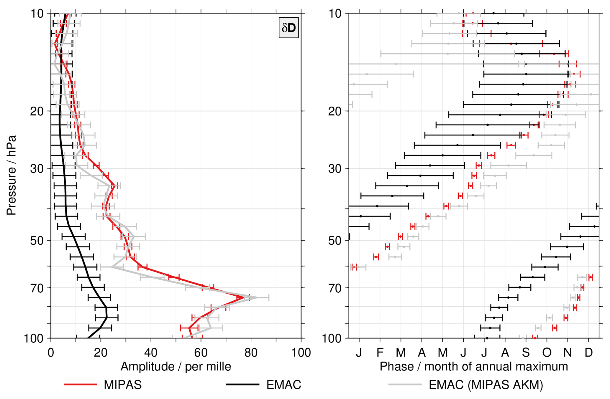
Figure 3Characteristics of the annual variation for δD (a, b), HDO (c, d) and H2O (e, f) in the tropical lower stratosphere as derived from the individual data sets. The left panels show the amplitude and in the right panels the phase is given, expressed by the month where the annual maximum occurs. The error bars represent the 2σ uncertainty level.
The δD results from the different data sets exhibit profound differences. The most coherent temporal behaviour can be observed in the MIPAS data set. It shows a very distinct tape recorder signal in the tropical lower stratosphere, consistent with the results reported by Steinwagner et al. (2010) using an earlier MIPAS retrieval version. Relative to the MIPAS data, the ACE-FTS data set shows a weak annual variation. This is consistent with the results reported by Randel et al. (2012) for the older retrieval version 2.2, where the annual variation was attributed to the monsoon systems. The annual variation is larger below 50 hPa than higher up. The SMR observations provide information on the δD variation roughly above 50 hPa. At lower altitudes no H2O data can be retrieved from SMR measurements of the 489 GHz band. The variation seems to not be very coherent. During some periods, glimpses of a tape recorder signal may be observed, as for example in 2007 and 2008. In contrast, the EMAC simulations show a coherent tape recorder signal which is clearly detectable up to at least 25 hPa. The annual variation is clearly smaller than in the MIPAS data set, fitting much better to that of the ACE-FTS data set.
To characterise the annual variation quantitatively, i.e. its amplitude and phase, we regressed the time series from the individual data sets with a simple regression model that contained an offset, a linear term and the annual variation (see Eq. A5 in the Appendix). The method by von Clarmann et al. (2010) was used to derive the regression coefficients using the standard mean error of the monthly means as statistical weights. Autocorrelation effects and empirical errors as described in Stiller et al. (2012) are not considered for simplicity. As an example, Fig. 2 shows the fits (light colours) of the tropical, monthly mean δD (Fig. 2a), HDO (Fig. 2b) and H2O (Fig. 2c) time series (dark colours) from the different data sets at 70 hPa. In the Supplement a corresponding figure (Fig. S3), focusing on data at 30 hPa, is provided. Figure 3 summarises the derived amplitudes (Fig. 3a, c, e; see Eq. A6 in the Appendix) and phases (Fig. 3b, d, f; see Eq. A7 in the Appendix) as a function of altitude for all data sets. The top row considers the results for δD, while the results for HDO and H2O are shown in the middle and bottom rows, respectively. The error bars indicate the 2σ uncertainty level of the derived quantities. The amplitudes of the annual variation in δD exhibit clear differences between the MIPAS and ACE-FTS data sets up to about 30 hPa. The data sets from both instruments show the largest amplitudes in the lower stratosphere at about 75 hPa. However, at this altitude also the differences between the MIPAS and ACE-FTS data sets maximise (about 50 ‰). This result is affected by the start altitude effect described in the Introduction section. Above, the amplitude decreases significantly. Between 50 and 30 hPa the amplitude for the MIPAS data set is relatively constant, with slightly more than 20 ‰. Slightly below 40 hPa the ACE-FTS data set shows essentially no annual variation, which may be an artefact. However, this behaviour is also observed for the older version 2.2 data set used in the work of Randel et al. (2012), which in addition covers a shorter time period. Higher up, the amplitude increases again to 10 ‰ close to 30 hPa. The SMR data set exhibits a very large amplitude at its lower boundary. It quickly decreases towards 35 hPa where a good agreement with the ACE-FTS data sets can be observed. Above 30 hPa the amplitudes derived from the individual data sets are much closer. The EMAC results compare best to the ACE-FTS results below 30 hPa, even though some important differences exist. The simulation exhibits the maximum amplitude at about 90 hPa, and it does not show a local minimum around 40 hPa as the ACE-FTS observations do. Around 20 hPa the simulation exhibits the best agreement with the ACE-FTS and SMR results.
For all data sets the annual variation exhibits the typical phase progression associated with the tape recorder signal. Only the ACE-FTS data set shows a slightly special behaviour between 60 and 40 hPa. In the lower part the phase is relatively constant, while above 45 hPa the behaviour could be interpreted as a phase jump (even though the uncertainties are fairly large). It clearly relates to the low amplitude of the annual variation. Higher up, the phase progression is again as expected for a tape recorder. While the vertical structure of the phase qualitatively agrees, there are substantial quantitative differences among the data sets, similar to the amplitude of the annual variation. Below 60 hPa the difference between the MIPAS and ACE-FTS data sets typically amounts to 2–3 months. Here, the ACE-FTS data set systematically indicates an earlier occurrence of the annual maximum, comparing better with the EMAC simulation. Also, between 35 hPa and 15 hPa there are clear differences between the MIPAS and ACE-FTS data sets. They range between 1–3 months, with the latter data set again showing a preceding phase. Above 20 hPa the spread among the data sets is quite large (up to 4 months); however, this applies also to the uncertainties of the phase estimates.
The results for the annual variation of HDO qualitatively indicate a good consistency among the data sets. The most obvious quantitative differences between the MIPAS and ACE-FTS data sets occur around 75, 50 and 20 hPa. The SMR data set exhibits distinctively larger amplitudes below 50 hPa than the other data sets, with few exceptions. Above, the SMR results are close to that of the ACE-FTS and EMAC data sets. The amplitude derived from the EMAC simulation is smallest below 60 hPa. Phase-wise the consistency among the data sets is better for HDO than δD; often the differences are within 2 months. The behaviour that the annual maximum occurs earlier in the ACE-FTS data set than the MIPAS data set persists also for HDO. The EMAC phase precedes all other data sets except above 20 hPa.
The smallest spread among the different data sets in terms of the H2O annual variation amplitude is observed above 40 hPa. Below 50 hPa the amplitudes derived from the SMR data set are substantially larger than those from the other data sets. This behaviour is the primary reason for the corresponding differences observed in the δD data. Below 50 hPa there are also significant differences between the MIPAS and ACE-FTS data sets. The differences amount up to 0.4 ppmv and peak close to 85 hPa. Below 70 hPa the ACE-FTS amplitudes are close to those derived from the EMAC simulation. Higher up, the vertical gradient in the amplitude is smaller in the EMAC simulation, leading to clear differences up to about 40 hPa. The comparisons for the phases of the annual variation in H2O largely resemble the results obtained for HDO.
As shown in the last section, the δD time series in the tropical lower stratosphere and the derived characteristics of the annual variation exhibit clear differences among the data sets from the MIPAS and ACE-FTS (as well as SMR) satellite observations (and the EMAC simulation). In the following discussion we investigate more thoroughly possible reasons for the differences in the annual variation of δD in the tropical lower stratosphere, with a clear focus on the MIPAS data set. We will consider the three following aspects:
-
the differences in the MIPAS data set in terms of the temporal sampling of the tropics as well as the inferior vertical resolution relative to the ACE-FTS data set;
-
the start altitude effect, i.e. dependency between the lowermost altitude where MIPAS retrievals are possible and retrieved data at higher altitudes, as described in the Introduction section; and
-
a mismatch in the vertical resolution of the MIPAS HDO and H2O data that are used in the δD calculation.
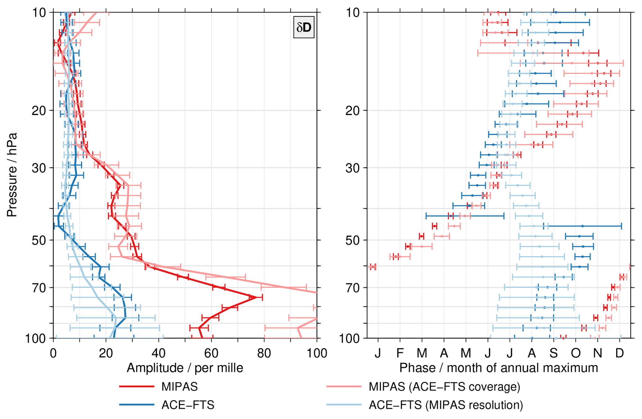
Figure 4As for Fig. 3 but here focusing on test results for δD. Results for a subsampled MIPAS data set that emulates the limited temporal coverage of the ACE-FTS observations in the tropics are shown in light red. The results given in light blue are based on ACE-FTS data whose vertical resolution had been degraded using a Gaussian window with a full width at half maximum of 6 km. The original MIPAS (red) and ACE-FTS (blue) results are shown for comparison.
4.1 Temporal sampling and vertical resolution
There are pronounced differences in the temporal sampling of the tropics between the MIPAS and ACE-FTS measurements. While the sun-synchronous orbit of Envisat yielded a daily coverage of the tropics for MIPAS, the solar occultation measurements of ACE-FTS cover the tropics only at specific times. In general only in February, April, August and October are measurements in this geographical region available (there is some limited observational coverage in May and November in 2013 and 2014). To quantify the impact of this different temporal sampling, we subsampled the MIPAS data to the ACE-FTS coverage. For that, we calculated a mean coverage (day of year versus latitude) of the ACE-FTS observations, separately for sunrise and sunset observations. Only MIPAS observations within ±3 d and of that mean coverage are considered in the subsampled data set. The range in time has been chosen to accommodate the shift of the ACE-FTS coverage over the mission life time as noted in Sect. 3, i.e. a given latitude in the tropics was observed about 3 (6) d later in 2009 (2014) than in 2004. The test results for δD are shown in Fig. 4 in light red. For comparison, the MIPAS (red) and ACE-FTS (blue) results from Fig. 3 are also shown. The results from the subsampled MIPAS data set indicate some systematic effects on the amplitude of the annual variation. Below 60 hPa the subsampled data set actually yields even larger amplitudes, increasing the differences to the ACE-FTS data sets even further. This can be attributed to more obvious differences in HDO than differences in H2O between the two data sets. Around 55 hPa and between about 25 and 15 hPa the subsampling leads to smaller amplitudes typically corresponding to an improved agreement between the MIPAS and ACE-FTS data sets. In terms of the phase the subsampling of the MIPAS data results in larger differences below 70 hPa, while between 30 and 15 hPa an improvement is observed. Due to the subsampling, the error bars of the phase estimates are larger, occasionally leading to an agreement with the ACE-FTS data set in a statistical sense. Overall, the test shows that in some cases agreement improves while in others it becomes worse, clearly indicating that the differences in the temporal sampling between the MIPAS and ACE-FTS data sets are not the main reason for the differences in the annual variation of δD in the lowermost stratosphere.
In terms of vertical resolution the data retrieved from the MIPAS observations have a coarser vertical resolution than the ACE-FTS data. In the altitude region of interest the ACE-FTS data exhibit a vertical resolution between 3 and 4 km. In contrast, the vertical resolution of the MIPAS data used here is between 5 and 6 km. To emulate the vertical resolution of the MIPAS data, the individual ACE-FTS HDO and H2O profiles were smoothed with a Gaussian window that had a full width at half maximum (FWHM) of 6 km. Subsequently, the monthly mean time series were calculated and combined to δD according to the separate approach employed in this work. After that the regression was performed. The results for this test are shown in light blue in Fig. 4. The amplitude of the annual variation is not really affected; typically, there is an agreement with the original results within the error bars. The phases, however, look very different. The characteristics of the tape recorder signal are essentially lost. This applies not only to δD but also to HDO and H2O (not shown). Overall, the test results typically increase the differences between the MIPAS and ACE-FTS data sets. Hence, differences in the vertical resolution between the MIPAS and ACE-FTS data sets can contribute to the observed differences in the annual variation of δD. We will return to this aspect in Sect. 4.3 where we discuss effects of the vertical resolution mismatch between the MIPAS HDO and H2O data. In that section the MIPAS averaging kernels are considered, which, among other data set characteristics, also comprise the vertical resolution.
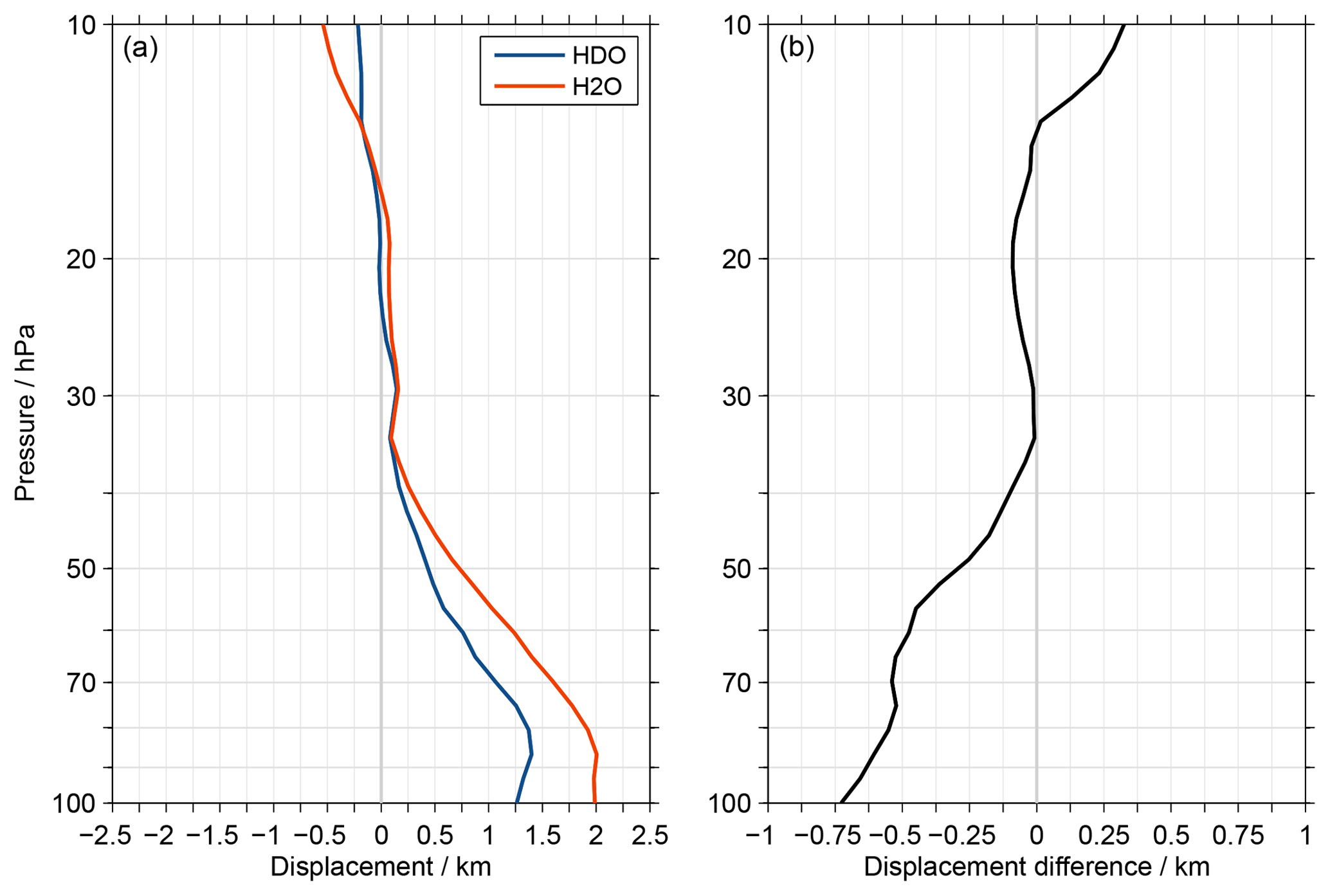
Figure 5(a) The displacement between the MIPAS HDO and H2O averaging kernel peak altitudes and the corresponding retrieval altitudes. (b) The differences between the HDO and H2O displacements.
4.2 The start altitude effect and its impact
The averaging kernel describes various characteristics of a retrieval, like the altitude where the retrieved information originates from or the vertical resolution. An exemplary kernel may peak at the considered retrieval altitude and is symmetric around it. Such behaviour is, however, not observed for the MIPAS retrieval of HDO and H2O in the tropical lowermost stratosphere. Fig. 5a shows the displacement between the averaging kernel peak altitudes and the corresponding retrieval altitudes. These results are based on the average over all retrievals in the latitude range between 15∘ S and 15∘ N. Positive (negative) values indicate that the kernels peak at higher (lower) altitudes than the actual retrieval altitudes. Distinct positive displacements are observed below 35 hPa. In this altitude range the displacements are consistently larger for H2O than HDO. This as also visible in Fig. 5b, which focuses on the differences between the HDO and H2O results. At 100 hPa the displacements between the averaging kernel peak altitudes and the corresponding retrieval altitudes amount to 1.25 km for HDO and 2 km for H2O.
A consequence of this behaviour is the start altitude effect, i.e. dependency between the lowermost altitude where MIPAS retrievals are possible and retrieved data at higher altitudes. They are linked through error propagation in the global fit retrieval approach employed for the MIPAS observations. As such, the effect is not unique to δD, HDO, H2O or the MIPAS retrievals. Due to other characteristics (in terms of constraints, retrieval grid, etc.), this is not an issue for ACE-FTS to our knowledge. Steinwagner et al. (2010) identified the start altitude effect as a potential source of concern regarding their slope results for the HDO–H2O correlation. To avoid related artefacts, they considered slope estimates only in the altitude range between 25 km (∼25 hPa) and 30 km (∼12 hPa). Here, our primary concern is that the start altitude effect has an impact on the annual variation of δD, HDO and H2O in the tropical lower stratosphere (below 25 km). There are two aspects to that.
-
How does the start altitude effect vary during the year?
-
Does the start altitude itself have an annual variation?
To estimate the start altitude effect and its upper boundary, Steinwagner et al. (2010) compared results from two test retrievals:
-
the standard retrieval, where the spectra of the two lowermost tangent altitudes are (intentionally) discarded (Steinwagner et al., 2007); and
-
a test retrieval, where the spectra of the three lowermost tangent altitudes are omitted to emulate a higher start altitude (typically the tangent altitudes are separated by 3 km in the MIPAS observations of this altitude region).
The comparisons of the results from two retrievals (following Eqs. A8 to A11 in the Appendix) showed differences in δD, H2O and HDO up to 25 km (∼25 hPa), similar to the differences seen in Fig. 5. Steinwagner et al. (2010) only considered 200 observations (in February, April, May, June and July) for the analysis of the start altitude effect. To get more robust statistics for all months, we expanded the analysis considerably. Overall, more than 53 000 observations were employed in the additional test retrieval, corresponding to more than 70 % of the tropical observations available in total. Figure 6 shows the differences between the additional test retrieval and the standard retrieval for the individual months.
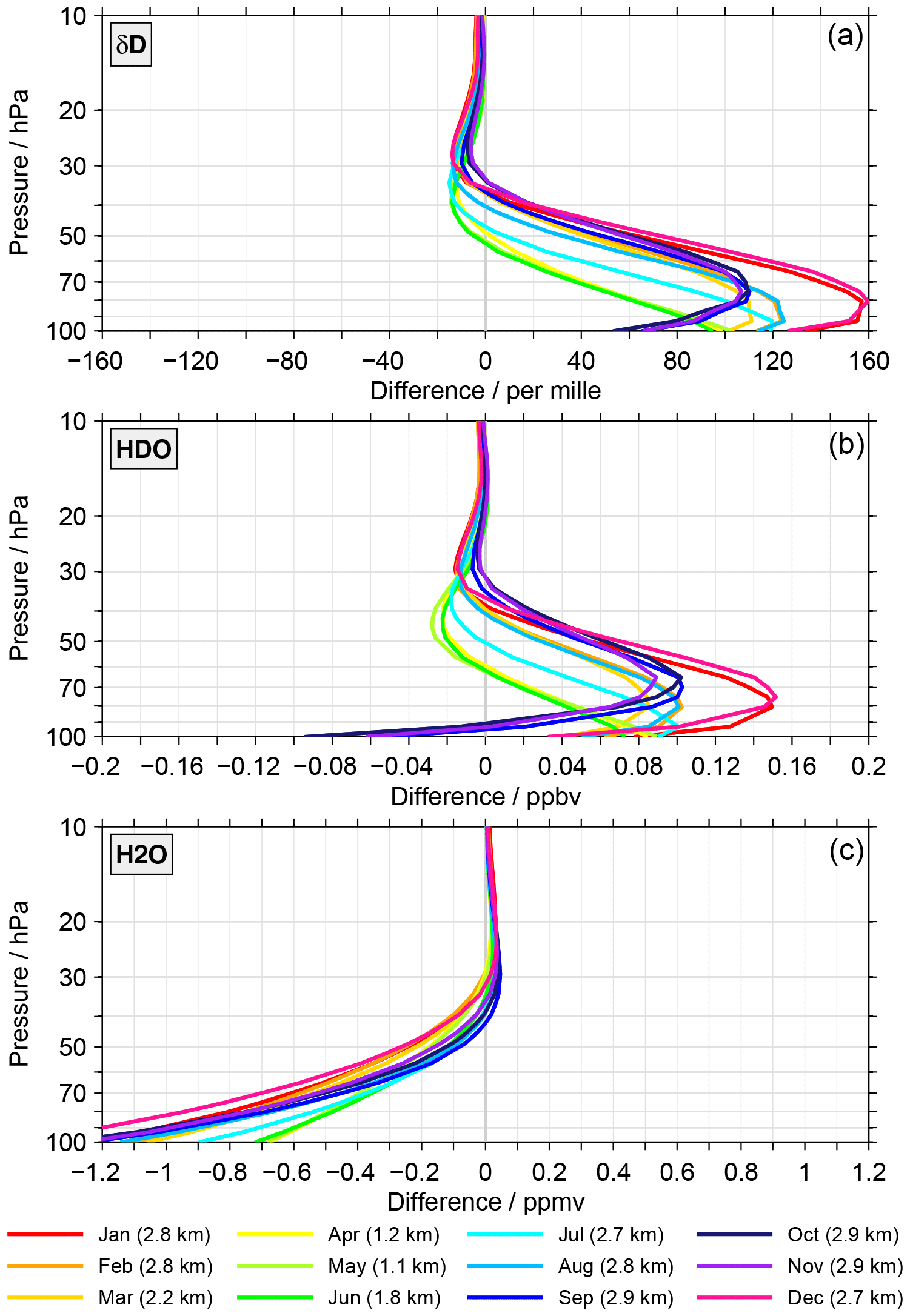
Figure 6Differences in δD (a), HDO (b) and H2O (c) between the test and standard retrieval as a function of altitude and colour-coded for the calendar months. The calculation of these monthly mean differences follows Eqs. (A8) and (A11) in the Appendix. In the legend also the change of the start altitude between the two retrievals is indicated for the individual months, derived according to Eq. (A12).
Considerable differences, i.e. start altitude effects, are observed between the two retrievals. For δD, the differences peak between 100 and 70 hPa. In this altitude range the differences vary between 40 ‰ and 160 ‰. Higher up, the differences decrease in size. Above 50 hPa the differences are typically negative. For HDO, the differences vary within ±0.1 ppbv at 100 hPa. At 70 hPa the differences are entirely positive, ranging from 0.02 to 0.15 ppbv. Higher up, there is, like for δD, again a preference for negative differences. For H2O, the largest differences are observed at 100 hPa, ranging from −1.5 to −0.7 ppmv. Towards higher altitudes the differences become smaller. Above about 40 hPa they are predominantly positive. In general, the start altitude effects become insignificant above 30 hPa, which is consistent with the results presented by Steinwagner et al. (2010). There are some differences between results from Steinwagner et al. (2010) and those presented here. This comprises the size of the differences or transition heights between positive and negative values. Overall, the start altitude effect clearly varies as a function of month and altitude. Also, the change of the start altitude (given in the legend) differs with month. This makes an influence of the start altitude effect on the annual variation of HDO, H2O and δD in the lower stratosphere rather likely.
The question regarding any annual variation of the start altitude itself is answered by Fig. 7. This figure shows the average start altitude for the individual calendar months considering all available HDO data in the latitude range between 15∘ S and 15∘ N. The picture is very similar for the H2O or δD data (using the individual approach). During boreal winter the average start altitude is located around 100 hPa or 16.5 km on the geometric scale. During boreal summer the average start altitude is lower. Overall, the annual variation in the start altitude (maximum minus minimum) amounts to 36 hPa in pressure and 1.85 km in geometric altitude.
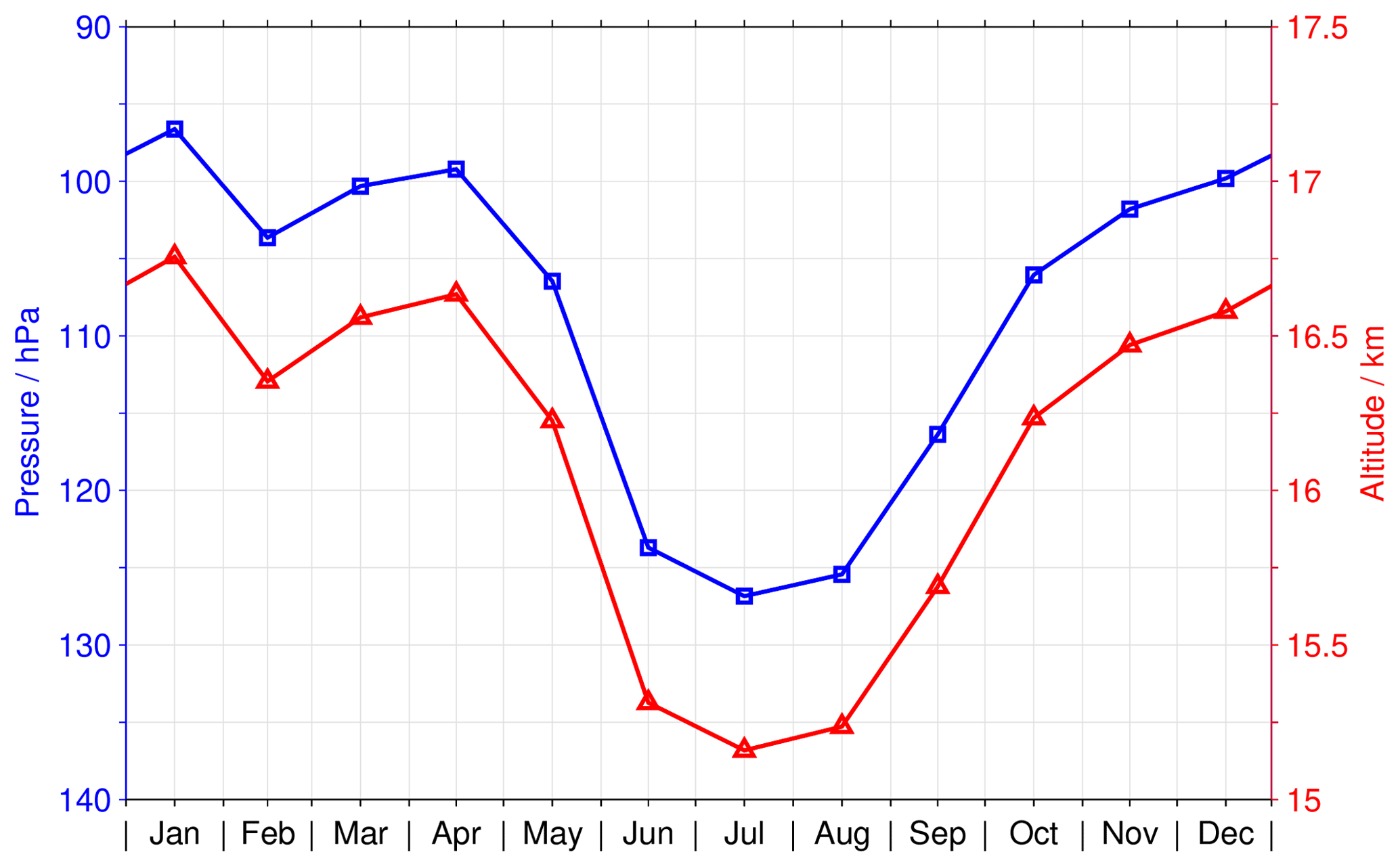
Figure 7The annual variation of the start altitude for the HDO retrieval, i.e. the lowest altitude where sensible data can be derived from the MIPAS observations, considering data in the latitude range between 15∘ S and 15∘ N. The blue line shows the variation in pressure (uses the left axis), and the red line considers the geometric altitude (uses the right axis).
An approximation of the impact of the start altitude effect, in combination with the annual variation of the start altitude, on the annual variation of δD, HDO and H2O is provided in Fig. 8. These estimates were calculated according to Eq. (A15) in the Appendix. However, there are many other possible approaches. The main focus here is on the general distribution of the impact. There are two key points to be taken from this figure:
-
The temporal variation of the impact does not resemble a tape recorder signal. Accordingly, a correction of the MIPAS data for the impact of the start altitude effect will not universally improve the comparisons to the ACE-FTS data set. At some altitudes the comparison of the annual variation in δD will improve while at other altitudes they will deteriorate.
-
The size of the impact is substantial, in particular below 40 hPa. Therefore, the start altitude effect has a profound influence on the amplitude of the δD annual variation derived from the MIPAS data, clearly requiring some caution.
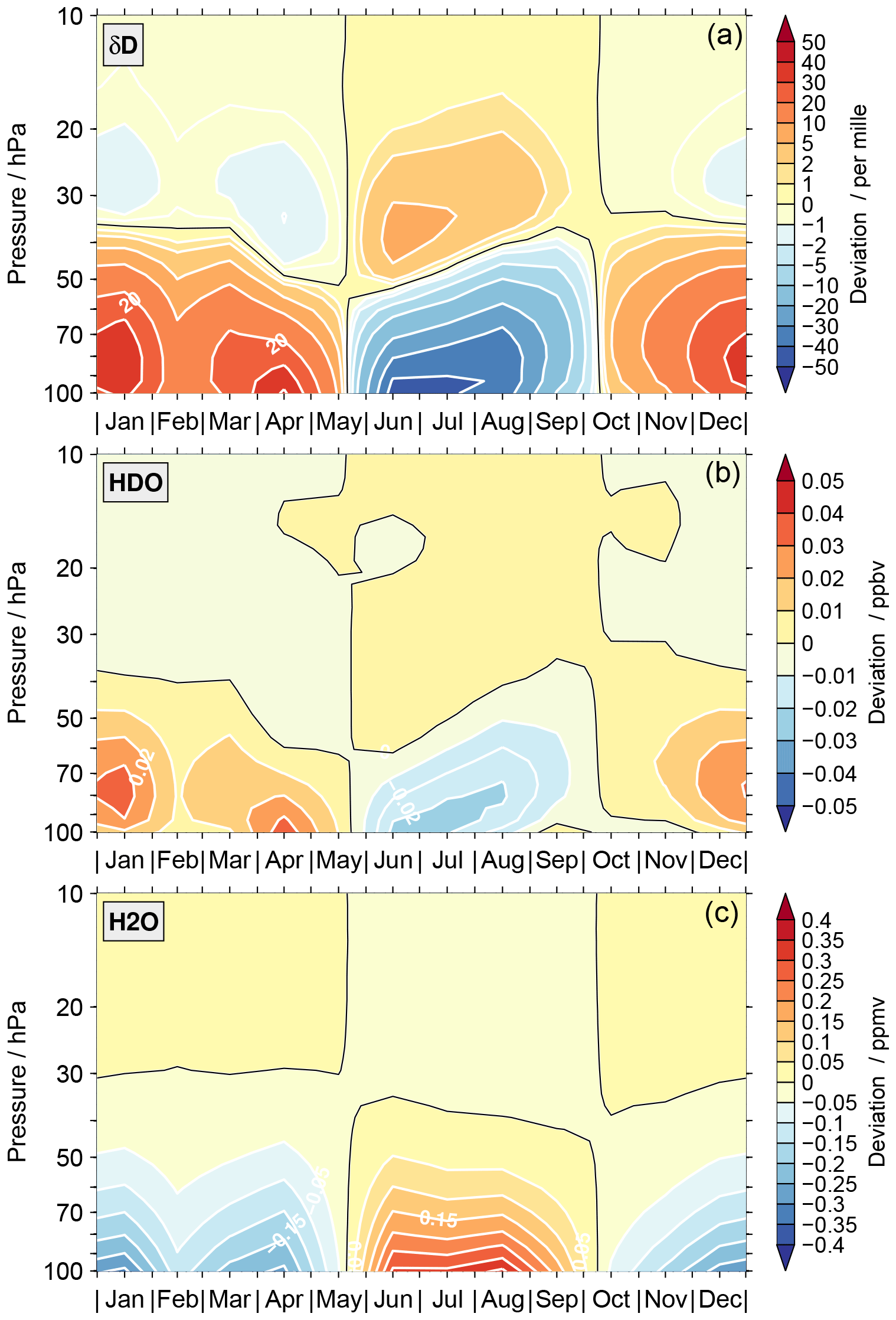
Figure 8The approximated impact of the start altitude effect, in combination with temporal variation of the start altitude, on the annual variation of δD (a), HDO (b) and H2O (c) calculated using Eq. (A15) in the Appendix.
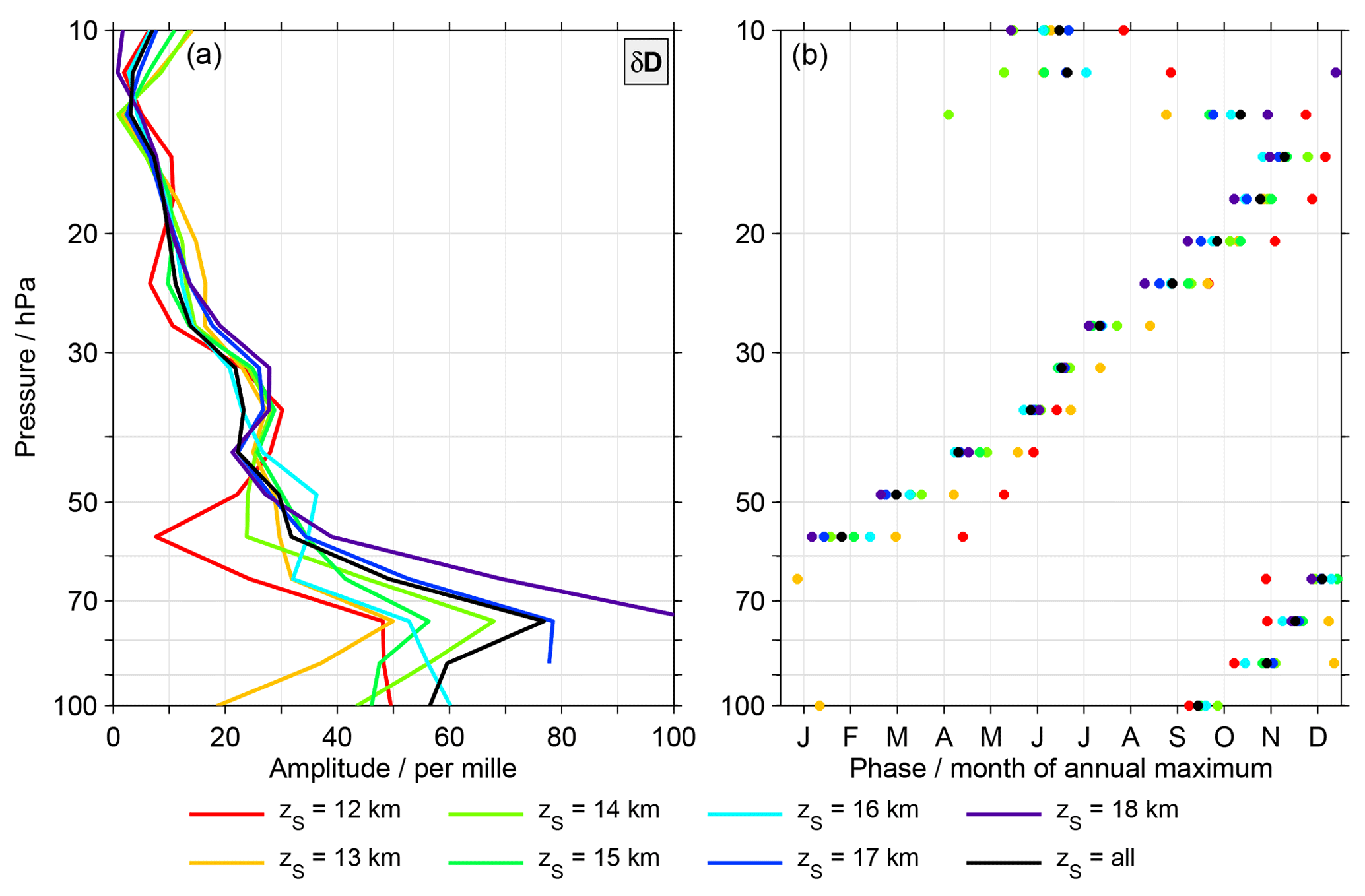
To conclude the discussion of the start altitude effect and its impact, Fig. 9 presents the characteristics of the annual variation in δD for MIPAS data with specific start altitudes. The black line is based on data that incorporate all start altitudes, as shown in Fig. 3. There are differences among the results for different start altitudes. In terms of the amplitude of the annual variation they are most pronounced below 50 hPa. The data combining all start altitudes yields amplitudes that are among the largest, typically only exceeded by the results derived from the data with start altitudes of 17 and 18 km. Phase-wise the differences are typically between 1 and 3 months. Below 60 hPa the data with a start altitude of 12 km often yield the earliest occurrence of the annual maximum. Higher up, the situation is typically reversed. Here, the data with the largest start altitudes show early occurrences of the annual maximum.
Overall, some of the differences observed in Fig. 9 will have natural causes. Data with a start altitude of 12 km relate to more or less cloud-free conditions in the TTL, while data with a start altitude of 18 km represent more cloudy conditions in this altitude region. Nonetheless, for all start altitude scenarios, the amplitudes derived for δD annual variation in the lowermost stratosphere remain larger than for the ACE-FTS observations. Also, for the phases of the annual variation, obvious differences continue to exist. Overall, the start altitude effect clearly impacts the characteristics of the annual variation derived from the MIPAS data, but obviously more aspects are needed to explain the differences between the MIPAS and ACE-FTS data sets.
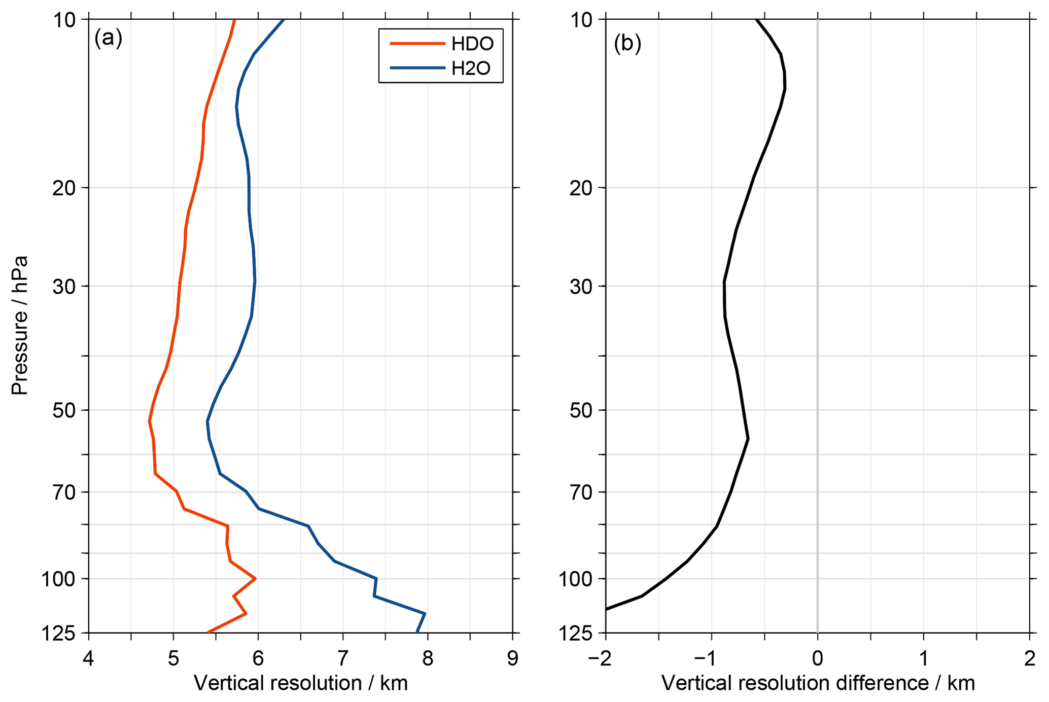
Figure 10 Panel (a) shows the average vertical resolution of HDO (red) and H2O (blue) for the MIPAS data set, considering all tropical observations. The resolution is derived from the averaging kernel rows using the full width at half maximum. The difference between the resolution of HDO and H2O is shown in panel (b).
4.3 Vertical resolution mismatch of the HDO and H2O data
The comparisons of the annual variation in the lowermost stratosphere (Fig. 3) showed a better agreement between the MIPAS and ACE-FTS data sets for HDO than H2O in terms of the amplitude. Also, the displacement between the averaging kernel peak altitudes and the corresponding retrieval altitude shown in Fig. 5 is smaller for HDO than for H2O. This warranted a review of the MIPAS H2O data set, which revealed that its vertical resolution is consistently lower than for HDO in the upper troposphere and lower stratosphere. At 15 hPa the difference is 0.3 km, at 100 hPa about 1.4 km and even more below; this is shown in Fig. 10. The H2O retrieval has been specifically developed for the joint HDO retrieval (Steinwagner et al., 2007), differing from the nominal H2O retrieval approach. The main reason behind this was actually the differences in vertical resolution between the HDO and H2O data, with the latter exhibiting a better resolution. To reduce the vertical resolution of the H2O data, the constraint necessary for a stable retrieval was adjusted. This led, overall, to a better agreement of the vertical resolution of the two species. As such the remaining resolution mismatch can be considered a “residual effect”. In contrast, the retrieval of the ACE-FTS observations are unconstrained (Boone et al., 2013), which by definition leads to the same vertical resolution for HDO and H2O. This mismatch in the vertical resolution of the MIPAS HDO and H2O data can lead to spurious results for δD when they are combined, regardless of whether the combination follows the separate or the individual approach (Högberg et al., 2019). This statement is of general character for any ratio that is not retrieved directly, not only for δD. In addition, it should be noted that this mismatch is inherently also included in the analysis of the start altitude effect and its impact discussed in the previous section. In the following we quantify the impact of this vertical resolution mismatch and show what a correction means for the comparison of the annual variation in δD between the MIPAS and ACE-FTS data sets.
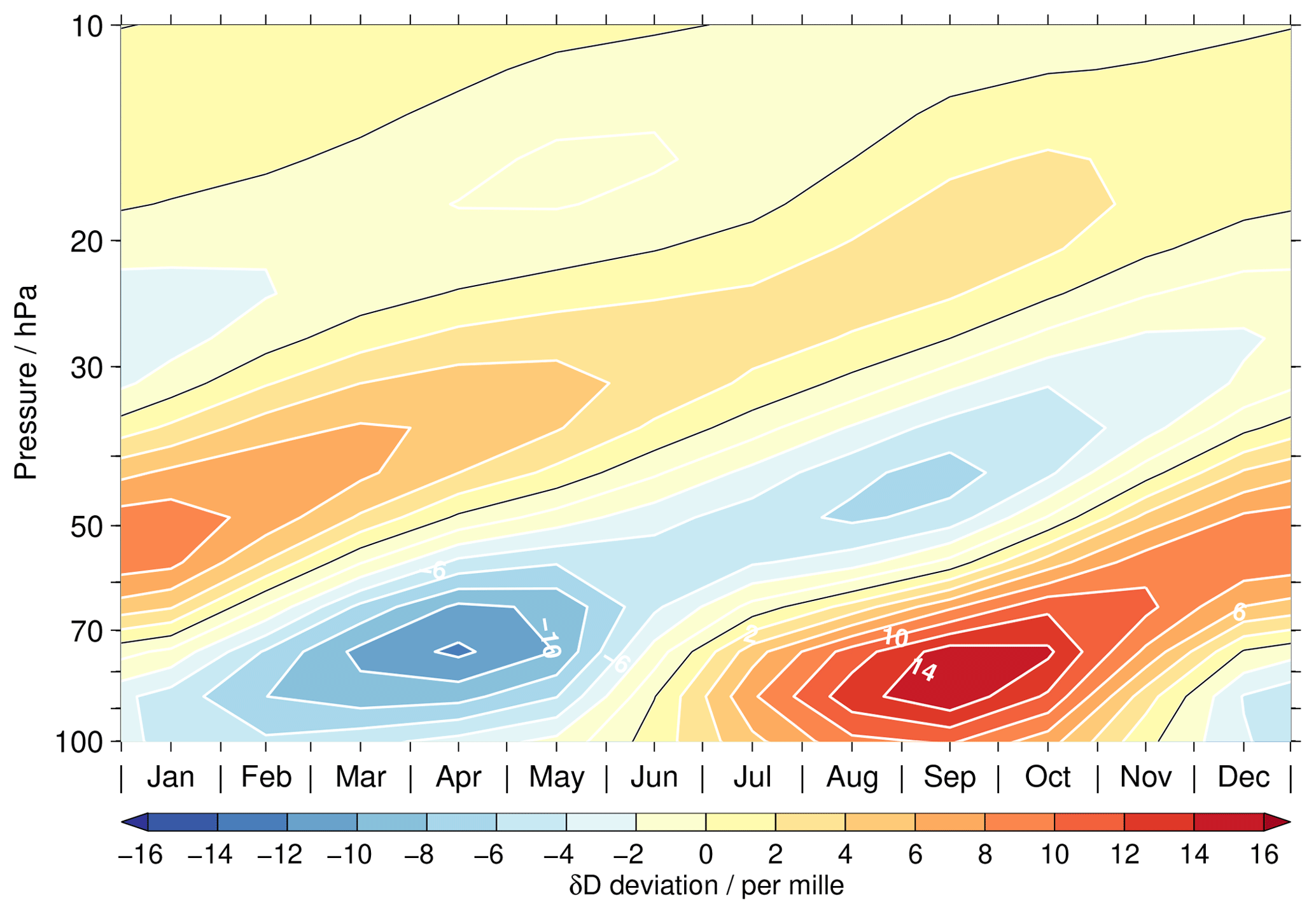
Figure 11 An artificial tape-recorder-like signal in δD due to differences in the vertical resolution of the H2O and HDO data. The results are based on a simple test using the higher vertically resolved EMAC data for the latitude band between 15∘ S and 15∘ N. See text for more details.
4.3.1 Impact
To illustrate the impact of the vertical resolution mismatch, we performed a simple test using the higher vertically resolved EMAC simulation of H2O (see Sect. 2.1). The tropical monthly means were converted to HDO by assuming a constant δD value of −575 ‰ in time and altitude. This constant value roughly corresponds to the overall average value of δD in the tropical lower stratosphere (Nassar et al., 2007; Högberg et al., 2019). Subsequently, the HDO data were smoothed in the vertical domain using a Gaussian window with a FWHM of 5 km to emulate roughly the resolution of the MIPAS HDO data. For H2O, a window with a FWHM of 6 km was used. From the smoothed data a new δD distribution was calculated. The deviations from the annual mean for the resulting δD data are shown in Fig. 11. Due to the mismatch in the vertical resolution of HDO and H2O, the initially time-invariant δD distribution finally exhibits an artificial tape-recorder-like signal. In our simple test this artificial signal has a maximum annual variation of about 14 ‰ close to 80 hPa. Similar results, as described above, were obtained if the conversion of the simulated H2O data to HDO assumed an altitude-varying δD profile (based on ACE-FTS data). Assuming a vertical resolution for H2O of 7 km instead of 6 km increases the amplitude of the artificial tape-recorder-like signal to values between 15 ‰ and 20 ‰, depending on the HDO conversion approach. Overall, the artificial tape recorder signal derived from these simple tests would only explain a part of the differences in the amplitude of the annual δD variation observed between the MIPAS and ACE-FTS data sets. In addition, these simple tests show that the resolution mismatch also influences the slope of the HDO–H2O correlation in the lower stratosphere. Without the mismatch the HDO–H2O slope would be less steep. This includes the altitude range between 25 km (∼25 hPa) and 30 km (∼12 hPa) that was analysed by Steinwagner et al. (2010). Accordingly, the actual slope is closer to the slope predicted for the Rayleigh fractionation process, which is associated with the slow ascent of air into the stratosphere by the upwelling branch of the Brewer–Dobson circulation. The importance of non-Rayleigh processes, as convective ice lofting, is consequently smaller.
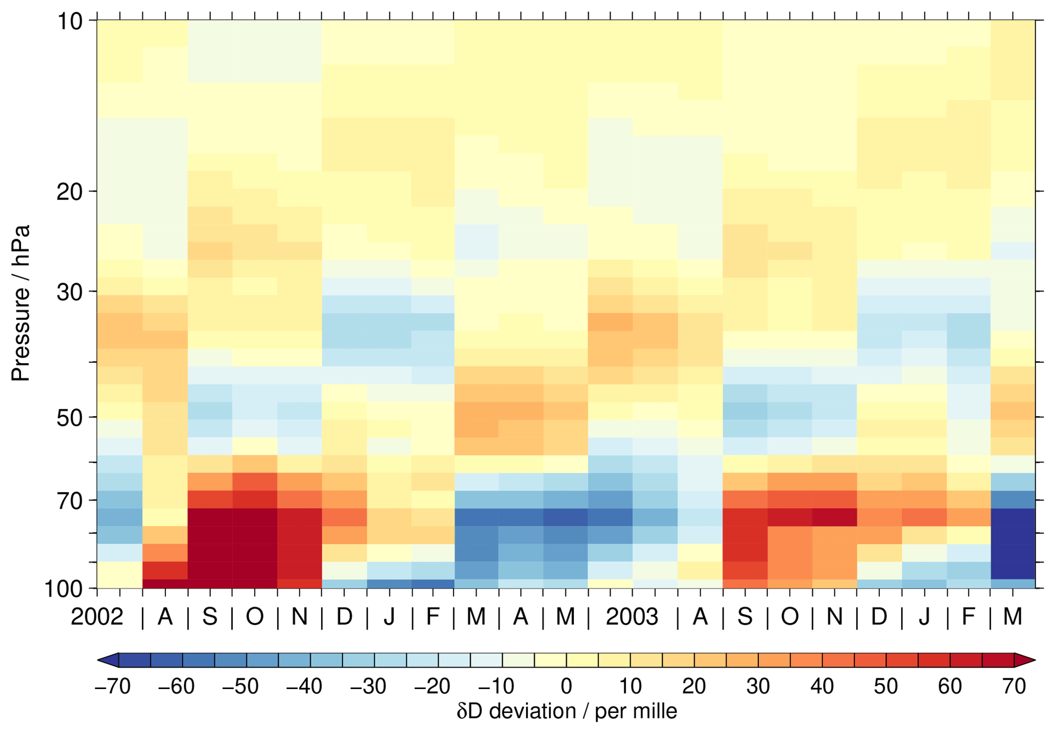
Figure 12An artificial tape-recorder-like signal resulting from the convolution of EMAC data with the MIPAS averaging kernels of HDO and H2O. Again, see the text for more details.
For a more sophisticated study of the effects caused by the resolution mismatch, we involved the actual MIPAS averaging kernels. Unlike in the simple tests above, the kernel shape does not need to have a Gaussian form, and as shown in Fig. 5 they do not need to peak at the actual retrieval altitudes. In addition, the averaging kernels account for the start altitude effect. In this more advanced test we considered the EMAC H2O data for the MIPAS observation period, i.e. from July 2002 to March 2004, again in the form of monthly means for the latitude band between 15∘ S and 15∘ N. As in the simple tests, these data were converted to HDO by assuming a constant δD value of −575 ‰. Then, the monthly means of HDO and H2O were convolved following Eq. (A16) in the Appendix with the corresponding averaging kernel and a priori data taken from the MIPAS data set. For a given month, this convolution considered all tropical MIPAS observations. The number of observations ranges from 2100 to 4400, i.e. one monthly mean model profile was convolved a few thousand times. Involving all MIPAS observations aimed to achieve test results as close as possible to the reality observed by MIPAS. For the same reason, the individually convolved profiles were screened according to the standard MIPAS filtering criteria (see Högberg et al., 2019), appropriate to the individual observations. Subsequently, all convolved and screened profiles in a given month were combined to a monthly mean. Finally, from the combined monthly HDO and H2O data the resulting δD distribution was calculated. The result from this more advanced convolution test is shown in Fig. 12. It exhibits again an artificial tape-recorder-like signal as derived from the simple tests. However there are some distinct differences, which most prominently concern the amplitude of the artificial signal. In September, October and November 2002 the positive deviations amount to around 90 ‰ below 70 hPa, while the negative deviations in March, April and May 2003 range between −55 ‰ and −25 ‰. This means that the characteristics of the MIPAS retrieval yield much larger artificial tape-recorder-like signals as derived from the simple tests, which only focus on the vertical resolution mismatch of the HDO and H2O data but do not include any other aspects covered by the averaging kernels (as asymmetries or the start altitude effect). In addition to differences in the artefact amplitude, there are also differences in the phase. Below 70 hPa the extrema occur about 1 month later in the more advanced convolution test compared to the simple tests shown in Fig. 11. At 50 hPa the delay is about 2 to 3 months and likewise at 25 hPa.
Figure 13Correction of the MIPAS δD data with the results from the convolution test shown in the previous figure. Panel (a) shows the original MIPAS time series and panel (b) the corrected version.
4.3.2 Correction
The artificial tape-recorder-like signal derived from the more advanced convolution test can be effectively used to correct the original MIPAS data. This is shown in Fig. 13 where the original MIPAS data set (Fig. 13a, as in Fig 1) was corrected with the test results shown in the previous figure (Fig. 13b). The annual variation of the corrected δD data is clearly smaller. At 70 hPa the amplitude amounts to 25 ‰ and at 30 hPa to 10 ‰. Both are in agreement with the ACE-FTS data set considering the uncertainties. There are also some phase shifts between the original and corrected time series with respect to the annual variation. This yields both improvements and deteriorations relative to the ACE-FTS data set.
We performed additional advanced convolution tests based on other higher vertically resolved simulations of H2O as well as assuming again an altitude-varying δD profile for the conversion of the simulated H2O data to HDO (see Sect. 4.3.1). For all these tests, the correction of the original MIPAS data consistently yields a pronounced reduction of the amplitude of the δD annual variation. Below 60 hPa the corrected amplitude amounts to about 25 ‰ on average. Higher up, the variation decreases and above 30 hPa it is less than 5 ‰. The corrected phases exhibit a variation of 1 to 2 months, typically. As for the example above, this yields both improvements and deteriorations relative to the ACE-FTS data set.
4.3.3 Further considerations
Overall, the vertical resolution mismatch of the MIPAS HDO and H2O data causes an artificial tape-recorder-like signal. Correcting the original MIPAS data for this artificial signal, using the results from the more advanced convolution tests, shows that the MIPAS tape recorder signal in itself is not entirely artificial. A small signal remains, in good agreement with the ACE-FTS and EMAC data sets. To conclude the discussion on the vertical resolution mismatch and the characteristics of MIPAS averaging kernels, we present results from one more advanced convolution test. In this test the EMAC HDO and H2O data for the MIPAS observation period were taken as they were; i.e. the HDO data were not calculated from H2O assuming a time-constant δD value (see Sect. 4.3.1). On the convolution itself and data handling afterwards nothing was changed. Figure 14 shows correspondingly the characteristics of the annual variation in δD derived from the convolved EMAC data (grey). For comparison, the results from the original EMAC (black) and MIPAS data (red) are shown. The results highlight that the convolution of the EMAC data with the MIPAS averaging kernels actually yields characteristics for the annual variation that are quite similar to those derived from the original MIPAS data itself. This prominently comprises the larger amplitudes and the phase shift to later occurrences of the annual maximum below 50 hPa. This means that the differences between MIPAS and ACE-FTS data sets can only be understood if the characteristics of the MIPAS retrieval, embedded in the averaging kernels, are taken into account. Since the results for the original EMAC data are in relatively good agreement with the ACE-FTS data sets, it can be concluded that also the MIPAS and ACE-FTS data sets are consistent with each other. This echoes the conclusions derived from the correction of the original MIPAS data with the results of the more advanced convolution tests described in Sect. 4.3.2.
Time series of tropical lower stratospheric δD exhibit distinct discrepancies. This concerns in particular the characteristics of the annual variation derived from the MIPAS and ACE-FTS data sets, making it difficult to draw robust conclusions relevant for water vapour transport into the stratosphere. For the amplitude of the annual variation, these differences occur prominently below 30 hPa, with the MIPAS data set consistently indicating larger amplitudes. The maximum difference is observed slightly below 70 hPa where the amplitude derived from the MIPAS data set is about 50 ‰ larger than for the ACE-FTS data set (which shows an amplitude of around 25 ‰). Besides the amplitudes, also the phases of the annual variation exhibit obvious differences between the data sets. In the lowermost stratosphere the differences between the MIPAS and ACE-FTS data sets typically range between 2 and 3 months, with the annual maximum occurring later in the MIPAS data. Around 40 hPa a good agreement is observed, but higher up the comparisons deteriorate again. All data sets (including SMR and EMAC), at least, exhibit the typical phase progression associated with the tape recorder. This is in contrast to the conclusions of Randel et al. (2012) that attributed the annual variation in the ACE-FTS data to the monsoon systems. In this work we find some atypical phase behaviour for the ACE-FTS data set between 60 and 40 hPa, which may hint to other influences or a mixture of different signals. However, higher up, the phase progression is again as expected for the tape recorder.
In this work we considered a number of possible reasons for the observational discrepancies between the MIPAS and ACE-FTS data sets. This comprised, on the one hand, differences in the temporal coverage of the tropics and in the vertical resolution between the two data sets. On the other hand, we investigated impacts of special characteristics of the MIPAS retrieval.
Differences in the temporal coverage of the tropics between the two data sets are not a key factor for the observational discrepancies. The MIPAS data have a lower vertical resolution than the ACE-FTS data. Adapting the ACE-FTS data to this vertical resolution by smoothing them with a Gaussian window (with a FWHM of 6 km) exhibits only little influence on the amplitude of the annual variation of δD. For the phase, this adaption yields an influence, however, that increases the differences between the MIPAS and ACE-FTS data sets.
One characteristic of the MIPAS retrieval is a start altitude effect, i.e. an intercorrelation between the lowermost altitude where sensible retrievals are possible (typically determined by cloudiness) and results at higher altitudes. This effect arises from asymmetric kernels and is, as such, not restricted to the data sets considered in this work nor MIPAS results themselves. The start altitude effect exerts an influence on the δD isotopic ratio and the HDO and H2O volume mixing ratios up to about 30 hPa in the MIPAS retrieval. Besides that, the start altitude itself has an annual variation. Both aspects combined result in a profound impact on the amplitude of the δD annual variation below about 40 hPa. At 100 hPa a crude estimate indicates a contribution to the amplitude of the annual variation of about 40 ‰. The temporal variation of the impact is, however, distinctly different from a tape recorder signal.
The reassessment of the MIPAS data indicated that some of the discrepancies to the ACE-FTS data set may originate from the H2O retrieval, which was specifically set up for the joint analysis with HDO (Steinwagner et al., 2007). It was found that there is a remaining mismatch in the vertical resolution of the MIPAS HDO and H2O data. The resolution of the HDO data is consistently better in the altitude range from 100 to 10 hPa by 0.3 to 1.4 km. Simple convolution tests with the higher vertically resolved EMAC data, adapted so that there is initially no annual variation in δD, show that such a mismatch actually causes an artificial tape-recorder-like signal in δD. We expanded these tests by convolving the model data with the actual MIPAS HDO and H2O averaging kernels and a priori data to obtain realistic results specific to our problem. These tests comprise more MIPAS data set characteristics than just the vertical resolution mismatch and, importantly, also include the start altitude effect and its impact. Also, these tests exhibited artificial tape-recorder-like signals, but they were even more pronounced. After the correction of the original MIPAS data for the artefact, a tape recorder signal still remains but with a reduced size. On average, the peak amplitude amounts to about 25 ‰ in the lowermost stratosphere, in good agreement with the ACE-FTS and EMAC data sets. In the opposite direction, a convolution of the original EMAC data yields characteristics for the annual variation in δD that are quite similar to those derived from the original MIPAS data itself. This considers in particular the larger amplitudes and the direction of the phase shift. Accordingly, the observed differences between the MIPAS and ACE-FTS data sets can be attributed to the characteristics of the MIPAS retrieval (embedded in the averaging kernels) making it essential to consider them.
Finally, both the simple and more advanced convolution tests show that the vertical resolution mismatch in the MIPAS data artificially enhances the slope of the HDO–H2O correlation in the lower stratosphere. This concerns also the altitude range between 25 km (∼25 hPa) and 30 km (∼12 hPa) considered in the work of Steinwagner et al. (2010). Accordingly, the slope is closer to that predicted for the Rayleigh fractionation process and reduces the necessity to involve strong contributions from convectively lofted ice, as was concluded from the original evaluation of the MIPAS dataset (Steinwagner et al., 2010). In a future retrieval version the mismatch in the vertical resolution of the MIPAS HDO and H2O data needs to be fixed.
Within the Appendix we have collected all equations used in this work.
A1 Isotopic ratio
Isotopic ratios are commonly expressed in the delta (δ) notation. δD-H2O (Eq. A1) actually describes the ratio between deuterium (D) and hydrogen (H) in a water sample (Rsample) with respect to a reference ratio (Rreference).
The reference ratio has been defined to be the Vienna Standard Mean Ocean Water (VSMOW; Hagemann et al., 1970).
Based on the approximations that
-
the deuterium content in a sample is dominated by the contribution from HD16O and
-
the hydrogen content essentially comes from ,
Rsample can be written as
A2 Data screening prior the time series calculation
Before the data for a given month in the tropics were averaged they were screened based on the median and median absolute difference (MAD; Jones et al., 2012). Data points outside the interval
were discarded, targeting the most prominent outliers. Here describes the observations (their total number is n) of a given parameter P (i.e. HDO, H2O or δD in the case of the individual approach) at a specific altitude z in the considered month (represented by t).
A3 Calculation of the annual variation characteristics
To characterise the annual variation, i.e. its amplitude and phase, we regressed the time series from the individual data sets with a simple regression model that contained an offset, a linear term and the annual variation:
In the equation denotes the fit of time series for a given parameter P, the time t (in years) and the altitude level z. Coffset(P,z) and Clinear(P,z) are the regression coefficients for the offset and the linear change, respectively. A sine and a cosine with a period pAO of 1 year were used to parameterise the annual variation. The corresponding regression coefficients are and . A more extended regression model, such as considering the semi-annual variation, is not meaningful due to the limited tropical coverage of the ACE-FTS data set. Likewise the MIPAS data set is too short to consider any quasi-biennial oscillation or El Niño–Southern Oscillation (ENSO) variation. To derive the regression coefficients, we followed the method described by von Clarmann et al. (2010). As statistical weights the squared inverse of the standard error of the monthly averages were used. For the sake of simplicity, autocorrelation effects and empirical errors as described in Stiller et al. (2012) are not considered. The amplitude AAO(P,z) of the annual variation is given by
We express the phase PAO by the month in which the annual variation exhibits its annual maximum:
In this equation s(P,z) is a scaling factor which depends on the sign of AAOsigned(P,z). If AAOsigned(P,z) is smaller than zero, then ; if AAOsigned(P,z) is larger than zero, then . The phase derived by Eq. (A7) has a fractional component even though the input data are monthly averages. We kept this fractional component. Correspondingly, no fraction refers to the beginning of a month, while a fraction of 0.5 represents the middle of a month.
A4 Calculation of the start altitude effect
The estimation of the start altitude effect was based on the comparison of results from two retrievals, i.e. the standard and a test retrieval, as described in Sect. 4.2. We denote the former retrieval with the subscript “ref” and the latter retrieval with the subscript “test”. For HDO and H2O (again represented by P), the effect was calculated according to Eq. (A8) below:
Here and describe all results that were available for comparison (i.e. where the start altitude actually changed) in a given month (represented by t), and n is their total number. Exactly the same set of observations were considered from the additional test retrieval and the standard retrieval. In addition, data points missing in one data set (due to the MIPAS filtering) were not considered in the other data set and vice versa. For δD, the start altitude effect was calculated subsequently:
In this equation VSMOW denotes the reference [D]∕[H] ratio expressed by the Vienna Standard Mean Ocean Water, which has been quantified as VSMOW (Hagemann et al., 1970). In practice the differences (and also the start altitudes) were derived on geometric altitudes, which is the basic vertical coordinate of the MIPAS retrievals. Pressure information simultaneously retrieved from MIPAS observations was carried along in the difference calculation, yielding an average pressure profile for a given month. This profile was subsequently used to interpolate the results onto the pressure grid employed here for presentation.
The change of the start altitude zs between the two retrievals, corresponding to Eq. (A8), was calculated as follows:
A5 Calculation of the impact of the start altitude effect
To provide an estimate of the impact I of start altitude effect, in combination with the annual variation of the start altitude, on the annual variation of δD, HDO and H2O (represented by P) we performed the following calculation:
The first part of the equation, i.e. the fraction, relates the changes in δD, HDO and H2O between the additional test retrieval and the standard retrieval to the corresponding changes in the start altitude. As such, this part describes a sensitivity. To estimate the impact I, this sensitivity was applied to the deviation of the start altitude from the standard retrieval in a given month to its overall annual mean (∼16.0 km, see Fig. 7). m is the total number of months considered, i.e. 12. The calculation of the impact for δD uses Δzs(t) and from the HDO data. The estimated impact as such is a crude estimate. Different approaches, for example by a different choice for , will yield different quantitative results for the impact.
A6 Convolution of higher vertically resolved data
The convolution of the higher vertically resolved data (xhigh) onto the vertical resolution of MIPAS (xdeg) was achieved by the equation below, which follows the method of Connor et al. (1994):
Here A and xa priori describe the averaging kernel and the a priori profile of the MIPAS retrieval, respectively.
Data are available upon request.
The supplement related to this article is available online at: https://doi.org/10.5194/amt-13-287-2020-supplement.
The study was initially designed in 2012 by SL, GS, TvC, TR and JS. From 2015 on SL and CH revised and expanded the initial work. Satellite data were provided by RB, KAW, SK, AL, MK and DPM, while the model simulation was provided by RE. The article was written by SL, CH and FK. All co-authors continuously helped with the interpretation and discussion of the results.
The authors declare that they have no conflict of interests.
This article is part of the special issue “Water vapour in the upper troposphere and middle atmosphere: a WCRP/SPARC satellite data quality assessment including biases, variability, and drifts (ACP/AMT/ESSD inter-journal SI)”. It is not associated with a conference.
We would like to thank the European Space Agency for making the MIPAS level-1b data set available. The Atmospheric Chemistry Experiment (ACE), also known as SCISAT, is a Canadian-led mission mainly supported by the Canadian Space Agency (CSA) and the Natural Sciences and Engineering Research Council of Canada (NSERC). Odin is a Swedish-led satellite project funded jointly by the Swedish National Space Board (SNSB), the Canadian Space Agency (CSA), the National Technology Agency of Finland (Tekes) and the Centre National d'Etudes Spatiales (CNES) in France. The Swedish Space Corporation has been the industrial prime constructor. Since April 2007 Odin is a third-party mission of the European Space Agency. Stefan Lossow likes to thank James Dean Bradfield, Nicky Wire, Sean Moore and Richey Edwards for providing the perfect theme for this manuscript: forever delayed. Clearly not a design for life! Also Christopher von Deylen (Ruhe, Schiller!) and André Tanneberger (Silence? What silence? There is no silence!) are acknowledged. We would like to thank three anonymous reviewers for their helpful comments on the paper and the editor Karen Rosenlof.
Stefan Lossow was financially supported by the DFG Research Unit “Stratospheric Change and its Role for Climate Prediction” (SHARP) under contract STI 210/9-2. In addition, he thanks the International Meteorological Institute (IMI) hosted by the Department of Meteorology at Stockholm University for financing multiple visits to Stockholm to work personally together with Charlotta Högberg on this topic. Charlotta Högberg was financially supported by the SNSB project Dnr 88/11 “Atmospheric modelling using space-based observations of stable water isotopes”. She thanks the Bolin Centre for Climate Research for financial support to visit the Karlsruhe Institute of Technology to work on this project.
The article processing charges for this open-access
publication were covered by a Research
Centre of the Helmholtz Association.
This paper was edited by Karen Rosenlof and reviewed by three anonymous referees.
Bernath, P. F., McElroy, C. T., Abrams, M. C., Boone, C. D., Butler, M., Camy-Peyret, C., Carleer, M., Clerbaux, C., Coheur, P.-F., Colin, R., DeCola, P., DeMazière, M., Drummond, J. R., Dufour, D., Evans, W. F. J., Fast, H., Fussen, D., Gilbert, K., Jennings, D. E., Llewellyn, E. J., Lowe, R. P., Mahieu, E., McConnell, J. C., McHugh, M., McLeod, S. D., Michaud, R., Midwinter, C., Nassar, R., Nichitiu, F., Nowlan, C., Rinsland, C. P., Rochon, Y. J., Rowlands, N., Semeniuk, K., Simon, P., Skelton, R., Sloan, J. J., Soucy, M.-A., Strong, K., Tremblay, P., Turnbull, D., Walker, K. A., Walkty, I., Wardle, D. A., Wehrle, V., Zander, R., and Zou, J.: Atmospheric Chemistry Experiment (ACE): Mission overview, Geophys. Res. Lett., 32, L15S01, https://doi.org/10.1029/2005GL022386, 2005. a
Bonazzola, M. and Haynes, P. H.: A trajectory-based study of the tropical tropopause region, J. Geophys. Res., 109, 20112, https://doi.org/10.1029/2003JD004356, 2004. a
Boone, C. D., Walker, K. A., and Bernath, P. F.: Version 3 retrievals for the Atmospheric Chemistry Experiment Fourier Transform Spectrometer (ACE-FTS), The Atmospheric Chemistry Experiment ACE at 10: A Solar Occultation Anthology, A. Deepak Publishing, Hampton, Virginia, USA, 103–127, 2013. a
Brewer, A. W.: Evidence for a world circulation provided by the measurements of helium and water vapour distribution in the stratosphere, Q. J. Roy. Meteor. Soc., 75, 351–363, https://doi.org/10.1002/qj.49707532603, 1949. a
Connor, B. J., Siskind, D. E., Tsou, J. J., Parrish, A., and Remsberg, E. E.: Ground-based microwave observations of ozone in the upper stratosphere and mesosphere, J. Geophys. Res., 99, 16757–16770, https://doi.org/10.1029/94JD01153, 1994. a
Dansgaard, W.: Stable isotopes in precipitation, Tellus, 16, 436–468, https://doi.org/10.1111/j.2153-3490.1964.tb00181.x, 1964. a
Dee, D. P., Uppala, S. M., Simmons, A. J., Berrisford, P., Poli, P., Kobayashi, S., Andrae, U., Balmaseda, M. A., Balsamo, G., Bauer, P., Bechtold, P., Beljaars, A. C. M., van de Berg, L., Bidlot, J., Bormann, N., Delsol, C., Dragani, R., Fuentes, M., Geer, A. J., Haimberger, L., Healy, S. B., Hersbach, H., Hólm, E. V., Isaksen, L., Kållberg, P., Köhler, M., Matricardi, M., McNally, A. P., Monge-Sanz, B. M., Morcrette, J.-J., Park, B.-K., Peubey, C., de Rosnay, P., Tavolato, C., Thépaut, J.-N., and Vitart, F.: The ERA-Interim reanalysis: configuration and performance of the data assimilation system, Q. J. Roy. Meteor. Soc., 137, 553–597, https://doi.org/10.1002/qj.828, 2011. a
Dessler, A. E., Ye, H., Wang, T., Schoeberl, M. R., Oman, L. D., Douglass, A. R., Butler, A. H., Rosenlof, K. H., Davis, S. M., and Portmann, R. W.: Transport of ice into the stratosphere and the humidification of the stratosphere over the 21st century, Geophys. Res. Lett., 43, 2323–2329, https://doi.org/10.1002/2016GL067991, 2016. a, b, c
Eichinger, R., Jöckel, P., Brinkop, S., Werner, M., and Lossow, S.: Simulation of the isotopic composition of stratospheric water vapour – Part 1: Description and evaluation of the EMAC model, Atmos. Chem. Phys., 15, 5537–5555, https://doi.org/10.5194/acp-15-5537-2015, 2015a. a, b, c
Eichinger, R., Jöckel, P., and Lossow, S.: Simulation of the isotopic composition of stratospheric water vapour – Part 2: Investigation of HDO∕H2O variations, Atmos. Chem. Phys., 15, 7003–7015, https://doi.org/10.5194/acp-15-7003-2015, 2015b. a, b, c, d, e
Fischer, H., Birk, M., Blom, C., Carli, B., Carlotti, M., von Clarmann, T., Delbouille, L., Dudhia, A., Ehhalt, D., Endemann, M., Flaud, J. M., Gessner, R., Kleinert, A., Koopman, R., Langen, J., López-Puertas, M., Mosner, P., Nett, H., Oelhaf, H., Perron, G., Remedios, J., Ridolfi, M., Stiller, G., and Zander, R.: MIPAS: an instrument for atmospheric and climate research, Atmos. Chem. Phys., 8, 2151–2188, https://doi.org/10.5194/acp-8-2151-2008, 2008. a
Fueglistaler, S., Dessler, A. E., Dunkerton, T. J., Folkins, I., Fu, Q., and Mote, P. W.: Tropical tropopause layer, Rev. Geophys., 47, RG1004, https://doi.org/10.1029/2008RG000267, 2009. a
Hagemann, R., Nief, G., and Roth, E.: Absolute isotopic scale for deuterium analysis natural waters. Absolute D/H ratio for SMOW, Tellus, 22, 712–715, 1970. a, b
Högberg, C., Lossow, S., Khosrawi, F., Bauer, R., Walker, K. A., Eriksson, P., Murtagh, D. P., Stiller, G. P., Steinwagner, J., and Zhang, Q.: The SPARC water vapour assessment II: profile-to-profile and climatological comparisons of stratospheric δD(H2O) observations from satellite, Atmos. Chem. Phys., 19, 2497–2526, https://doi.org/10.5194/acp-19-2497-2019, 2019. a, b, c, d, e, f, g, h, i
Holton, J. R. and Gettelman, A.: Horizontal transport and the dehydration of the stratosphere, Geophys. Res. Lett., 28, 2799–2802, https://doi.org/10.1029/2001GL013148, 2001. a
Jöckel, P., Sander, R., Kerkweg, A., Tost, H., and Lelieveld, J.: Technical Note: The Modular Earth Submodel System (MESSy) – a new approach towards Earth System Modeling, Atmos. Chem. Phys., 5, 433–444, https://doi.org/10.5194/acp-5-433-2005, 2005. a
Jöckel, P., Kerkweg, A., Pozzer, A., Sander, R., Tost, H., Riede, H., Baumgaertner, A., Gromov, S., and Kern, B.: Development cycle 2 of the Modular Earth Submodel System (MESSy2), Geosci. Model Dev., 3, 717–752, https://doi.org/10.5194/gmd-3-717-2010, 2010. a
Jöckel, P., Tost, H., Pozzer, A., Kunze, M., Kirner, O., Brenninkmeijer, C. A. M., Brinkop, S., Cai, D. S., Dyroff, C., Eckstein, J., Frank, F., Garny, H., Gottschaldt, K.-D., Graf, P., Grewe, V., Kerkweg, A., Kern, B., Matthes, S., Mertens, M., Meul, S., Neumaier, M., Nützel, M., Oberländer-Hayn, S., Ruhnke, R., Runde, T., Sander, R., Scharffe, D., and Zahn, A.: Earth System Chemistry integrated Modelling (ESCiMo) with the Modular Earth Submodel System (MESSy) version 2.51, Geosci. Model Dev., 9, 1153–1200, https://doi.org/10.5194/gmd-9-1153-2016, 2016. a
Johnson, D. G., Jucks, K. W., Traub, W. A., and Chance, K. V.: Isotopic composition of stratospheric water vapor: Implications for transport, J. Geophys. Res., 106, 12219–12226, https://doi.org/10.1029/2000JD900764, 2001. a
Jones, A., Walker, K. A., Jin, J. J., Taylor, J. R., Boone, C. D., Bernath, P. F., Brohede, S., Manney, G. L., McLeod, S., Hughes, R., and Daffer, W. H.: Technical Note: A trace gas climatology derived from the Atmospheric Chemistry Experiment Fourier Transform Spectrometer (ACE-FTS) data set, Atmos. Chem. Phys., 12, 5207–5220, https://doi.org/10.5194/acp-12-5207-2012, 2012. a
Kaye, J. A.: Mechanisms and observations for isotope fractionation of molecular species in planetary atmospheres, Rev. Geophys., 25, 1609–1658, https://doi.org/10.1029/RG025i008p01609, 1987. a
Kley, D., Russell, J. M., and Philips, C.: Stratospheric Processes and their Role in Climate (SPARC) – Assessment of upper tropospheric and stratospheric water vapour, SPARC Report 2, WMO/ICSU/IOC World Climate Research Programme, Geneva, 2000. a
Kuang, Z., Toon, G. C., Wennberg, P. O., and Yung, Y. L.: Measured HDO/H2O ratios across the tropical tropopause, Geophys. Res. Lett., 30, 1372, https://doi.org/10.1029/2003GL017023, 2003. a
Lossow, S., Steinwagner, J., Urban, J., Dupuy, E., Boone, C. D., Kellmann, S., Linden, A., Kiefer, M., Grabowski, U., Glatthor, N., Höpfner, M., Röckmann, T., Murtagh, D. P., Walker, K. A., Bernath, P. F., von Clarmann, T., and Stiller, G. P.: Comparison of HDO measurements from Envisat/MIPAS with observations by Odin/SMR and SCISAT/ACE-FTS, Atmos. Meas. Tech., 4, 1855–1874, https://doi.org/10.5194/amt-4-1855-2011, 2011. a, b
Lossow, S., Khosrawi, F., Nedoluha, G. E., Azam, F., Bramstedt, K., Burrows, John. P., Dinelli, B. M., Eriksson, P., Espy, P. J., García-Comas, M., Gille, J. C., Kiefer, M., Noël, S., Raspollini, P., Read, W. G., Rosenlof, K. H., Rozanov, A., Sioris, C. E., Stiller, G. P., Walker, K. A., and Weigel, K.: The SPARC water vapour assessment II: comparison of annual, semi-annual and quasi-biennial variations in stratospheric and lower mesospheric water vapour observed from satellites, Atmos. Meas. Tech., 10, 1111–1137, https://doi.org/10.5194/amt-10-1111-2017, 2017. a
McCarthy, M. C., Boering, K. A., Rahn, T., Eiler, J. M., Rice, A. L., Tyler, S. C., Schauffler, S., Atlas, E., and Johnson, D. G.: The hydrogen isotopic composition of water vapor entering the stratosphere inferred from high-precision measurements of δD-CH4 and δD-H2, J. Geophys. Res., 109, D07304, https://doi.org/10.1029/2003JD004003, 2004. a
Mote, P. W., Rosenlof, K. H., McIntyre, M. E., Carr, E. S., Gille, J. C., Holton, J. R., Kinnersley, J. S., Pumphrey, H. C., Russell, J. M., and Waters, J. W.: An atmospheric tape recorder: The imprint of tropical tropopause temperatures on stratospheric water vapor, J. Geophys. Res., 101, 3989–4006, https://doi.org/10.1029/95JD03422, 1996. a
Moyer, E. J., Irion, F. W., Yung, Y. L., and Gunson, M. R.: ATMOS stratospheric deuterated water and implications for troposphere-stratosphere transport, Geophys. Res. Lett., 23, 2385–2388, https://doi.org/10.1029/96GL01489, 1996. a, b, c
Murtagh, D. P., Frisk, U., Merino, F., Ridal, M., Jonsson, A., Stegman, J., Witt, G., Eriksson, P., Jiménez, C., Megie, G., de La Noë, J., Ricaud, P., Baron, P., Pardo, J. R., Hauchcorne, A., Llewellyn, E. J., Degenstein, D. A., Gattinger, R. L., Lloyd, N. D., Evans, W. F. J., McDade, I. C., Haley, C. S., Sioris, C., von Savigny, C., Solheim, B. H., McConnell, J. C., Strong, K., Richardson, E. H., Leppelmeier, G. W., Kyrölä, E., Auvinen, H., and Oikarinen, L.: An overview of the Odin atmospheric mission, Can. J. Phys., 80, 309–319, https://doi.org/10.1139/p01-157, 2002. a
Nassar, R., Bernath, P. F., Boone, C. D., Gettelman, A., McLeod, S. D., and Rinsland, C. P.: Variability in HDO/H2O abundance ratios in the tropical tropopause layer, J. Geophys. Res., 112, D21305, https://doi.org/10.1029/2007JD008417, 2007. a, b
Notholt, J., Toon, G. C., Fueglistaler, S., Wennberg, P. O., Irion, F. W., McCarthy, M., Scharringhausen, M., Siek Rhee, T., Kleinböhl, A., and Velazco, V.: Trend in ice moistening the stratosphere – constraints from isotope data of water and methane, Atmos. Chem. Phys., 10, 201–207, https://doi.org/10.5194/acp-10-201-2010, 2010. a
Randel, W. J., Moyer, E., Park, M., Jensen, E., Bernath, P., Walker, K., and Boone, C.: Global variations of HDO and HDO/H2O ratios in the upper troposphere and lower stratosphere derived from ACE-FTS satellite measurements, J. Geophys. Res., 117, D06303, https://doi.org/10.1029/2011JD016632, 2012. a, b, c, d, e, f, g, h
Read, W. G., Schwartz, M. J., Lambert, A., Su, H., Livesey, N. J., Daffer, W. H., and Boone, C. D.: The roles of convection, extratropical mixing, and in-situ freeze-drying in the Tropical Tropopause Layer, Atmos. Chem. Phys., 8, 6051–6067, https://doi.org/10.5194/acp-8-6051-2008, 2008. a
Röckmann, T., Brass, M., Borchers, R., and Engel, A.: The isotopic composition of methane in the stratosphere: high-altitude balloon sample measurements, Atmos. Chem. Phys., 11, 13287–13304, https://doi.org/10.5194/acp-11-13287-2011, 2011. a
Roeckner, E., Bäuml, G., Bonaventura, L., Brokopf, R., Esch, M., Giorgetta, M., Hagemann, S., Kirchner, I., Kornblueh, L., Manzini, E., Rhodin, A., Schlese, U., Schulzweida, U., and Tompkins, A.: The atmospheric general circulation model ECHAM 5. Part I: Model description, Max-Planck-Institut für Meteorologie, Hamburg, Report No. 349, 2003. a
Schieferdecker, T., Lossow, S., Stiller, G. P., and von Clarmann, T.: Is there a solar signal in lower stratospheric water vapour?, Atmos. Chem. Phys., 15, 9851–9863, https://doi.org/10.5194/acp-15-9851-2015, 2015. a
Steinwagner, J., Milz, M., von Clarmann, T., Glatthor, N., Grabowski, U., Höpfner, M., Stiller, G. P., and Röckmann, T.: HDO measurements with MIPAS, Atmos. Chem. Phys., 7, 2601–2615, https://doi.org/10.5194/acp-7-2601-2007, 2007. a, b, c, d
Steinwagner, J., Fueglistaler, S., Stiller, G. P., von Clarmann, T., Kiefer, M., Borsboom, P., van Delden, A., and Röckmann, T.: Tropical dehydration processes constrained by the seasonality of stratospheric deuterated water, Nat. Geosci., 3, 262–266, https://doi.org/10.1038/ngeo822, 2010. a, b, c, d, e, f, g, h, i, j, k, l, m, n, o, p, q
Stiller, G. P., von Clarmann, T., Haenel, F., Funke, B., Glatthor, N., Grabowski, U., Kellmann, S., Kiefer, M., Linden, A., Lossow, S., and López-Puertas, M.: Observed temporal evolution of global mean age of stratospheric air for the 2002 to 2010 period, Atmos. Chem. Phys., 12, 3311–3331, https://doi.org/10.5194/acp-12-3311-2012, 2012. a, b
Toon, G. C.: The JPL MkIV interferometer, Opt. Photonics News, 2, 19–21, 1991. a
Urban, J., Lautié, N., Murtagh, D. P., Eriksson, P., Kasai, Y., Lossow, S., Dupuy, E., de La Noë, J., Frisk, U., Olberg, M., Le Flochmoën, E., and Ricaud, P.: Global observations of middle atmospheric water vapour by the Odin satellite: An overview, Planet. Space Sci., 55, 1093–1102, https://doi.org/10.1016/j.pss.2006.11.021, 2007. a
von Clarmann, T., Glatthor, N., Grabowski, U., Höpfner, M., Kellmann, S., Kiefer, M., Linden, A., Tsidu, G. M., Milz, M., Steck, T., Stiller, G. P., Wang, D. Y., Fischer, H., Funke, B., Gil-López, S., and López-Puertas, M.: Retrieval of temperature and tangent altitude pointing from limb emission spectra recorded from space by the Michelson Interferometer for Passive Atmospheric Sounding (MIPAS), J. Geophys. Res., 108, 4736, https://doi.org/10.1029/2003JD003602, 2003. a, b
von Clarmann, T., Stiller, G., Grabowski, U., Eckert, E., and Orphal, J.: Technical Note: Trend estimation from irregularly sampled, correlated data, Atmos. Chem. Phys., 10, 6737–6747, https://doi.org/10.5194/acp-10-6737-2010, 2010. a, b
Webster, C. R. and Heymsfield, A. J.: Water Isotope Ratios D/H, 18O∕16O, 17O∕16O in and out of clouds map dehydration pathways, Science, 302, 1742–1746, https://doi.org/10.1126/science.1089496, 2003. a
Werner, M., Langebroek, P. M., Carlsen, T., Herold, M., and Lohmann, G.: Stable water isotopes in the ECHAM5 general circulation model: Toward high-resolution isotope modeling on a global scale, J. Geophys. Res., 116, D15109, https://doi.org/10.1029/2011JD015681, 2011. a