the Creative Commons Attribution 4.0 License.
the Creative Commons Attribution 4.0 License.
 | 05 Jun 2020
An improved post-processing technique for automatic precipitation gauge time series
Amber Ross
Alan Barr
The unconditioned data retrieved from accumulating automated weighing precipitation gauges are inherently noisy due to the sensitivity of the instruments to mechanical and electrical interference. This noise, combined with diurnal oscillations and signal drift from evaporation of the bucket contents, can make accurate precipitation estimates challenging. Relative to rainfall, errors in the measurement of solid precipitation are exacerbated because the lower accumulation rates are more impacted by measurement noise. Precipitation gauge measurement post-processing techniques are used by Environment and Climate Change Canada in research and operational monitoring to filter cumulative precipitation time series derived from high-frequency, bucket-weight measurements. Four techniques are described and tested here: (1) the operational 15 min filter (O15), (2) the neutral aggregating filter (NAF), (3) the supervised neutral aggregating filter (NAF-S), and (4) the segmented neutral aggregating filter (NAF-SEG). Inherent biases and errors in the first two post-processing techniques have revealed the need for a robust automated method to derive an accurate noise-free precipitation time series from the raw bucket-weight measurements. The method must be capable of removing random noise, diurnal oscillations, and evaporative (negative) drift from the raw data. This evaluation primarily focuses on cold-season (October to April) accumulating automated weighing precipitation gauge data at 1 min resolution from two sources: a control (pre-processed time series) with added synthetic noise and drift and raw (minimally processed) data from several WMO Solid Precipitation Intercomparison Experiment (SPICE) sites. Evaluation against the control with synthetic noise shows the effectiveness of the NAF-SEG technique, recovering 99 %, 100 %, and 102 % of the control total precipitation for low-, medium-, and high-noise scenarios respectively for the cold-season (October–April) and 97 % of the control total precipitation for all noise scenarios in the warm season (May–September). Among the filters, the fully automated NAF-SEG produced the highest correlation coefficients and lowest root-mean-square error (RMSE) for all synthetic noise levels, with comparable performance to the supervised and manually intensive NAF-S method. Compared to the O15 method in cold-season testing, NAF-SEG shows a lower bias in 37 of 44 real-world test cases, a similar bias in 5 cases, and a higher bias in 2 cases. In warm-season testing, the NAF-SEG bias was lower or similar in 7 of 11 cases. The results indicate that the NAF-SEG post-processing technique provides substantial improvement over current automated techniques, reducing both uncertainty and bias in accumulating-gauge measurements of precipitation, with a 24 h latency. Because it cannot be implemented in real time, we recommend that NAF-SEG be used in combination with a simple real-time filter, such as the O15 or similar filter.
- Article
(2176 KB) - Full-text XML
- BibTeX
- EndNote


Accurate precipitation measurements are crucial for a variety of applications, including water resource forecasting, future water availability, and hydrological and climate analysis and modelling (Barnett et al., 2005; Bartlett et al., 2006; Wolff et al., 2015). Canada's Changing Climate Report led by Environment and Climate Change Canada (Bush and Lemmen, 2019) highlights the importance of accurate precipitation measurements as fundamental climate quantities that play an important role in human and natural systems. Although the systematic bias due to the impact of wind on solid precipitation measurements is well documented (Goodison, 1978; Sevruk et al., 1991, 2009; Goodison et al., 1998; Yang et al., 2005; Smith, 2009; Wolff et al., 2015; Kochendorfer et al., 2017a), errors related to the automatic recording of precipitation measurements have only relatively recently been identified as automated weighing gauges become more commonly used (Sevruk and Chvíla, 2005). The cumulative precipitation data output from automated weighing gauges is subject to noise, diurnal temperature oscillations, and negative drift from evaporation, which can often mean that the precipitation signal over short sampling periods is influenced or hard to detect (Rasmussen et al., 2012). The nature of the noise and drift often varies substantially from site to site and between gauge configurations. High-frequency noise can exceed ±1 mm, and evaporation from the bucket can be in excess of several millimetres between precipitation events. It is therefore necessary to filter the raw data to separate real precipitation events from signal noise and identify and remove periods with evaporation (keeping in mind that evaporation reduces the precipitation amount derived from the differential in bucket weight). Improper filtering can lead to the accumulation of errors and result in significant inaccuracies in total seasonal precipitation. Duchon (2008) suggests that errors due to the diurnal oscillation in Geonor T-200B gauges could be 1 %–10 % of the precipitation total. Three post-processing challenges in the derivation of “clean” precipitation time series are the focus of this study: mechanical and electrical interference, diurnal oscillations, and evaporation of the bucket contents.
This study incorporates two commonly used accumulating automated weighing precipitation gauges (henceforth referred to as automated weighing gauges): the Geonor T-200B and OTT Pluvio2. The Geonor T-200B implements up to three vibrating wire transducers, which provide a frequency output that varies as a function of the fluid weight in the gauge bucket. The cumulative precipitation amount (bucket weight) is calculated from the frequency of each wire via calibration coefficients, with no onboard filtering (Geonor, 2019). The OTT Pluvio2 automated weighing gauge uses a high-precision load cell to weigh the bucket contents and provides several outputs, including intensity and precipitation accumulation (Nemeth, 2008; Nitu et al., 2018). The OTT Pluvio2 output has been pre-processed using an onboard proprietary algorithm which adjusts the high-frequency load cell measurements for temperature and vibration to derive a more accurate bucket weight. Further onboard processing removes the impact of unrealistic bucket-weight changes and evaporation from the output; however, this onboard algorithm was bypassed in this analysis to obtain the data in their rawest form.
A number of post-processing techniques have been developed to derive a noise-free precipitation time series from high-frequency automated weighing-gauge bucket-weight measurements. Some examples are described here.
The rolling maximum filter was used by Harder and Pomeroy (2013) to remove the “jitter” from the accumulated precipitation data sets by retaining a cumulative precipitation observation if it is greater than the previous maximum cumulative precipitation. The previous maximum is assumed to be the cumulative precipitation in all other cases. This filter reportedly works well in preserving the cumulative change in precipitation, but it may not always catch the precise start of precipitation events and will not always perform optimally in the presence of negative gauge drift (i.e. evaporation).
The World Meteorological Organization (WMO) Solid Precipitation Intercomparison Experiment (SPICE, 2013–2015) developed a uniform post-processing method for defining and quantifying precipitation events (Nitu et al., 2018). The process includes calculating a 30 min bucket-weight differential using thresholds and filters, effectively producing what was termed the Site Event Dataset (SEDS). For an event to be identified, the net precipitation duration needed to be sufficiently long (as measured by a precipitation detector or disdrometer), and the total accumulation (as measured by the reference automated weighing gauge) needed to be equal to or greater than a defined threshold (set at 0.25 mm when a reliable precipitation detector was available). This process was effective at creating a high-confidence data set for developing and testing transfer functions (Kochendorfer et al., 2017b) but, because of the rigorous filtering of shorter and smaller events, was not an effective means of filtering a time series.
The US Climate Reference Network (USCRN) uses the redundancy of the Geonor T-200B three vibrating-wire load sensors in the determination of precipitation events (Leeper et al., 2015). Initially, a pairwise calculation was used which relies on pairwise agreement of bucket-weight changes using the wire redundancy as a check on the measurement. This was determined to be sensitive to gauge evaporation and noise, leading to the development of a weighted average calculation using the change in bucket weight between successive sub-hourly periods for each transducer output. A weighted mean is then used to average the bucket weights, with greater weight given to less noisy measurements.
The Meteorological Service of Canada currently implements a real-time threshold filter in their data loggers to automatically determine the occurrence of precipitation events. The filter is based on the 15 min differential in the Geonor T-200B bucket weight (Mekis et al., 2018). Although this filter is unnamed, we call it the operational 15 min filter (O15) automated processing technique. This technique is included in this analysis and is described below in more detail. The filter tends to fail when the noise threshold is exceeded, resulting in false precipitation reports, and when evaporation exceeds the acceptable limits.
Limitations in the O15 technique led to the development of the neutral aggregating filter (NAF), previously known as “Brute Force” (Pan et al., 2016). The NAF, described in greater detail by Smith et al. (2019), iteratively adds all negative and small positive changes to proximate positive changes until all changes exceed a user-specified threshold. Because the technique preserves the total change in bucket weight over the time series, it cannot account for the negative drift that results from evaporation. To overcome this deficiency, the supervised neutral aggregating filter (NAF-S) was created to allow user intervention and minimize evaporation errors through interactive manual adjustment. Both NAF and NAF-S are explained in greater detail in the next section.
To overcome the limitations of the O15, NAF, and NAF-S techniques, we evaluated a moving-window modification of the NAF, implementing the NAF on 24 h overlapping windows, which we will call the segmented neutral aggregating filter (NAF-SEG). The objective was to obtain a robust post-processing technique that is completely automated; easily implemented; and successfully eliminates varying levels of noise, diurnal oscillations, and evaporation without significantly impacting the timing and amount of precipitation. This study introduces the NAF-SEG technique and examines its performance compared to the O15, NAF, and NAF-S methods.
2.1 MSC operational 15 min
The O15 filtering technique is used operationally by the Meteorological Service of Canada (MSC) for Geonor T-200B measurements at the reference climate stations (RCSs). The O15 is implemented in real time at the measurement site data logger. The algorithm is intended to filter out noise and eliminate evaporation while minimizing the reports of false precipitation. For each 15 min period, a mean bucket weight is computed over the last 5 min (minutes 11 to 15) of the period. The mean bucket weight from the initial period is used to establish the baseline. For each successive 15 min period, the difference between the current mean bucket weight and the baseline is calculated. If the bucket-weight difference is greater than or equal to 0.2 mm, the difference is attributed to precipitation and added to the cumulative precipitation total, and the baseline is reset upwards to the current mean. If the difference is less than or equal to −1.0 mm, the difference is attributed to evaporation and the baseline is adjusted downward to match the current mean. This process is performed separately on each of the three installed transducers in the RCS gauge, although ultimately only one is used to determine reported precipitation.
The O15 technique is used operationally in real time and so must be simpler than other post-processing techniques. As a result, it has the potential to be problematic, including a sensitivity to the positive and negative thresholds used to identify precipitation and evaporation events. The 0.2 mm positive accumulating (noise) threshold can cause an overestimation of precipitation if the data are inherently noisy or have a high diurnal oscillation. Additionally, if the negative drift from evaporation lies just above the −1.0 mm threshold, the baseline will not be adjusted before the next precipitation event, resulting in an underestimation of the next event by up to 1.2 mm (evaporation threshold plus the noise threshold).
2.2 Neutral aggregating filter
The NAF method, developed by Environment and Climate Change Canada's Climate Research Division, is an automated method that removes noise from cumulative precipitation time series (Pan et al., 2016; Smith et al., 2019). The processing is done iteratively, beginning with the minimum non-zero interval precipitation value. All non-zero changes in interval precipitation, with values below a user-defined threshold, are transferred to neighbouring periods with positive or larger changes. The results from the algorithm are “neutral”, as the filter balances the positive and negative noise until all changes below the user-defined threshold are eliminated.
The technique removes random noise and accounts for diurnal oscillations in the bucket-weight signal, but, because the total precipitation is forced to equal the total bucket-weight increase at the end of the time series, it cannot account for negative drift. This means that it will not perform well if the time series has significant periods with evaporative losses from the automated weighing precipitation gauge bucket. The significance of the error could exceed 10 % depending on the effectiveness of the servicing measures to reduce evaporation from the bucket contents. NAF serves as the framework for both the NAF-S and NAF-SEG techniques described below.
In this study, the NAF, NAF-S (2.3) and NAF-SEG (2.4) methods all use a minimum threshold P* of 0.001 mm. P* was somewhat arbitrarily set at 0.001 mm based on the minimum resolution of the gauge data. Testing (not shown here) suggests that the method is not overly sensitive to P* and that a 5-fold increase in the magnitude of P* had minimal impact on the performance in either the cold or the warm season.
2.3 Supervised neutral aggregating filter
The NAF-S method is used to manually adjust the cumulative time series for evaporation and other spurious data, effectively reducing the NAF estimation error. The NAF-S method uses the NAF output as a first guess and then allows for manual, interactive adjustment of the baseline to account for evaporation events and other data artifacts impacting the time series. The NAF-S creates an interactive plot, showing both raw (quality controlled) and NAF output data, which highlights periods with drift caused by evaporation. The user is then given the capability to identify and manually exclude each period with evaporation, using the cumulative precipitation value before each evaporation event as a new baseline. NAF-S successfully minimizes the impact of evaporation but requires user intervention (i.e. it cannot be automated) along with user subjectivity to identify the endpoints of evaporative and other spurious events (Smith et al., 2019).
2.4 Segmented neutral aggregating filter
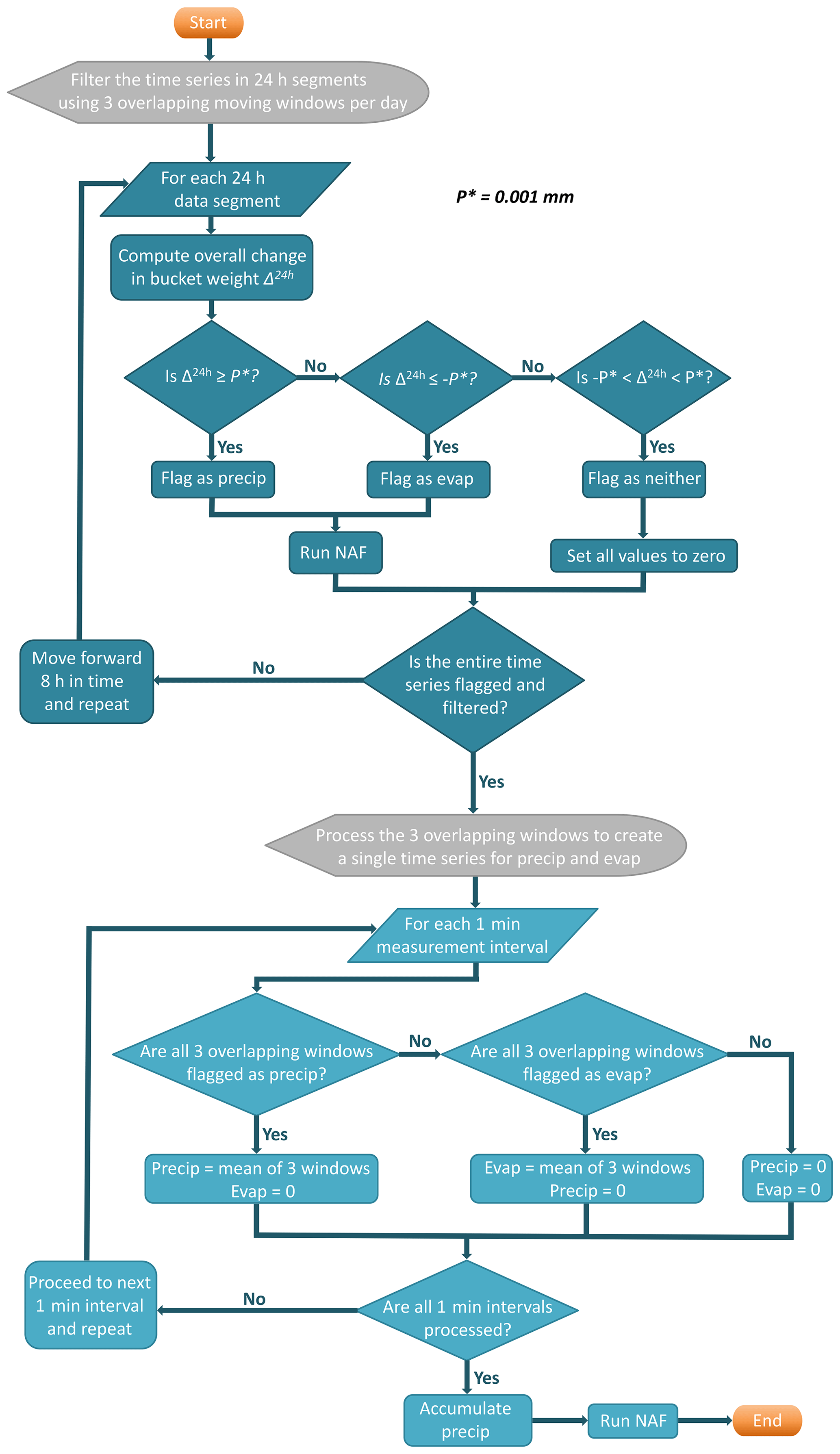
The NAF-SEG is a fully automated technique that implements the NAF to process multi-day precipitation time series in successive 24 h segments using overlapping moving windows. The use of 24 h windows automates the identification and removal of evaporation, minimizing the negative biases in total precipitation from evaporation without the need for user intervention. Additionally, the NAF-SEG method provides an estimate of evaporative losses on precipitation-free days for evaluating servicing procedures. The NAF-SEG technique uses three overlapping moving windows per day, advanced in increments of 8 h. The algorithm begins by filtering the first 24 h segment using NAF. It then advances 8 h and filters the next 24 h segment. This filtering process is repeated until the end of the data is reached. Each 8 h data segment thus passes through the NAF three times. The processing steps are listed below and outlined in Fig. 1.
The measurement interval used in this analysis to evaluate NAF, NAF-S, and NAF-SEG is 1 min. This interval is used here because it was chosen as the preferred interval for archiving of the SPICE data. NAF has been shown to work on data of larger intervals (i.e. 30 min in Pan et al., 2016), and there is no reason why NAF-SEG could not be used with larger intervals as well, provided that the intervals are considerably shorter than the 24 h window (i.e. 30 min or less).
We will denote the precipitation amount from one measurement interval (i) as P(i), cumulative precipitation as cumP(i), evaporation from one measurement interval as E(i), and cumulative evaporation as cumE(i). All units are in millimetres.
-
The time series is processed in successive 24 h segments.
-
For each 24 h segment, the change in bucket weight, which we will call Δ24 h, is computed as the difference between the final and initial observations.
-
Based on the value of Δ24 h, the 24 h segment is assigned one of three states: (1) precipitating, (2) evaporating, or (3) neither. It is then processed accordingly:
- a.
If , the 24 h segment is flagged and treated as a precipitation period with no evaporation. The 24 h segment is passed through the NAF, resulting in values of P(i) that are either zero or greater than or equal to P*.
- b.
If , the 24 h segment is flagged and treated as an evaporation period with no precipitation. The 24 h segment is passed through the NAF but with the sign of the data reversed, resulting in values of E(i) that are either zero or less than or equal to .
- c.
If < Δ24 h < P*, the 24 h segment is flagged as free of both precipitation and evaporation, and all values of P(i) and E(i) are set to zero.
- a.
-
The NAF P(i) and E(i) outputs from step (3) as well as the flags that indicate the presence of precipitation or evaporation are added to arrays with three columns, corresponding to the three overlapping windows per day (i.e. as P(i,j), E(i,j), and flag(i,j), where j denotes columns – windows – 1 to 3).
-
Steps (2) to (4) are repeated using moving windows on successive 24 h segments, beginning 8 h apart, until the entire time series has been processed.
-
The P(i,j) and E(i,j) arrays from steps (3) to (5), with three overlapping windows, are processed to create a single time series for P(i) and E(i), based on the flag.
- a.
For intervals when the flag from all three overlapping windows indicates the presence of precipitation, E(i) is set to zero and the three P(i,j) values are averaged to produce P(i); otherwise P(i) is set to zero.
- b.
For intervals when the flag from all three overlapping windows indicates the presence of evaporation, P(i) is set to zero and the three E(i,j) values are averaged across columns to produce E(i); otherwise E(i) is set to zero.
- c.
For intervals which do not precipitate (6a) or evaporate (6b), i.e. when the flag from all three overlapping windows indicates the absence of both precipitation and evaporation, or when the three flags do not agree with each other, P(i) and E(i) are set to zero.
- a.
-
The P(i) and E(i) outputs from step (6) are summed to create the cumP and cumE time series. Lastly, cumP is passed through the NAF to ensure that all P(i) values are either zero or greater than or equal to P*; cumE is passed through the NAF but with the sign of the data reversed to ensure that all E(i) values are either zero or less than or equal to . The evaporation estimate is taken as the absolute value of the cumulative total of cumE.
Two additional steps not shown in Fig. 1 are required. First, additional 24 h segments need to be added to the start and end of the time series to ensure that all core intervals are covered by three overlapping windows. Since these time series begin at 0 mm at the start of the season, the 24 h segment added to the start of each time series is set to all zero values. The 24 h segment added to the end of the time series is set to the maximum of the cumulative time series. This step is only necessary if the user requires processed data from the first and last 24 h period in the time series and does not impact the precipitation amounts.
A second step is required to ensure that the precipitation during data gaps is not omitted from the accumulated total. Note that when gaps occur in an automated weighing-gauge time series, the total accumulation across the gap is preserved but the event timing is lost. In the NAF-SEG implementation, precipitation occurring over data gaps is preserved if all three windows capture the jump in the bucket weight over the gap. But this will not always be the case. We resolved the problem as follows. First, we identified data gaps that overlapped the start or end of each 24 h segment, computed the difference in bucket weight across the gap, and flagged windows when the difference was greater than or equal to P*. For those segments only, we added a processing step between steps (5) and (6) as follows. If any of the three overlapping windows captured the jump in the bucket weight across the gap, the window or windows in P(i,j) that did not capture the jump were excluded from the averaging, and all three windows were flagged to indicate the presence of precipitation. If none of the windows captured the jump in bucket weight across the gap, the difference across the gap was assigned to the final interval of the gap in P(i,j) for all three windows, with all windows flagged to indicate the presence of precipitation.
Two data sources, both with 1 min resolution, were used to evaluate the O15, NAF, NAF-S, and NAF-SEG precipitation filters: a control (pre-processed) precipitation time series which is free of noise and drift and raw (minimally filtered) automated weighing-gauge data collected at a number of international sites, which contain varying levels of noise, diurnal oscillations, and evaporative drift. The control, pre-processed time series were used to evaluate all four filters – by adding synthetic noise, diurnal oscillations, and evaporative drift and then evaluating the ability of the filters to recover the original time series. The raw time series, following quality control procedures, were passed through each of the filters, and the supervised NAF-S output was used as the standard against which to evaluate the others.
Both data sources, raw data with real-world noise and control data with synthetic noise added, have advantages and disadvantages in assessing filter performance (Peters et al., 2014). Clean data with added noise provide a known “true” control but add the risk that the added noise and drift may not adequately capture the characteristics of real-world measurements. Raw measurements preserve observed noise patterns and capture the variability in noise behaviour across sites and instruments but do not provide a control time series for filter evaluation. By using both complementary data sources, we exploit their respective strengths and thus better assess the relative effectiveness of each filter.
3.1 Testing with pre-processed (control) precipitation data
The pre-processed 1 min cumulative time series was originally derived from an Alter-shielded Geonor T-200B precipitation gauge at Caribou Creek, Canada, from October 2013 to September 2014. It was broken into two seasons to better assess filter performance differences between the cold season (October–April) and the warm season (May–September). The raw gauge outputs were filtered using NAF-S, resulting in a cold-season precipitation total of 259 mm and a warm-season precipitation total of 282 mm. Historically, this particular gauge has performed well with minimal noise (< ±0.25 mm) and evaporation issues; the time series was very clean even prior to filtering, and therefore the filtered output provides a suitable control.
To evaluate the four filters, we added synthetic noise and drift to the filtered (noise-free) control and then tested each filter's ability to recover the original signal. The perturbations included synthetic evaporation, diurnal oscillations, and random noise, computed as follows.
-
Negative evaporative drift was added that totaled 25.9 and 28.2 mm in the cold and warm seasons respectively, or 10 % of the precipitation totals. The synthetic evaporation was partitioned among the 1 min intervals, assuming that interval evaporation was proportional to the vapour pressure deficit (VPD). The fraction of evaporation for each interval was calculated by dividing the interval VPD by the VPD sum over the entire time series. Those fractions were then multiplied by the total (25.9 or 28.2 mm), and the resulting cumulative sum was subtracted from the control cumulative precipitation.
-
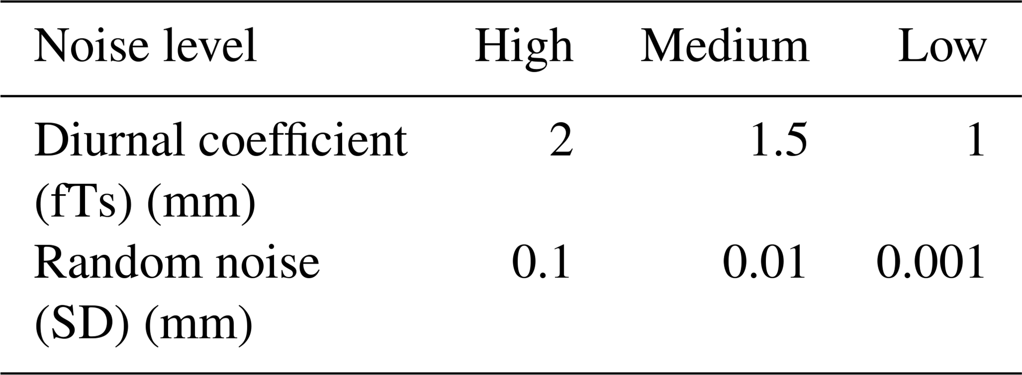
Temperature-dependent diurnal oscillations δT(i) were computed from observed air temperature at gauge height and added to the cumulative precipitation control. The diurnal oscillations were calculated as follows:
where fTs is a coefficient that varies for the different noise scenarios (Table 1). The temperature-oscillation time series δT was then subtracted from the cumulative time series from step (1).
-
Normally distributed random noise was generated for each 1 min interval, with a mean of zero and a specified standard deviation (Table 1). Because the synthetic noise time series is generated randomly, it does not necessarily sum to zero. To avoid adding bias, we forced the sum to zero by subtracting the mean. The result was then added to the cumulative time series from step (2).
The artificially noisy time series from step (3) were adjusted to a value of zero at the start and then filtered using the O15, NAF, NAF-S, and NAF-SEG techniques. The nature and magnitude of the various noise levels can be visualized in Fig. 3.
Table 1Diurnal and random noise parameters in the simulated precipitation time series.
3.2 Testing with raw precipitation data
Automated weighing-gauge data were collected between 2013 and 2017 at seven WMO SPICE (Nitu et al., 2018) sites, including Bratt's Lake (XBK; Canada), Caribou Creek (CCR; Canada), the Centre for Atmospheric Research Experiments (CAR; Canada), Formigal (FMG; Spain), Haukeliseter (HKL; Norway), Sodankylä (SOD; Finland), and Weissfluhjoch (WFJ; Switzerland). These sites provided high-quality precipitation observations (with a focus on cold-season measurements) from several automated weighing-gauge (Geonor T-200B and OTT Pluvio2) configurations at a temporal resolution of 1 min. In addition, the sites utilized a number of wind-shield configurations, including the WMO Double Fence Automated Reference (DFAR) and the single Alter shield as well as unshielded configurations. The combination of different climate regimes, gauge types, and wind-shield configurations provides the opportunity to test processing algorithms on contrasting noise patterns. Although the SPICE intercomparison period (2013–2015) officially ended in 2015, many of these high-quality precipitation observations were continued beyond 2015 and made available by the site hosts for this evaluation.
In total, 44 cold-season time series (from October to April over 2013–2017) and 11 warm-season time series (May to September over 2015–2017) were used in testing. The raw 1 min data (raw frequency output converted to bucket weight from the Geonor T-200B and real-time bucket-weight output from the OTT Pluvio2) were first run through an automated quality control process to remove out-of-range outliers and data jumps, which included the removal of data jumps and/or drops related to gauge servicing (bucket emptying and/or charging), consistent with the quality control process used for the WMO SPICE analysis (Nitu et al., 2018). Anything missed or flagged by the automated quality control process was examined and, as necessary, cleaned manually. The 1 min precipitation bucket-weight data were then smoothed using a Gaussian filter with a 4 min running window. This filter smoothed large spikes in the time series that may have resulted from mechanical or electrical noise. Since all of the Geonor T-200B gauges used in this analysis were equipped with three vibrating wire transducers, the bucket weights from each wire were averaged following the quality control process to derive a single time series. This has been shown to further reduce random noise (Duchon, 2008). Finally, the time series were zeroed at the start of the season, and the cumulative time series was filtered using the O15, NAF, NAF-S, and NAF-SEG techniques.
Unlike the first data sources, the raw (minimally filtered) observations do not provide a control. To overcome this limitation, we used the NAF-S output as the reference standard for the other three methods. This adds a potential bias because of NAF-S-user subjectivity, but we believe the bias to be small. Previous tests have shown NAF-S to achieve favourable results (Smith et al., 2019).
3.3 Analysis methods
For analysis, the 1 min filtered data were aggregated into 30 min accumulation intervals. Three statistical tests were chosen to analyze the performance of the post-processing techniques: total bias (for each seasonal time series), root-mean-square error (RMSE; or, more appropriately, root-mean-square deviation – RMSD – for the tests with unfiltered data), and Pearson's correlation coefficient (r). The total bias is a valuable metric that demonstrates the post-processing technique's overall ability to generate an accurate total. The RMSE (or RMSD) quantifies the variability in the filter outputs relative to the control or reference standard. Finally, Pearson's correlation coefficient determines the strength of the linear relationships between the filter outputs and the control or reference. RMSE (or RMSD) and r are based on the interval precipitation amounts and include the intervals with zero precipitation.
Table 2Total seasonal bias in millimetres and percentage of total for NAF, NAF-S, O15, and NAF-SEG post-processing techniques at different simulated noise levels for the cold (C) and warm (W) seasons.
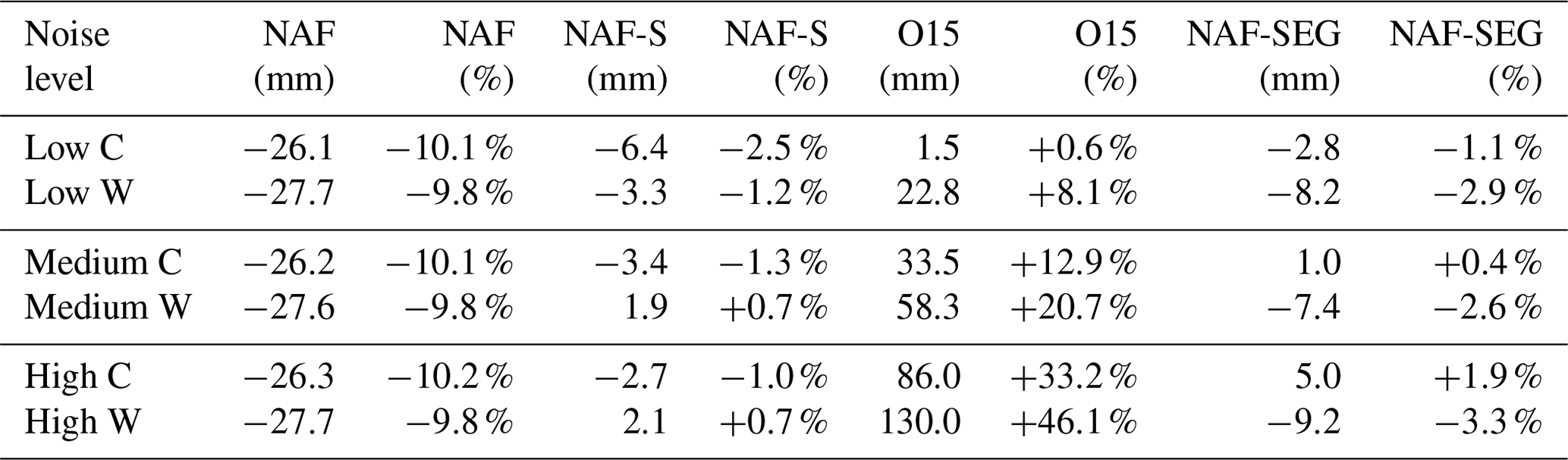
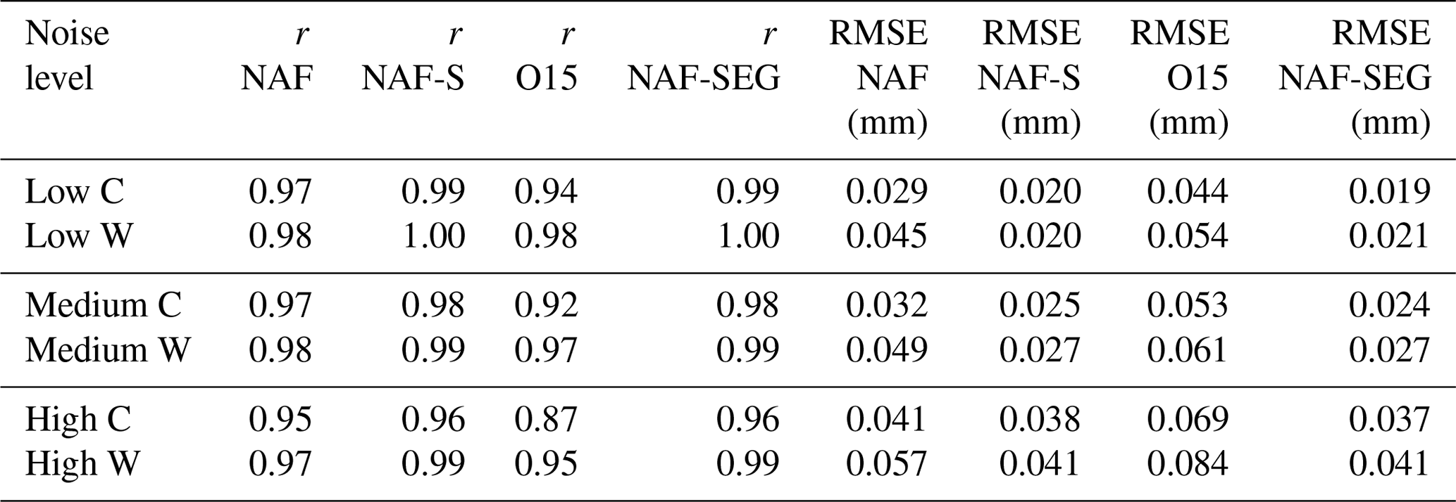
Table 3Correlation coefficient (r) and RMSE for NAF-SEG, NAF-S, NAF, and O15 post-processing techniques at different simulated noise levels for the cold (C) and warm (W) seasons.
4.1 Filter evaluation using pre-processed (control) data
The performance of the four filters was evaluated by adding synthetic noise and drift to clean (control) cold-season and warm-season time series and then assessing each filter's skill in recovering the control. The cold-season results are shown in Fig. 2, and an in-depth look at the first simulated cold-season evaporation event is shown in Fig. 3 for each of the three noise scenarios. The warm-season results (not shown) are very similar to the cold-season results in Figs. 2 and 3. Tables 2 to 4 show the associated 30 min total seasonal biases, correlation coefficients, and RMSE for all four filters as well as the NAF-SEG evaporation estimates, broken down by season.
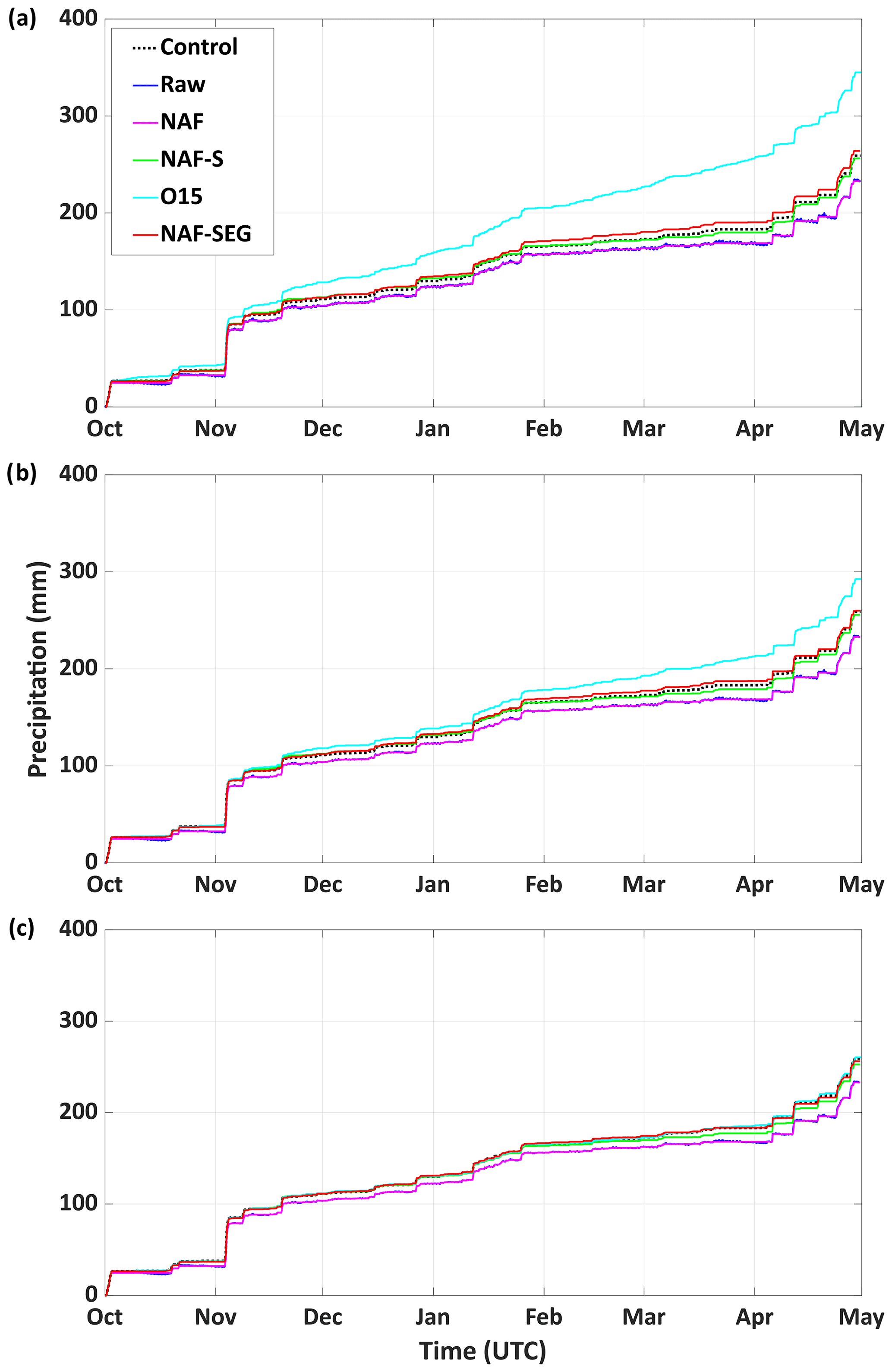
Figure 2Time series of simulated cold-season precipitation gauge bucket weight with synthetic evaporation and varying levels of synthetic noise and diurnal oscillations (a high noise; b medium noise; c low noise).
Based on their success in eliminating the added synthetic noise and drift and recovering the original control time series, NAF-S and NAF-SEG outperformed NAF and O15. O15 performed well at low noise but was sensitive to higher noise levels, with biases in total precipitation of +1 % (+8 %), +13 % (+21 %), and +33 % (+46 %) for the cold-season (warm-season) low-, medium-, and high-noise scenarios respectively. NAF was insensitive to noise but failed to recover the added evaporative losses (10 % of the precipitation total) at all noise levels. NAF-S and NAF-SEG performed well at all three noise levels, recovering the control precipitation to within 3 % of the total (regardless of season) and generating the highest correlation coefficients and lowest RMSE. NAF-SEG also produced an estimate of evaporation; its skill in detecting evaporative losses varied by both season and noise level. In the cold season, NAF-SEG overestimated the synthetic evaporation by 16 % at high noise and underestimated the synthetic evaporation by 19 % at low noise. In the warm season, NAF-SEG underestimated the synthetic evaporation by 10 % at high noise and 26 % at low noise. Given the inherent difficulty of deconvolving the evaporation and precipitation signals, and the high degree of temporal detail in the added evaporation time series, the ability of the NAF-SEG to detect and eliminate evaporative drift was encouraging. Indeed, the fully automated NAF-SEG was able to match the skill of the manually supervised NAF-S.
Table 4NAF-SEG evaporation estimates for different simulated noise levels, with actual evaporation constant at 25.9 mm in the cold-season (C) and 28.2 mm in the warm-season (W) control.
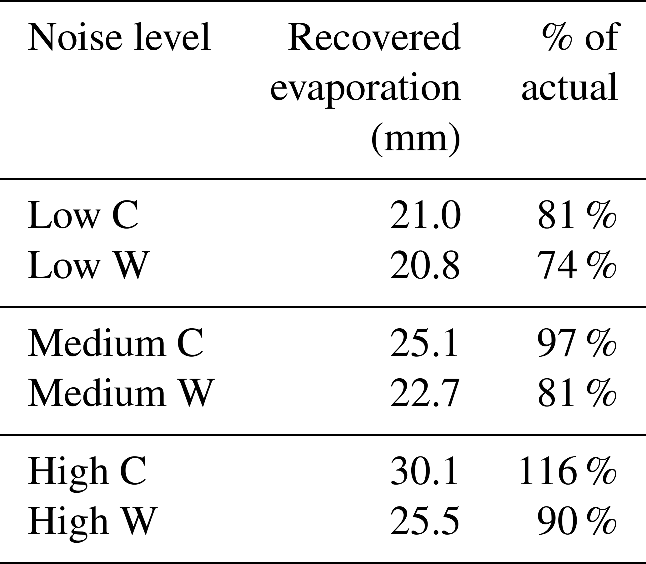
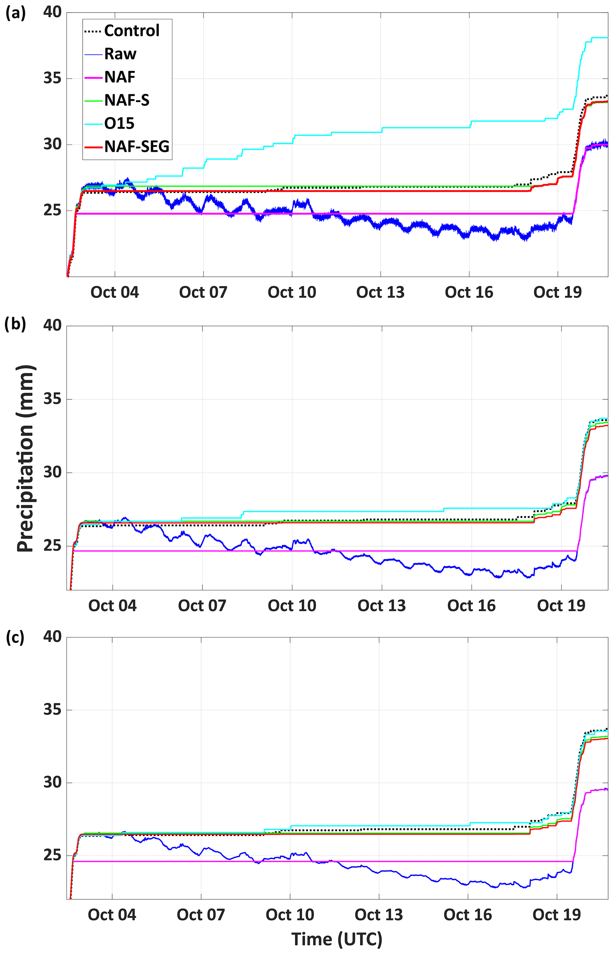
Figure 3Time series of simulated cold-season precipitation gauge bucket weight (zoomed into the first evaporation event) with synthetic evaporation and varying levels of synthetic noise and diurnal oscillations (a high noise; b medium noise; c low noise).
4.2 Filter evaluation using unprocessed data
This intercomparison examines the relative performance of the O15, NAF, and NAF-SEG on raw (minimally processed) weighing-gauge time series, using the NAF-S output as the reference standard. Individual results from the 44 cold-season and 11 warm-season test time series are shown in Tables A1 and A2 respectively. Overall, the NAF-SEG technique gave the lowest mean bias, highest mean correlation coefficient r, and lowest mean RMSD value (Table 5) in both seasons. In cold-season testing, the absolute bias from NAF-SEG was lower than the O15 bias in 37 of 44 cases (84 %), similar in 5 cases (11 %), and higher in 2 cases (5 %). In warm-season testing, NAF-SEG showed a lower or similar absolute bias in 7 of the 11 cases (64 %). NAF-SEG also produced the lowest variability in r, RMSD, and the seasonal total (Fig. 4; showing cold-season only), suggesting the greatest consistency in processing performance across sites, configurations, and years.
Table 5Mean correlation coefficients (r) and RMSD along with standard deviations (SDs) for all observed real-world precipitation time series using NAF-S as the reference (warm-season, May–September, in parenthesis).
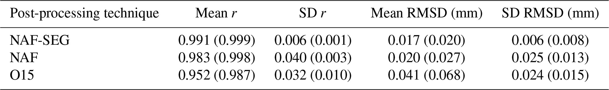
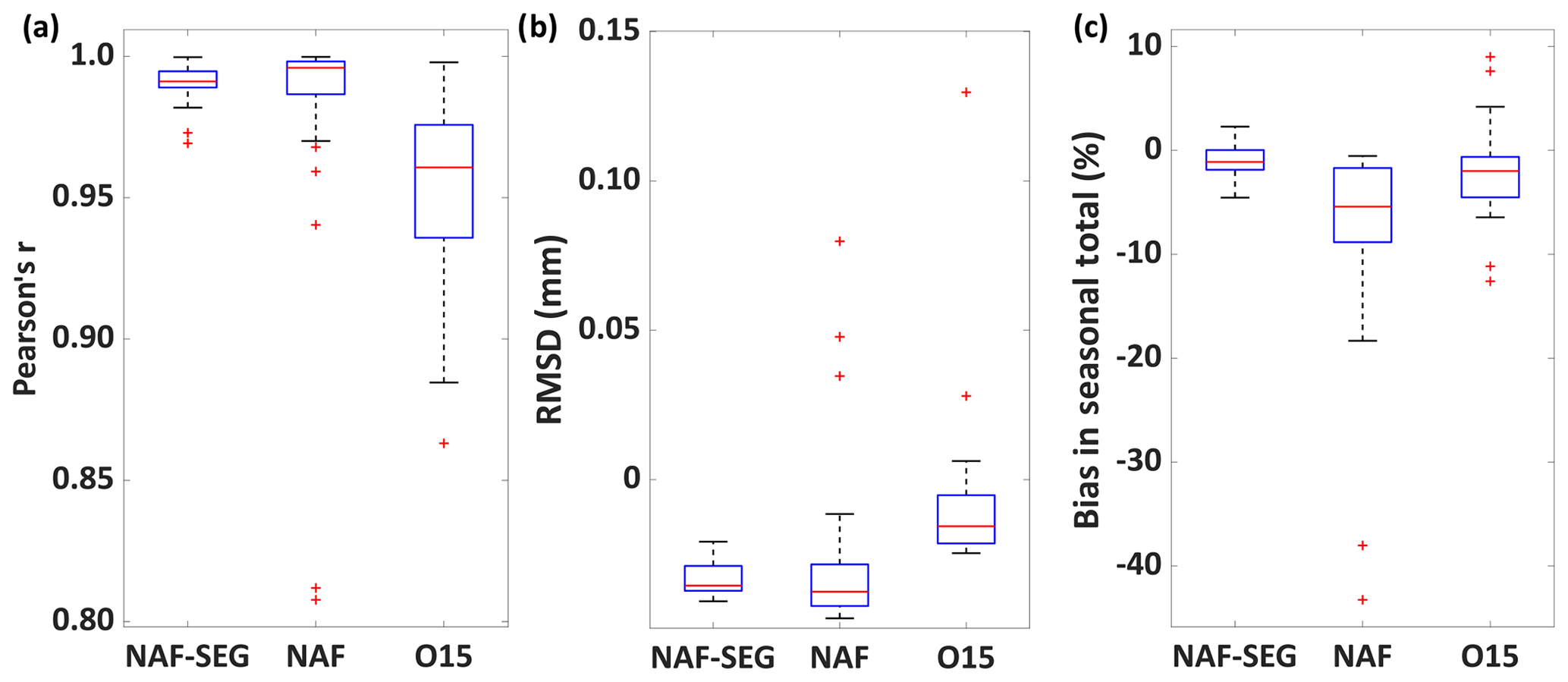
Figure 4Box-and-whisker plots of (a) Pearson's r, (b) RMSD, and (c) bias in cold-season total precipitation relative to the reference for each of the evaluated filtering techniques (NAF-SEG, NAF, and O15) as compared to the reference technique (NAF-S) for the 44 unprocessed time series.
The relative performance of NAF-SEG, NAF, and O15 varied across the 55 test time series, related to the nature and magnitude of the noise and negative drift due to evaporation from the bucket (Tables A1 and A2). Figure 5 shows four cold-season examples, comparing raw and processed time series. The y axis is scaled to the precipitation total to provide perspective on the relative errors in the processing techniques. The inset graphs in Fig. 5, which zoom in on particular events, highlight the magnitude of noise and drift in the raw data and show how the filters respond.
Figure 5a shows a time series for Caribou Creek (CCR), Canada, where the raw data exhibit very little noise or evaporation. For that reason, all processing techniques are within a few percent of the NAF-S reference, and it is difficult to see the differences during much of the time series. Figure 5b, from Haukeliseter (HKL), Norway, exhibits higher noise, resulting in an O15 precipitation overestimate of +9 % due to false precipitation detection. A moderate amount of evaporation is seen in the growing difference between NAF and NAF-S, with NAF-SEG nearly replicating NAF-S. Figure 5c and d, from Bratt's Lake (XBK), Canada, show cases with high evaporation (Fig. 5c) and high noise (Fig. 5d). In Fig. 5c, evaporation causes a low bias in NAF, which recovers only 87 % of the NAF-S precipitation total; O15 shows two compensating errors – an underestimation in precipitation due to evaporation and an increase in false precipitation detections due to noise, resulting in a recovery of 94 % of total precipitation relative to NAF-S, and NAF-SEG closely replicates NAF-S, with slight deviations in November and December. Figure 5d shows the impact of high noise with little evaporation; O15 overestimates precipitation by 4 %, whereas NAF-SEG is consistent with NAF-S throughout the time series.
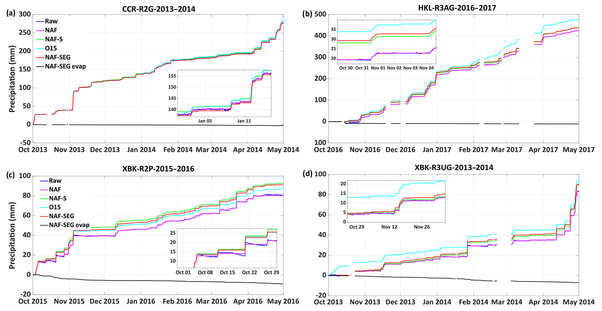
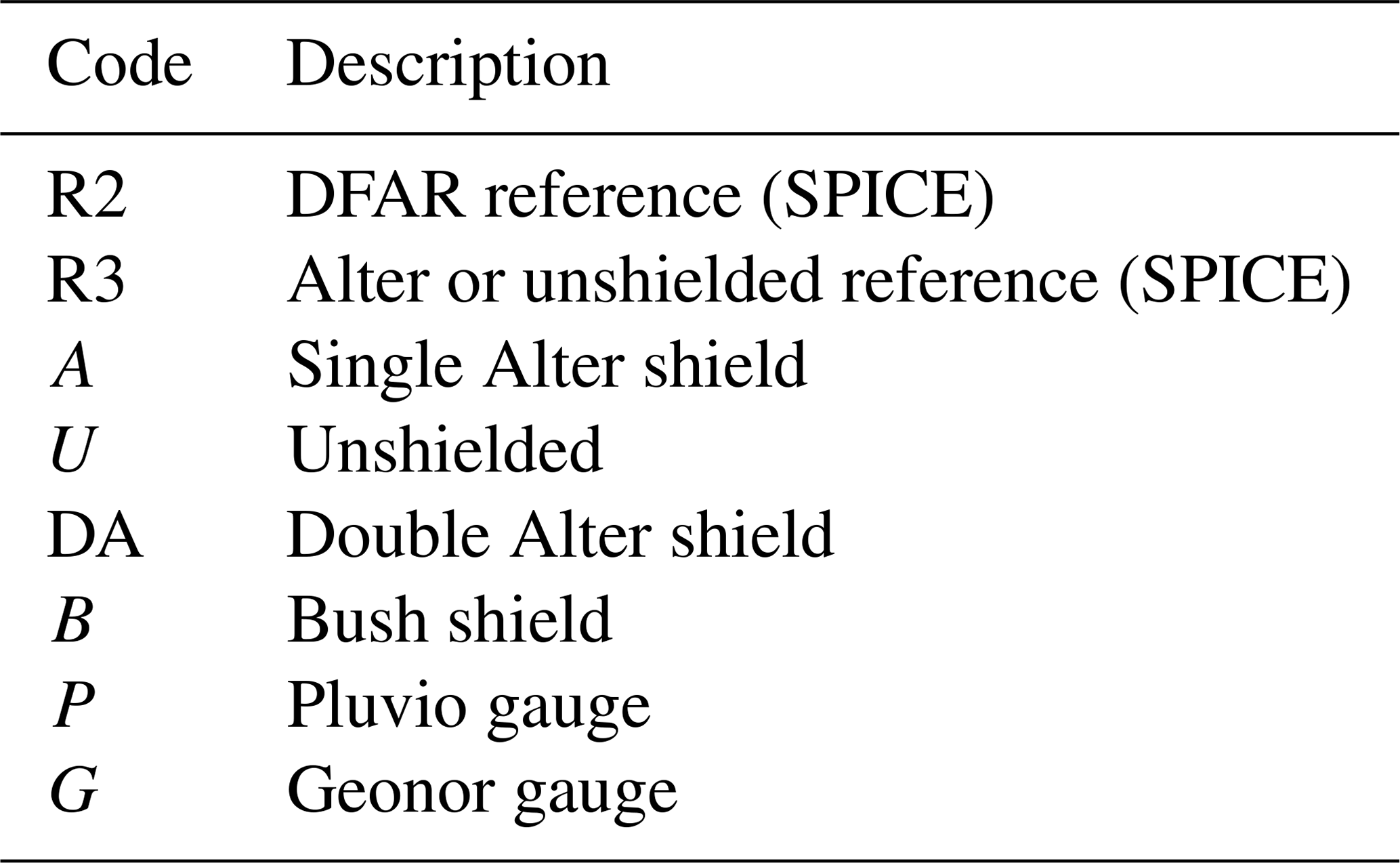
Figure 5Time series of observed cold-season precipitation gauge bucket-weight processing (NAF, NAF-S, O15, and NAF-SEG) along with the NAF-SEG evaporation estimate for (a) Caribou Creek R2G 2013–2014, (b) Haukeliseter R3AG 2016–2017, (c) Bratt's Lake R2P 2015–2016, and (d) Bratt's Lake R3UG 2013–2014. Insets show a zoomed example with consistent vertical scaling to illustrate the issues and filter performance relative to each time series.
This study evaluated four filters for processing the outputs of accumulating automated weighing precipitation gauges: three that were fully automated (O15, NAF, and NAF-SEG) and one that required manual supervision (NAF-S). Overall, NAF-S and NAF-SEG outperformed O15 and NAF; both NAF-S and NAF-SEG showed similar skill in compensating for evaporative losses and eliminating false detections caused by random noise and diurnal oscillations. O15 performed well in low-noise cases with minimal evaporation but generated false precipitation detections when the data were noisy and often underestimated evaporative losses. NAF performed well in cases with minimal evaporation regardless of the noise level but did not correct for evaporative losses. NAF-SEG performed consistently well and provided a fully automated alternative that matched the skill of the manual NAF-S method. Moreover, NAF-SEG added a direct estimate of evaporation, without the user intervention required by NAF-S or the 1 mm threshold required by O15. Similar evaporation estimates are not directly available from the other techniques.
Although NAF-SEG did not perfectly recover the synthetic evaporation that was added to the control time series (the recovery rates were 81 % to 116 % depending on the noise level), it performed as well as the manually supervised NAF-S technique. Both NAF-S and NAF-SEG failed to disentangle precipitation and evaporation when they occurred on the same day. The challenge to do so may be insurmountable. The imperfect recovery of synthetic evaporation, coupled with the sensitivity of the recovered evaporation to noise, highlights the need to implement measurement protocols that minimize evaporative losses. We recommend the use of NAF-SEG as a screening technique to identify gauges and locations that have significant evaporative losses and then to implement adequate measures to minimize those losses, such as modifications to the oil and antifreeze mixture used to prevent freezing and evaporation.
Overestimation of precipitation by the O15 method occurs when the noise exceeds the filter's prescribed threshold of 0.2 mm. This value for the threshold has been set based on experience as a necessary and calculated balance between eliminating real precipitation events and detecting false events. When the noise level is low, as in the low-noise scenario of the control data, the O15 technique works successfully. However, noise patterns vary substantially from site to site and among gauges, as illustrated by Nitu et al. (2018), and often exceed the filtering capabilities of O15. It should also be noted that the unprocessed data in our tests were pre-filtered using a Gaussian filter with a 4 min window, which was integrated into the SPICE quality control process prior to testing the algorithms. This likely resulted in the O15 performing better than it would have in the operational setting, but this was not confirmed.
The NAF technique is fundamentally effective at filtering noise and diurnal oscillations but underestimates precipitation when evaporative losses occur because the algorithm forces the precipitation total to match the final raw bucket weight in the time series, with evaporation assumed to be zero. The NAF-SEG technique, which implements NAF over 24 h windows, maintains all the strengths of NAF with the added functionality of automating the detection and removal of bucket evaporation. Neither NAF-S nor NAF-SEG removes evaporation perfectly, particularly when it occurs in combination with precipitation, but both represent a major step forward compared to other processing methods. We attribute the effectiveness of NAF-SEG to two characteristics of precipitation events: first that evaporation is relatively small during periods with precipitation and second that both precipitation and evaporation are persistent over timescales of days. In the development of NAF-SEG, a 24 h moving window was chosen to minimize the impact of temperature-related diurnal oscillations, but fortuitously the 24 h window also served to separate days with precipitation and little evaporation from days with evaporation and little or no precipitation. The performance of NAF-SEG may decline when signal noise is due to non-cyclical temperature fluctuations, such as those that occur during strong synoptic events. Although this possibility was not assessed, it is one that users should be aware of.
As mentioned in the introduction to NAF-SEG, a sensitivity analysis was performed for a range of P* values from 0.0001 to 0.5 mm using the pre-processed high-noise time series for both warm and cold seasons. The analysis showed negligible sensitivity as P* ranged from 0.0001 to 0.05 and higher sensitivity as P* further increased to 0.5 mm for both seasons. Given the relative insensitivity of NAF-SEG to P* < 0.5 mm, the use of 0.001 mm seems to be an appropriate baseline value for both seasons; users may want to further experiment with the parameter as their own data require.
NAF-SEG provides an attractive alternative to NAF when negative evaporative drift is present in the raw data, but it is not designed to handle all contingencies. For instance, unexplained positive then negative excursions in bucket weight are sometimes observed. If the positive and negative excursions are separated by more than 24 h (the size of the window), the NAF-SEG will errantly attribute the positive excursion to precipitation and the negative excursion to evaporation.
The results of the testing on unprocessed time series from different sites, seasons, and gauge configurations showed that NAF-SEG generally outperformed O15 in both cold- and warm-season test cases. Of the 44 cold-season test cases, O15 outperformed NAF-SEG in only two cases: the DFAR and unshielded Pluvio2 gauges at WFJ (2016–2017). However, these gauges may not have been serviced adequately; note the extreme evaporation rates as evidenced in the high biases between NAF and NAF-S in Table A1. This diminishes their usefulness for this evaluation; they were among the most challenging to process, with the greatest uncertainty in the supervised NAF-S output that served as the reference standard.
Filter evaluation was more limited in the warm season because the raw site data were obtained from the SPICE project, which focused on the measurement of solid precipitation. Still, we were able to assemble 11 warm-season cases. The warm-season data were expected to differ from the cold-season data in two respects: higher evaporative losses and different noise characteristics. Each of the filters generated a higher RMSD in the warm season than the cold season; the greatest increase was found for O15, consistent with the pre-processed control experiments. In general, NAF-SEG outperformed both NAF and O15 in the warm season. NAF-SEG outperformed O15 in all warm season cases for r and RMSD and resulted in a lower or similar seasonal bias in 7 of the 11 cases. The NAF-SEG totals consistently underestimated warm-season precipitation, but the biases were small, averaging 1.7 % compared with 1.0 % for the cold season. Regardless of the sample size, the performance metrics all show that NAF-SEG outperformed both NAF and O15 in the warm season as well as the cold season.
The evaluation of filter performance based on raw site data begs the following question: how reliable are the NAF-S outputs as reference standards, given that they rely on the operator's subjective judgement during the interactive elimination of negative drift and other spurious bucket-weight changes? We acknowledge that operator bias is possible but are confident that its impact in this study is minimal. A single, skilled operator processed all of the data and made every attempt to apply the NAF-S method consistently. Adding further confidence to the NAF-S outputs are the tests with control data, which independently demonstrated the efficacy of the NAF-S to eliminate noise and evaporative drift.
One suggestion to improve the quality of data from accumulating precipitation gauges is to add disdrometers, which detect the current weather conditions, to the site measurements and then incorporate their outputs into the quality control and filtering process. These augmented observations could be used to refine the noise filtering by automating the high-temporal-resolution (e.g. 1 min) detection of light precipitation events and assist in removing false precipitation detections. These ancillary data were used in this way during SPICE (Nitu et al., 2018) and should be further explored for enhancing operational filtering.
This study reports the development and implementation of a robust, fully automated technique for post-processing data from automated weighing precipitation gauges. The NAF-SEG technique is designed to eliminate varying levels of random noise and diurnal oscillations as well as correcting for negative drift from bucket evaporation. An intercomparison of four filtering techniques shows that the O15, although simple and deployable in real time, fails when noise levels exceed the filter's threshold and may undercompensate for bucket evaporation. NAF, although highly effective in eliminating noise, does not correct for evaporative losses. NAF-S, which adds manual supervision to NAF, is effective in removing noise, eliminating spurious data, and correcting for negative drift from evaporation. However, it is labour-intensive and best suited to complete seasonal time series.
Our results show that NAF-SEG is equally as effective as NAF-S in eliminating noise and evaporative drift from automated weighing-gauge precipitation measurements. When tested against a control data set with added synthetic noise and evaporation, NAF-SEG was able to recover the original control to within ±3 % of the total, with a lower RMSE than the other techniques. When evaluated on 55 raw time series from various sites, years, and gauge configurations, NAF-SEG outperformed O15 and NAF and gave the highest mean correlation coefficient and lowest mean RMSD.
One limitation of NAF-SEG is that it requires 24 h data segments; consequently, it cannot be deployed for real-time processing of automated weighing-gauge precipitation measurements. Until other alternatives are found, we recommend the use of a simple threshold filter like O15 for real-time applications, but with the archiving of the raw 1 min time series for subsequent enhanced quality control, reprocessing using NAF-SEG, and the archiving of the NAF-SEG outputs. This, in combination with routine site servicing to minimize evaporation and other sources of noise, can result in improved operational precipitation data.
Table A1Cold-season total precipitation (unfiltered, NAF-S, and NAF-SEG filtered), filter biases (NAF, O15, and NAF-SEG), and derived bucket evaporation (NAF-SEG) from 44 WMO SPICE precipitation time series. Biases (mm) are calculated using NAF-S as the reference filtering technique. Filtered time series that do not show an improvement with the NAF-SEG method when compared to O15 are indicated by an asterisk (*).
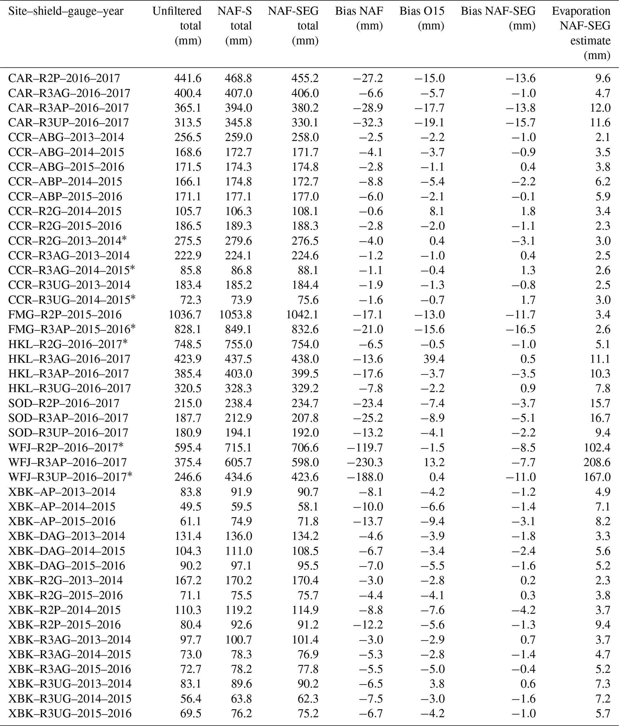
Table A2Warm-season total precipitation (unfiltered, NAF-S, and NAF-SEG filtered), filter biases (NAF, O15, and NAF-SEG), and derived bucket evaporation (NAF-SEG) from 11 WMO SPICE precipitation time series. Biases (mm) are calculated using NAF-S as the reference filtering technique. Filtered time series that do not show an improvement with the NAF-SEG method when compared to O15 are indicated by an asterisk (*).
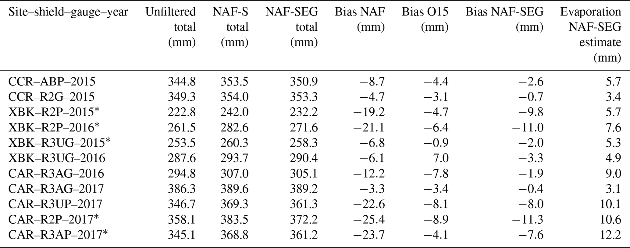
Table A3A description of the different shield and gauge configurations used in Tables A1 and A2.
The code for NAF-SEG and the precipitation time series intercomparison data used in this evaluation are available at https://doi.org/10.20383/101.0243 (Ross et al., 2020).
AR is the lead author and was responsible for the processing and analysis of these data. AR also completed much of the coding required to implement the data processing. CDS oversaw the development of this project and provided guidance in the analysis and the development of this paper. AB designed and coded the NAFs and provided guidance in the analysis and in the writing of this paper.
The authors declare that they have no conflict of interest.
The authors would like to thank Daqing Yang of Environment and Climate Change Canada (Victoria) for providing an internal review of this paper. We would like to acknowledge the organizations that collected and provided the observed data from the WMO SPICE sites for this analysis: Environment and Climate Change Canada (Climate Research Division and the Meteorological Service of Canada Observing Systems and Engineering), the Norwegian Meteorological Institute, MeteoSwiss, the Finnish Meteorological Institute, and the Spanish State Meteorological Agency. Lastly, we would like to express our appreciation to the anonymous referees, who helped to improve this paper with their insightful questions and suggestions.
This paper was edited by Daqing Yang and reviewed by two anonymous referees.
Barnett, T. P., Adam, J. C., and Lettenmaier, D. P.: Potential impacts of a warming climate on water availability in snow dominated regions, Nature, 438, 303–309, 2005.
Bartlett, P. A., MacKay, M. D., and Verseghy, D. L.: Modified snow algorithms in the Canadian Land Surface Scheme: Model runs and sensitivity analysis at three boreal forest stands, Atmos. Ocean, 44, 207–222, 2006.
Bush, E. and Lemmen, D. S. (Eds.:) Canada's Changing Climate Report, Government of Canada, Ottawa, ON, 444 pp., 2019, available at: https://changingclimate.ca/CCCR2019/, last access: 9 April 2019.
Duchon, C. E.: Using vibrating-wire technology for precipitation measurements, in: Precipitation: Advances in Measurement, Estimation and Prediction, editied by: Michaelides, S., Springer, Berlin, Heidelberg, 33–58, https://doi.org/10.1007/978-3-540-77655-0_2, 2008.
Geonor: T-200B series precipitation gauge manual for 600-mm, 1000-mm & 1500-mm capacity gauges, available at: http://geonor.com/live/wp-content/uploads/2014/10/T-200B-US-Manual.-rev-10.10-20150128.pdf, last access: 9 April 2019.
Goodison, B., Louie, P., and Yang, D.: The WMO solid precipitation measurement intercomparison, World Meteorological Organization-Publications-WMO/TD No. 872, 212 pp., 1998.
Goodison, B. E.: Accuracy of Canadian snow gauge measurements, J. Appl. Meteorol., 17, 1542–1548, 1978.
Harder, P. and Pomeroy, J.: Estimating precipitation phase using a psychrometric energy balance method, Hydrol. Process., 27, 1901–1914, https://doi.org/10.1002/hyp.9799, 2013.
Kochendorfer, J., Rasmussen, R., Wolff, M., Baker, B., Hall, M. E., Meyers, T., Landolt, S., Jachcik, A., Isaksen, K., Brækkan, R., and Leeper, R.: The quantification and correction of wind-induced precipitation measurement errors, Hydrol. Earth Syst. Sci., 21, 1973–1989, https://doi.org/10.5194/hess-21-1973-2017, 2017a.
Kochendorfer, J., Nitu, R., Wolff, M., Mekis, E., Rasmussen, R., Baker, B., Earle, M. E., Reverdin, A., Wong, K., Smith, C. D., Yang, D., Roulet, Y.-A., Buisan, S., Laine, T., Lee, G., Aceituno, J. L. C., Alastrué, J., Isaksen, K., Meyers, T., Brækkan, R., Landolt, S., Jachcik, A., and Poikonen, A.: Analysis of single-Alter-shielded and unshielded measurements of mixed and solid precipitation from WMO-SPICE, Hydrol. Earth Syst. Sci., 21, 3525–3542, https://doi.org/10.5194/hess-21-3525-2017, 2017b.
Leeper, R. D., Palecki, M. A., and Davis, E.: Methods to Calculate Precipitation from Weighing-Bucket Gauges with Redundant Depth Measurements, J. Atmos. Ocean. Tech., 32, 1179–1190, https://doi.org/10.1175/JTECH-D-14-00185.1, 2015.
Mekis, E., Donaldson, N., Reid, J., Zucconi, A., Hoover, J., Li, Q., Nitu, R., and Melo, S.: An Overview of Surface-Based Precipitation Observations at Environment and Climate Change Canada, Atmos. Ocean, 56, 71–95, https://doi.org/10.1080/07055900.2018.1433627, 2018.
Nemeth, K.: OTT Pluvio2: Weighing precipitation gauge and advances in precipitation measurement technology, TECO-2008 – WMO Technical Conference on Meteorological and Environmental Instruments and Methods of Observation (TECO-2008), Russian Federation, St. Petersburg, 27–29 November 2008.
Nitu, R., Roulet, Y.-A., Wolff, M., Earle, M., Reverdin, A., Smith, C., Kochendorfer, J., Morin, S., Rasmussen, R., Wong, K., Alastrué, J., Arnold, L., Baker, B., Buisán, S., Collado, J. L., Colli, M., Collins, B., Gaydos, A., Hannula, H.-R., Hoover, J., Joe, P., Kontu, A., Laine, T., Lanza, L., Lanzinger, E., Lee, G. W., Lejeune, Y., Leppänen, L., Mekis, E., Panel, J.-M., Poikonen, A., Ryu, S., Sabatini, F., Theriault, J., Yang, D., Genthon, C., van den Heuvel, F., Hirasawa, N., Konishi, H., Motoyoshi, H., Nakai, S., Nishimura, K., Senese, A., and Yamashita, K.: WMO Solid Precipitation Intercomparison Experiment (SPICE) (2012–2015), World Meteorological Organization Instruments and Observing Methods Report No. 131, Geneva, available at: http://www.wmo.int/pages/prog/www/IMOP/publications-IOM-series.html (last access: 28 May 2020), 2018.
Pan, X., Yang, D., Li, Y., Barr, A., Helgason, W., Hayashi, M., Marsh, P., Pomeroy, J., and Janowicz, R. J.: Bias corrections of precipitation measurements across experimental sites in different ecoclimatic regions of western Canada, The Cryosphere, 10, 2347–2360, https://doi.org/10.5194/tc-10-2347-2016, 2016.
Peters, A., Nehls, T., Schonsky, H., and Wessolek, G.: Separating precipitation and evapotranspiration from noise – a new filter routine for high-resolution lysimeter data, Hydrol. Earth Syst. Sci., 18, 1189–1198, https://doi.org/10.5194/hess-18-1189-2014, 2014.
Rasmussen, R., Baker, B., Kochendorfer, J., Meyers, T., Landolt, S., Fischer, A. P., Black, J., Thériault, J. M., Kucera, P., Gochis, D., Smith, C., Nitu, R., Hall, M., Ikeda, K., and Gutmann, E.: How well are we measuring snow: The noaa/faa/ncar winter precipitation test bed, B. Am. Meteorol. Soc., 93, 811–829, https://doi.org/10.1175/BAMS-D-11-00052.1, 2012.
Ross, A. D., Smith, C. D., and Barr, A. G.: Precipitation gauge time series used in evaluating post-processing filters (code included), FRDR, https://doi.org/10.20383/101.0243, 2020.
Sevruk, B. and Chvíla, B.: Error sources of precipitation measurements using electronic weight systems, Atmos. Res., 77, 39–47, https://doi.org/10.1016/j.atmosres.2004.10.026, 2005.
Sevruk, B., Hertig, J.-A., and Spiess, R.: The effect of a precipitation gauge orifice rim on the wind field deformation as investigated in a wind tunnel, Atmos. Environ. A-Gen., 25, 1173–1179, 1991.
Sevruk, B., Ondras, M., and Chvila, B.: The WMO precipitation measurement intercomparisons, Atmos. Res., 92, 376–380, 2009.
Smith, C. D.: The relationship between snowfall catch efficiency and wind speed for the Geonor T-200B precipitation gauge utilizing various wind shield configurations, Canmore, Alberta, 20–23 April 2009, 115–121, 2009.
Smith, C. D., Yang, D., Ross, A., and Barr, A.: The Environment and Climate Change Canada solid precipitation intercomparison data from Bratt's Lake and Caribou Creek, Saskatchewan, Earth Syst. Sci. Data, 11, 1337–1347, https://doi.org/10.5194/essd-11-1337-2019, 2019.
Wolff, M. A., Isaksen, K., Petersen-Øverleir, A., Ødemark, K., Reitan, T., and Brækkan, R.: Derivation of a new continuous adjustment function for correcting wind-induced loss of solid precipitation: results of a Norwegian field study, Hydrol. Earth Syst. Sci., 19, 951–967, https://doi.org/10.5194/hess-19-951-2015, 2015.
Yang, D., Kane, D., Zhang, Z., Legates, D., and Goodison, B.: Bias-corrections of long-term (1973–2004) daily precipitation data over the northern regions, Geophys. Res. Lett., 32, L19501, https://doi.org/10.1029/2005GL024057, 2005.
- Abstract
- Introduction
- Processing techniques under test
- Filter evaluation
- Results
- Discussion
- Conclusions
- Appendix A: Raw time series used in precipitation filter evaluation, with evaporation estimates and total precipitation bias
- Code and data availability
- Author contributions
- Competing interests
- Acknowledgements
- Review statement
- References