First observations of the McMurdo–South Pole oblique ionospheric HF channel

We present the first observations from a new low-cost oblique ionosonde located in Antarctica. The transmitter is located at McMurdo Station, Ross Island, and the receiver at Amundsen–Scott Station, South Pole. The system was demonstrated successfully in March 2019, with the experiment yielding over 30 000 ionospheric echoes over a 2-week period. These data indicate the presence of a stable E layer and a sporadic and variable F layer with dramatic spread F of sometimes more than 500 km (in units of virtual height). The most important ionospheric parameter, NmF2, validates well against the Jang Bogo Vertical Incidence Pulsed Ionospheric (VIPIR) ionosonde (observing more than 1000 km away). GPS-derived TEC data from the Multi-Instrument Data Analysis Software (MIDAS) algorithm can be considered necessary but insufficient to predict 7.2 MHz propagation between McMurdo and the South Pole, yielding a true positive in 40 % of cases and a true negative in 73 % of cases. The success of this pilot experiment at a total grant cost of USD 116 000 and an equipment cost of ∼ USD 15 000 indicates that a large multi-static network could be built to provide unprecedented observational coverage of the Antarctic ionosphere.

1 Introduction

1.1 High-latitude ionospheric variability

The high-latitude ionosphere frequently exhibits dramatic variability. Some of the first observations of these phenomena were made by Meek (1949) using an HF sounder at Baker Lake, Canada. Using an unprecedented and currently unmatched network of ionosondes, Hill (1963) gave the first clear picture of the phenomenon we have come to understand as the tongue of ionization (e.g., Foster, 1989) and showed it breaking into a patch. This F-layer ionospheric variability is caused primarily by dense, photo-ionized plasma being convected into the polar caps (e.g., Lockwood and Carlson, 1992). Most theories explaining this behavior are skewed heavily towards the Northern Hemisphere due to better observational coverage there. Investigations covering the Southern Hemisphere continue to produce apparently contradictory results. For example, Noja et al. (2013), Xiong et al. (2018), and Chartier et al. (2019) find more variability around December or January, whereas Coley and Heelis (1998), Spicher et al. (2017), and David et al. (2019) show a maximum in June or July. One thing these authors agree on is that the Antarctic ionosphere is far more variable than the Arctic and up to twice as variable during summer. New observations are needed in the southern polar cap to resolve this controversy. The F-layer peak density (called NmF2) must be observed separately from the E layer, whose peak density (called NmE) can be equivalent or even greater than NmF2 at high latitudes (e.g., Hatton, 1961). The horizontal extent of these features can be hundreds or thousands of kilometers, so a relatively low-cost approach is required that can provide spatially distributed observations. High temporal cadence is also essential, given that horizontal drift velocities of 5000 km h⁻¹ (approximately 1400 m s⁻¹) have been reported by Hill (1963). Another area of current scientific interest is E–F coupling, where forcing applied to the E layer through neutral dynamics or other drivers appears to map into the F layer (e.g., Cosgrove and Tsunoda, 2004; Saito et al., 2007). This phenomenon is perhaps easiest to observe at high magnetic latitudes, where the dip angle is almost vertical and so any E–F coupling should be spatially localized, rather than being separated by hundreds or thousands of kilometers as is the case at middle or low latitudes. In general, the Antarctic ionosphere is of great scientific interest because it provides potentially the best ground base from which to observe deep polar cap dynamics, which may reveal new insights into direct coupling between the Solar wind and Earth's atmosphere. This is because magnetic field lines at very high latitudes are typically “open” rather than closing in the magnetosphere.

1.2 Ionospheric remote sensing using radio signals

Radio signal propagation has been integrally linked with ionospheric research since Marconi's famous transatlantic experiment in 1901. The first ionosonde was built by Breit and Tuve (1925). The instrument works by transmitting radio signals of increasing frequency and then receiving their ionospheric echoes. The time of flight between transmission and reception is used to estimate their virtual range (by assuming that the signals traveled at the speed of light in free space). The maximum observed frequency (MOF) is the highest-frequency signal that is received on the ground. If sufficiently close frequency spacing is used for the transmissions and if the signal's angle of incidence with the ionosphere (θ) is known, MOF can be related to the critical frequency of the ionosphere (foF2) by Eq. (1):

$$\begin{array}{}\text{(1)}& \text{foF2}\approx \text{MOF}\cdot \cos \mathit{\theta }.\end{array}$$

Once obtained, foF2 (in hertz) is easily converted to NmF2 (in electrons per cubic meter) via Eq. (2):

$$\begin{array}{}\text{(2)}& \text{NmF2}\approx {\left({\displaystyle \frac{\text{foF2}}{\mathrm{9}}}\right)}^{\mathrm{2}}.\end{array}$$

The same approach can be employed for echoes returned below the peak height, so that bottom side electron density profiles can be retrieved from vertical or oblique ionosondes. It is important to note that the formulation in Eqs. (1) and (2) is based only on ordinary-mode wave propagation and that mode splitting can occur in the presence of transverse magnetic fields, further adding to the uncertainty of NmF2 retrievals. Budden (1961) provides a comprehensive description of radio wave propagation in the ionosphere.

Although their numbers have reduced since the International Geophysical Year (1957–1958), substantial networks of ionosondes exist today, notably the Digisonde network of about 50 instruments (Reinisch et al., 2018), the Canadian High Arctic Ionosonde Network of about 7 instruments, and several installations of the sophisticated Vertical Incidence Pulsed Ionospheric Radar (VIPIR) system (Bullett et al., 2016). However, coverage is very sparse in the southern polar cap, with only the VIPIR at Jang Bogo producing reliable, high (2 min) temporal cadence observations.

Oblique sounding has some advantages compared to vertical-mode operation for ionospheric sounding. Principal among these is the ability to observe a location (or locations) in the ionosphere spatially separated from the ground infrastructure. This is important when operating in remote areas such as Antarctica, where the cost of installing and maintaining ground stations is high. Of course, this benefit comes with an associated challenge in interpreting the data, as the signal path through the ionosphere is unknown. Oblique sensing also provides for potentially large networks of observations to be built using a relatively small number of transmitters. That is important because HF transmitters require far more power and larger antennas than receivers and also often create broadcast licensing issues. Therefore, oblique sounding may be useful in expanding the spatial coverage of ionospheric observations, especially in remote areas.

1.3 Low-cost, open-source ionospheric remote sensing

The number of ionosondes in existence and the availability of their data are restricted by their typically high cost and proprietary status. Recent developments in meteor radar observation provide a means of solving this problem. Vierinen et al. (2016) observed meteor echoes in Germany using coded continuous wave transmissions at a fixed frequency, using a software-defined radio system. In communications terms, this is analogous to direct-sequence spread-spectrum modulation. The coded continuous wave approach provides substantial signal processing gain and allows for reduced peak transmitted power compared to a pulsed system. It also reduces false positive detections and allows for a multi-static network of transmitters and receivers to be developed. Signals from different transmitters can be separated through post-processing because each one uses a different pseudo-random code on the same frequency (Vierinen et al., 2016). Although the technique requires modification for ionospheric remote sensing, its availability through MIT Haystack's DigitalRF software-defined radio package (Volz et al., 2019) is a major advantage to this investigation. A separate open-source ionospheric sounder (also based on a meteor radar technique) has recently been developed by Bostan et al. (2019) and is available as part of the GnuRadar package.

2 Method

2.1 Coded continuous wave ionosonde

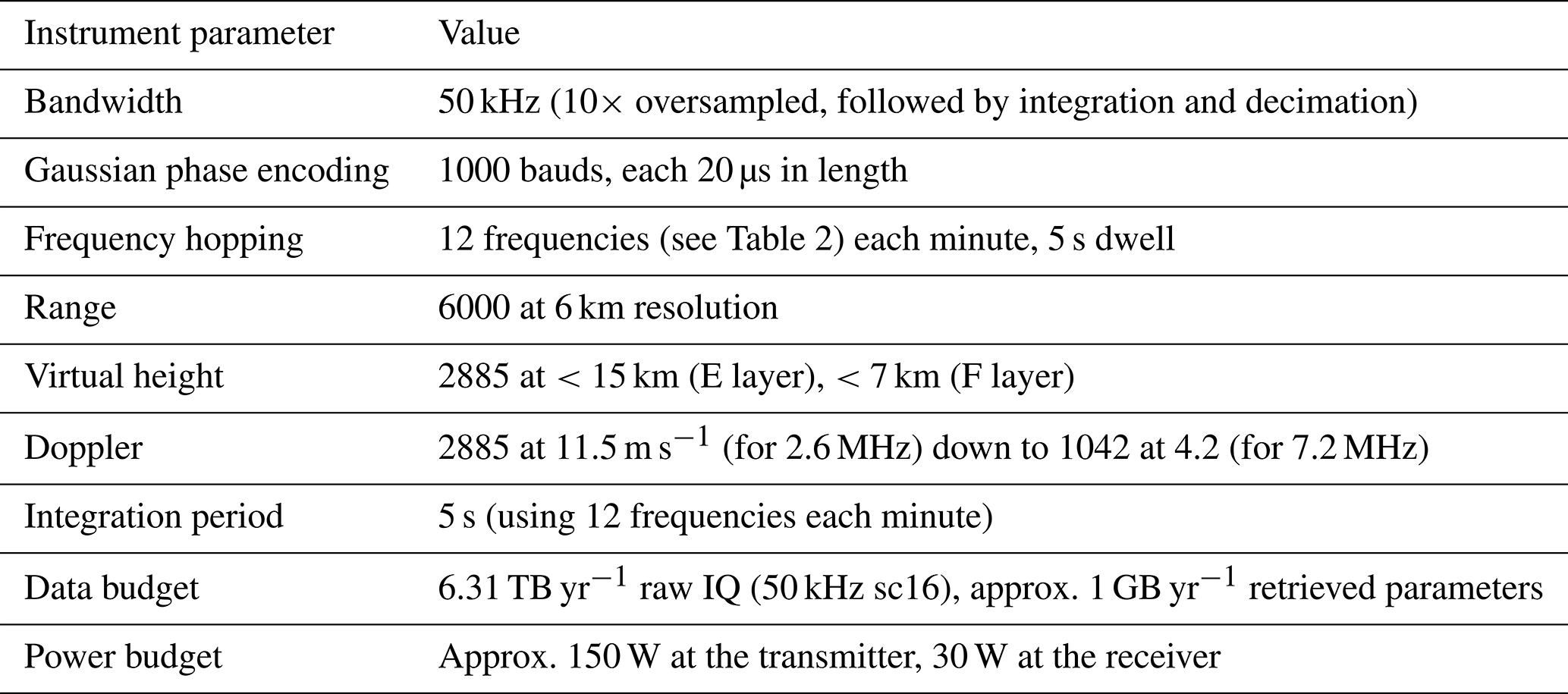
We modify the Vierinen et al. (2016) meteor radar approach for ionospheric sounding by adding a frequency-hopping capability. This new code makes the transmitter and receiver step through a pre-defined list of frequencies at specified seconds past each minute. GPS timing signals trigger the oscillators to retune at precisely the same time at both stations. In the present application, this retuning occurs every 5 s, allowing the system to cover 12 frequencies each minute, but up to 60 frequencies could be used without modification of the underlying software – the smaller number of frequencies allows for longer integration time and therefore increases sensitivity. Frequencies were selected based on International Reference Ionosphere (IRI) ray tracing (with a larger extent selected than was indicated by the ray tracing) and to remain >250 kHz away from any Antarctic HF communications channel. We coordinated with McMurdo communications to test for any interference with their operations and found no effect on their system. However, in principle the hardware supports operation anywhere in the HF band, while the software could operate at any frequency, and the operating schedule can be changed simply by editing text files in the transmitter and receiver computers. Aside from that modification, the system is essentially unchanged from that used by Vierinen et al. (2016). The transmitter and receiver bandwidth is effectively 50 kHz (with 10 times oversampling followed by integration and decimation employed at the receiver to reduce noise). The code consists of pseudo-random binary phase modulations of 1000 bauds in length, each 20 µs duration, yielding 6000 km un-aliased range resolution. Table 1 provides a summary of the instrument characteristics as configured for this experiment.

Table 1 Instrument characteristics.

The following data processing is applied to the received 50 kHz baseband signal centered on each frequency. Signals have DC offsets removed, have non-Gaussian components rejected to mitigate radio-frequency interference, and are then autocorrelated with the pseudo-random code to produce range–Doppler–intensity matrices for each 5 s analysis period. All signals >6 dB above the noise floor of the receiver are sent back as sparse range–Doppler–intensity matrices whenever internet access is available, while the raw in-phase and quadrature samples are stored on-site in DigitalRF format for future retrieval and analysis. The result is a remotely controllable instrument that has a data budget of only a few megabytes per day and delivers ionospheric soundings at a cadence of 1 min. The code for this system is publicly available at https://github.com/alexchartier/sounder (last access: 27 May 2020).

2.2 Installation in Antarctica

Having received a grant of USD 116 000 from the National Science Foundation's Office for Polar Programs, we developed, built, tested, and deployed the system in Antarctica. The total equipment cost for this experiment was approximately USD 15 000. The system's configuration is shown in Fig. (1). The transmitter is located at McMurdo Station, on the southern exposure of Observation Hill on the former site of the nuclear power station, with the electronics housed in a galvanized steel cabinet assembled by the principal investigator. The receiver is at South Pole Station, with the electronics housed in the V8 Vault (also home to VLF electronics used by LaBelle et al., 2015), currently located around 10 m under the ice ∼1 km from the main base. This configuration provides for oblique sounding of the ionosphere approximately halfway between McMurdo and the South Pole. Both sites have internet connection (typically 8 out of 24 h at South Pole) so observations are typically returned to Lab servers for analysis within a day of being taken. At various stages during testing, the system was remotely reconfigured through secure shell connection (SSH) to use different frequencies and output power levels.

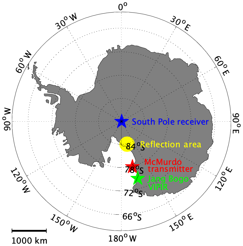
Figure 1 Experimental configuration with transmitter at McMurdo (red), receiver at South Pole (blue), approximate ionospheric reflection area (for single hop propagation) at midpoint between them (yellow), and validation instrument (VIPIR) at Jang Bogo station (green).

2.2.1 Transmitter

The transmit antenna is a broadband 50 m Barker and Williamson tilted, terminated folded dipole costing around USD 2000 and mounted in an east–west inverted-vee configuration on a 15 m central mast and 5 m stub masts. The transmitter electronics are made up of an Ettus Research USRP N210 with GPS-disciplined oscillator and BasicTx daughter board (National Instruments, 2020). The final-stage amplifier is a Motorola-designed AN762-180 (Granberg, 1980). Based on the power∕standing-wave ratio (SWR) meter installed on-site, we estimate that the system produced <50 W total transmitted power. Over the course of the experiment, the amplifier developed distortion leading to excessive SWR and out-of-band emissions, so it is not recommended for future installations.

2.2.2 Receiver

At the receiver site, an inexpensive 1 m active broadband dipole antenna is mounted around 2 m above the ice and connected to the receiver by 183 m of RG-6 cable. The antenna receives phantom power from a bias tee located in the vault. Inside the vault, the signal is boosted ∼20 dB by a low-noise amplifier and connected to a USRP N210 with BasicRx daughter board and GPS-disciplined oscillator. The receiver's oscillator retunes according to the pre-defined frequency schedule based on a timed command triggered by the GPS pulse-per-second signal.

2.3 Data processing

Ionospheric products are estimated by selecting the shortest range returns at the highest frequencies in the E- and F-region virtual height intervals (60–180 and 180–600 km). The shortest range return at a given frequency is selected because it represents the signal that has the smallest azimuthal deviation from great-circle propagation. The signal's angle of incidence with the ionosphere is estimated following Eq. (3):

$$\begin{array}{}\text{(3)}& \mathit{\theta }=C{\sin }^{-\mathrm{1}}\left({\mathrm{\Delta }}_{\mathrm{MCM}\mathrm{\_}\mathrm{ZSP}}/R\right),\end{array}$$

where Δ_{MCM_ZSP} is the distance between McMurdo and the South Pole (1356 km), R is the observed range, and C is a calibration factor used to account for a reduction in the angle of incidence due to signal refraction. Based on empirical comparison with the Jang Bogo VIPIR data, we use a calibration factor of 0.9 in the E region and 0.75 in the F region. The virtual height is calculated from the range assuming simple triangular ray path geometry with a single reflection at the midpoint between McMurdo and the South Pole. Earth's radius at the midpoint (required to calculate the height of the reflection) is taken from the World Geodetic System 1984 model (WGS84). Note that virtual height is larger than true height because it assumes propagation at the speed of light in free space and ignores signal refraction near the reflection point.

2.4 Validation data

Data from the VIPIR system in operation at the Korean Antarctic station Jang Bogo (Bullett et al., 2016; Kwon et al., 2018) are used for validation. The VIPIR system uses 4000 W transmitted power, a sophisticated log-periodic transmit antenna and Dynasonde data processing, described by Zabotin et al. (2006). There is approximately 1000 km separation between the observing areas of the two instruments, so the comparison with VIPIR is not expected to be exactly one-to-one. However, ground-based GPS-derived total electron content observations are available co-located with our new system. We use TEC images produced using the Multi-Instrument Data Analysis Software (MIDAS) algorithm (Mitchell and Spencer, 2003; Spencer and Mitchell, 2007) at a 15 min cadence. The algorithm solves for electron densities in a nonlinear, three-dimensional, time-dependent algorithm based on dual-frequency GPS phase data. These images are interpolated to the midpoint between South Pole and McMurdo (83.93^∘ S, 166.69^∘ E) to provide a first-order comparison against the data from our HF experiment. Note that a single pixel of the TEC images extends about 500 km horizontally, so the exact reflection location is not critical to this comparison.

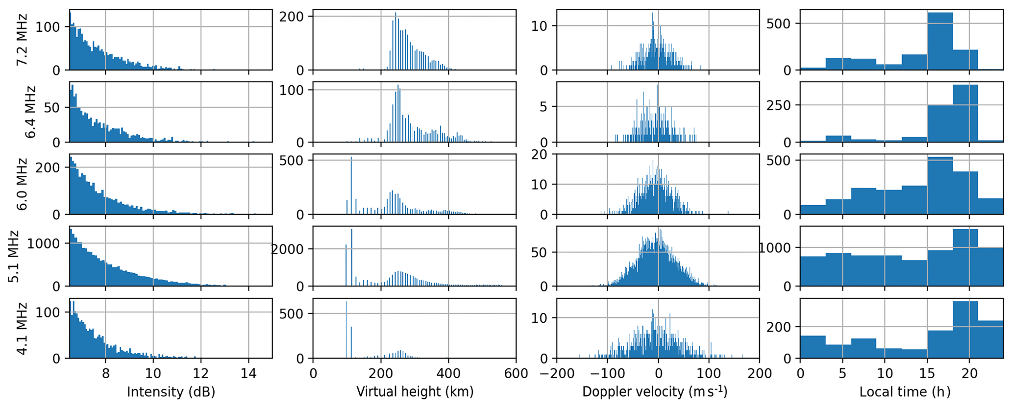
Figure 2 This figure shows histograms of received intensity, virtual height, Doppler velocity (positive for decreasing path lengths) and local time of received echoes.

3 Results

3.1 Results of the McMurdo–South Pole demonstration

The system was operated between 28 February and 13 March at 12 frequencies between 2.6 and 7.2 MHz. These are listed in Table 2. No signals were received below 4.1 MHz, due to absorption and reduced transmitter efficiency. No signal was received on 4.4 MHz for unknown reasons. Histograms of intensity, virtual height, and Doppler velocity of the working frequencies are shown in Fig. 2. The full range–Doppler–intensity time series are shown in the Supplement. The observed ranges and Doppler velocities are tightly clustered within physically realistic parts of the system's un-aliased observing scope, which covers more than 2500 km of virtual height and 3000 m s⁻¹ of Doppler velocity. The virtual heights show two distributions, with E- and F-layer echoes clearly separated on frequencies up to 6 MHz and only F-layer echoes (>200 km) at 7.2 MHz. The observed Doppler velocities are typically small with a small negative bias. The local time distribution of the echoes shows a clear peak between 15:00 and 21:00 LT on all frequencies, consistent with the expectation that sporadic-F should occur in the local afternoon or evening. The local time distribution may explain the negative Doppler bias, given that the F region tends to move upwards during this time interval.

Table 2 Number of ionospheric echoes received between 28 February and 15 March.

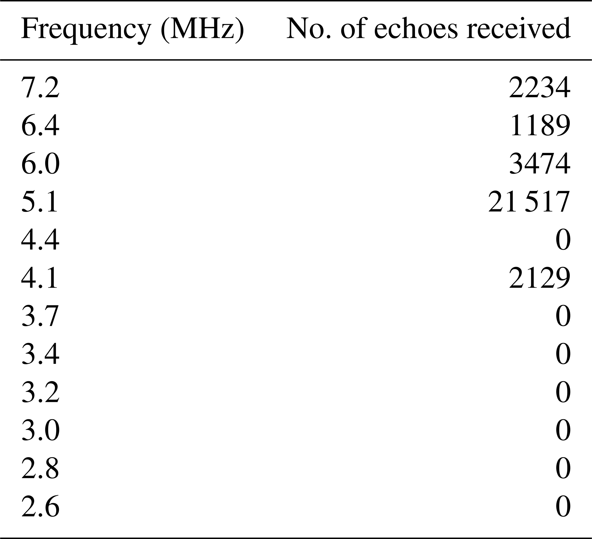
A total of 30 543 ionospheric echoes were received. Of the working channels, the largest number of echoes was received on 5.1 MHz and the least on 6.4 MHz. The number of echoes received on 5.1 MHz (21 517) is actually 25 % higher than the number of minutes in the test period (17 280) because echoes are frequently received at multiple ranges, from both the E and F layers at the same time. This multi-mode propagation is possible because the signal's angle of incidence is different for the two layers (larger for the E layer) and because the signal scatters. Multi-mode propagation can be seen clearly in virtual height–time–intensity data shown in Fig. 3, especially on 5.1 MHz. The E layer is clearly visible on 4.1, 5.1 and 6.0 MHz, with stable virtual height of 100–120 km. The F-region echoes, by contrast, exhibit sporadic variability on the higher frequencies. Some of these sporadic-F enhancements are spread in virtual height by 500+ km, most notably on 5.1 MHz.

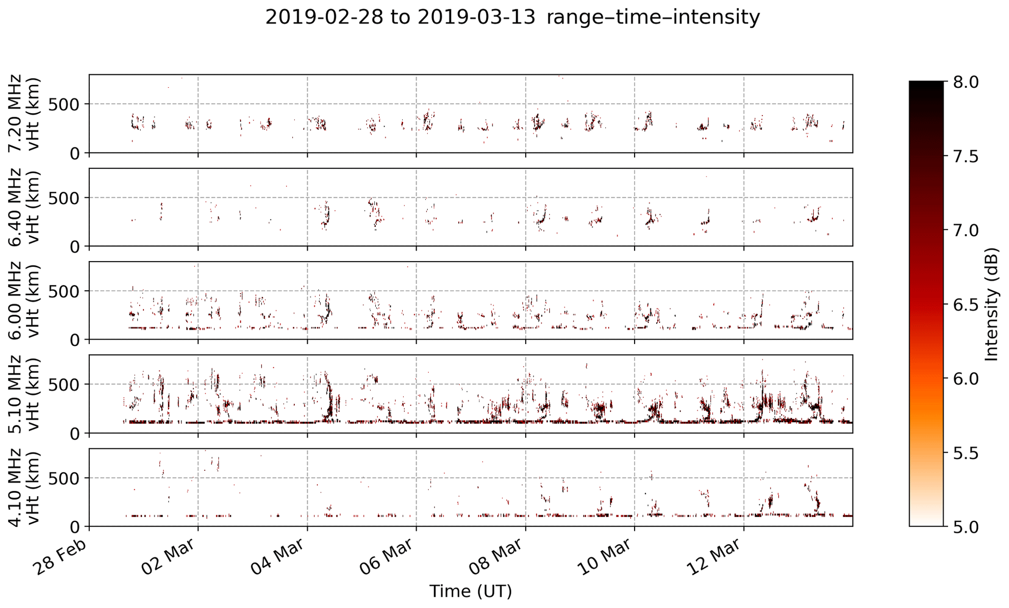
Figure 3 This figure shows virtual height–time–intensity data from the technology demonstration experiment (transmitter at McMurdo, receiver at South Pole). The E layer is consistently visible at 100–120 km on 4.1 and 5.1 MHz. Sporadic F-region enhancements are seen around local noon (UT+12) on the higher frequencies. These are accompanied by dramatic virtual height spreading of 500 km+.

3.2 Validation against Jang Bogo VIPIR

NmF2 from the McMurdo–South Pole experiment is compared against that observed by the Jang Bogo VIPIR in Fig. 4. The diurnal variability of NmF2 is consistent across both datasets, though the oblique experiment observes a smaller range of values due to its lower-frequency resolution. The Jang Bogo VIPIR reports more NmF2 values due to its higher sensitivity and due to the fact that it covers more frequencies.

Figure 4 This figure shows NmF2 from the McMurdo–South Pole oblique experiment (red) and Jang Bogo VIPIR (blue). The two datasets are consistent, but the McMurdo–South Pole experiment shows a smaller range of values because it uses fewer frequencies.

3.3 Comparison with ground-based GPS TEC

MIDAS TEC data at the reflection point are compared against the maximum-frequency (7.2 MHz) HF returns in order to determine whether observed density enhancements are correlated across the two datasets. High TEC values at the midpoint between McMurdo and the South Pole could be a predictor of maximum-frequency (7.2 MHz) links between the two stations because of the association between NmF2 (and therefore critical frequency) and TEC. A 6 TECU threshold was found to provide a good association with the 7.2 MHz propagation data. Several free parameters escape this comparison, notably variations in signal absorption from the D and E layers, scattering by irregularities, variations in the peak height (hmF2) and sub-grid-scale variability missed by the TEC images, so an exact match is not expected. Results are shown in Fig. 5. TEC >6 TECU predicts propagation successfully 40 % of the time, and TEC <6 TECU predicts absence of propagation 73 % of the time.

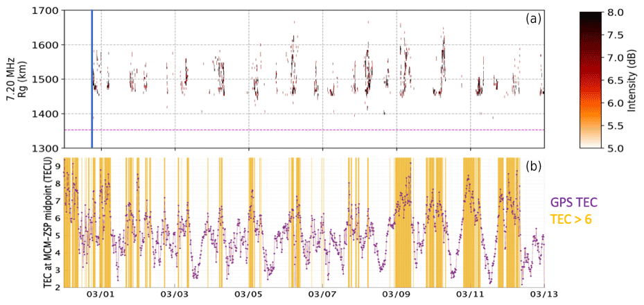
Figure 5 Panel (a) shows 7.2 MHz echoes from the McMurdo–South Pole demonstration and (b) MIDAS GPS TEC at the midpoint between McMurdo and the South Pole. TEC values >6 TECU are highlighted to illustrate the correspondence between TEC enhancements and sporadic F-region propagation. The time when the transmitter was switched on is shown in blue in (a).

4 Discussion

Data from the experiment indicate that the system performed successfully. Virtual height and Doppler distributions are physically realistic, indicating that the transmitter and receiver clocks and oscillators were synchronized correctly. The virtual height distributions show a clear separation between E- and F-layer echoes. The system's observing capability (>2500 km virtual height and 3000 m s⁻¹ total Doppler resolution) vastly exceeds the physically expected range of values, and the reported observations lie well inside the expected regions of the system. All these factors show that the reported echoes are real ionospheric reflections originating from McMurdo and received at South Pole. The NmF2 observations validate well against the Jang Bogo VIPIR data.

Propagation on 7.2 MHz was predicted moderately well by MIDAS GPS TEC (40 % true positive, 73 % true negative), given the inherent differences between the two datasets. This indicates that relatively high observed TEC can be considered a necessary but insufficient condition for predicting 7.2 MHz propagation between McMurdo and the South Pole. Variability beyond the spatiotemporal resolution of the available GPS TEC data may explain the disparity between the two datasets. Such mesoscale variability is known to be higher during times of enhanced F-region density, when steep ionospheric density gradients and high velocities are common. Other relevant factors include signal absorption by the D and E layers, peak height variations and scattering by irregularities.

Enormous spreading of virtual height is frequently observed. Echoes are received simultaneously across intervals of over 500 km virtual height. If the signal is instead being spread horizontally, these data could be interpreted as indicating azimuthal deviations of up to 35^∘ off of great-circle propagation (assuming a 200 km reflection height). This is on the order of the azimuthal spreads reported by Bust et al. (1994) and Flaherty et al. (1996) at middle and low latitudes.

5 Summary

A new oblique ionosonde has been developed and installed at McMurdo and South Pole stations. A 2-week system demonstration yielded over 30 000 ionospheric echoes indicating a stable E layer and a sporadic and variable F layer with dramatic range spreading. The experiment validates well against the Jang Bogo VIPIR vertical ionosonde and MIDAS GPS-derived TEC data. Given the success of this pilot experiment and the low cost of the equipment (∼ USD 15 000), this technology could be used to build a large network of ionospheric sounders operating multi-statically to provide new scientific insights into high-latitude ionospheric behavior. Such a network would dramatically expand the spatial coverage of ionospheric observations while requiring a relatively small number of new transmitters.