The use of the 1.27 µm O₂ absorption band for greenhouse gas monitoring from space and application to MicroCarb

Monitoring CO₂ from space is essential to characterize the spatiotemporal distribution of this major greenhouse gas and quantify its sources and sinks. The mixing ratio of CO₂ to dry air can be derived from the CO₂∕O₂ column ratio. The O₂ column is usually derived from its absorption signature on the solar reflected spectra over the O₂ A band (e.g. Orbiting Carbon Observatory-2 (OCO-2), Thermal And Near infrared Sensor for carbon Observation (TANSO)/Greenhouse Gases Observing Satellite (GOSAT), TanSat). As a result of atmospheric scattering, the atmospheric path length varies with the aerosols' load, their vertical distribution, and their optical properties. The spectral distance between the O₂ A band (0.76 µm) and the CO₂ absorption band (1.6 µm) results in significant uncertainties due to the varying spectral properties of the aerosols over the globe.

There is another O₂ absorption band at 1.27 µm with weaker lines than in the A band. As the wavelength is much closer to the CO₂ and CH₄ bands, there is less uncertainty when using it as a proxy of the atmospheric path length to the CO₂ and CH₄ bands. This O₂ band is used by the Total Carbon Column Observing Network (TCCON) implemented for the validation of space-based greenhouse gas (GHG) observations. However, this absorption band is contaminated by the spontaneous emission of the excited molecule O₂^*, which is produced by the photo-dissociation of O₃ molecules in the stratosphere and mesosphere. From a satellite looking nadir, this emission has a similar shape to the absorption signal that is used.

In the frame of the CNES (Centre National d'Études Spatiales – the French National Centre for Space Studies) MicroCarb project, scientific studies have been performed in 2016–2018 to explore the problems associated with this O₂^* airglow contamination and methods to correct it. A theoretical synthetic spectrum of the emission was derived from an approach based on A₂₁ Einstein coefficient information contained in the line-by-line high-resolution transmission molecular absorption (HITRAN) 2016 database. The shape of our synthetic spectrum is validated when compared to O₂^* airglow spectra observed by the Scanning Imaging Absorption Spectrometer for Atmospheric Chartography (SCIAMACHY)/Envisat in limb viewing.

We have designed an inversion scheme of SCIAMACHY limb-viewing spectra, allowing to determine the vertical distribution of the volume emission rate (VER) of the O₂^* airglow. The VER profiles and corresponding integrated nadir intensities were both compared to a model of the emission based on the Reactive Processes Ruling the Ozone Budget in the Stratosphere (REPROBUS) chemical transport model. The airglow intensities depend mostly on the solar zenith angle (both in model and data), and the model underestimates the observed emission by ∼15 %. This is confirmed with SCIAMACHY nadir-viewing measurements over the oceans: in such conditions, we have disentangled and retrieved the nadir O₂^* emission in spite of the moderate spectral resolving power (∼860) and found that the nadir SCIAMACHY intensities are mostly dictated by solar zenith angle (SZA) and are larger than the model intensities by a factor of ∼1.13. At a fixed SZA, the model airglow intensities show very little horizontal structure, in spite of ozone variations.

It is shown that with the MicroCarb spectral resolution power (25 000) and signal-to-noise ratio (SNR), the contribution of the O₂^* emission at 1.27 µm to the observed spectral radiance in nadir viewing may be disentangled from the lower atmosphere/ground absorption signature with a great accuracy. Indeed, simulations with 4ARCTIC radiative transfer inversion tool have shown that the CO₂ mixing ratio may be retrieved with the accuracy required for quantifying the CO₂ natural sources and sinks (pressure-level error ≤1 hPa; $X_{{\mathrm{CO}}_{\mathrm{2}}}$ accuracy better than 0.4 ppmv) with the O₂ 1.27 µm band only as the air proxy (without the A band). As a result of these studies (at an intermediate phase), it was decided to include this band (B4) in the MicroCarb design, while keeping the O₂ A band for reference (B1). Our approach is consistent with the approach of Sun et al. (2018), who also analysed the potential of the O₂ 1.27 µm band and concluded favourably for GHG monitoring from space. We advocate for the inclusion of this O₂ band on other GHG monitoring future space missions, such as GOSAT-3 and EU/European Space Agency (ESA) CO₂-M missions, for a better GHG retrieval.

1 Introduction

Carbon dioxide (CO₂) is recognized as the main driver of human-induced climate change. Its evolution in time is therefore scrutinized with attention. We know how much CO₂ is produced each year by human activity, but it does not correspond to the measured yearly increase of CO₂ in the atmosphere. The atmospheric fraction is the ratio of the atmospheric increase of CO₂ mass to the mass of CO₂ anthropogenic emission. On decadal timescales, this ratio has been close to 0.5 since the beginning of continuous measurements of atmospheric concentration in the late 1950s, despite an increase of the anthropogenic emissions by a factor of 5 (Le Quéré et al., 2018). An atmospheric fraction lower than 1 is explained by the existence of natural sinks that are fuelled by the increasing amount of CO₂ in the atmosphere. The current global carbon budget indicates that the ocean and land surface contribute roughly equally to the sink. There is little doubt that the oceanic sink will continue in the future despite a solubility decrease induced by raising temperature, while the fate of the land sink is more uncertain (Ciais et al., 2013). There is a lack of understanding of the vegetation dynamic, and its response to increasing CO₂ and changing climate. In fact, there is no consensus on whether the land sink is mostly in the tropics, midlatitudes, or boreal regions. This lack of understanding of the vegetation processes limits our ability to anticipate the carbon budget and thus the rate of climate change.

There is therefore a strong need for a better understanding of the carbon cycle and the processes that control the exchanges of carbon between the atmosphere, the vegetation, and the soil. This understanding can be obtained through a continuous monitoring of the CO₂ fluxes at the land–atmosphere interface and the analysis of its response to interannual climate anomalies. This objective suggests the development of a satellite monitoring system as recognized by the scientific community and several space agencies (CEOS, 2018).

The first satellites to be launched with the aim of monitoring the CO₂ cycle were Envisat (European Space Agency; ESA) with the Scanning Imaging Absorption Spectrometer for Atmospheric Chartography (SCIAMACHY) instrument, Greenhouse Gases Observing Satellite (GOSAT) (Japan Aerospace Exploration Agency; JAXA) and Orbiting Carbon Observatory (OCO) (NASA). The latter was unfortunately lost at launch, and a very similar satellite, OCO-2, was built and launched. These have been followed by TanSat (Chinese Academy of Sciences), GOSAT-2, and OCO-3 on the International Space Station. All instruments rely on a similar method to estimate the CO₂ concentration from space: high-resolution spectra of the reflected sunlight are acquired over several bands centred on clusters of CO₂ and O₂ absorption lines. The depths of the lines are sensitive to the number of molecules along the sunlight atmospheric path. The so-called differential absorption method makes it possible to infer the amount of absorbing gas along the line of sight, using some ancillary information on the atmospheric profile. CO₂ is the target component of the atmosphere and O₂ is used as a normalization component to link the CO₂ estimated number of molecules to a mixing ratio. Note that the sunlight atmospheric path length is linked to the surface pressure but also to the presence of light-scattering particles (aerosols and clouds) in the atmosphere. Because oxygen is well mixed in the atmosphere, it is adequate for the normalization of the measurement to estimate a mixing ratio.

The instruments currently in orbit focus on the CO₂ absorption bands at 1.6 and 2.0 µm, and the O₂ absorption band at 0.76 µm. The use of the oxygen band poses several challenges: (i) there is still significant uncertainty on the radiative transfer modelling within this band; and (ii) its central wavelength is notably different from that of the CO₂ bands so that the spectral variations of the atmospheric scatterer optical properties may lead to different optical paths for photons at different wavelengths.

An alternative could be the use of the O₂ absorption band around 1.27 µm. It is much closer in wavelength to the CO₂ absorption bands, which reduces the uncertainties linked to the spectral variations of the atmospheric path. In addition, the absorption lines are weaker than those in the 0.76 µm band, so the radiative transfer modelling is more accurate. In fact, the 1.27 µm band is the one used for the processing of TCCON (Total Carbon Column Observing Network, a ground-based network of high-resolution spectrometers observing the Sun to determine column densities) spectra for the estimation of the column mixing ratio. This band was not selected for current flying CO₂ monitoring missions because it is affected by airglow, a light emitted by oxygen molecules in the high atmosphere. Oxygen airglow at 1.27 µm has a spectrum that is very similar to the oxygen absorption spectrum used to estimate the sunlight atmospheric path.

Figure 1 Sketch of a space instrument and platform to monitor greenhouse gases (GHGs), including CO₂. The O₂ concentration (black curve) and the O₂^* volume emission rate of the 1.27 µm airglow (blue curve) are plotted as a function of altitude. The optical path of nadir-viewing observations is inevitably crossing the airglow layer, whose emission is superimposed on the spectrum of solar radiation scattered by the surface–aerosols–atmosphere system. The O₂ absorption at 1.27 µm is mainly produced in the lower atmosphere, while the airglow is in the range of ∼30–70 km altitude. Ozone photolysis indicated in the figure is the main source of O₂ airglow at 1.27 µm but not the only one.

Previous studies (Kuang et al., 2002) conducted during the preparation phase of the OCO mission (Crisp et al., 2004) indicated that the contribution of airglow could not be corrected with the desired accuracy. Conversely, similar studies performed during the design phase of the CNES (Centre National d'Études Spatiales – the French National Centre for Space Studies) MicroCarb mission indicated that the airglow could be distinguished from the oxygen absorption spectrum, provided that the instrument achieve a high spectral resolution. These unpublished studies led to the addition of a fourth band, centred at 1.27 µm, in the MicroCarb optical concept. The MicroCarb mission shall then be the first CO₂ monitoring mission to test the potential of the 1.27 µm band, rather than the 0.76 µm band, for the estimate of CO₂ column concentrations from space. Note that the instrument does record the classical O₂ band at 0.76 µm for reference and comparison with previous space missions. Recently, an independent study (Sun et al., 2018) confirmed the MicroCarb analysis. The authors show that, indeed, airglow has a spectral signature that is different from that of the oxygen absorption and can therefore be distinguished from the signature of oxygen absorption. It argues for the inclusion of the 1.27 µm band in the design of future CO₂ monitoring missions. In the present paper, we describe the analysis of the airglow signature that has been conducted in the context of the MicroCarb preparation.

When describing the choices made to define the OCO investigation to determine CO₂ vertical columns and mixing ratios from nadir-viewing observations (which needs associated O₂ columns), Kuang et al. (2002) recognized the virtues of the O₂ band at 1.27 µm (closest to the CO₂ bands) but discarded its use because it is contaminated by the intense O₂ airglow dayside emission when looking nadir from an orbiter (Fig. 1). They quoted Noxon (1982) as having shown that the emission is not only intense but variable. In fact, Noxon (1982) analysed spectra of this emission collected from 60 flights of a KC-135 aircraft over 10 years and a variety (latitude and seasons) of observing conditions, including two solar eclipses. He reported that there were no secular variations (within 30 %), and also that the variations with latitude (obtained along a single flight) were very smooth. This smoothness is confirmed by the present study of both the SCIAMACHY dataset and the airglow model that we made, combined with a chemistry transport model (CTM) model of ozone (not a climatology).

We have mentioned before that the TCCON ground-based spectrometer array, observing the Sun, uses this 1.27 µm band to derive the CO₂ ∕ dry air mixing ratio (because the O₂ ∕ dry air mixing ratio is fixed equal to 0.2095) rather than the A band, which can also be measured by some TCCON spectrometers. Why? The argument is that the depth of the O₂ lines at 1.27 µm has the same order of magnitude as those of CO₂, while the A-band (760 nm) absorption lines are much stronger. The use of spectral bands with similar absorption depth may reduce small systematic errors (e.g. detector linearity failure) for atmospheric quantities that are based on measurement ratios. We argue that the same argument can be used for observations from space, although other problems are added (Ring effect of filling the line bottoms, polarization, etc.).

Given the level of accuracy which is needed for a useful retrieval of CO₂, it may not be possible to rely only on an a priori model of the O₂ airglow to subtract it from a nadir-viewing spectrum which contains both the absorption spectrum of O₂ and the emission spectrum at 1.27 µm, closely blended. An exception may be for high-surface-reflectance scenes, such as glint viewing, when the transmitted reflected signal gets much larger than the airglow emission. Indeed, for typical scenes, the amplitude of the reflected and airglow spectra are similar, with nearly identical spectral variations. There are nonetheless some differences that make it possible to disentangle one from the other. First, there is the collision-induced absorption (CIA) which is present in absorption but not in emission, since it is proportional to the square of the O₂ density and therefore confined to lowest altitudes. Second, the emission at 1.27 µm increases linearly with the column of O₂^* at all wavelengths (re-absorption by O₂ is negligible at emission altitude), resulting in a constant relative shape of the emission spectrum, while the absorption spectrum is not linear: the transmittance $\text{Tr}=\text{exp}(-\mathit{\tau })$ saturates at high optical thicknesses of O₂ τ>1, and the absorption spectral shape is not constant but depends on the air-mass factor. Third, individual rotational lines are subjected to pressure broadening, also proportional to the air density. Therefore, the emission lines occurring at high altitudes are much thinner than the same absorption lines built in the lower atmosphere. These effects are illustrated in Fig. 2. O'Brien and Rayner (2002) have proposed to discriminate the emission from the absorption by recording a single line at very high spectral resolution (resolving power of 400 000), with an imager and three very narrow filters, whose positions are indicated in Fig. 2. One difficulty with this scheme is that the photon flux collected in those three narrow bands is very small and the corresponding signal-to-noise ratio (SNR) strongly reduced, rendering this proposal unpractical. By contrast, the size of a pixel element of MicroCarb (corresponding to a resolving power of 25 000) is also indicated for comparison. The whole spectrum is recorded, and the shoulders of the absorption line contribute to the disentangling of emission and absorption in a retrieval exercise, with 1024 pixels distributed along the O₂ band.

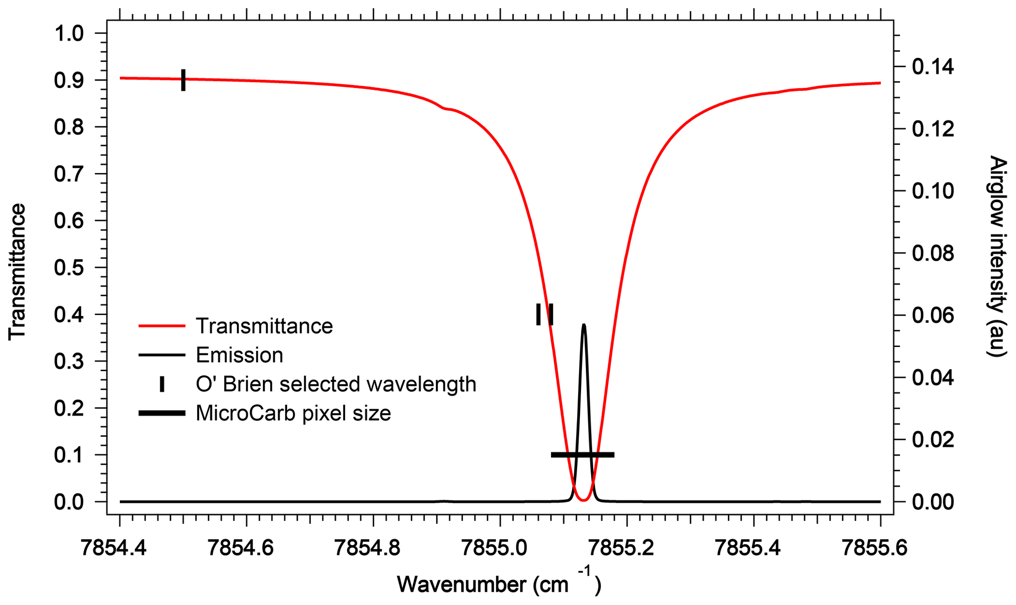
Figure 2 Comparison at high spectral resolution of spectral shape of atmospheric O₂ transmission (transmittance) and spectral shape of O₂^* emission. The full width at half maximum (FWHM) of an individual O₂ line (red) is much wider than the FWHM of its counterpart in emission (black line), allowing in principle to disentangle absorption from emission at selected wavelengths. The channels recommended by O'Brien and Rayner (2002), of width 0.02 cm⁻¹, are represented: one outside an O₂ line for the continuum; the other two on the side of an absorption line but still outside the airglow emission line. The transmittance was calculated with HITRAN at nadir at highest spectral resolution. The black line represents the MicroCarb pixel size, giving a resolving power of 25 000.

This paper is organized as follows. In Sect. 2, a brief review of previous observations of the O₂ (0, 0) airglow emission at 1.27 µm is presented first and a formula for computing a theoretical airglow spectrum is given. In Sect. 3, we describe how the SCIAMACHY observations of this airglow at the limb have been processed in order to derive volume emission rate (VER) vertical profiles (vertical inversion), and how a synthetic airglow spectrum may be derived from combining the VER profile and our spectroscopic studies. Our model spectral shapes are validated by a comparison with SCIAMACHY observed shapes. In Sect. 4, we compare the airglow total nadir intensities and VER profiles derived from SCIAMACHY limb observations with our Reactive Processes Ruling the Ozone Budget in the Stratosphere (REPROBUS) airglow model. A deficit of airglow from the model is found. The MicroCarb space mission with its instrument is briefly described in Sect. 5. It is shown in Sect. 6 that the O₂ airglow emission may be extracted from nadir-viewing SCIAMACHY observations over the oceans, where the reflectance is minimal, in spite of its moderate spectral resolution. Section 7 covers the overall conclusions with a prospective on future greenhouse gas (GHG) monitoring space missions.

We put some additional details in several appendices, in order to ease the reading of the most important results in the main text. Appendix A contains details of the theoretical derivation of the synthetic spectrum of the O₂^* airglow, together with a method to accurately compute the shape of the airglow spectrum. The method of vertical inversion of the limb observations to retrieve a vertical profile of the airglow emissivity is described in Appendix B (onion peeling accounting for O₂ absorption). A comparison (Appendix C) of the ozone predicted by REPROBUS with Global Ozone Monitoring by Occultation of Stars (GOMOS)/Envisat observations indicates a model deficit in ozone which, when accounted for, would narrow the discrepancy between SCIAMACHY and the airglow model. In Appendix D, the accuracy and bias results of the O₂ column retrievals (or surface pressure) and O₂ airglow intensity disentangling from nadir MicroCarb simulated spectra are detailed in some typical situations. In Appendix E, some other cases where absorption measurements could be contaminated by airglow emission are examined in nadir viewing. In Appendix F, some corrections made to SCIAMACHY level-1c spectra to extract the absolute spectral radiance are illustrated.

2 Observations and spectroscopy of the O₂ airglow band at 1.27 µm

2.1 Observations of the airglow of O₂^* emission at 1.27 µm

The aeronomical emission at 1.27 µm was first observed in 1956, in the “dayglow” (daytime aeronomical emissions) from instruments aboard Soviet stratospheric balloons (up to 30 km altitude) (Gopshtein and Kushpil, 1964), but its origin was not understood at that time. Noxon and Vallance Jones (1962) recorded spectra from a KC-135 plane flying at 13 km altitude and described the origin of the emission in the form of the electronic transition of the oxygen molecule from an excited state to the fundamental, with the emission of a photon in one of the rotating branches of the (0, 0) transition that form the entire “1.27 µm atmospheric IR band”:

$$\begin{array}{}\text{(1)}& {\mathrm{O}}_{\mathrm{2}}\left(a^{\mathrm{1}}{\mathrm{\Delta }}_g\right)⟶{\mathrm{O}}_{\mathrm{2}}\left(X^{\mathrm{3}}{\sum }_g^{-}\right)+h\mathit{\nu }\left(\mathrm{1.27}\mathrm{\mu }\mathrm{m}\right).\end{array}$$

The recorded intensity was very large (more than 10 megarayleigh; 1 rayleigh is 10⁶∕4π photons cm⁻² s⁻¹ sr⁻¹), but atmospheric absorption in the very same band absorbs most of it before reaching the ground. The much fainter emission from the (0, 1) transition of the same electronic state at 1.58 µm had been observed earlier from the ground, because it is not attenuated by O₂ absorption (most O₂ molecules are in the $V^{\prime \prime }=\mathrm{0}$ vibration level at atmospheric temperatures). Throughout this paper, we use for convenience indifferently O₂^* or O₂(¹Δ) or O₂ (a¹Δ_g) to designate the molecule in its excited electronic state (a¹Δ_g). There are various ways to produce an O₂ molecule in its excited state (a¹Δ_g), which are schematized in Fig. 9. The most important mechanism of production of these excited molecules is the photolysis of ozone by solar UV:

$$\begin{array}{}\text{(2)}& {\mathrm{O}}_{\mathrm{3}}+h\mathit{\nu }\left(\mathit{\lambda }\le \mathrm{310}\text{nm}\right)⟶\mathrm{O}\left({}^{\mathrm{1}}D\right)+{\mathrm{O}}_{\mathrm{2}}\left(a^{\mathrm{1}}{\mathrm{\Delta }}_g\right),\end{array}$$

which therefore occurs during the day but can be observed more easily from the ground at dusk with a high intensity of 30 megarayleigh. Once it is produced, it remains there with a long lifetime, about 75 min, and is spontaneously de-excited by emitting a photon or by a collision without a photon (“quenching”).

At night, the emission falls to 100 kilorayleigh, but this time the origin of the molecules a¹Δ_g is mainly due to the recombination of oxygen atoms O in their electronic ground state O(³P):

$$\begin{array}{}\text{(3)}& \mathrm{O}+\mathrm{O}+M⟶{\mathrm{O}}_{\mathrm{2}}\left(a^{\mathrm{1}}{\mathrm{\Delta }}_g\right)+M.\end{array}$$

2.2 Space observations of 1.27 µm

With a sounding rocket, Evans et al. (1968) were able to reconstruct for the first time the vertical distribution of the emission at 1.27 µm, by inverting the brightness integral. Their VER profile showed that emissivity is highest at about 50 km (∼10⁷ photons cm⁻³ s⁻¹) and zero or low below 30 km (due to quenching and screening of solar UV by ozone). A secondary maximum at about 85 km is due to the presence of a layer of mesospheric ozone well documented by GOMOS/Envisat in star occultation mode of observation (Kyrölä et al., 2018).

Several satellite instruments have been used in the past for the study of the O₂(¹Δ) emission, mainly to retrieve the O₃ or the O concentration in the upper atmosphere:

• the Solar Mesosphere Explorer (SME) satellite (Thomas et al. 1984);

• the Optical Spectrograph and InfraRed Imager System (OSIRIS) spectrometer on the Odin satellite (Llewellyn et al., 2004);

• one infrared radiometer aboard the OHZORA satellite (Yamamoto et al., 1988);

• the SABER broadband IR photometer aboard the NASA Thermosphere, Ionosphere, Mesosphere Energetics and Dynamics (TIMED) aeronomy mission (Russell et al., 1999; Mlynczak et al., 2007; Gao et al., 2011); and

• the SCIAMACHY spectrometer experiment aboard the Envisat ESA mission (2002–2012) (Burrows et al., 1995; Bovensmann et al., 1999), which we analyse in Sects. 3 and 4.

2.3 Spectroscopy and modelling of a synthetic spectrum of O₂^* airglow

The spectroscopy of the O₂ molecule and the modelling of a synthetic spectrum of the O₂^* airglow are described with some details in Appendix A. We relied on the high-resolution transmission molecular absorption (HITRAN) spectroscopic database, both to illustrate the structure of P, Q, and R branches of the 1.27 µm electronic transition and to verify a theoretical relationship between the absorption and the emission in this band. By using some equations from the paper of Simeckova et al. (2006), which describes how were obtained the parameters contained in HITRAN database, we obtained a very simple result on the ratio of emission ε(k) to absorption line strength S_ν(k, T) for each spectral line (transition) k:

$$\begin{array}{}\text{(4)}& {\displaystyle \frac{\mathit{\epsilon }\left(k\right)}{S_{\mathit{\nu }}(k,T)}}=\mathrm{8}\mathit{\pi }c{\mathit{\nu }}_{\mathrm{0}}^{\mathrm{2}}{\displaystyle \frac{Q_{\text{tot}}\left(T\right)}{Q_{\text{tot}}^{\text{up}}\left(T\right)}}{\displaystyle \frac{\mathrm{1}}{\exp \left(\frac{{\text{c}}_{\mathrm{2}}{\mathit{\nu }}_{\mathrm{0}}}{T}\right)-\mathrm{1}}}.\end{array}$$

This equation is the same as Eq. (A13) of Appendix A. T is the temperature of the atmosphere in which is produced the airglow, ν₀ is the wavenumber of the transition, and c₂ is the second radiation constant, ${\mathrm{c}}_{\mathrm{2}}=\mathrm{h}c/{\mathrm{k}}_{\mathrm{B}}$, where c is the speed of light, h is the Planck constant, and ${\mathrm{k}}_{\mathrm{B}}=\mathrm{1.38065}\times {\mathrm{10}}^{-\mathrm{23}}$ J K⁻¹ is the Boltzmann constant. Q_tot(T) is the total internal partition sum of the absorbing gas at the temperature T, and $Q_{\text{tot}}^{\text{up}}\left(T\right)$ is the internal partition sum of the upper level (here, a¹Δ_g).

We have used this formulation to transform an absorption spectrum by O₂ that can be easily computed with Line-By-Line Radiative Transfer Model (LBLRTM) software (see details in Appendix A) into a synthetic emission spectrum. This method of construction of a synthetic emission spectrum was the basis of our work on three topics: a satisfactory comparison with the observed spectra of SCIAMACHY (see below); retrieving the airglow intensity from SCIAMACHY nadir data over low-albedo regions; retrieving the surface pressure from simulations at high spectral resolution.

We should mention that one reviewer was able to show with some manipulations of equations that the same relationship (Eq. 4) could be obtained from the equations contained in Sun et al. (2018). It clearly stands as a validation of our present work and shows that the two approaches are consistent. We should also mention that, in an early phase of our studies, we used what we call later below (Sect. 3.3) our “crude model”, in which the airglow emission spectrum would have the same spectral shape as the local emission spectrum. In Sect. 3.3, we show that SCIAMACHY data are in agreement with our “new” model, based on Eq. (4), rather than with the crude model.

3 The use of SCIAMACHY data for the study of the O₂ (¹Δ) emission

We have used the SCIAMACHY data because of the spectral capability (with a resolving power $\mathit{\lambda }/\mathrm{d}\mathit{\lambda }\sim \mathrm{850}$) and extensive dataset produced during the ESA/Envisat mission.

3.1 Description of SCIAMACHY investigation of O₂ (¹Δ) emission

SCIAMACHY is a multi-channel spectrometer dedicated to the study of Earth's atmosphere aboard the ESA Envisat satellite (Burrows et al., 1995, Bovensmann et al., 1999). It is an eight-channel grating spectrometer that measures scattered sunlight in limb and nadir geometries from 240 to 2380 nm. In addition, it was operated also in solar and lunar occultation. In this study, we have used both limb and nadir measurements covering the O₂(¹Δ) band (1230–1320 nm) in spectral channel 6 (1050–1700 nm).

In a recent study to retrieve the volume emission rates of O₂(¹Δ) and O₂(¹Σ) in the mesosphere and lower thermosphere, Zarboo et al. (2018) have used a special mode of SCIAMACHY: the mesosphere and lower thermosphere (MLT) limb scan mode, dedicated to the study of the mesosphere and lower thermosphere in the region of 50–150 km. This mode was used only twice a month from July 2008 until April 2012. In contrast, we have used the normal limb-mode viewing geometry, where SCIAMACHY tangentially observes the atmosphere from the surface up to about 100 km with a vertical step of 3.3 km. At each tangent point, the full width at half maximum (FWHM) of the field of view (FOV) is 2.6 km (with a somewhat coarser vertical resolution), the horizontal along-track resolution is about 400 km, and the horizontal cross-track resolution is 240 km. To improve the SNR, the four cross-track spectra at the same elevation step are co-added, reducing the cross-track resolution to 960 km (the swath width).

To generate data for our study, we used the SCIAMACHY level-1b version 8.02 dataset that we converted into level-1c radiometrically calibrated radiances (in physical unit) by using the SCIAMACHY command line tool SciaL1c version 3.2. Before deriving the O₂(¹Δ) VER profiles, we had to perform a few corrections on the level-1c radiance spectra, as illustrated in Appendix F. First we subtracted the average of the 4 spectra measured above 105 km tangent height (generally around 150 or 250 km) as a dark spectrum from the measured spectra at all of the other tangent heights. This high-altitude spectrum contains some residual spectral (readout) patterns left from the calibration step. All spectra contain two bad pixels at wavelengths of 1262.267 and 1282.128 nm. In order to correct these two pixels, we replaced their value by the average of their two surrounding pixels. When the tangent altitude of the line of sight (LOS) decreases, there is an increasing background signal due to the Rayleigh and/or aerosol scattering outside the O₂ band. We corrected the spectra from this signal by removing a straight line computed as a linear interpolation between the two “surrounding” average backgrounds (estimated from the median value of all points to avoid outliers) in the 1235–1245 nm domain and in the 1295–1305 nm domain. The spectra after correction are ready to be used for the retrieval of the SCIAMACHY O₂(¹Δ) VER, as described in Appendix B. An onion-peeling method, modified to account for the re-absorption of O₂, allows to retrieve the VER vertical distribution from any limb scan. Then the VER is integrated vertically, yielding the O₂(¹Δ) intensity that would be observed at nadir for an observer located at the tangent point of the limb scan.

In Fig. 3, the nadir radiances (equivalent to intensities or brightness) derived from a series of SCIAMACHY limb scans along one particular orbit are plotted as a function of solar zenith angle (SZA), when different atmospheric models are used (the atmospheric density profile modifies the re-absorption by O₂). For each model, there are two branches, corresponding to north and south along the dayside polar orbit of Envisat (the north branch is in winter, while the south branch is in summer for this orbit). We see that the choice of the atmospheric model in the computation of the O₂ absorption has a small (∼3 %) but noticeable impact (on the brightness seen at nadir). We have also plotted the prediction of the REPROBUS model, as described in Sect. 4 and 4.2.1. It should be noted that the choice of the “adapted climatology” (for which we take for each measurement the most appropriate in latitude and season of the three considered atmospheric models), makes it possible to reduce the separation between the two branches and thus to be closer to the separation between the two branches obtained with the REPROBUS model.

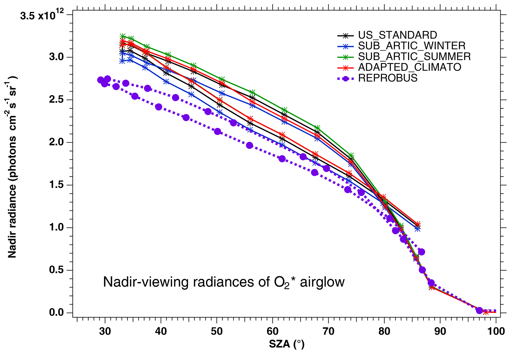
Figure 3 Computed O₂^* radiances in nadir-viewing geometry, derived from SCIAMACHY limb radiances, as a function of SZA for orbit 20070101_1256 when the O₂ absorption is computed with various choices of atmospheric models: climatology US_STANDARD (black), SUBARTIC_WINTER (blue), SUBARCTIC_SUMMER (green) and ADAPTED_CLIMATO (red) (see Appendix B for details). There is a slight dependence of the nadir intensity on the choice of atmospheric model. The dashed purple curve (with filled circles) corresponds to the REPROBUS v02 model.

3.2 Computation of synthetic spectra and comparison with SCIAMACHY observed spectra

Once we have the vertical profile of VER corresponding to a given SCIAMACHY limb scan, we can compute the spectrum of the local emissivity (in absolute units of photons cm⁻³ s⁻¹ sr⁻¹ nm⁻¹) with the theoretical approach developed in Appendix A. Then, we may integrate the spectra with Abel's integral along horizontal LOS tangent at the limb, for a direct comparison with the actually observed SCIAMACHY spectra. In this particular exercise, we did not account for the O₂ absorption for simplicity, and for this reason we restricted our comparison to altitudes >60 km. The spectral resolution of SCIAMACHY was used to smooth the high-resolution spectra (line by line) obtained from the approach described in Appendix A.

In Fig. 4a, the observed spectra, binned by altitudes (60–70, 70–80, and 80–90 km), are represented along with our model spectra computed for the same scans and binned in the same way, for a particular limb scan (points in green in Fig. F5 in Appendix F representing the locations of the tangent points of SCIAMACHY limb scans). The agreement is basically very good, both in shape and intensity. We note that the model is slightly brighter than the data, and the relative difference is larger for the bin 60–70 km than for the other bins. We tentatively assign this behaviour to the fact that we have not accounted for the O₂ absorption along the LOS in the model, more important at 60–70 km than higher.

Figure 4b is the same as Fig. 4a, with the crude model in which the spectral shape of the O₂^* emission is identical to the O₂ absorption. In this case, the R branch is systematically overestimated by this crude model.

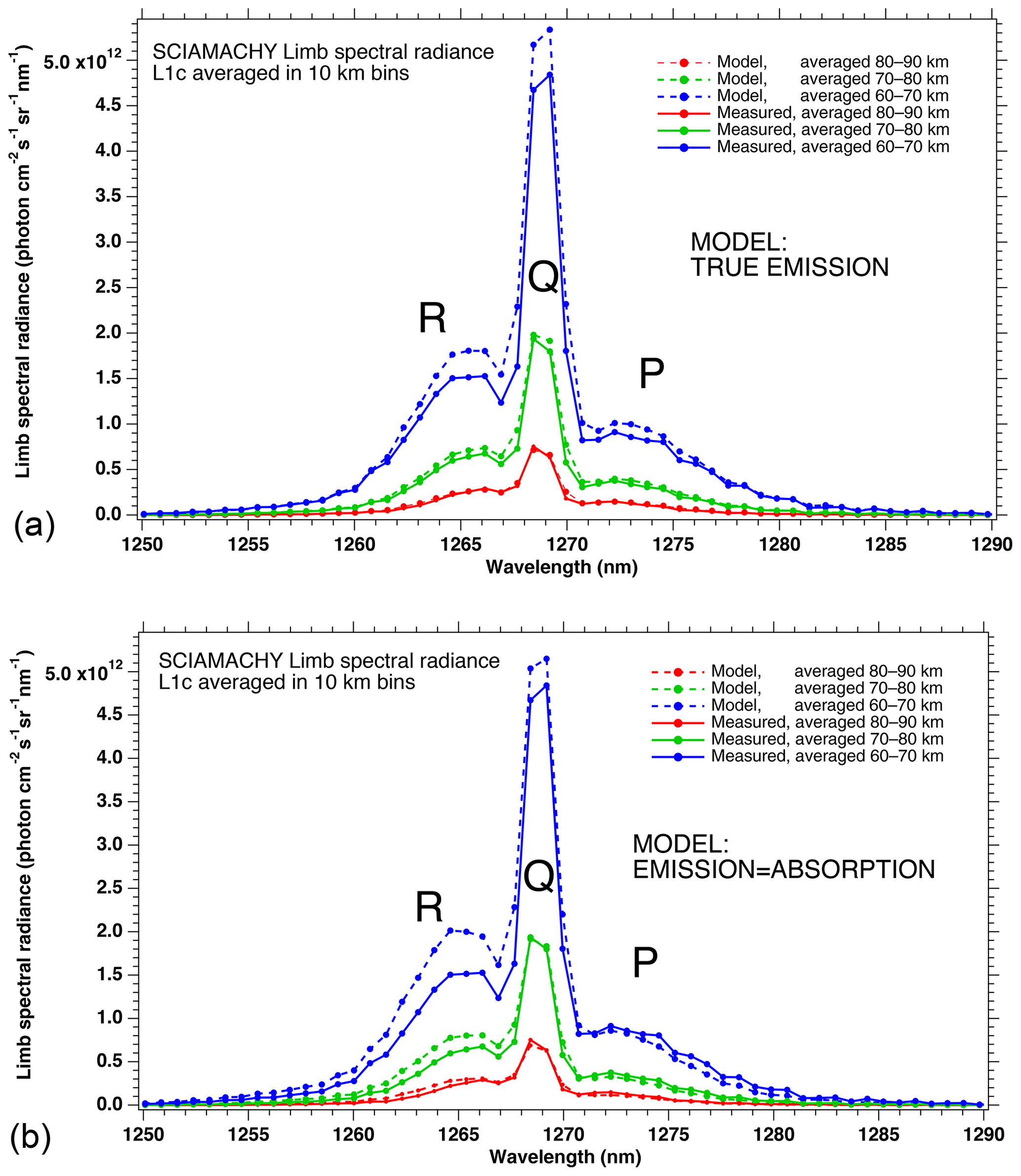
Figure 4 (a) SCIAMACHY limb spectra (solid lines; absolute units are photons cm⁻² s⁻¹ sr⁻¹ nm⁻¹), binned by altitudes (60–70, 70–80, and 80–90 km), along with our model spectra computed for the same scans and binned in the same way. Panel (b) is the same as (a) but with the crude model in which the shape of the emission of O₂^* is identical to the absorption by O₂. This crude model shows an excess of emission in the R branch (left) and a deficit in the P branch.

The ratio of measured spectra to model spectra (S_obs ∕ S_mod) were averaged together for all scans of that particular orbit within the same three altitude bins. They are represented in Fig. 5, both for the crude model (absorption equal to emission; Fig. 5a) and for our “true” model of emission based on Eq. (4) (Fig. 5b). It is clear that the crude model does not represent well the observed spectra, while the model with the true emission agrees quite well with the data. This comparison validates the approach that we developed in Sect. 2 and Appendix A, except that the overall level of the ratio is slightly below 1 (Fig. 5b). Again, we assign this behaviour to the fact that we have not accounted for the O₂ absorption along the LOS in the model, and indeed it can be seen that the ratios are closer to 1 for higher altitudes. Below 1255 nm and above 1285 nm, the intensity of the spectra is very small, and thus we attribute the noisy shape of the ratio spectra to low SNR.

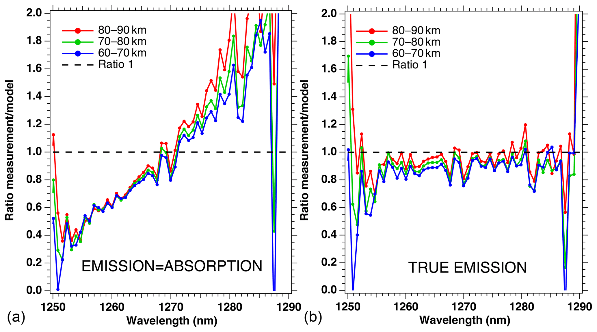
Figure 5 Ratios of measured spectra ∕ model spectra of limb spectra, averaged over a whole Envisat orbit, and binned by altitudes (60–70, 70–80, and 80–90 km). (a) Crude model in which the shape of the emission of O₂^* is identical to the absorption by O₂. (b) Same ratios with our new model described in Appendix A. The ratios are closer to 1 for larger altitudes because absorption by O₂ is neglected in this particular exercise.

3.3 Climatology of O₂^* VER derived from SCIAMACHY limb radiances

To build up a climatology of the O₂^* emission at 1.27 µm, we have applied our inversion scheme to get VER vertical distributions (Appendix B) to all SCIAMACHY limb data collected during the first 3 d of each month of 2007. Note that in the normal mode, the limb scans extend down to 0 km (our inversion is made >30 km), while in the special SCIAMACHY MLT mode, only altitudes >50 km are observed. Our database contains the analysis of 448 orbits, containing 12 400 limb scans in the normal mode which go down sufficiently for our purpose (some limb scans do not reach low enough altitudes to allow retrieval of the full VER profile above 30 km).

The vertical inversion of SCIAMACHY limb radiances to get a VER vertical profile is done below 90 km down to 0 km; but only results >30 km are significant, because at the limb and low altitudes, there is Rayleigh and aerosol solar radiation scattering (the useful signal for SCIAMACHY limb mode ozone retrieval) which dominates over the O₂^* radiance. Once a VER profile is obtained, it can be integrated vertically, taking into account the absorption by O₂. Therefore, a “SCIAMACHY” nadir radiance is obtained, which corresponds to the O₂^* radiance that would be observed by SCIAMACHY if it were observing nadir at the position of tangent points where the limb radiances were obtained. In fact, the nominal operation mode of SCIAMACHY does indeed alternate limb-viewing and nadir-viewing observations to discriminate tropospheric ozone from stratospheric ozone (Ebojie et al., 2014).

When this VER is integrated vertically to get a nadir radiance, the integration stops at the upper limit of 80 km in order to have a better comparison with the REPROBUS model which stops also at 80 km. The air atmospheric model selected to compute the re-absorption by O₂ is our so-called “adapted climatology” (see Appendix B). In Fig. 6, about one-third of all VER profiles collected for the first 3 d of January 2007 are displayed (other months are quite similar). The colour code corresponds to the SZA of the limb scan. We kept also scans near the terminator, where the VER is significant only above 80 km. Clearly, the SZA is the factor dominating the shape, the peak altitude and the intensity of the airglow VER profiles between 30 and 80 km. This is due to UV photo-dissociation of ozone (the main process of O₂^* production) penetrating more deeply when the SZA is small (because of ozone UV screening). The lower the SZA, the brighter the airglow emissivity. Above 80 km, other processes come into play and a second airglow peak is observed which seems less correlated with the SZA than is the main peak at 45–50 km. The altitude of the main airglow emissivity peak varies between 43 and 45 km for values of SZA below 50^∘ and increases for higher values of SZA up to about 60 km.

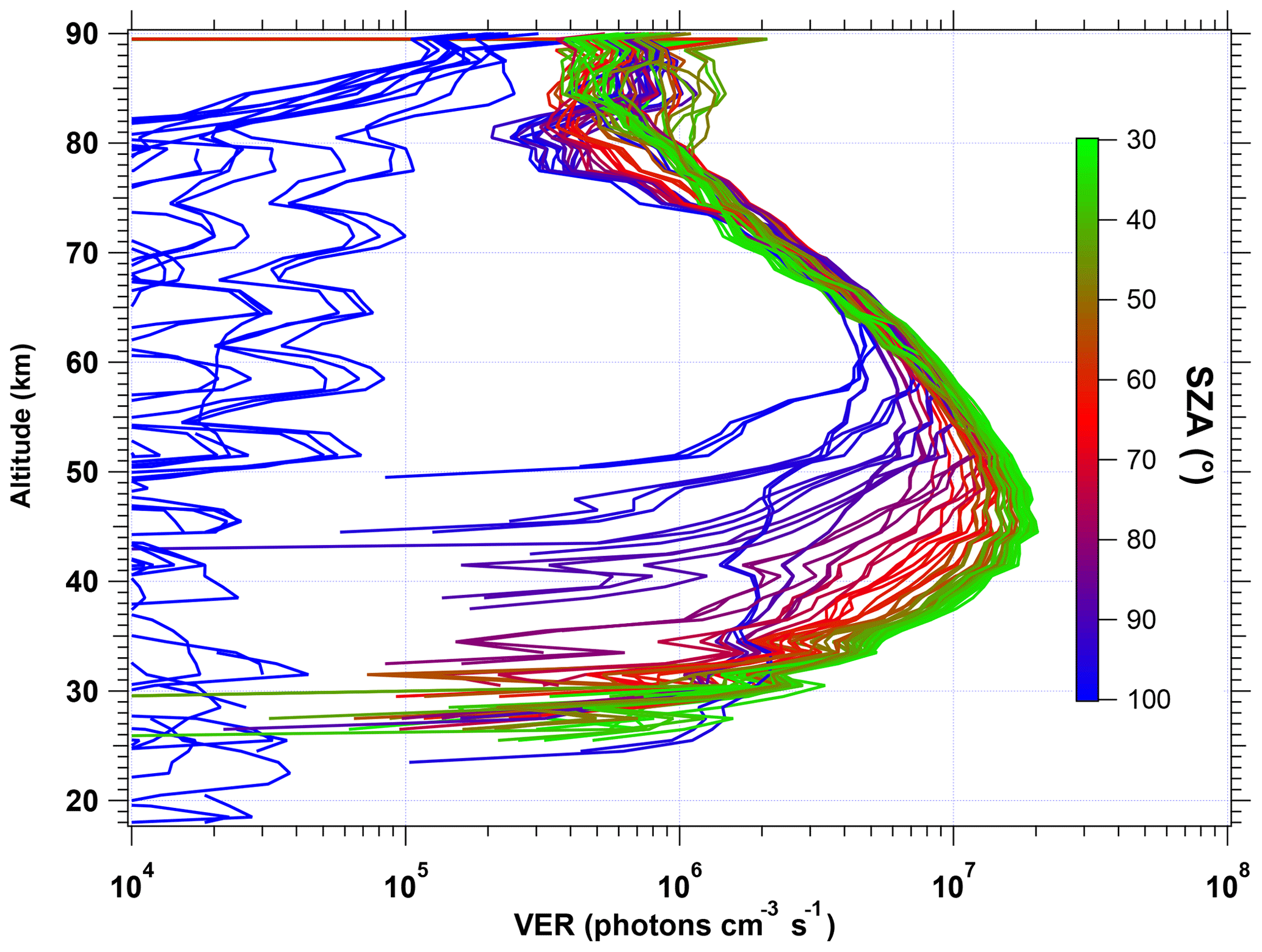
Figure 6 VER profiles of airglow at 1.27 µm retrieved from SCIAMACHY limb data for 1 January 2007 (80 profiles). The colour scale represents the SZA. For the lowest SZA values probed by SCIAMACHY (33^∘), the peak VER is 2×10⁷ photons cm⁻³ s⁻¹ around 45 km. At large SZA values, the emission is present only at high altitudes (>80 km). Above 90^∘, there is almost no signal for inversion.

In Fig. 7, all the “SCIAMACHY” nadir radiances (longitude–latitude) obtained by inversion of limb radiances and vertical integration of VER (first 3 d of each month of the year 2007) are mapped for 4 typical months, (January, April, July, and October). The airglow brightness is almost independent of longitude. At high latitudes (north and south), the brightness is lower: this is the effect of larger SZA. The region of maximum brightness is displaced with season, following the latitude of the sub-solar point, again an effect of the SZA dependence of the O₂^* radiance. This is illustrated in Fig. 8, where all the nadir radiances are plotted as a function of SZA, with a colour code on latitude. The lower SZA, the brighter is the nadir emission. This SZA dependence is well reproduced by the model (penetration of solar UV deeper in the ozone layer for small SZA; see Sect. 4). Still, there is a separation of the curves in two branches that are relevant to the Northern Hemisphere and Southern Hemisphere. The separation between the two branches depends on the season. This observed overall pattern of the O₂^* radiance is directly linked to the climatology of upper stratosphere/lower mesosphere ozone and also reproduced by the model (Sect. 4).

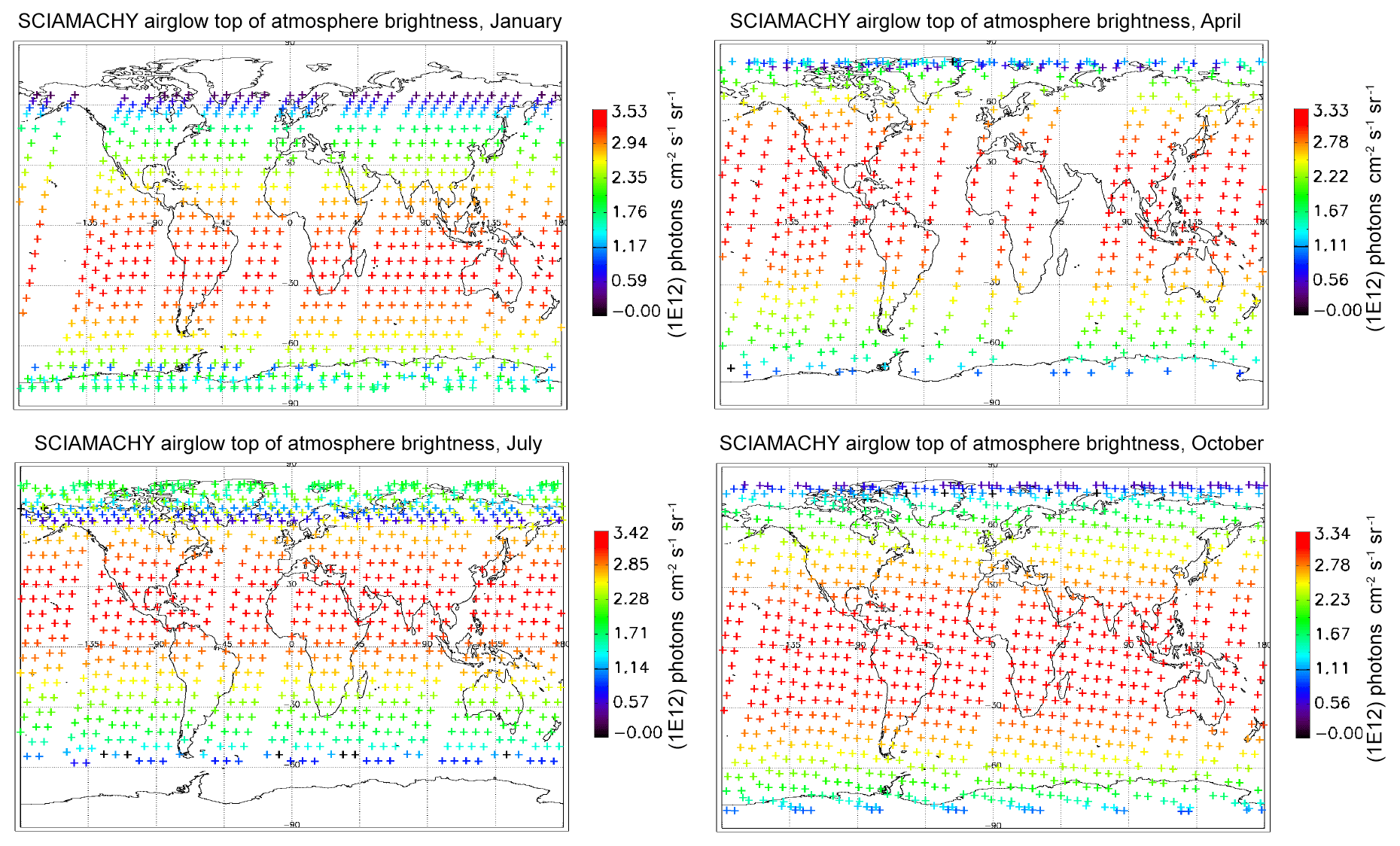
Figure 7 Airglow brightness maps as seen from space in nadir view, retrieved from SCIAMACHY limb-viewing data for the months of January, April, July, and October 2007 (first 3 d of each month only). The colour scale represents brightness. Zones without data (holes), particularly numerous in April, are corrupted products that have been eliminated. SZA points >90^∘ have been eliminated.

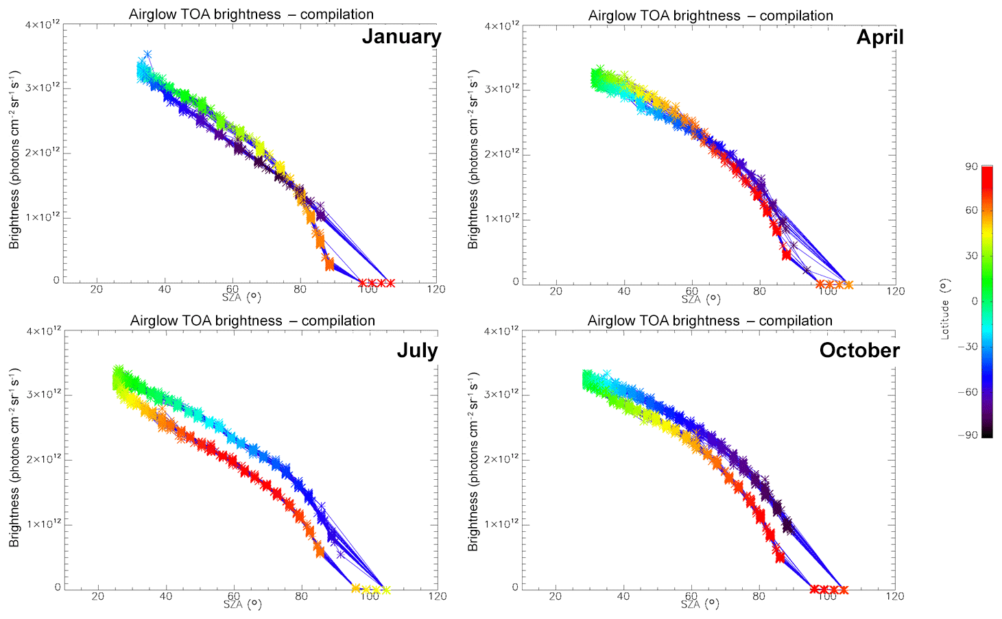
Figure 8 O₂^* airglow intensities that would be seen at nadir as a function of SZA for the months of January, April, July, and October 2007 (first 3 d of each month only), retrieved from the processing of SCIAMACHY limb data. The colour scale represents the latitude. There is a geometrical correlation between the latitude and SZA imposed by the polar orbit of Envisat. The airglow brightness is mostly correlated with SZA. The comparison of these intensities with those obtained by the REPROBUS airglow model is presented in Sect. 4.2.1.

4 Comparison between an airglow model based on REPROBUS and SCIAMACHY observations

In this section, we compare the predictions of a dedicated 3-D model of the airglow emission of O₂(a¹Δ_g) at 1.27 µm to the airglow observations of SCIAMACHY. The comparison makes use exclusively of the SCIAMACHY limb observations but is made in two different ways. One way is to compare the SCIAMACHY VER vertical profile retrieved from limb measurements through vertical inversion as described in Appendix B. The second way is to compare the nadir integrated emission I_ag (brightness) of the airglow. Both model and data nadir emissions are obtained by vertical integration of the VER, respectively, in the airglow model and in the SCIAMACHY-derived VER vertical profile. This nadir emission is directly relevant to the GHG observations since, from an orbiter and nadir viewing, this signal is superimposed on the solar back-scattered emission from which the columns of GHG gases and O₂ must be retrieved. This is why it is not practical to use the nadir observations of SCIAMACHY to study the O₂^* airglow, since the nadir signal is dominated by surface back-scattered solar radiation (except over the oceans, as we shall see in Sect. 6.2.2).

Since the photolysis of ozone is the major source of the O₂^* airglow, it was also felt necessary to compare the ozone density predicted by our airglow model and GOMOS ozone measurements also on Envisat, simultaneous with SCIAMACHY observations (but not with the same geometry), as described in Appendix C.

4.1 3-D simulation of the airglow emission of O₂(a¹Δ_g) at 1.27 µm

The airglow model is composed of two separated elements. The first element is the REPROBUS chemistry transport model (CTM) computing the 3-D distribution of ozone and other chemical species as a function of time, driven by analysed meteorological fields. The second element is an airglow model operated offline, which extracts from REPROBUS (for one location and one precise time and date) the information necessary for the computation of the relevant VER profile.

4.1.1 REPROBUS 3-D simulations

REPROBUS is a global CTM developed for the stratosphere (Lefèvre et al., 1994). It includes a complete description of stratospheric chemistry using 58 species and about 100 chemical reactions. The winds and temperatures used by REPROBUS are forced by the ECMWF operational analyses, over a domain that extends from the ground to 0.01 hPa (about 80 km) and a horizontal resolution of 2^∘ × 2^∘. For the present study, we carried out a REPROBUS simulation covering the whole year 2007 with the results saved every hour. The choice of 2007 was motivated by the fact that we had already extracted SCIAMACHY data for this year. From this new simulation, all the GOMOS or SCIAMACHY data obtained in 2007 can be compared to the CTM with a spatial difference less than or equal to 1^∘ and a time difference less than or equal to 30 min. It should be noted that for GOMOS the comparison with the model is limited to ozone profiles, since GOMOS does not have a channel at 1.27 µm and therefore does not observe airglow at this wavelength. SCIAMACHY observations of the 1.27 µm airglow were compared to the combination of REPROBUS and the offline airglow model.

Based on the results of REPROBUS available every hour of 2007 and the offline airglow model, we have developed a procedure for the automatic extraction of vertical ozone profiles and O₂(¹Δ) emission profiles as well as the integrated O₂(¹Δ) emission in coincidence with the GOMOS and SCIAMACHY measurements performed the same year. This dataset represents 4026 profiles modelled in coincidence with GOMOS and 12 800 in coincidence with SCIAMACHY. The statistical analysis of the comparison between the model and observations is presented in Sect. 4.2 for SCIAMACHY observations and in Appendix C for GOMOS observations. It should be noted that, as a result of some discrepancies revealed by this comparison, the REPROBUS model will be modified in the future for a better representation of mesospheric ozone. Although the retrieval of O₂ column does not need a model, it is likely that the output of the improved REPROBUS model (O₂^* intensity) will be used as a prior information in the retrieval process.

4.1.2 Simulation of airglow emission of O₂^* at 1.27 µm

Here, we do not care about the details of the spectral shape of the emission, but rather we compute the local emissivity (VER) and the vertically integrated emission, in order to compare with SCIAMACHY observations. The airglow at 1.27 µm is calculated offline from the 3-D outputs of the REPROBUS model. It takes into account all the mechanisms of production and loss of O₂(a¹Δ), as shown in Fig. 9. In practice, the O₂(¹Δ) emission model uses as input the ECMWF temperature and pressure profiles as well as the O₃ and O(³P) profiles calculated by REPROBUS for the selected date and location. From the pressure and temperature, the total density and density profiles of N₂, O₂, and CO₂ are also calculated. The airglow model then provides the vertical profiles of the mixing ratios of O(¹D), O₂(b¹Σ), O₂(¹Δ), the vertical profile of VER at 1.27 µm expressed in photons cm⁻³ s⁻¹, and the vertically integrated intensity expressed in photons cm⁻² s⁻¹ sr⁻¹ (brightness or intensity, directly comparable to the radiance signal of the solar radiation back-scattered by the gaseous atmosphere, aerosols and the surface).

Two versions of the airglow model were used. One early version of the model (v01) was later modified to a version v02 which yielded better agreement with SCIAMACHY observations. They differ only by the value of the quenching rate of the O₂(¹Δ). The early version v01 contained a quenching constant k:

$$\begin{array}{rl}& {\mathrm{k}}_{\mathrm{\Delta },{\mathrm{O}}_{\mathrm{2}}}=\mathrm{3.6}{e}^{-\mathrm{18}}\times \exp (-\mathrm{220}/T)\mathrm{in}{\mathrm{cm}}^{\mathrm{3}}{\mathrm{molecule}}^{-\mathrm{1}}{\mathrm{s}}^{-\mathrm{1}},\\ & T=\mathrm{temperature}\left(\mathrm{K}\right),\end{array}$$

recommended in the Jet Propulsion Laboratory (JPL) compilation (Burkholder et al., 2015). The version v02 has a slightly different value of k, recommended by the International Union of Pure and Applied Chemistry (IUPAC) (Atkinson et al., 2005):

$$\begin{array}{rl}& {\mathrm{k}}_{\mathrm{\Delta },{\mathrm{O}}_{\mathrm{2}}}=\mathrm{3.0}{e}^{-\mathrm{18}}\times \exp (-\mathrm{200}/T)\mathrm{in}{\mathrm{cm}}^{\mathrm{3}}{\mathrm{molecule}}^{-\mathrm{1}}{\mathrm{s}}^{-\mathrm{1}},\\ & T=\mathrm{temperature}\left(K\right).\end{array}$$

At stratospheric temperatures, the value of k${}_{\mathrm{\Delta },{\mathrm{O}}_{\mathrm{2}}}$ is decreased with v02 by about 10 %, enhancing the emission rate of O₂(¹Δ). This gives a better fit (but not perfect) between SCIAMACHY observations and the airglow model. According to Wiensz (2005), this IUPAC recommended value gives a better agreement between OSIRIS/Odin direct and indirect measurements of ozone. Unless otherwise specified, we are presenting in this paper the v02 results.

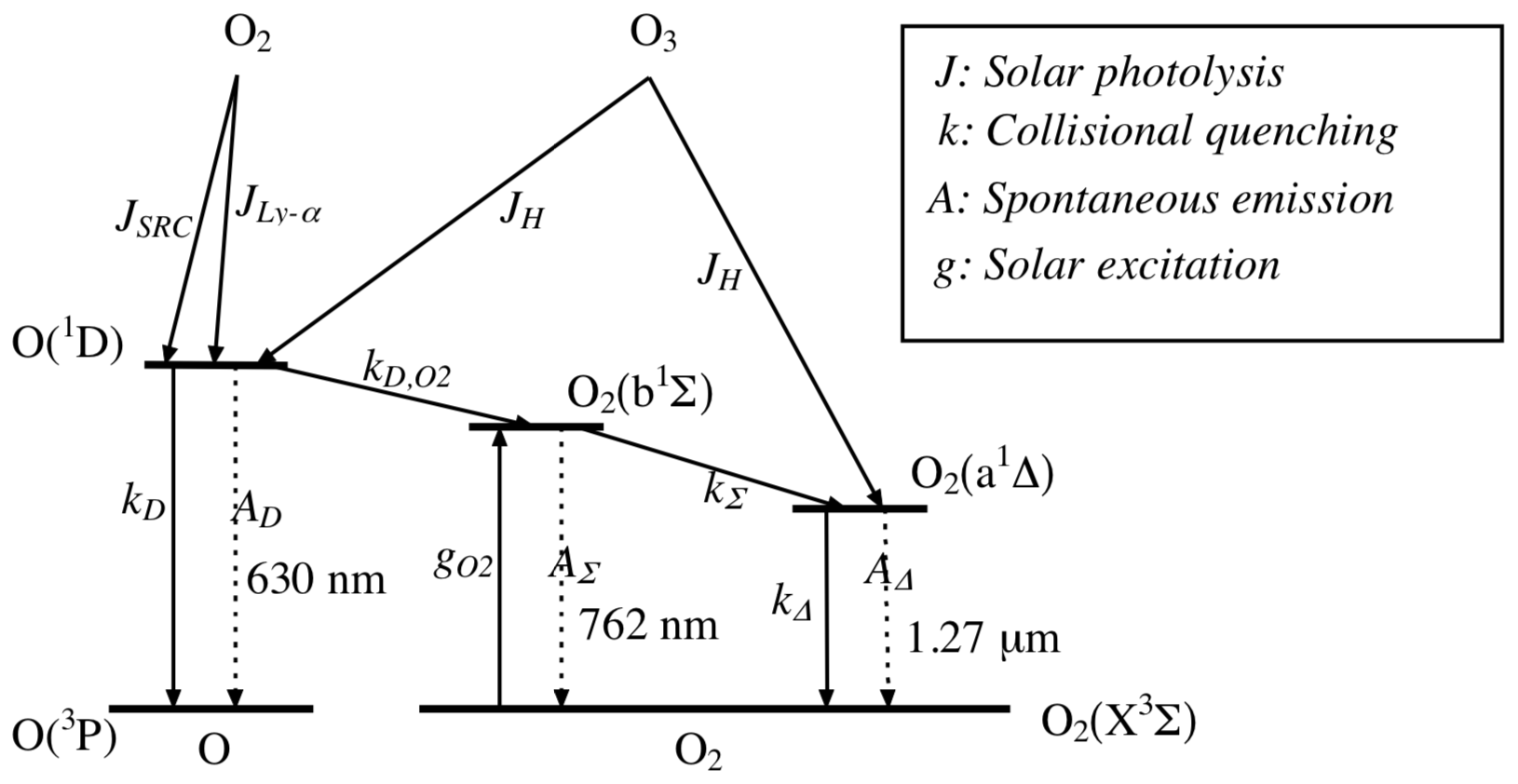
Figure 9 Energy diagram of the O and O₂ molecules showing both O₂ bands at 762 nm (A) and 1.27 µm. Only the O₂ photo-dissociation (J_SRC (Schumann–Runge continuum) and J_Ly−α) is not taken into account in our model, since this represents only about 1 % of the integrated emission (reproduced from Wiensz, 2005).

4.1.3 Some examples of model results

As an example, Fig. 10 shows the REPROBUS results for 21 June 2007 at the pressure level of 0.9 hPa (about 50 km), which corresponds to the altitude of maximum emissivity of O₂(¹Δ). The figure displays the O₃ volume mixing ratio (Fig. 10a), the corresponding volume emission rate of O₂(¹Δ) calculated by the airglow model (Fig. 10b), as well as the vertically integrated O₂(¹Δ) emission (Fig. 10c) (the possible reabsorption between the emission point and the top of the atmosphere by O₂ is here neglected).

On 21 June 2007, the volume emission rate of O₂(¹Δ) at 1.27 µm shows a maximum at high southern latitude that is obviously caused by a maximum of O₃ at the same location. However, the O₂(¹Δ) emission is very strongly modulated by the solar zenith angle. This effect is further exacerbated when the emission is vertically integrated: the intensity of the O₂(¹Δ) emission is then systematically maximum at local noon and its variations are entirely controlled by the solar zenith angle. At a given solar zenith angle, the intensity shows very little spatial variability and the effects of the heterogeneity of the ozone field are almost completely erased.

Figure 10 Simulations of the REPROBUS model for 21 June 2007 at 06:00 UT. This is the geographical distribution of three relevant quantities with their colour code. (a) Ozone mixing ratio (ppmv) at 0.9 hPa (about 50 km). (b) Volume emission rate of O₂(¹Δ) at 0.9 hPa in units of 10⁷ photons cm⁻³ s⁻¹. (c) Integrated vertical intensity of O₂(¹Δ) in units of 10¹² photons cm⁻² s⁻¹ sr⁻¹. Because of the particular time and date, the sub-solar point is at a latitude of 23.5^∘ N and on the meridian of 90^∘ E, which is the red spot plotted in the centre of panel (c).

4.2 Comparison of SCIAMACHY data with REPROBUS-derived airglow model

For each observation of our SCIAMACHY 2007 dataset in limb viewing, we have a co-located VER profile of O₂(¹Δ) calculated by the REPROBUS-based airglow model. We were therefore able to make comparisons between the airglow of SCIAMACHY and that of REPROBUS in two different ways: (i) the brightness of the airglow as it would be seen by a TOA (top-of-atmosphere) observer in nadir viewing; (ii) the VER airglow vertical profiles.

4.2.1 Comparison of O₂(¹Δ) airglow brightness as seen by a TOA observer in nadir view

The airglow model brightness is obtained by a vertical integration of the VER produced by the airglow model. Re-absorption by O₂ in nadir geometry is small and has been neglected. However, this nadir model intensity cannot be directly compared with a nadir observation of SCIAMACHY, as it is most of the time completely dominated by terrestrial albedo. Therefore, to evaluate the nadir intensity corresponding to the SCIAMACHY data in limb viewing, we proceeded as follows:

• For each vertical scan at the limb with SCIAMACHY, the total brightness of the airglow was first estimated by integrating spectrally the SCIAMACHY spectra at each altitude, and then the VER profile was determined with an onion-peeling method (taking into account horizontal re-absorption), as described in Appendix B.

• Then, the VER was vertically integrated to yield the intensity (or brightness) that an observer placed above the tangent points of the SCIAMACHY scan would see looking to nadir.

Figure 11 compares the nadir intensities as a function of SZA co-located for SCIAMACHY and REPROBUS for the first 3 d of January, April, July, and October 2007. This represents the data collected over ∼50 orbits of Envisat for each considered month. The Envisat orbit is almost polar and descending in latitude on the day side (Equator crossing around 10:30 LT, descending node). In both data and model, the SZA is the dominating factor for the intensity. The latitude (which is colour coded in the plot) plays also a small role (through the ozone field), more important in July. The repeatability of the SCIAMACHY-derived nadir intensities is obvious, with very little dispersion. The main difference between data and model is that at SZA ≲70^∘ the REPROBUS/airglow model systematically underestimates the airglow intensity by 10 %–20 % compared to that seen in the SCIAMACHY data.

Regarding the SZA of the SCIAMACHY data, we noted that the SZA value provided in the SCIAMACHY ESA products in limb viewing, as defined in the data product, is the SZA value of one of the two points (the nearest to Envisat) corresponding to the intersection between the LOS and TOA (defined at 100 km altitude). But what we need is the SZA of the tangent point of the LOS, which is different. Therefore, we systematically calculated the SZA at the tangent point of the SCIAMACHY LOS using an external tool (IDL routine). All results presented in this report are obtained using this recalculated SZA.

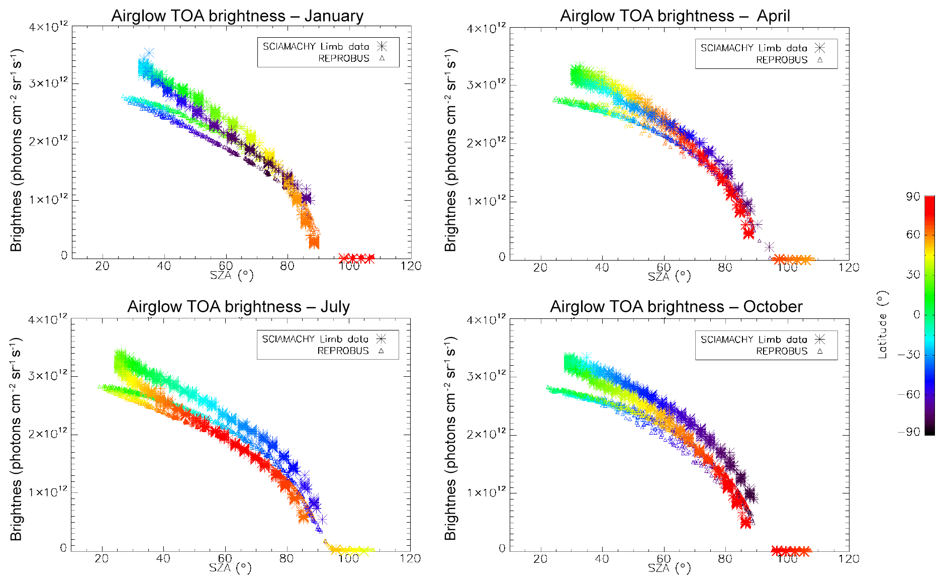
Figure 11 Airglow intensity seen at nadir as a function of SZA for the months of January, April, July, and October 2007 (first 3 d of each month only). Data (star symbol) come from the SCIAMACHY limb data (retrieval of VER with onion-peel inversion and subsequent vertical integration); other data (Δ symbol) are from the REPROBUS/airglow model. The colour scale for symbols represents latitude. The SZA for the SCIAMACHY curve was recalculated with an external tool. The data are systematically larger than the model but overall behaviour is similar.

Note that in Fig. 11 there is a remaining difference between the minimum SZA of the SCIAMACHY data and the minimum SZA of the model of up to about 8^∘. This difference may be explained due to the UT time difference between the model and the data since, unlike the data, the model was calculated on a fixed UT time grid with a round hour (10:00, 11:00 UT, etc.). There is therefore a time difference between model and data of up to 30 min, which can be both ways in difference of SZA: SZA(model) – SZA(data). The true SZA is the data one; and the model SZA may be the same as the data ± 8^∘, but only the negative differences of SZA(model) – SZA(data) are obviously visible on the plot, when SZA(data) is at its minimum value, and SZA(model) is below SZA(data). Points with positive differences are just mixed with all other points.

4.2.2 Comparison of VER vertical profiles

We have seen systematic differences between the nadir intensities (vertically integrated VER) of SCIAMACHY and REPROBUS. It is therefore interesting to pinpoint at which altitude the differences are essentially located, by directly comparing the vertical VER profiles produced by the REPROBUS model and those that could be derived from the SCIAMACHY limbs by onion-peel inversion. The comparison of some typical VER profiles of SCIAMACHY and REPROBUS is illustrated in Figs. 12 and 13. It shows that in the lower part of the profiles, say up to 40 km altitude, there is a good match of VER values between SCIAMACHY and REPROBUS. At higher altitudes >40 km, REPROBUS/airglow model predicts less O₂(¹Δ) airglow than observed by SCIAMACHY. One obvious possibility is that there would be actually more ozone in the upper stratosphere than predicted by the REPROBUS model, since the O₂^* emissivity is proportional to the ozone concentration at high altitudes (optically thin medium).

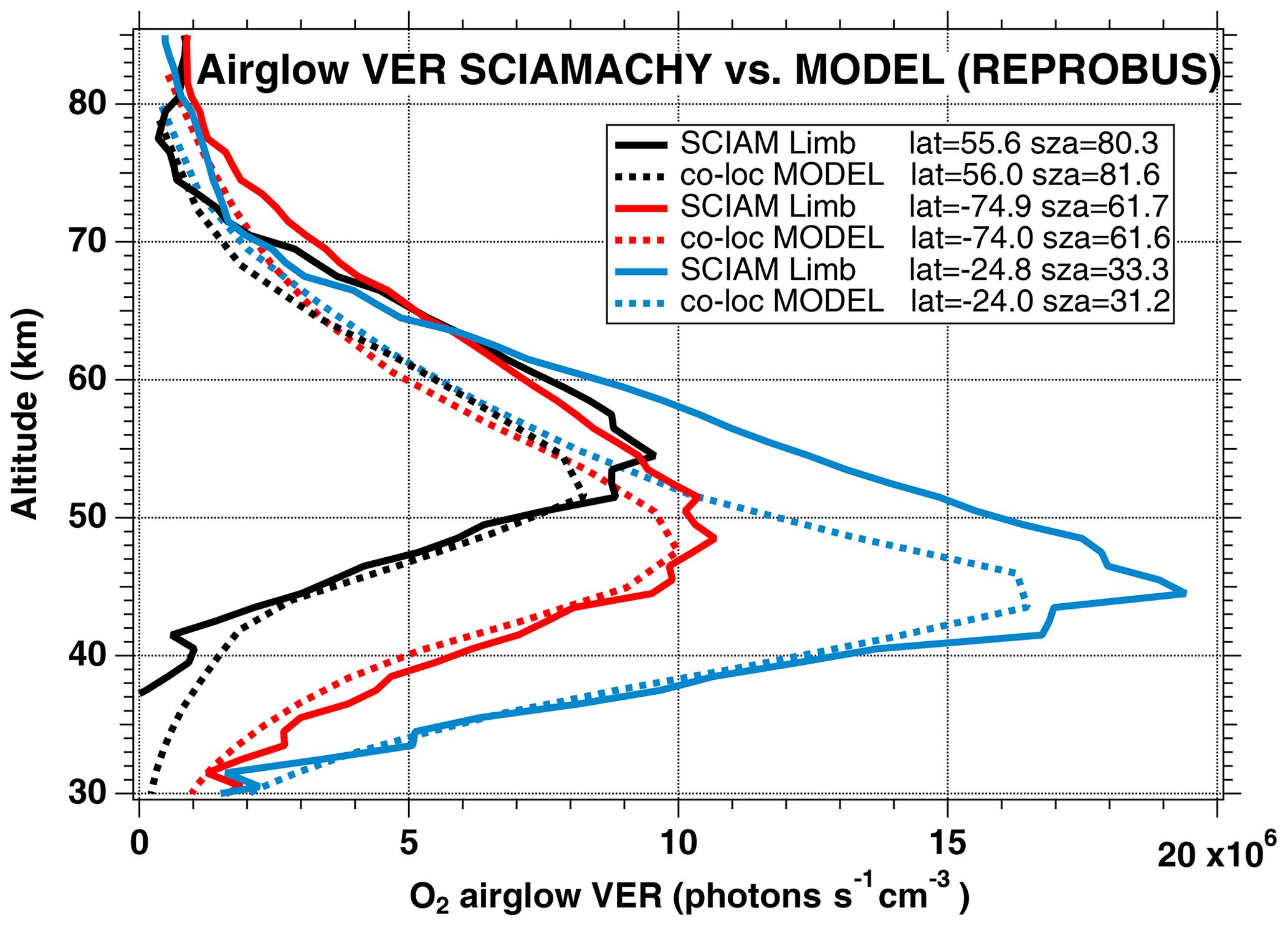
Figure 12 Comparison of SCIAMACHY and REPROBUS airglow VER profiles for 3 January 2007. Three profiles were drawn at SZAs of about 30, 60, and 80^∘, indicated in the legend. The SCIAMACHY profiles are plotted as solid lines and the geolocated REPROBUS profiles are plotted as dashed lines.

The same type of comparison is presented in Fig. 13a for a full set of SCIAMACHY limb observations obtained during the first 3 d of January 2007 but still selecting the SZA of tangent points in slices around 30, 60, and 80^∘, with a different colour for each SZA slice. The number of profiles were 66, 28, and 29, respectively, for slices around 30, 60, and 80^∘. Solid lines are the VER retrieved from SCIAMACHY, while dashed lines are calculated by the REPROBUS/airglow model. Only the data collected in the Southern Hemisphere are presented here. Figure 13b represents the relative difference $(\text{SCIAMACHY}-\text{Model})/\text{Model}$. Focusing our attention to the altitude range of 40–70 km where most of the emission occurs, it seems that the relative difference behaviour with altitude is identical for SZA of 80 and 60^∘ (green and blue curves) with a peak of discrepancy (about 30 % more observed emissivity) at 67 km, while for SZA around 30^∘ the peak of discrepancy is even larger (about 45 % more observed emissivity) but at a lower altitude ∼58 km. In Appendix C, we compare the ozone profile calculated by REPROBUS with ozone measurements taken by GOMOS on Envisat during the same period of time (year 2007). In short, this comparison suggests that at least one part of the airglow discrepancy is due to a deficit in the ozone predicted by REPROBUS (up to 15 %) in the range of 40–70 km (Fig. D3).

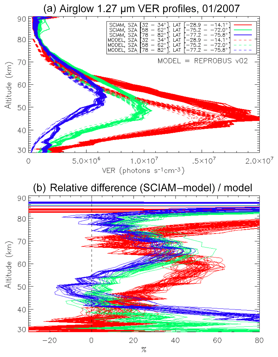
Figure 13 (a) Comparisons of all SCIAMACHY and REPROBUS airglow VER profiles for the first 3 d of January 2007 in three SZA domains: SZAs of 32–34^∘ (red curves), SZAs of 58–62^∘ (green curves), and SZAs of 78–82^∘ (blue curves). Only profiles from the Southern Hemisphere were selected. (b) For each profile, relative difference ($\text{SCIAMACHY}-\text{REPROBUS})/\text{REPROBUS}$ is shown.

Another possible reason for the discrepancy in airglow vertical profiles between our model and SCIAMACHY observations would be the radiometric calibration of SCIAMACHY in this airglow band. For the time being, we reject this hypothesis for two reasons. The first is that the radiometry of SCIAMACHY has been compared to other instruments with observation of deep convective clouds (DCCs) found in the tropics. A good agreement is found around 1300 nm when compared to MODIS and Hyperion hyperspectral sensor (Morstad et al., 2012). The second reason is that the onion-peel inversion scheme that we have designed to derive VER vertical profiles is a linear one. Therefore, changing the calibration of SCIAMACHY by a scaling factor would also change the VER profile by the same factor, while we see that the VER discrepancies are changing with altitude.

5 The MicroCarb mission

In the domain of Earth observations and GHG monitoring, CNES (Centre National d'Etudes Spatiales) has developed the MicroCarb mission, a space observatory dedicated to CO₂ monitoring. As a result of the studies conducted since 2016 by CNES concerning the use of the 1.27 µm O₂ band reported in the present paper, it was decided to incorporate in the instrument the 1.27 µm O₂ band as band B4.

The MicroCarb mission builds on a high spectral resolution infrared grating spectrometer aboard a microsatellite. The satellite platform is an enhanced version of the Myriade family. The total mass of the satellite including payload is 170 kg for a power of 100 W. MicroCarb will be launched in 2021 on an 11:30 h ascending node or alternately 13:30 h descending node heliosynchronous orbit (to be decided later).

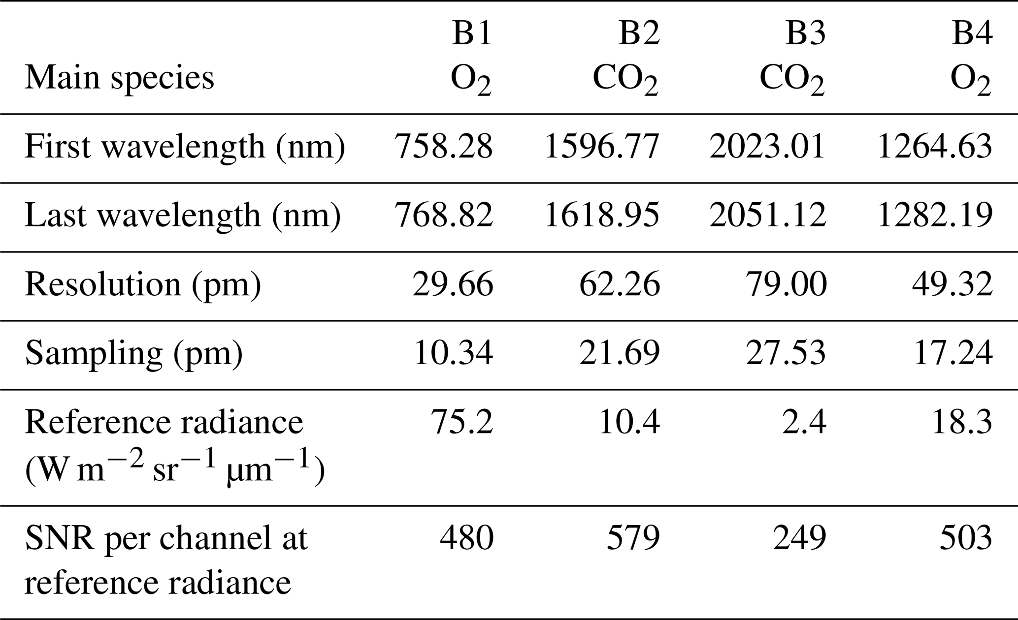
The MicroCarb data consist of the measurement in four spectral bands of the solar irradiance reflected by the surface and partially absorbed by atmospheric gases. Two bands are dedicated to the measurement of CO₂ around 1.60 µm (weak CO₂ B2) and 2.04 µm (strong CO₂ B3). Two spectral bands are dedicated to O₂ around 0.76 µm (strong O₂ B1) and 1.27 µm (weak O₂ B4). Figure 14 illustrates typical radiances in the four MicroCarb bands and Table 1 gives the main properties of the MicroCarb bands. The mechanical implementation on a microsatellite is enabled by a very compact design of the instrument, having a unique telescope, one slit per band, a unique grating and a unique Sofradir Next Generation Panchromatic 1024×1024 pixel detector for the four bands (Pasternak et al., 2016).

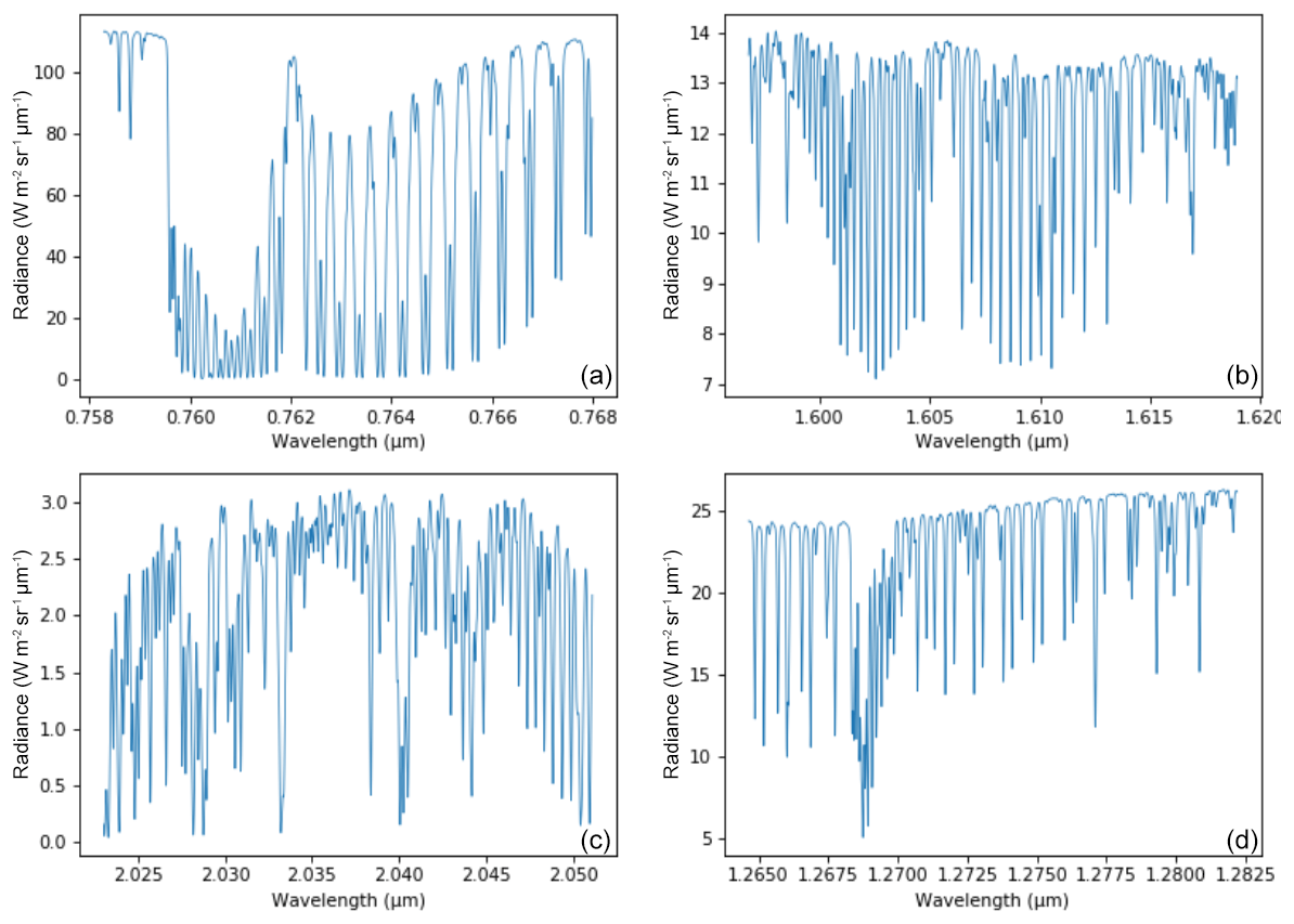
Figure 14 Example of MicroCarb simulated spectra of the strong O₂ band (B1) (a), the weak O₂ band (B2) (b), the strong O₂ band (B3) (c), and the weak O₂ band (B4) (d).

6 Disentangling O₂^* airglow from O₂ absorption in nadir-viewing spectra

6.1 Overview

With the theoretical shape of the O₂^* dayglow emission spectrum (Appendix A) and a selected VER vertical profile (e.g. Fig. D1), it is possible to construct a synthetic spectrum of the dayglow in absolute radiance units at the native spectral resolution of LBLRTM (several 10⁵), which may be degraded to any spectral resolution to simulate various instruments. For a given surface albedo and SZA, the radiance of solar radiation scattered by the surface modified by O₂ absorption may also be computed, using LBLRTM. Adding both spectra is a simulation of what will be seen by a nadir-viewing instrument (in the case of no aerosols) in the region around 1.27 µm, as shown in Fig. 15 for two cases with different albedos and SZA, where the two spectra are separated. The contribution of atmospheric Rayleigh scattering is small at this wavelength and ignored in this exercise.

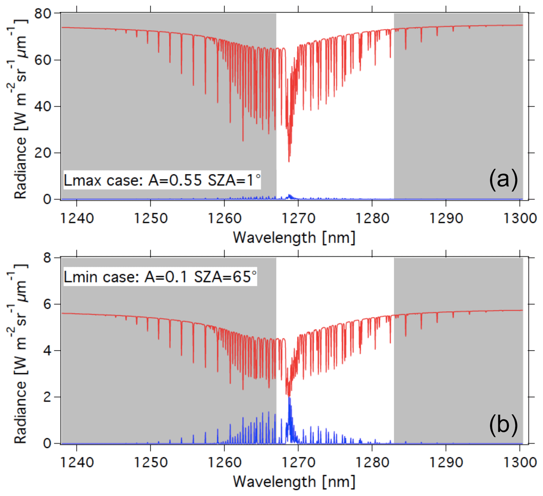
Figure 15 Airglow (blue) and scattered sunlight (red) absolute intensities and radiances (in W m⁻² sr⁻¹ µm⁻¹) for two cases: (a) high albedo (A=0.55) and almost sub-solar SZA of 1^∘ (referred to as the Lmax case (maximum luminance for instrument SNR estimates) and (b) low albedo (A=0.1) and high SZA of 65^∘ (referred as the Lmin case for SNR estimates for minimum luminance). The depression on the continuum of reflected sunlight is due to the O₂ CIA (now included in HITRAN 2016; Gordon et al., 2017). Water vapour absorption lines, which would be on the right part of the spectra, are not represented here. The white area corresponds to the MicroCarb wavelength coverage.

While the O₂^* emission spectrum (blue) is quite similar to the O₂ absorption spectrum imprinted on the albedo (red in Fig. 15b), there are five factors which make them different (as noted before), allowing their disentangling by spectral profile fitting:

• The transmission $T_{\mathrm{atm}}\left(\mathit{\tau }\right)=\exp (-\mathit{\tau })$ is not linear when τ>1, while the emission stays linear.

• Airglow lines are narrower than absorption lines (no pressure broadening at high altitude).

• The CIA affects only the O₂ absorption spectrum.

• As shown in Sect. 2 and Appendix A, the ratio of O₂^* emission to O₂ absorption is not a constant, but a continuous function of the wavenumber ν (in cm⁻¹).

• The temperatures near the surface and in the mesosphere are different, dictating different populations of rotational levels.

Basically a retrieval software tool allowing to determine from an observed spectrum simultaneously the albedo, the O₂ vertical column (or surface pressure P_surf, when the water vapour is ignored), and the O₂^* airglow intensity consists of two parts: a forward model to simulate what would be observed (depending on the parameters to be retrieved) and a scheme to minimize the χ² of the fit of the observed spectrum by the simulated spectrum (Levenberg–Marquardt).

For the present study, we have developed what we call the LATMOS breadboard, a software (in Igor Pro language version 8.0 from WaveMetrics) dedicated first to proof of concept for the use of the O₂ band at 1.27 µm in presence of O₂^* airglow contamination, and then we applied it to SCIAMACHY nadir observations, showing that when the albedo is weak, the O₂^* airglow intensity may be identified and its intensity actually measured, as a scaling factor of a synthetic airglow spectrum (see below in Sect. 6.2). We have also used the 4ARCTIC software to evaluate the performance of the particular MicroCarb instrument configuration (wavelength coverage and spectral resolution) and specified SNR as a function of spectral radiance of the nadir-viewing scenery (Sect. 6.3 and Appendix D).

6.2 Airglow inversion in nadir SCIAMACHY spectra

The possibility to extract 1.27 µm airglow information from nadir SCIAMACHY spectra is limited by the relatively low resolving power of this instrument (about 860). The intensity of the sunlight reflected by the surface and the atmosphere is in general much larger than the airglow in this spectral band. This is true above continents but above ocean, where the near infrared albedo is very low, it should be possible to extract the airglow when the sky is clear. We tested this possibility using the spectral inversion LATMOS breadboard, originally developed to test the possibility to determine the airglow intensity in the 1.27 µm O₂ band in the MicroCarb CO₂ mission.

6.2.1 Algorithm used in the LATMOS inversion breadboard

As said above, the spectrum observed by SCIAMACHY in the 1.27 µm band at nadir is the sum of the nadir solar flux reflected by the ground and the atmosphere, partly re-absorbed by atmospheric O₂, and the airglow O₂^* emission spectrum. For clear-sky conditions, if we neglect the reflection by the atmosphere, the reflected solar spectrum may be expressed as

$$\begin{array}{}\text{(8)}& I_{\mathrm{Nadir}}\left(\mathit{\lambda },\mathrm{sza}\right)=AF\left(\mathit{\lambda }\right){\displaystyle \frac{T_{\mathrm{atm}}^{\left(\mathrm{1}+\frac{\mathrm{1}}{\cos \left(\mathrm{sza}\right)}\right)}\cos \left(\mathrm{sza}\right)}{\mathit{\pi }}},\end{array}$$

where

• A is albedo (assuming a Lambert law (isotropic) reflectance);

• λ is wavelength;

• F(λ) is solar spectrum outside atmosphere;

• sza is solar zenith angle; and

• T_atm is one-way vertical atmospheric transmission.

The airglow spectrum is assumed to be proportional to the logarithm of the atmospheric O₂ transmission at high altitude multiplied by the emission to absorption ratio ε(λ)∕SS(λ) (Eq. 4) as explained in Appendix A. The relative intensity of the lines depends mainly on temperature. To take into account this dependency, we represent the airglow spectrum Ag(λ) as a linear combination of a warm spectrum Ag_warm(λ) and a cold spectrum Ag_cold(λ). These warm and cold spectra are computed using US standard atmosphere transmission tables from LBLRTM for nadir viewing around 50 km where the temperature is higher (270 K) and 70 km where the temperature is lower (217 K):

$$\begin{array}{}\text{(9)}& {\displaystyle }\begin{array}{rl}{\mathrm{Ag}}_{\mathrm{warm}}\left(\mathit{\lambda }\right)& \approx C_{\mathrm{norm}}\cdot \left[\mathrm{Ln}\right(T_{\mathrm{51}\mathrm{km}}\left(\mathit{\lambda }\right))\\ & -\mathrm{Ln}\left(T_{\mathrm{49}\mathrm{km}}\right(\mathit{\lambda }\left)\right]\cdot \left[\mathit{\epsilon }\right(\mathit{\lambda })/\text{SS}(\mathit{\lambda }\left)\right)]\end{array}\text{(10)}& {\displaystyle }\begin{array}{rl}{\mathrm{Ag}}_{\mathrm{cold}}\left(\mathit{\lambda }\right)& \approx C_{\mathrm{norm}}\cdot \left[\mathrm{Ln}\right(T_{\mathrm{71}\mathrm{km}}\left(\mathit{\lambda }\right))\\ & -\mathrm{Ln}\left(T_{\mathrm{69}\mathrm{km}}\right(\mathit{\lambda }\left)\right]\cdot \left[\mathit{\epsilon }\right(\mathit{\lambda }\left)\text{SS}\right(\mathit{\lambda }\left)\right],\end{array}\end{array}$$

where T_z(λ) is the transmission at wavelength λ from altitude z to the top of the atmosphere and C_norm a normalization constant determined in order that the integral of the spectrum is equal to the integral of a reference spectrum, and using Eqs. (A15) and (4).

A Levenberg–Marquardt (L–M) method is used to determine the parameters giving the best fit to SCIAMACHY spectra. The total column of O₂, assimilated to surface pressure, the airglow, the H₂O column and the albedo are inverted using the L–M converging scheme. As atmospheric transmission depends non-linearly on the O₂ column, its Jacobian is calculated at ground level from the difference in transmission between the ground and 1 km altitude.

The measured spectrum will therefore be expressed as

$$\begin{array}{}\text{(11)}& \begin{array}{rl}F\left(\mathit{\lambda }\right)& =K_{\mathrm{1}}\cdot \left[\left(\mathrm{1}-K_{\mathrm{2}}\right)\cdot I_{{\mathrm{Nadir}}_{\mathrm{0}\mathrm{km}}}\left(\mathit{\lambda }\right)+K_{\mathrm{2}}\cdot I_{{\mathrm{Nadir}}_{\mathrm{1}\mathrm{km}}}\left(\mathit{\lambda }\right)\right]\\ & \cdot T_{{\mathrm{H}}_{\mathrm{2}}\mathrm{O}}^{K\mathrm{5}}+K_{\mathrm{3}}\cdot {\mathrm{Ag}}_{\mathrm{warm}}\left(\mathit{\lambda }\right)+K_{\mathrm{4}}\cdot {\mathrm{Ag}}_{\mathrm{cold}}\left(\mathit{\lambda }\right),\end{array}\end{array}$$

where K₁ is the intensity of the reflected spectrum (proportional to the albedo); K₂ is the sensitivity of the reflected spectrum to surface pressure; K₃ is the warm component of the airglow spectrum; K₄ is the cold component of the airglow spectrum. $T_{{\mathrm{H}}_{\mathrm{2}}\mathrm{O}}$ is the atmospheric transmission of water vapour for a reference column of H₂O, and is elevated to the power K₅ to compute the transmission of another column of water vapour, where K₅ is the ratio of H₂O column ∕ reference column. There are some weak lines of H₂O in the area around the 1.27 µm band that must be accounted for when comparing forward simulations with real data. The coefficients K₁, K₂, K₃, K₄, K₅ can be imposed or left free in the L–M inversion. The measurement uncertainty in each spectel (spectral element) is assumed to be proportional to the square root of the signal.

6.2.2 Application to SCIAMACHY nadir-viewing observations: retrieval of O₂^* airglow intensity at 1.27 µm

The inversion scheme was applied to 3 d of SCIAMACHY nadir data above the ocean (1–3 April 2007). For the L–M inversion, SCIAMACHY nadir characteristics are taken from OSCAR https://www.wmo-sat.info/oscar/satellites (last access: 11 June 2020)

• Band 971–1773 nm

• Spectral resolution 1.48 nm (resolving power 858 at 1.27 µm)

• SNR 1500 at 25 W m⁻² sr⁻¹ µm⁻¹

The SNR is probably optimistic but it does not matter for the present study. The uncertainty is not calculated from the data SNR but estimated roughly from the dispersion of the airglow intensity results. The dispersion depends very much on the intensity of the backscattered solar flux as shown in Fig. 17, being high for large intensities and much smaller at lower levels.

Figure 16 shows two examples of similar SZA spectra (35–36^∘): one with a high radiance over a thick cloud cover and one with a low radiance on a clear day. In the case of high-reflected radiance (Fig. 16a), the 1.27 µm band is dominated by O₂ absorption, with the airglow filling only slightly the bottom of the lines. In the case of low reflected flux (Fig. 16b), the band is dominated by the airglow.

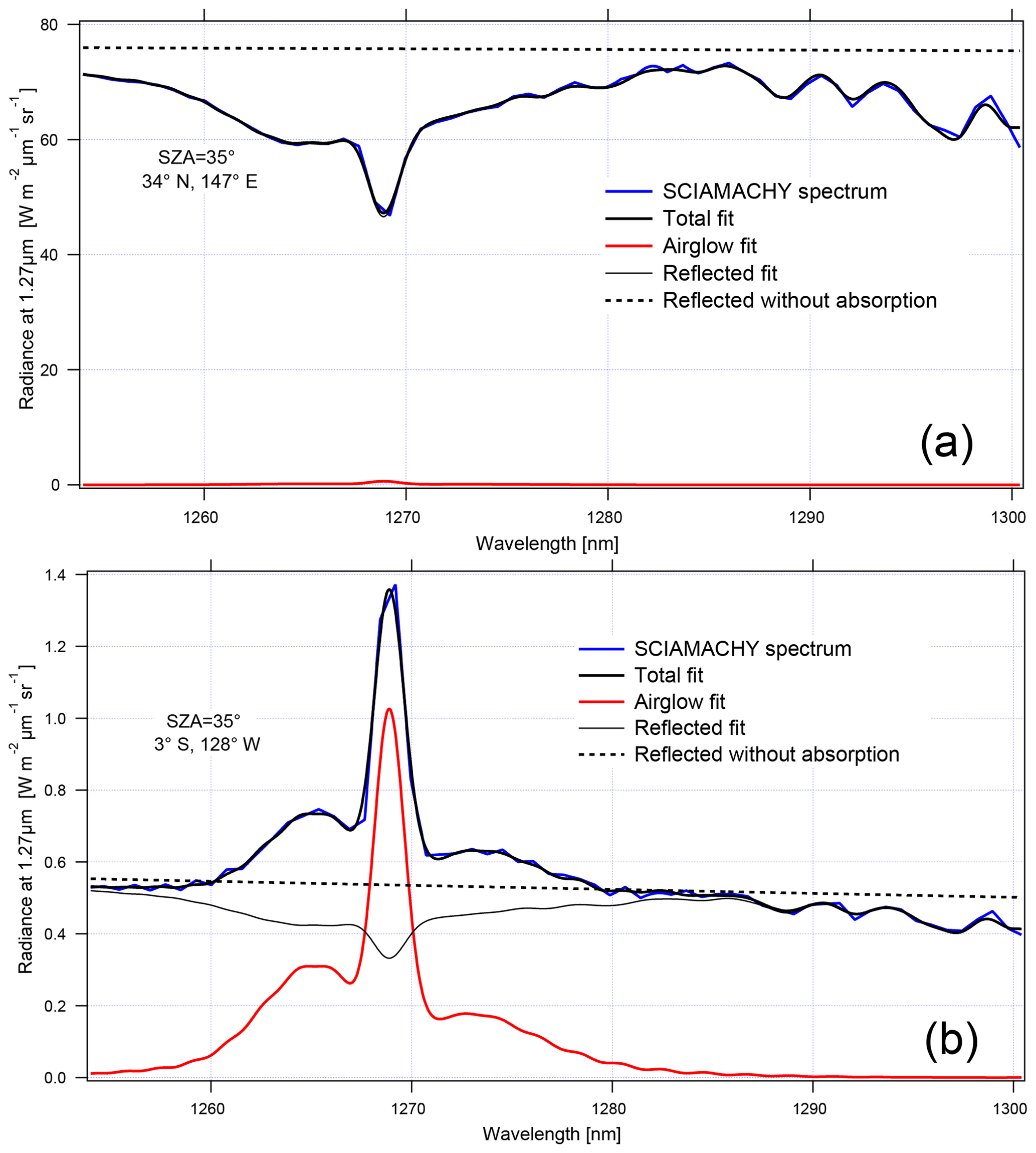
Figure 16 Two examples of SCIAMACHY spectra at nadir: (a) above thick clouds and (b) above clear ocean. The SCIAMACHY spectrum is in blue, fitted spectrum in thick black, determined airglow spectrum in red, fitted reflected spectrum in light black, and reflected spectrum without absorption in dotted black. The word “radiance” in the label axis indicates the spectral radiance or intensities.

In Fig. 17, it can be seen that when the reflected solar radiance is small, the values of the inverted airglow intensity are little dispersed. On the contrary, a very high dispersion is observed with a high-reflected radiance. It is concluded that airglow inversion is only possible at low reflected solar radiance, corresponding to situations above the ocean on a clear day or at a high SZA. For the rest of this study of SCIAMACHY nadir observations, we will limit the analysis to spectra with a reflected radiance lower than 5 W m⁻² sr⁻¹ µm⁻¹.

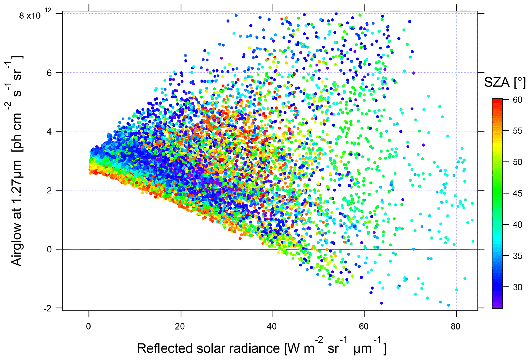
Figure 17 Intensity of the inverted airglow as a function of the reflected solar spectral radiance (in units of W m⁻² sr⁻¹ µm⁻¹). The points are coloured according to the SZA from blue to red from 27 to 60^∘.

In order to validate the airglow values inverted using nadir observations, we compare them to the values inverted using limb observations (Fig. 18). The latter are obtained by vertical inversion of the airglow profile observed at limb and integrated over the vertical column as described in Appendix B. The good agreement observed between the two methods gives us confidence in the results obtained with nadir observations. On the other hand, when the data are compared to our model, there is an underestimation of the nadir intensity of the airglow simulated by REPROBUS v02 of about 10 %–15 %. This underestimation had already been found for limb comparisons. The inverted airglow follows the same SZA dependence as that simulated by REPROBUS. It can be noticed that for SZA >90^∘, the airglow values at nadir are divided into two families of different intensity. Figure 19 shows these values with distinction between morning and evening data. The higher values in the evening than in the morning are due to the long lifetime of O₂(a¹Δ_g), greater than 1 h in the absence of quenching in the high mesosphere. REPROBUS cannot reproduce this morning–evening difference, the concentration of O₂(a¹Δ_g) being calculated by assuming the photochemical equilibrium.

Figure 18 Airglow intensity at nadir according to the SZA for the month of April 2007: in red are SCIAMACHY measurements at nadir with a reflected solar spectral radiance <5 W m⁻² sr⁻¹ µm⁻¹; in blue are nadir intensities retrieved from SCIAMACHY measurements at the limb; in black are simulations with REPROBUS v02. The airglow intensity at its maximum reaches 3.2×10¹² photons cm⁻² s⁻¹ sr⁻¹, which corresponds to 5 mW m⁻² sr⁻¹ (spread over a few nanometres' wavelength), to be compared to a solar backscattered luminance (radiance) of ∼5 to 70 W m⁻² sr⁻¹ µm⁻¹ (see Fig. 16).

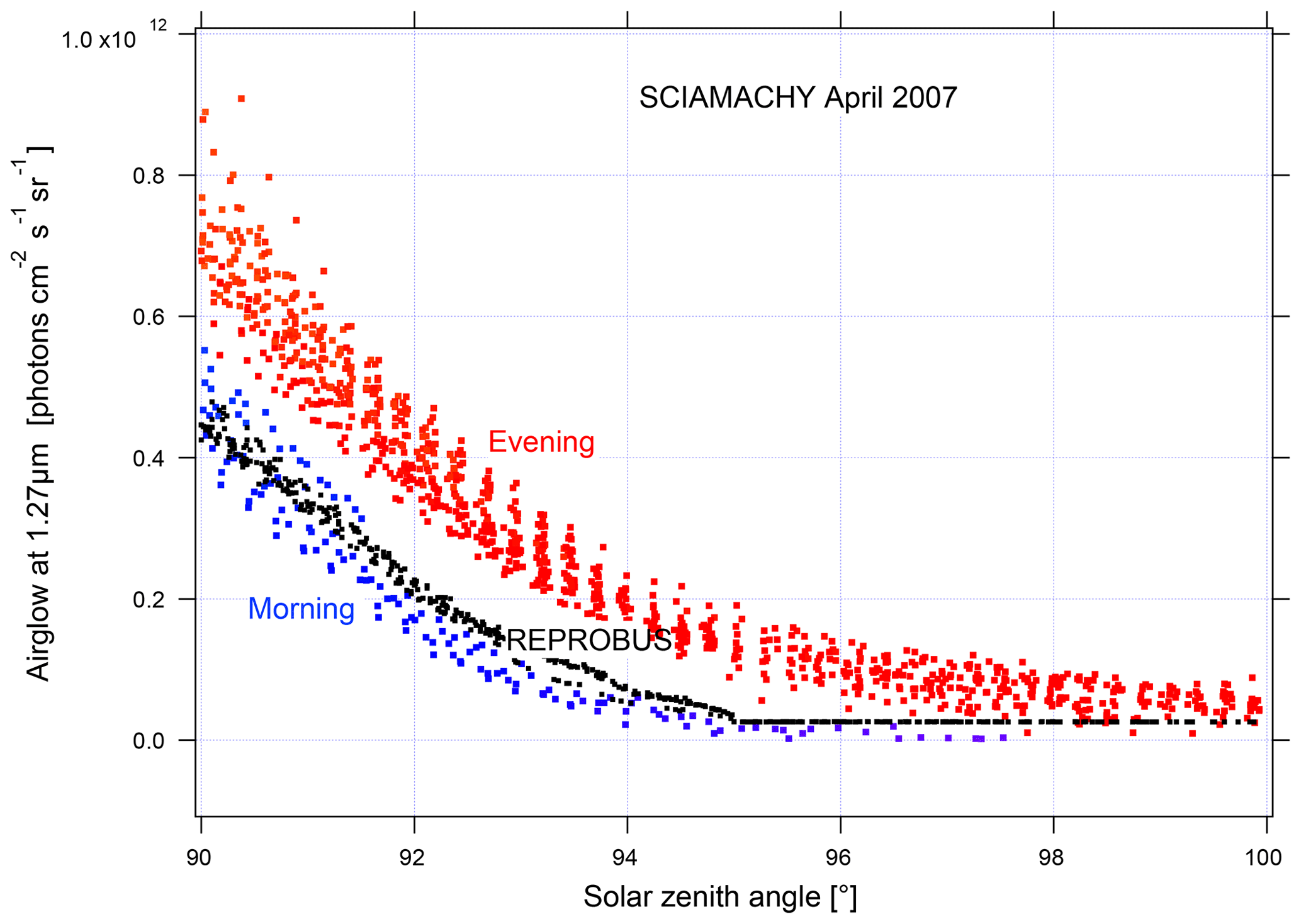
Figure 19 Airglow nadir intensity versus SZA for SZA >90^∘; SCIAMACHY measurements are in red during the evening and in blue during the morning; REPROBUS v02 simulations are in black. The observed difference between morning and evening values is due to the long lifetime of O₂(a¹Δ_g).

In order to evaluate the underestimation of the airglow by REPROBUS, a linear regression is performed between the SCIAMACHY measurements with nadir and the nearest REPROBUS values in time and position (Fig. 20). The slope of the regression is 1.13. SCIAMACHY therefore sees on average 13 % more airglow than estimated with REPROBUS. The regression line does not go through the origin but to 2×10¹¹ photons cm⁻² s⁻¹ sr⁻¹. This can be attributed to not taking into account in REPROBUS the airglow above 80 km that is present both day and night.

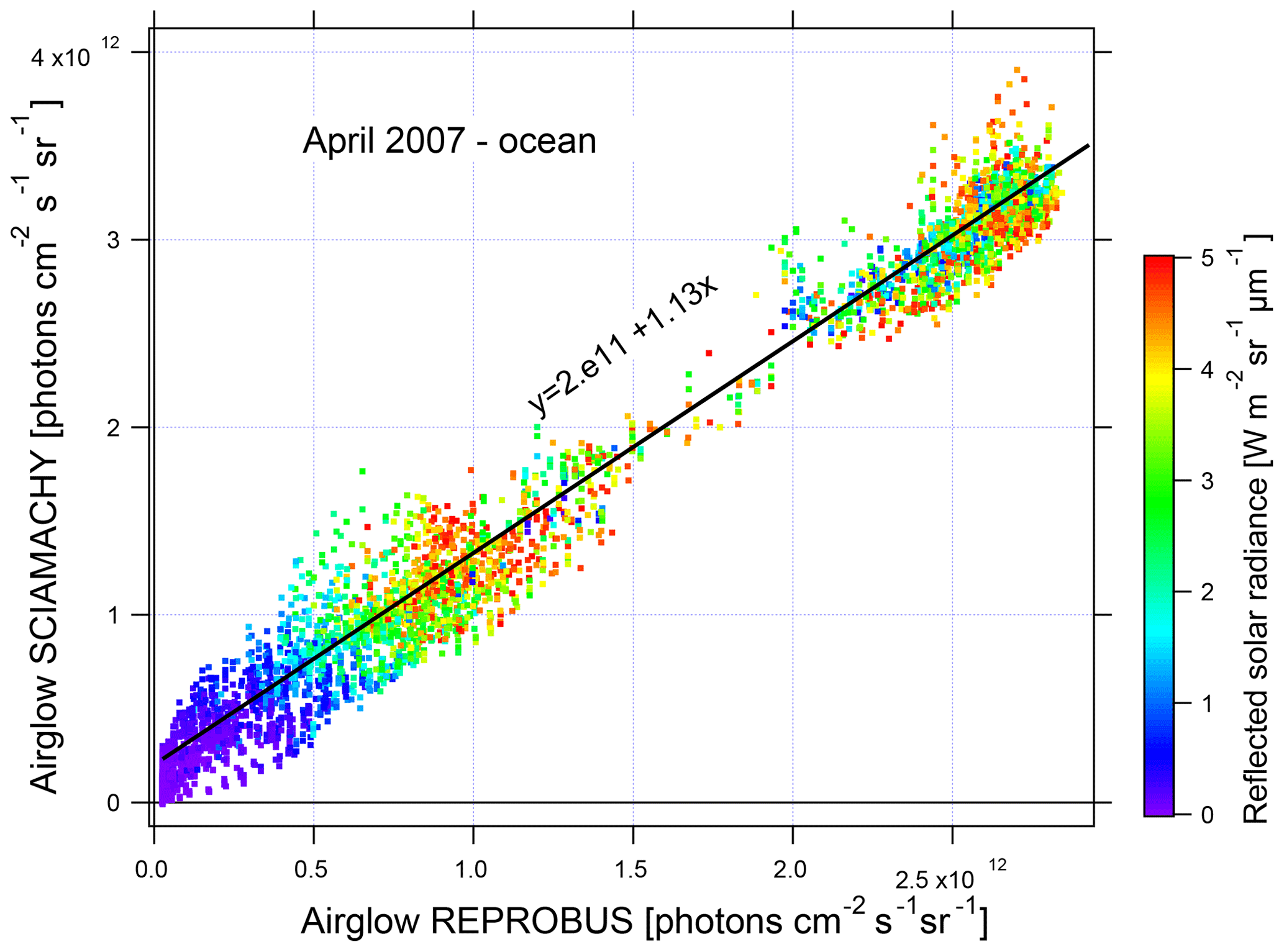
Figure 20 Nadir airglow SCIAMACHY observed intensities versus REPROBUS v02 simulation (same units on both axes, photons cm⁻² s⁻¹ sr⁻¹). The dots are coloured according to the reflected solar radiance from 0 in blue to 5 W m⁻² sr⁻¹ in red. Linear regression of the correlation is in black. Airglow intensity values are expressed in ph cm⁻² s⁻¹ sr⁻¹.

We have demonstrated that, despite the moderate resolving power of SCIAMACHY (∼860 against 25 000 for the future MicroCarb mission), it is possible to extract the O₂ airglow at 1.27 µm in nadir spectra provided that the spectra are selected above the sea with a low reflected solar flux (clear-sky conditions). The inverted airglow is on average 13 % higher than that simulated by REPROBUS v02, in agreement with REPROBUS – SCIAMACHY comparisons at limb (Sect. 4.2.1). The inverted airglow follows the same SZA dependency as that simulated by REPROBUS except at twilight where the morning–evening difference is not reproduced by REPROBUS which assumes photochemical equilibrium. Sun et al. (2018) had concluded that it is not possible to extract nadir airglow from SCIAMACHY measurements. We have shown on the contrary that this is possible if we select the low flux spectra reflected over the ocean in clear weather.

With MicroCarb data and its higher resolving power, one will be able around coastal zones to compare the O₂^* airglow intensity measured above the sea and above the ground, just nearby. They should be very similar, if the spatial characteristic lengths of intensity variations are as large as found by REPROBUS model, larger than the 2×2^∘ REPROBUS resolution. This comparison would provide an important “sanity check” of the retrieval of O₂ column, from which is derived Psurf assuming that the column of dry air is strictly proportional to the O₂ column, and adding the pressure due to the column of H₂O. Psurf is explicitly an element of the state vector to be retrieved in GHG retrievals.

Following an interesting suggestion of one of the anonymous referees, we have tried to estimate the small-scale horizontal variations of O₂^* airglow from nadir-viewing SCIAMACHY data that could be due to gravity waves and are not represented in REPROBUS CTM. This is not an easy task using the relatively low spectral resolution of SCIAMACHY data. At this resolution, spectral features in airglow and O₂ absorption spectra are highly correlated and the estimation of airglow is accurate only for very low values of reflected solar flux as illustrated in Fig. 17, where a large dispersion of airglow is observed for high values of reflected solar radiance. There are not enough observations reaching a low level of solar flux to plot maps of airglow. In spite of these limitations, we made an attempt to estimate at least an upper limit for the small-scale variations of airglow. We selected all pairs of nadir observations with reflected solar flux <2 mW m⁻² nm⁻¹ sr⁻¹, solar zenith angle <60^∘ and distance <110 km. With these strong criteria, only 1 % of the observations were selected. The average relative difference in airglow intensity between the pairs of observations was equal to 1.0 %. We consider this value as an upper limit of the impact of gravity wave perturbation in airglow intensity. At this level, the impact on the retrieval of O₂ column (and Psurf) and $X_{{\mathrm{CO}}_{\mathrm{2}}}$ will be very limited.

6.3 Surface pressure retrieval on simulated nadir spectra with MicroCarb parameters

With the instrumental characteristics of MicroCarb (Sect. 5), we have explored the accuracy of surface pressure retrieval in presence of the contaminating O₂^* airglow, using the dedicated 4ARTIC v4.2 software. The details of the exercise, done with several variants but using only the band B4 (1.27 µm) are described in Appendix D, with a brief summary below.

The requirements specified for the MicroCarb mission for Psurf accuracy calls for a bias <0.1 hPa, and a random error <1 hPa. We found out that, if the O₂^* airglow is ignored in the forward model used for the retrieval, the bias on Psurf depends on the back scattered solar light, but may amount to about 60 hPa (for a mean radiance with albedo of 0.2). Putting the O₂^* airglow in the forward model, we found out that, if the shape of the O₂^* airglow spectrum is perfectly known, a very small bias is achieved (−0.002 hPa), with a random error of 0.88 hPa. In reality, the shape in nadir viewing may depend on the temperature of the atmosphere below, at the altitude of emission. We found out that we could find a good fit to the simulated data by a linear combination of two airglow models, at two different temperatures (similarly as in Sect. 6.2.1). In this case, the random error was 0.88 hPa (compliant to requirements), and a bias of −0.11 hPa, marginally non-compliant with the <0.1 hPa bias requirement (Table 2 in Appendix D).

Therefore, we have demonstrated with these simulations that with the spectral resolving power of MicroCarb (25 000), and only using the O₂ IR band B4 at 1.27 µm, we may retrieve Psurf (or similarly the O₂ vertical column of dry air) with an accuracy almost compliant with the MicroCarb requirements. Other tests were also made with 4ARTIC, by using simultaneously both O₂ bands B1 (0.76 µm) and B4 (1.27 µm) of MicroCarb. Of course, it improves very much the retrieval accuracy, but since we are investigating the use of the B4 band because band B1 is suspected to present some problems, we do not show the results here. It will be particularly interesting to investigate the improvement of using the B4 band, in addition to the B1, in the presence of aerosols. This is way beyond the scope of the present study. However, the capability to disentangle the spectrum of the O₂^* emission from the O₂ IR absorption with their fine structure should not depend very much on the presence of aerosols, in view of their slowly varying spectral signature with wavelength.

7 Conclusions

In this paper, we have reported the results of a 3 years (2016–2018) scientific research effort to revisit the use of the O₂ absorption band at 1.27 µm in the problem of GHG retrieval from space observations of the detailed spectrum of the solar radiation scattered by aerosols, atmosphere and surface. It is widely recognized that this 1.27 µm band being nearer in wavelength to the CO₂ bands at 1.6 and 2.0 µm, it should be in principle less uncertain to “transport” aerosols optical properties (wavelength dependent) from this O₂ band to the CO₂ bands, than from the O₂ A band at 0.76 µm. However, the O₂ absorption band at 1.27 µm is contaminated by a strong airglow emission, presenting a similar spectral structure. This airglow is mainly due to the spontaneous relaxation of excited oxygen O₂(a¹Δ_g) that is formed in the photolysis of ozone.

7.1 Nadir O₂^* airglow intensity

As a first approach, we needed to have an idea of the absolute amount of O₂^* airglow radiance, in order to compare to the expected solar scattered radiances in nadir viewing which are well documented. We could not use the SCIAMACHY nadir observations around 1.27 µm for this purpose, since they are mixed with solar scattered radiation from the surface. Therefore, we used the limb-viewing observations of SCIAMACHY in this band, which are not contaminated by atmosphere/aerosols scattering of solar radiation when looking above ∼30 km altitude. We have designed a method to retrieve the vertical profile of the O₂^* VER from a limb scan of SCIAMACHY, taking into account the re-absorption of O₂ along each LOS. A “fictitious” nadir-viewing intensity from SCIAMACHY could therefore be derived by vertical integration of the VER. When extracting the data for various periods of the year, it was found that the major factor governing this O₂^* airglow intensity was the Solar Zenith Angle, with little variability otherwise.

In parallel, we have conducted a major effort to model the intensity of the O₂^* airglow emission, as an offline extension of the CTM REPROBUS model providing the ozone field within the ECMWF meteorological field. We found the same overall behaviour with SZA and some weak seasonal dependence. A systematic comparison of 12 833 limb-scans acquired by SCIAMACHY in 2007 and corresponding fictitious nadir-viewing intensities with the prediction of our model (and also VER vertical profiles) indicates an overall good agreement, although with a deficit of about 15 % in the modelled intensity with regard to the SCIAMACHY intensity. For the time being, we assign this deficit to be due at least partially (but possibly not totally) to an ozone deficit in the REPROBUS model, as suggested by comparisons with dayside GOMOS ozone vertical profiles obtained by the technique of star occultation (not sensitive to an absolute calibration).

In summary, we have found that the intensity of the O₂^* airglow is well behaved (with a weak horizontal variability), and quite predictable, with a dispersion of probably only a few per cent around a climatological average. Also, it should be almost as good as the ozone field in CTM models which are run with the actual meteorological fields like ECMWF. Therefore, one could imagine that a GHG nadir-viewing observation in the O₂ band could be corrected by subtraction of a model of the O₂^* airglow to get the pure nadir solar scattered intensity (on which is imprinted the O₂ absorption that we are analysing to get the O₂ column). However, the degree of accuracy that is needed for the determination of Psurf for useful measurements of GHG gases is very large, about ∼0.1 hPa for the bias and 1 hPa for random error. According to our simulations, and if the airglow is ignored in the inversion but subtracted from a model, this airglow intensity model would have to be accurate to ∼1.5 % (for a mean radiance with albedo of 0.2) to achieve the 1 hPa random error. Therefore, in most cases, it is insufficient to rely entirely on a model to predict the actual airglow intensity to be subtracted from an observation. We need to disentangle in the observed spectrum itself the contribution of the airglow and the contribution of the solar scattered radiation. For this, we will rely on the fact that the spectrum shape of the O₂^* airglow is different from the O₂ absorption spectrum. Still, if the high horizontal smoothness of the intensity predicted by the model is confirmed by the MicroCarb observations, it will help the retrieval. With the limited disentangling capabilities of SCIAMACHY, we have shown that the data indicate fluctuations (at constant SZA) smaller than 1 %, with a negligible impact on the $X_{{\mathrm{CO}}_{\mathrm{2}}}$ retrieval accuracy.

7.2 Spectral shape of the O₂^* airglow

It is clear that if the dayglow spectrum of O₂^* were strictly identical to the O₂ absorption spectrum, it would be impossible to disentangle one from the other, and one would have to subtract blindly a model of the airglow emission from the observed spectrum, with an associated uncertainty.

While all the transitions of the O₂ 1.27 µm do exist in both the absorption spectrum and in the O₂^* airglow emission spectrum, the resulting spectra in a nadir-viewing geometry are different for two reasons and under three aspects.

First, the emission happens at high altitude and low air densities, while the absorption happens in the dense, lower atmosphere. Therefore, each absorption line is broadened by collisions, as shown in Fig. 2. Also, while for the shape of the airglow emission, all the spectral lines are proportional to each other, on the contrary the radiance factor ($=\mathit{\pi }\mathrm{B}/\mathrm{solar}$ flux cos(SZA), B brightness) is modulated by the O₂ transmittance spectrum (Tr(τ) $=\exp (-\mathit{\tau }))$ which is not linear for the strong lines with large τ. Finally, there is the CIA effect producing a broadband absorption (Fig. 15), which is totally negligible in the upper atmosphere where emission takes place.

Second, for the same line of the electronic transition described by the rotational states J^′ (upper level), J^′′ (lower level), the relative populations are dictated by the numbers J^′ (relevant for emission) and J^′′ (relevant for absorption). For the P and R branches ($\mathrm{\Delta }J=\pm \mathrm{1}$) with $J^{\prime }\ne J^{\prime \prime }$, the relative populations for emission and absorption are therefore different.

We have computed the theoretical shape of the dayglow spectrum from the Einstein coefficients A₂₁ of spontaneous emission from data contained in the HITRAN database. It depends on the temperature of the atmosphere at the place of emission (rotational relative populations). We have compared our theoretical spectra degraded to the resolving power of SCIAMACHY (∼860) with limb observations of SCIAMACHY and found an overall excellent agreement, validating our theoretical approach of the airglow spectrum. This allowed performing some simulation exercises (see below in Sect. 7.3) with good confidence about their ability to represent reality, showing that with the resolving power of 25 000 of the MicroCarb instrument, it is indeed possible to disentangle the airglow emission from the O₂ absorption in the O₂ band at 1.27 µm. We note that the broad CIA band would not require such a high spectral resolution to be useful for the disentangling.

7.3 Simulation of Psurf retrievals

Simulation exercises performed with the 4ARCTIC software (Sect. 6.3 and Appendix D) have demonstrated that with the resolving power of MicroCarb (25 000), and only using the O₂ IR band B4 at 1.27 µm, we may retrieve Psurf (or similarly the O₂ vertical column of dry air) with an accuracy (bias of −0.11 hPa) almost compliant with the strong MicroCarb requirements: bias <0.1 hPa. The use of the B1 band (0.76 µm), in addition to the B4 band, will most likely yield a better understanding of the behaviour of this band B1 which at present is not fully understood. Once better understood, it will certainly improve the accuracy of the Psurf MicroCarb retrieval by constraining further the aerosols optical properties. One may even hope that such a new knowledge could be used for an improved retrieval of other GHG missions using only the A band.

One may wonder if the 25 000 resolving power is absolutely necessary to disentangle the O₂^* emission from the O₂ absorption at 1.27 µm with sufficient accuracy for GHG retrievals. Sun et al. (2018) have explored spectral resolving power down to ∼4200, and found (their Fig. 4) an accuracy on the O₂ column of ∼0.35 % for an SNR of ∼500 and a spectral resolving power of 5700, which would result on an error of 1.4 ppm for $X_{{\mathrm{CO}}_{\mathrm{2}}}$ (0.35 %×410 ppm), marginally insufficient. Their whole analysis was done with already accounting for the CIA O₂ absorption, whose broad size and smooth pattern is insensitive to spectral resolving power (Fig. 15). On the other hand, as can be seen in Fig. 15 with the same number of spectels as MicroCarb and a coarser spectral resolution (and sampling), the whole O₂ band would be measured and would possibly allow to better constrain the CIA absorption and O₂ column retrieval. The larger spectral sampling gives additional photons per spectel, which may be traded off for an increased spatial resolution. However, the high resolving power of MicroCarb is an asset for the exact knowledge of the instrumental spectral function which is also important for the retrieval accuracy.

On the other hand, with our Igor–software breadboard tool, we have shown that with the SCIAMACHY spectral resolving power (∼860), it was possible to determine the intensity of the O₂^* airglow over oceans (low albedo) but not to disentangle it and retrieve the CO₂ column, whatever the albedo, with a useful enough accuracy. We suggest though, on the basis of our analysis and the results of Sun et al. (2018), that when CIA is taken into account, a spectral resolving power of about 5000 and a high SNR could possibly yield a sufficiently good accuracy on the Psurf retrieval in the O₂ band at 1.27 µm, and could improve the treatment of aerosols and their wavelength dependent optical properties, being nearer the CO₂ bands, for a better $X_{{\mathrm{CO}}_{\mathrm{2}}}$ retrieval. The CO₂ Mission (space mission CO₂-M) is sponsored by European Community, and developed and operated by ESA, as a space segment for the monitoring of CO₂ anthropogenic emissions, with potentially a series of three operational spacecraft on Sun-synchronous orbits. The present typical baseline optical design of the CO₂-M has a spectral resolving power of about 6300 at 0.76 µm, and 5400 for the weak CO₂ channel at 1.60 µm. There is no channel for the O₂ band at 1.27 µm but it can be imagined by interpolation that a new channel for this band derived from the baseline design would have a resolving power of about 5750. Based on the discussion in the previous paragraph and on the whole present study, we advocate for the inclusion in the design of CO₂-M instrument of a channel at 1.27 µm.

TANSO-GOSAT is a Fourier transform spectrometer dedicated to GHG monitoring on JAXA GOSAT space platform. TANSO-GOSAT2 was launched in October 2018 and use bands at 0.76 (for O₂), 1.60 µm weak CO₂ band and 2.0 µm (strong CO₂ band). We advocate for the inclusion of an additional channel dedicated to the measurement of the O₂ band at 1.27 µm in the design of future Thermal And Near infrared Sensor for carbon Observation (TANSO) instruments, as well as for the Chinese family of TanSat following the TanSat-1 already collecting data.

Finally, we have mentioned in Appendix E other cases where an airglow emission could contaminate nadir-viewing observations from space analysing scattered sunlight, since the LOS goes across all the airglow layers (Fig. 1). We listed a few commonly used absorption bands and their potential contamination by airglow: the O₂ molecule and the band A emission, CO₂, H₂O, CH₄ and CO molecules where fluorescence induced by solar light could be a source of contamination. These situations would deserve more detailed calculations to estimate the impact on their column abundance retrievals.

Appendix A: Modelling the airglow emission of O₂^* excited molecule

A1 Spectroscopy: the various electronic states of the O₂ molecule

Figure A1 (from Khomich et al., 2008) presents the various electronic states of the di-oxygen molecule O₂ and the names of the transitions between them. The O₂ molecule, being composed of two identical atoms, is said to be homopolar. The fundamental state $X^{\mathrm{3}}{\mathrm{\Sigma }}_g^{-}$ is put at a reference energy level of 0. The number 3 indicates a triplet state, which may be decomposed in three sub-states with very nearby energies. The descending arrows in Fig. A1 indicate transitions to a lower level, corresponding to the emission of one photon. The reverse process corresponds to the absorption of one photon. We describe briefly below three of the transitions indicated in Fig. A1 which are the most relevant to GHGs, since O₂ is used as a reference to determine the mixing ratio of CO₂. We can make use of the energy/wavelength conversion:

$$\begin{array}{}\text{(A1)}& E\left(ev\right)=h\mathit{\nu }={\displaystyle \frac{hc}{\mathit{\lambda }}}={\displaystyle \frac{\mathrm{1242.26}}{\mathit{\lambda }\left(\text{nm}\right)}}.\end{array}$$

1. The Schumann–Runge band is in the far UV. The UV solar flux dissociates also O₂ molecules, producing O atoms, which may recombine with O₂ to form O₃, which absorbs in the nearer end of the UV spectrum. All together, O₂ and O₃ are protecting life (and DNA molecules) from harmful solar UV.

2. The “atmospheric” band is the transition ($b^{\mathrm{1}}{\mathrm{\Sigma }}_g^{+}\to X^{\mathrm{3}}{\mathrm{\Sigma }}_g^{-}$), around 760 nm, also called the A band from Fraunhofer's early nomenclature, or “atmospheric band”, heavily used in GHG studies.

3. The “infrared atmospheric” band is the transition ($a^{\mathrm{1}}{\mathrm{\Delta }}_g\to X^{\mathrm{3}}{\mathrm{\Sigma }}_g^{-})$, around 1270 or 1.27 µm in the near infrared, sometimes called the O₂ IR band, or ¹Delta band (according to Gordon et al., 2010). This band is the subject of the present study.

Because the O₂ molecule is homopolar, it has no electric dipolar moment and in principle electronic transitions are forbidden. The electronic transitions can only happen thanks to the existence of a magnetic dipole moment (M1) and/or a quadrupolar electric moment (E2). As a consequence, spontaneous transitions from a given electronic state down to the fundamental state $X^{\mathrm{3}}{\mathrm{\Sigma }}_g^{-}$ are unlikely; therefore, the lifetime of such a state is rather long: 13 s for the atmospheric A band at 760 nm, transition ($b^{\mathrm{1}}{\mathrm{\Sigma }}_g^{+}\to X^{\mathrm{3}}{\mathrm{\Sigma }}_g^{-}$) (Mlynczak and Solomon, 1993) and 75 min for the O₂ IR band at 1.27 µm, transition ($a^{\mathrm{1}}{\mathrm{\Delta }}_g\to X^{\mathrm{3}}{\mathrm{\Sigma }}_g^{-}$) (Lafferty et al., 1998). Therefore, the O₂ molecule excited at level a¹Δ_g (often represented by O₂^* or O₂(¹Δ) in this paper) which results from ozone photo-dissociation has plenty of time to reach thermal equilibrium with ambient gas, and the various states of vibration rotation will be populated according to a Boltzmann law (therefore, depending on the local temperature T) modulated by the rotation quantum number J, with a statistical weight 2J+1 as described later below.

For the O₂ IR band at 1.27 µm, the transition ($a^{\mathrm{1}}{\mathrm{\Delta }}_g\to X^{\mathrm{3}}{\mathrm{\Sigma }}_g^{-}$) is mainly due to a magnetic dipole (M1). There is, however, also a system of absorption lines due to the electric quadrupole: (E2), identified for the first time both in atmospheric absorption spectra (looking at the Sun) and in laboratory experiments (Gordon et al., 2010). The overall absolute strength of this (E2) system is about 215 times weaker than the (M1) system (Gordon et al., 2010).

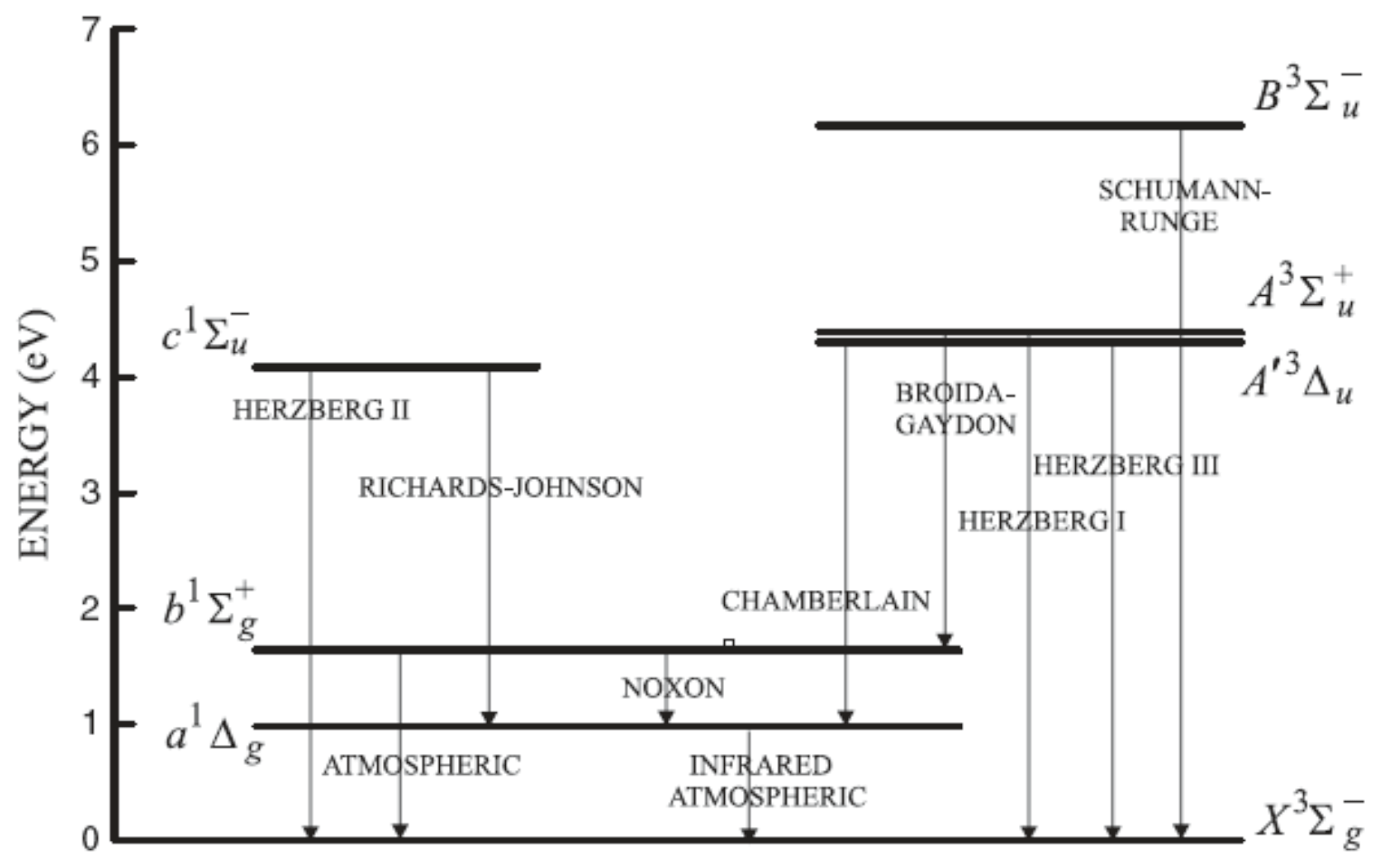
Figure A1 Energy levels of the various electronic states of the di-oxygen molecule (O₂) and names of electronic transitions between them (reprinted by permission from Springer Nature Customer Service Centre GmbH: Springer Verlag, Processes Responsible for the Occurrence of the Airglow by Vladislav Yu. Khomich, Anatoly I. Semenov, Nicolay N. Shefov, © 2008). The present study is relevant to the so-called “infrared atmospheric” transition.

A2 Observations of the 1.27 µm in the atmosphere of the Earth from the ground

One difficulty for ground-based observations of the 1.27 µm emission is that most of the emission is absorbed by O₂ before reaching the ground, letting 4 %–10 % come down to the ground. A second difficulty is that there is a strong contribution of scattered solar radiation by the atmosphere/dust. It is (now) clear what should be the optimal observing conditions:

• looking near the zenith to minimize O₂ absorption in the lower atmosphere (from a ground-based observing station located at high altitude, the O₂ absorption will be a little bit reduced) and

• looking just after the sunset, when the Sun is still illuminating the ozone layer producing this emission, between 30 and 80–90 km, but not illuminating the lower atmosphere, to avoid Rayleigh/Mie scattering which produces a strong sky background signal.

The first observation from the ground was reported by Lowe et al. (1969), followed by Baker et al. (1975) and Pendleton et al. (1996), all fulfilling the above-mentioned optimal conditions.

A3 Observations on Venus and Mars

The emission of Venus at 1.27 µm was discovered by Pierre Connes (Connes et al., 1979), then studied in particular by Crisp et al. (1996). It is due to the recombination in Reaction (3) ($\mathrm{O}+\mathrm{O}+\mathrm{M}$). On Mars, both types of emissions (2 and 3) exist. The martian ozone emission was discovered by Pierre Connes (Noxon et al., 1976), and the martian recombination emission (Reaction 3) by the OMEGA experiment aboard Mars Express (Bertaux et al., 2012).

A4 Computation of a synthetic spectrum of O₂^* emission from HITRAN 2016

The aim of this section is to describe a way to compute what could be the emission spectrum of the emission of O₂^* in the dayglow, relevant to nadir GHG daylight observations. In an early phase of the present studies in 2016, we made the following crude approximation. We computed, from HITRAN 2016 (Gordon et al., 2017), the local high-resolution spectrum of absorption by O₂ molecule at a variety of altitudes. Then, we assumed that the emission spectrum shape (but not magnitude) was identical to the absorption spectrum. In the following, we detail how we can compute more accurately a theoretical spectrum of the local emission of the O₂^* molecule from the data that are present in HITRAN 2016 line-by-line information and some additional considerations.

A4.1 Computation of the total emission rate of O₂^* molecule coming from ozone dissociation

As described in Sect. 4.1.1, the REPROBUS CTM model is used to compute the 3-D distribution of ozone as a function of space and time, based on a set of chemical reactions, solar photolysis of various species, and the actual meteorological fields of winds, temperature, and pressure procured by ECMWF.

Then, an additional model computes the photo-dissociation of ozone with the UV solar spectrum of the day, yielding to a 3-D distribution of the concentration [O₂^*] of species O₂^* (electronic state a¹Δ_g) in units of cm⁻³. As said above, the lifetime of this electronic state is about 75 min, corresponding to a spontaneous emission rate A_global of $\mathrm{1}/(\mathrm{75}\times \mathrm{60})=\mathrm{2.22}\times {\mathrm{10}}^{-\mathrm{4}}$ s⁻¹. For low altitudes, one must take into account the quenching of this excited state by collisions with all other gases (including O₂), mainly at the lowest altitudes (<50 km). Ignoring the quenching, the rate of emitted photons, VER in units of photons (cm³ s)⁻¹, may be computed from

$$\begin{array}{}\text{(A2)}& \text{VER}=A_{\mathrm{global}}\left[{{\mathrm{O}}_{\mathrm{2}}}^{*}\right].\end{array}$$

A4.2 Computation of the airglow detailed line-by-line intensity

The same principle may be applied to the detailed emission spectrum by computing a VER for each transition line L_i of the 1.27 µm band, line by line. This can be done from the data contained in the HITRAN database for this O₂ electronic transition. All the existing lines (within a certain wavelength interval) in absorption also exist in emission, and only those exist. In Eq. (A2), A_global must be replaced by the Einstein coefficient of spontaneous emission A(L_i) which is present in the HITRAN table for each transition (HITRANonline website; https://hitran.org, last access: 11 June 2020). In the present study, we have used only the ¹⁶O¹⁶O main isotope of O₂. For higher degrees of refinement that may be necessary in view of the high accuracy required on $X_{{\mathrm{CO}}_{\mathrm{2}}}$, other O₂ isotopes should also be considered.

The concentration [O₂^*(E_i)] of the O₂^* molecule must be computed in all possible energy levels E_i. E_i depends on the rotational number J^′ (J^′ for upper state, J^′′ for lower state which here is irrelevant) and the vibration number (mainly $V^{\prime }=\mathrm{0}$ but some with $V^{\prime }=\mathrm{1}$). The concentration [O₂^*(E_i)] will depend on the rotational statistical weight $\mathrm{2}{J}^{\prime }+\mathrm{1}$ and the temperature T, and is also proportional to [O₂^*].

$$\begin{array}{}\text{(A3)}& \mathrm{VER}\left(L_i\right)=A\left(L_i\right)\left[{{\mathrm{O}}_{\mathrm{2}}}^{*}(E_{i)}\right]\end{array}$$

A4.3 Computing the distribution of O₂^* molecules among the various energy levels

In their 2006 paper, Simeckova et al. (2006) describe “the calculation of the statistical weights and the Einstein A coefficients for the 39 molecules and their associated isotopologues/isotopomers currently present in the line-by-line portion of the HITRAN database”. This is all that is needed to calculate second members of Eq. (A3) for all allowed transitions L_i, giving the rate of emission of the corresponding spectral line VER(L_i).

In an approximation of a two-level system (upper m and lower n levels are denoted as 2 and 1, respectively) at LTE (local thermodynamic equilibrium), we have the well-known equations linking the Einstein A coefficients and B coefficients:

$$\begin{array}{}\text{(A4)}& {\displaystyle }{g}_{\mathrm{1}}{B}_{\mathrm{12}}=g_{\mathrm{2}}{B}_{\mathrm{21}}\text{(A5)}& {\displaystyle }{A}_{\mathrm{21}}=\mathrm{8}\mathit{\pi }h{\mathit{\nu }}^{\mathrm{3}}{B}_{\mathrm{21}},\end{array}$$

where A₂₁ (spontaneous emission) is in s⁻¹, B₁₂ (absorption) and B₂₁ (stimulated emission) are in cm³ (J s²)⁻¹, and g₁ and g₂ are the statistical weights of the levels 1 and 2, respectively.

We start from Eq. (17) of Simeckova et al. (2006) with molecules in the lower level (level 1) and the upper level (level 2) (much less numerous at atmospheric temperatures), to describe their relative distribution according to their energy level E_1i or E_2i and temperature T, the index i indicating a particular rovibrational level defined by J^′ and V^′. If N is the total number of molecules per unit volume at the temperature T, the population N_2i of one of the energy levels E_2i of the upper level (level 2) is equal to

$$\begin{array}{}\text{(A6)}& N_{\mathrm{2}i}={\displaystyle \frac{g_{\mathrm{2}i}N}{Q_{\text{tot}}\left(T\right)}}{e}^{\frac{-{\mathrm{c}}_{\mathrm{2}}{E}_{\mathrm{2}i}}{T}},\end{array}$$

and a similar equation for N_1i and the energies E_1i of the lower level (Eq. 17 of Simeckova et al., 2006). Here, Q_tot(T) is the total internal partition sum of the absorbing gas at the temperature T, $g_{\mathrm{2}i}=\mathrm{2}{J}^{\prime }+\mathrm{1}$, and E_2i is the energy of the upper state in units of wavenumber (cm⁻¹). c₂ is the second radiation constant, ${\mathrm{c}}_{\mathrm{2}}=\mathrm{h}c/{\mathrm{k}}_{\mathrm{B}}$, where c is the speed of light, h is the Planck constant, and ${\mathrm{k}}_{\mathrm{B}}=\mathrm{1.38065}\times {\mathrm{10}}^{-\mathrm{23}}$ J K⁻¹ is the Boltzmann constant.

The total number of molecules per unit volume $N=\mathrm{\Sigma }{N}_{\mathrm{1}i}+\mathrm{\Sigma }{N}_{\mathrm{2}i}$, and Q_tot(T) is the sum of $Q_{\text{tot}}^{\text{lo}}\left(T\right)$ and $Q_{\text{tot}}^{\text{up}}\left(T\right)$, respectively, the internal partition sum of the lower level and the upper level. The index i refers to all possible values of J^′, starting at $J^{\prime }=\mathrm{2}$ ($J^{\prime }=\mathrm{0}$ and $J^{\prime }=\mathrm{1}$ do not exist). We have, by definition,

$$\begin{array}{}\text{(A7)}& Q_{\text{tot}}^{\mathrm{up}}\left(T\right)={\sum }_i{g}_{\mathrm{2}i}{e}^{\frac{-{\mathrm{c}}_{\mathrm{2}}{E}_{\mathrm{2}i}}{T}}.\end{array}$$

We may find the value of Q_tot(T) in Table 1 of the paper of Simeckova et al. (2006). For instance, Q_tot(T=296 K) =215.77 for the main oxygen isotopologue ¹⁶O¹⁶O. The temperature 296 K is a reference temperature for the HITRAN database. For our purpose, we have to find $Q_{\text{tot}}^{\text{up}}\left(T\right)$ for the upper level of the transition, from a summation described in Eq. (A7). The summation must be not over all the transitions but over all energy levels. Since the HITRAN database consists in a list of transitions, some caution must be used when using the HITRAN database, in order to extract a list of energy levels. Once we have Q_tot(T), the total internal partition sum, we may then compute all values of N_2i, for the required temperature, from the distribution of the excited molecules between the various energy levels from Eq. (A6).

However, $Q_{\text{tot}}^{\mathrm{up}}\left(T\right)$ is very small when referred to all molecules N. For convenience, we have replaced in Eq. (A9) the values E_2i by E_2i−E₂₀, where E₂₀ is the energy of the lowest energy populated level with $J^{\prime }=\mathrm{2}$. With this approach, we found new values $Q{{}^{\prime }}_{\text{tot}}^{\mathrm{up}}=Q_{\mathrm{tot}}^{\mathrm{up}}\exp ({\mathrm{c}}_{\mathrm{2}}{E}_{\mathrm{20}}/T)$ for the upper level: $Q{{}^{\prime }}_{\text{tot}}^{\mathrm{up}}$(T=296 K) =147.196 for 296 K, and $Q{{}^{\prime }}_{\text{tot}}^{\mathrm{up}}$(T=200 K) =100.143. In Fig. A2, both the exponential term and the relative population are represented as a function of J^′, a product of the exponential term and the statistical weight $\mathrm{2}{J}^{\prime }+\mathrm{1}$. Only the $V^{\prime }=\mathrm{0}$ levels are kept here, because levels $V^{\prime }=\mathrm{1}$ levels are weakly populated, though they are present in the line list that are extracted from HITRAN line-by-line database in our selected wavelength interval of interest (transition (1, 1).

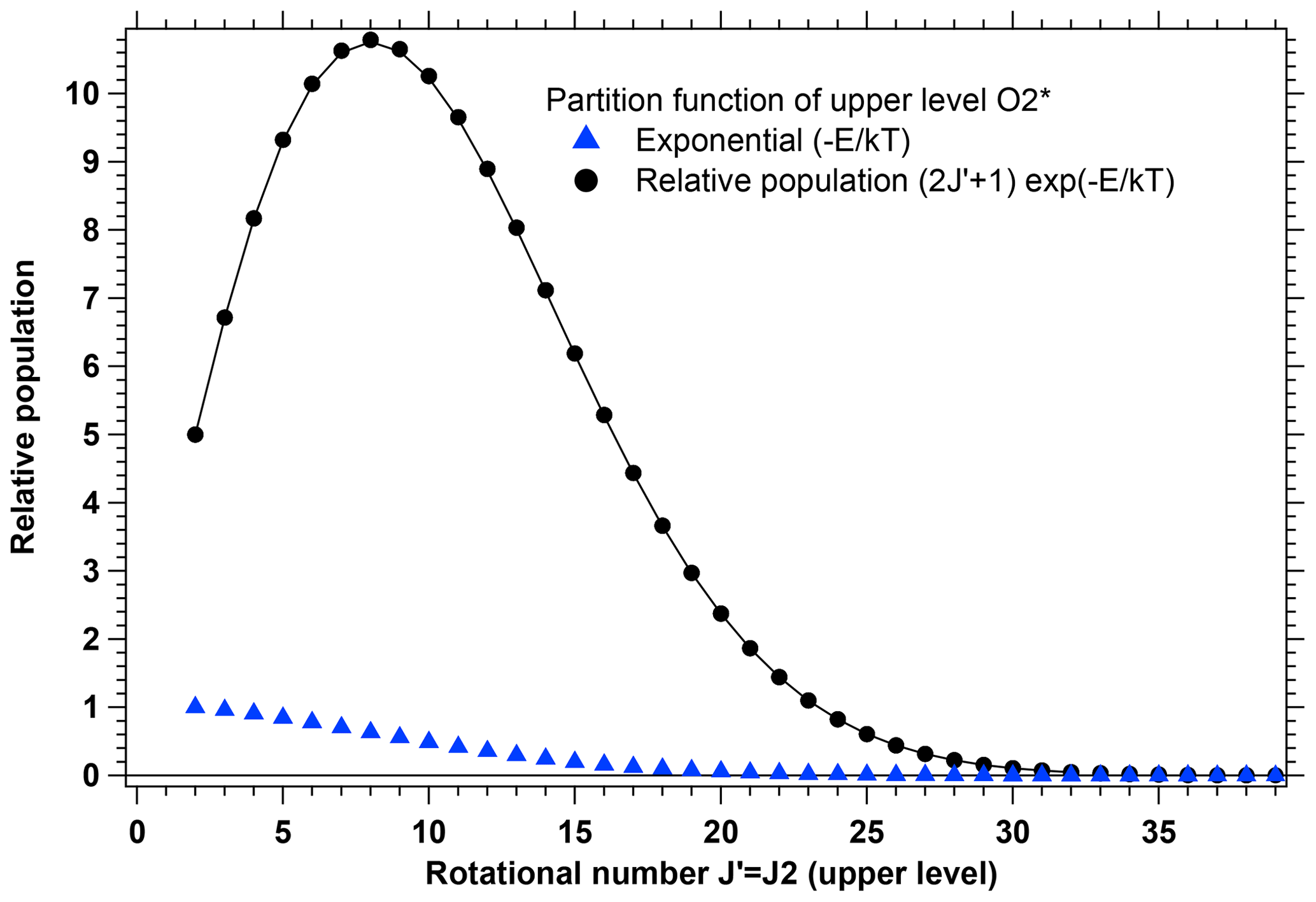
Figure A2 Partition function of the O₂^* molecule as a function of rotation state J^′ for T=296 K. Blue triangles indicate exponential terms for population, with 1 being the lowest. Black circles indicate the relative population computed from information contained in the HITRAN database of transitions. It allows to retrieve the allowed values of J^′. The first point is for $J^{\prime }=\mathrm{2}$ with a value of $\mathrm{5}=\mathrm{2}{J}^{\prime }+\mathrm{1}$, and exp (0)=1. The sum of all relative populations is $Q{{}^{\prime }}_{\text{tot}}^{\text{up}}$ by definition.

Figure A3 presents the various energy levels (in cm⁻¹) of the upper state, the O₂^* molecule. The energy is here counted above the lowest energy level of the fundamental state $X^{\mathrm{3}}{\mathrm{\Sigma }}_g^{-}$.

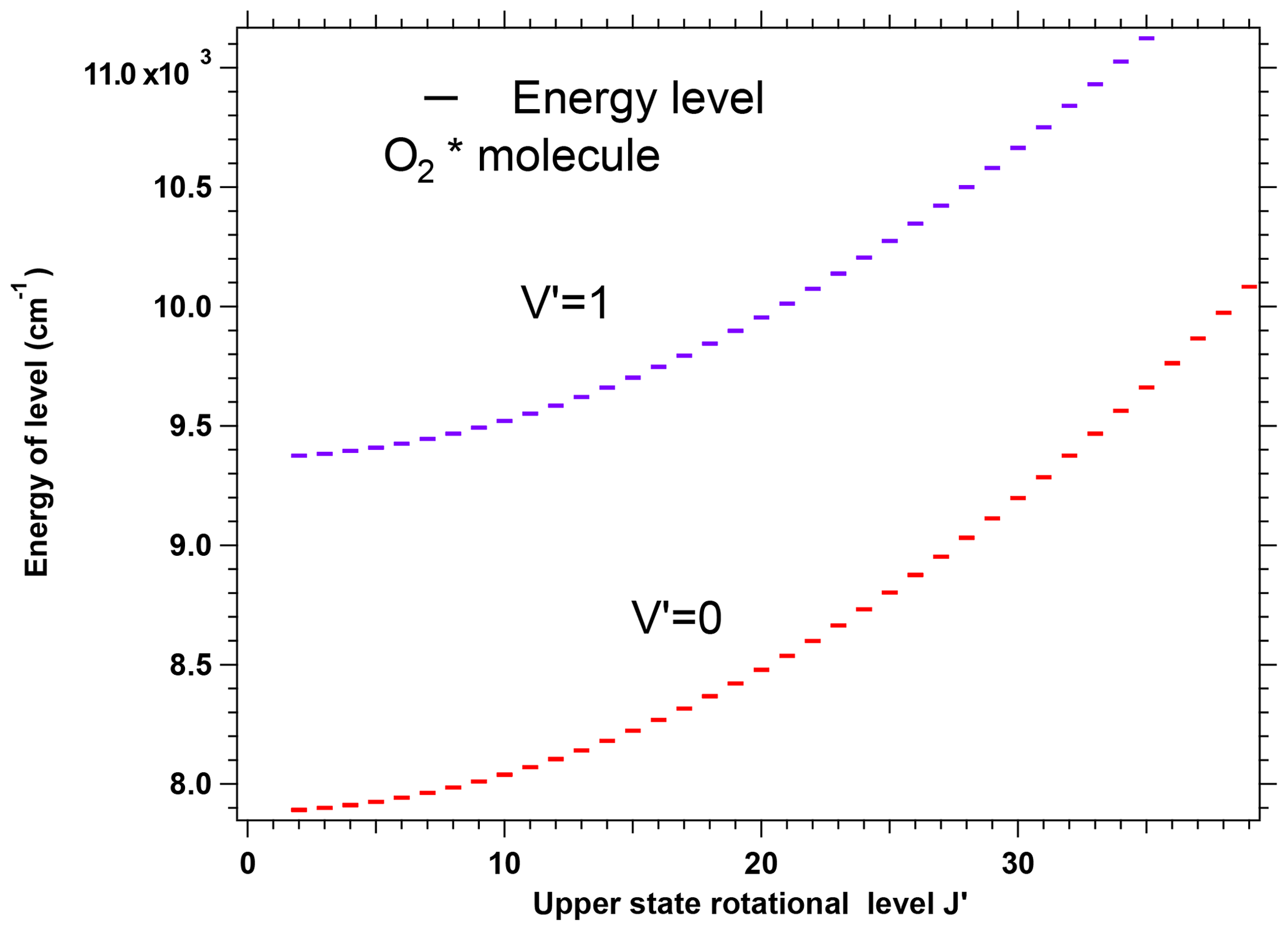
Figure A3 Energy levels (in cm⁻¹) of the excited molecule O₂* as a function of rotational and vibrational quantum numbers J^′ and V^′.

At LTE and atmospheric temperatures, $Q_{\text{tot}}^{\text{up}}\ll Q_{\text{tot}}^{\text{lo}}\approx Q_{\text{tot}}\left(T\right)$ with a factor $\frac{Q_{\text{tot}}^{\mathrm{up}}\left(T\right)}{Q_{\text{tot}}\left(T\right)}$ near 10⁻¹⁶, while $\frac{Q{{}^{\prime }}_{\text{tot}}^{\mathrm{up}}\left(T\right)}{Q_{\text{tot}}\left(T\right)}$ is approximately between 0.1 and 1.

The partition functions described above, as well as the connection between the A₂₁ and the strength of the transition S_HIT, were established with consideration of a gas at LTE conditions. But then the value of A₂₁ does not depend if there is LTE or not. In particular, when a population of excited O₂^* molecules is produced from ozone photolysis, the ratio ΣN_2i∕N may be much larger than with LTE conditions. Whatever rotational level in which they will be produced by photolysis, they will soon re-equilibrate among the various rotational upper levels because the radiative lifetime is quite long versus the collision time with ambient molecules which tend to relax to the collisional equilibrium of the various rovibrational levels, without changing ΣN_2i∕N (in the absence of quenching).

A4.4 Computing the total decay rate of the excited molecule O₂^*

The actual distribution $Q(J^{\prime },T)/Q_{\text{tot}}^{up}\left(T\right)$ of the excited molecule O₂^* is a function of the rotational state J^′ and of the temperature, such that the sum over all J^′ is equal to 1:

$$\begin{array}{}\text{(A8)}& {\displaystyle \frac{\sum Q\left(J{}^{\prime },T\right)}{Q_{\text{tot}}^{\text{up}}\left(T\right)}}=\mathrm{1}.\end{array}$$

Each particular rotational level may decay through several transitions, each transition with its own decay rate, or Einstein probability of spontaneous emission, called A₂₁, which is given in HITRAN tables of line-by-line lists. The total (average) decay rate from the upper level is obtained by summing all A₂₁ on all transitions weighted by the relative population of each rotational level:

$$\begin{array}{}\text{(A9)}& A_{\text{21\hspace{0.17em}tot}}=\sum A_{\mathrm{21}}\left(J{}^{\prime }\right){\displaystyle \frac{Q\left(J{}^{\prime },T\right)}{Q_{\text{tot}}^{\mathrm{up}}\left(T\right)}}.\end{array}$$

Since there is the emission of one photon around 1.27 µm for each decay of one excited O₂^* molecule, A_21 tot is the weighted sum of all rates of all transitions going down, which is the total emission rate, the total number of photons emitted in the whole band per second by a single molecule of O₂^*.

Then, we must multiply by the number density of O₂^* to get the volume emission rate in photons (cm³ s)⁻¹. We found from the HITRAN data that the total decay rate is $A_{\text{21\hspace{0.17em}tot}}=\mathrm{2.29}\times {\mathrm{10}}^{-\mathrm{4}}$ s⁻¹, slightly different from $\mathrm{2.22}\times {\mathrm{10}}^{-\mathrm{4}}$ s⁻¹ derived from the rounded value of 75 min of the lifetime quoted by Lafferty et al. (1998). We may compute the lifetime $\mathrm{1}/A_{\text{21\hspace{0.17em}tot}}=\mathrm{4367}$ s ∼73 min. The excited molecule O₂^* will, in average, stay excited for more than 1 h (in the absence of quenching, de-excitation by collisions without the emission of one photon; not addressed here).

It must be realized that it is experimentally very difficult to measure directly such a long lifetime. Instead, because the values of A₂₁ are connected to the values of absorption coefficients B₂₁, it is easier to measure the absorption of O₂ molecules and then make the appropriate calculations to derive the A₂₁ values, according to principles explained in Simeckova et al. (2006), which have been used to fill the HITRAN line-by-line lists with A₂₁ rates for each transition.

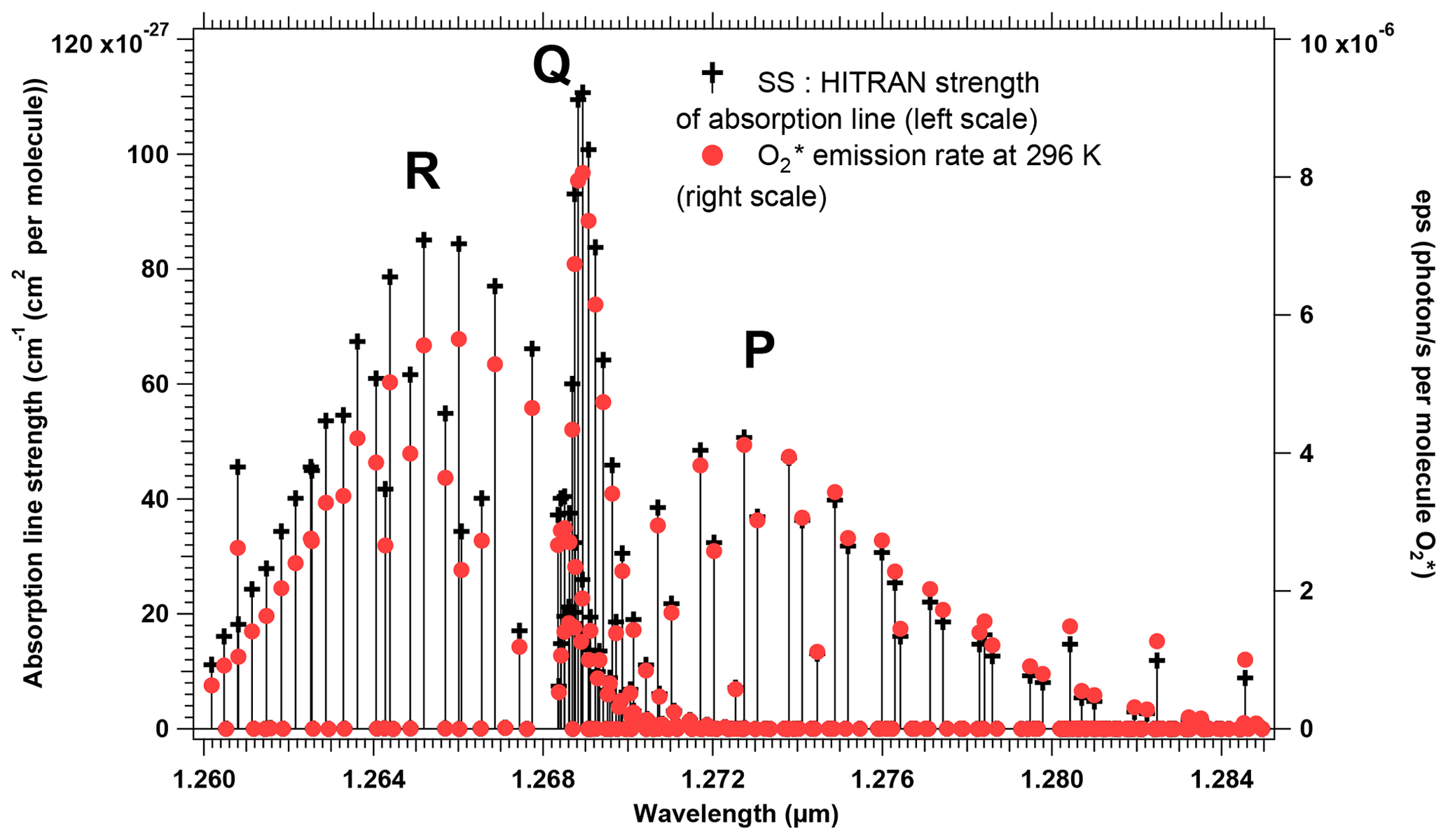
Figure A4 Emission rate per excited molecule O₂${}^{*}\mathrm{eps}=\mathit{\epsilon }\left(k\right)$ from Eq. (13) in photons s⁻¹ per molecule O₂^* (left scale) compared to the absorption line strength SS at 296 K found in HITRAN data (in units of cm⁻¹ (cm² per molecule)). See text for more explanations.

A4.5 Computing the emission spectrum of the excited molecule O₂^*

The emission rate per O₂^* molecule ε(k) of a transition k is obtained by multiplying the Einstein coefficient A₂₁(k) by the relative population of the upper level:

$$\begin{array}{}\text{(A10)}& \mathit{\epsilon }\left(k\right)=A_{\mathrm{21}}\left(k\right){\displaystyle \frac{Q\left(J{}^{\prime }\left(k\right),T\right)}{Q_{\text{tot}}^{\text{up}}\left(T\right)}}.\end{array}$$

When plotted as a function of wavelength of transition k, it represents the emission spectrum for one molecule, per molecule and per second. It is displayed in Fig. A4 for 296 K (right scale) and compared to the absorption line intensities SS which are found in the line-by-line HITRAN line list (left scale). The distribution of the lines in three branches is clearly observed (Q branch: $J^{\prime }-J^{\prime \prime }=\mathrm{0}$; P branch: $J^{\prime }-J^{\prime \prime }=-\mathrm{1}$; R branch: $J^{\prime }-J^{\prime \prime }=+\mathrm{1}$). The transitions from $V^{\prime }=\mathrm{1}$ to $V^{\prime \prime }=\mathrm{1}$ are very weak and near the zero line.

Therefore, a spectrum of the local emission in the band could be computed by describing each emission transition by a Gaussian with an appropriate width (associated with the temperature), adding all transitions to form a full spectrum, and multiplying by the actual density of O₂^* molecules.

However, we have implemented another method to take advantage of LBLRTM software (Clough and Iacono, 1995) which computes for the terrestrial atmosphere absorption spectra (either local or integrated over one LOS) from the HITRAN database. Indeed, with the adequate scaling of both the right and left scales of Fig. A4, it is noted that the strength of absorption lines are just above the emission rates on the left side of the graph (short wavelength), while it is the reverse on the right side. As we shall see below, there is a theoretical reason for this progressive change of the emission-to-absorption-strength ratio.

A4.6 Theoretical computation of the emission ∕ absorption ratio

We first repeat here Eq. (19) from Simeckova et al. (2006), which links A₂₁ to the line strength SS (below, S_ν(k, T)) in which k designates one transition from energy level E_1k with a wavenumber ν₀:

$$\begin{array}{}\text{(A11)}& \begin{array}{rl}{S}_{\mathit{\nu }}(k,T)=& {\displaystyle \frac{g_{\mathrm{2}}}{Q_{\text{tot}}\left(T\right)}}{\displaystyle \frac{A_{\mathrm{21}}\left(k\right)}{\mathrm{8}\mathit{\pi }c{\mathit{\nu }}_{\mathrm{0}}^{\mathrm{2}}}}\exp \left({\displaystyle \frac{-{\mathrm{c}}_{\mathrm{2}}{E}_{\mathrm{1}k}}{T}}\right)\\ & \left(\mathrm{1}-\exp \left({\displaystyle \frac{-{\mathrm{c}}_{\mathrm{2}}{\mathit{\nu }}_{\mathrm{0}}}{T}}\right)\right).\end{array}\end{array}$$

We may extract the expression of A₂₁(k) from Eq. (A11) and put it in Eq. (A10). Taking into account that $E_{\mathrm{2}k}-E_{\mathrm{1}k}={\mathit{\nu }}_{\mathrm{0}}$ and that the relative population of energy level E_2k is

$$\begin{array}{}\text{(A12)}& \begin{array}{rl}Q\left(J{}^{\prime }\left(k\right),T\right)& =\left(\mathrm{2}J{}^{\prime }+\mathrm{1}\right)\exp \left(-{\displaystyle \frac{{\mathrm{c}}_{\mathrm{2}}{E}_{\mathrm{2}k}}{T}}\right)\\ & =g_{\mathrm{2}}\exp \left(-{\displaystyle \frac{{\mathrm{c}}_{\mathrm{2}}{E}_{\mathrm{2}k}}{T}}\right),\end{array}\end{array}$$

we could find a very simple result on the ratio of emission ε(k) to absorption line strength S_ν(k, T) for each line:

$$\begin{array}{}\text{(A13)}& {\displaystyle \frac{\mathit{\epsilon }\left(k\right)}{S_{\mathit{\nu }}(k,T)}}=\mathrm{8}\mathit{\pi }c{\mathit{\nu }}_{\mathrm{0}}^{\mathrm{2}}{\displaystyle \frac{Q_{\text{tot}}\left(T\right)}{Q_{\text{tot}}^{\mathrm{up}}\left(T\right)}}{\displaystyle \frac{\mathrm{1}}{\exp \left(\frac{{\mathrm{c}}_{\mathrm{2}}{\mathit{\nu }}_{\mathrm{0}}}{T}\right)-\mathrm{1}}}.\end{array}$$

In Fig. A5, the ratio of our calculated emission to the HITRAN line strength SS for all transitions within our spectral interval is plotted for two temperatures (black and blue dots), together with the analytical formula (Eq. A13) (a continuous function of wavenumber ν₀) computed on a regular wavelength grid. Both share the same scale on the left: there is a perfect coincidence, which validates our derivation of Eq. (A13).

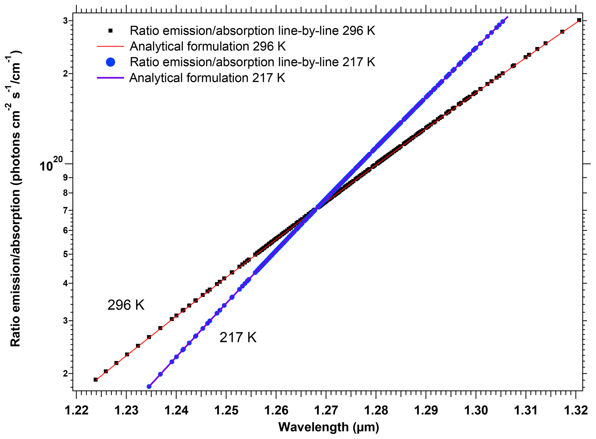
Figure A5 For two different temperatures (296 and 217 K), the ratios of our calculated emission rate to the HITRAN line strength SS are plotted (respectively, black and blue dots) for all 375 transitions of HITRAN table (between 1.2238 and 1.32068 µm). The solid lines (respectively, red and blue) are computed from the analytical formula (Eq. A13) on a grid of wavelength–wavenumber using the same scale on the left as the ratio of emission to line strength in units of photons cm⁻² s⁻¹ ∕ cm⁻¹, where cm⁻¹ is a wavenumber unit.

A4.7 Practical method to produce a synthetic emission spectrum

In order to simulate a local emission spectrum, we could use the method exposed above in Appendix A4.5, giving the emissivity per molecule O₂^* for each line, and then distribute this emissivity over a Gaussian attached to each line and add all line contributions spectrally. We have developed another method, capitalizing on the capabilities of LBLRTM software (Clough and Iacono 1995). With LBLRTM, we may compute a local absorption spectrum of O₂ (for instance, computing the vertical atmospheric transmission between 67 and 68 km altitude, Tr(λ)). This transmission is linked to the local absorption a(λ) by

$$\begin{array}{}\text{(A14)}& {\displaystyle }\mathrm{Tr}\left(\mathit{\lambda }\right)=\exp \left(-a\left(\mathit{\lambda }\right)\mathrm{d}z\right)\text{(A15)}& {\displaystyle }\begin{array}{rl}& \text{or}\\ & a\left(\mathit{\lambda }\right)=-{\displaystyle \frac{\ln \left(\text{Tr}\left(\mathit{\lambda }\right)\right)}{\mathrm{d}z}}.\end{array}\end{array}$$

The shape of the local emission spectrum E_m(λ) of O₂^* molecules is then obtained by multiplying a(λ) by Eq. (A13) of the ratio of emission to absorption (ε∕ SS), which depends only of the wavenumber ν and temperature T, according to a continuous function. The wavenumber ν in cm⁻¹ is equal to 10 000 ∕ λ (in µm). Then, the obtained local emission spectrum E_m(λ) has to be normalized (by integration over wavelength) to the actual VER for which we wish to compute the local emission rate spectrum, yielding E_mn(λ) where the letter n stands for “normalized”.

The advantage of this approach is that LBLRTM computes the local absorption spectrum with a number of effects (line broadening, pressure shifts, Gaussian profiles, etc.) that may become non-negligible at low altitudes. Applying Eq. (A13) on the continuous spectrum, instead of applying it to the discrete set of wavelengths of each transition is justified by the fact that ν and Eq. (A13) vary very little over the spectral extent of one individual line.

In order to compute the brightness spectrum of the O₂^* emission along any LOS, one has to integrate E_mn(λ) over length through the atmosphere. The “self-absorption” by O₂ molecules along the LOS must be accounted for, except in regions where it is negligible (high altitudes, say >80 km).

Appendix B: Retrieval of O₂(¹Δ) VER from SCIAMACHY limb radiances

We have developed a numerical scheme to retrieve the vertical distribution of the O₂(¹Δ) VER from a series of limb radiances obtained during a SCIAMACHY limb scan, taking into account the absorption along the LOS by background O₂ of the O₂(¹Δ) emission between the location of the emission and the spacecraft (sometimes this O₂ absorption is called self-absorption, improperly in our opinion, because the O₂(¹Δ) molecule is different from the background O₂, as long as it is in the excited state (¹Δ)).

B1 The case with no absorption: the onion-peeling technique

When there is no absorption, the radiance B is related to the integral along the LOS of the VER (or emissivity) ε(s), s being an abscissa along the LOS.

$$\begin{array}{}\text{(B1)}& B={\displaystyle \frac{\mathrm{1}}{\mathrm{4}\mathit{\pi }}}\int \mathit{\epsilon }\left(s\right)\mathrm{d}s\end{array}$$

B is the wavelength-integrated spectral radiance, expressed in photons (cm² s sr)⁻¹, while ε(s) is here spectrally integrated and expressed in photons (cm³ s)⁻¹.

A classical way to retrieve a vertical distribution of ε from a series of radiance measurements at the limb is the onion-peeling method (Fig. B1), which assumes that the emissivity (or VER) is locally spherically symmetric, depending only on the altitude. Furthermore, the problem is discretized by dividing the atmosphere in spherical layers, in which the VER is constant.

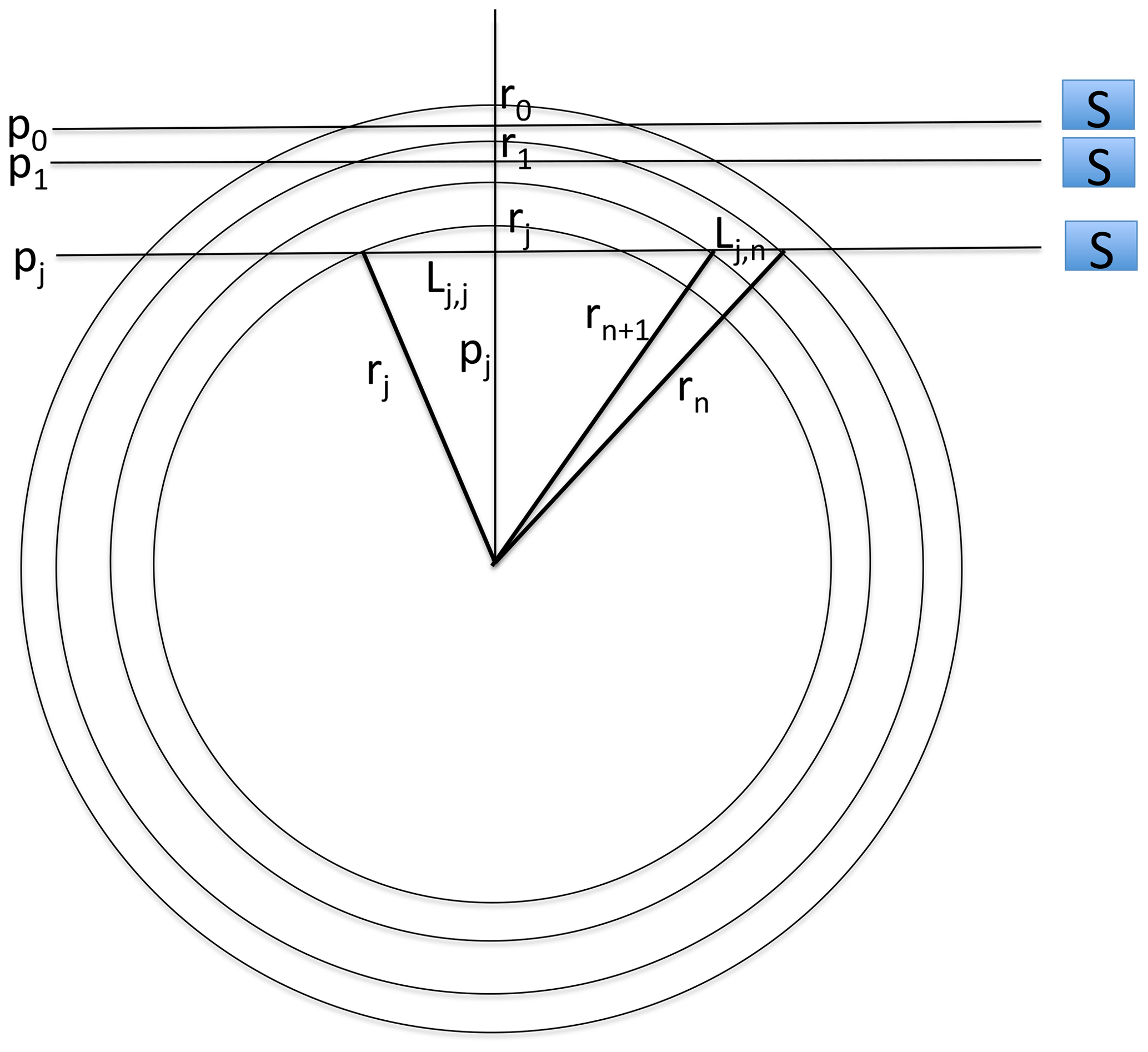
Figure B1 Geometry of the LOS at the limb of an emission organized in spherical layers. The various LOS are obtained either by drifting the observer S into an orbit with a fixed inertial direction (case of GOMOS/Envisat) or by angular scanning (case of SCIAMACHY/Envisat).

Let p₀, … p_j be the series of impact parameters of viewing LOS with p= tangent altitude z+R_earth, p₀ the largest. We define a series of spheres with r₀>p₀ and decreasing radii. Let $L_{j,n}=$ length of one of the two equal segments (j, n) between spheres of radius r_n and r_n+1 along the LOS with impact parameter p_j.

We have the following expressions (B2):

$$\begin{array}{}\text{(B2)}& \begin{array}{rl}& L_{\mathrm{0},\mathrm{0}}=\sqrt{r_{\mathrm{0}}^{\mathrm{2}}-p_{\mathrm{0}}^{\mathrm{2}}}\\ & L_{\mathrm{1},\mathrm{1}}=\sqrt{r_{\mathrm{1}}^{\mathrm{2}}-p_{\mathrm{1}}^{\mathrm{2}}}\\ & L_{\mathrm{1},\mathrm{0}}=\sqrt{r_{\mathrm{0}}^{\mathrm{2}}-p_{\mathrm{1}}^{\mathrm{2}}}-L_{\mathrm{1},\mathrm{1}}\\ & \mathrm{\dots }\\ & L_{j,n}=\sqrt{r_n^{\mathrm{2}}-p_j^{\mathrm{2}}}-\sqrt{r_{n+\mathrm{1}}^{\mathrm{2}}-p_j^{\mathrm{2}}}.\end{array}\end{array}$$

For the last segments when j=n, the formula is slightly different because the sphere of radius r_j+1 is irrelevant:

$$L_{j,j}=\sqrt{r_j^{\mathrm{2}}-p_j^{\mathrm{2}}}.$$

The radiances B(p) may then be expressed (B3) as a function of ε(z):

$$\begin{array}{}\text{(B3)}& \begin{array}{rl}& B\left(p_{\mathrm{0}}\right)={\displaystyle \frac{\mathrm{1}}{\mathrm{4}\mathit{\pi }}}\mathit{\epsilon }\left(z_{\mathrm{0}}\right)\cdot \mathrm{2}\cdot L_{\mathrm{0},\mathrm{0}}\\ & B\left(p_{\mathrm{1}}\right)={\displaystyle \frac{\mathrm{1}}{\mathrm{4}\mathit{\pi }}}\left[\mathit{\epsilon }\left(z_{\mathrm{0}}\right)\cdot \mathrm{2}\cdot L_{\mathrm{1},\mathrm{0}}+\mathit{\epsilon }\left(z_{\mathrm{1}}\right)\cdot \mathrm{2}\cdot L_{\mathrm{1},\mathrm{1}}\right]\\ & \mathrm{\dots }\\ & B\left(p_n\right)={\displaystyle \frac{\mathrm{1}}{\mathrm{4}\mathit{\pi }}}\left[\mathrm{2}\sum _k\mathit{\epsilon }\left(z_k\right)L_{n,k}\right].\end{array}\end{array}$$

This is a linear system of n equations with the n unknowns ε(z_j). This system may be written under a matrix form 4πB=M ε, M being a triangular matrix of order n, the number of atmospheric layers. Elements of the matrix are the lengths of LOS segments within a layer between two spherical shells. Therefore, the matrix may be simply inverted to yield the vector ε from the vector of measurements B:

$$\begin{array}{}\text{(B4)}& \mathit{\epsilon }=\mathrm{4}\mathit{\pi }{\mathbf{M}}^{-\mathrm{1}}\mathbf{B}.\end{array}$$

B2 The case with absorption: a modified onion-peeling technique

When absorption by O₂ is considered, Eq. (18) is modified into

$$\begin{array}{}\text{(B5)}& B={\displaystyle \frac{\mathrm{1}}{\mathrm{4}\mathit{\pi }}}\int \mathit{\epsilon }\left(s\right)\exp (-\mathit{\tau }(s\left)\right)\mathrm{d}s,\end{array}$$

where τ(s) is the optical thickness between the emission point and the observer (here assumed to be outside of the atmosphere). The corresponding attenuation factor is

$$\begin{array}{}\text{(B6)}& \mathrm{Tr}\left(s\right)=\exp \left(-\mathit{\tau }\left(s\right)\right).\end{array}$$

In reality, ε, τ(s), Tr(s), and B all depend on wavelength λ. However, the quantities τ(s, λ), Tr(s, λ) may be computed for a given atmospheric model defined by a vertical profile of temperature T(z) and pressure p(z), with the dry air density $n\left(z\right)=p\left(z\right)/k$ T(z) and O₂ density 0.2095 n(z). We made use of the LBLRTM code and HITRAN2016 database to conduct such computations.

The detailed spectral shape of the local emission of the O₂^* molecule ε(z, λ) may be computed from the analysis of Appendix A. Therefore, we can compute a wavelength-integrated attenuation factor between the emission location and the external observer, independent of the actual value of the local $\text{VER}\left(z\right)=\int \mathit{\epsilon }(z,\mathit{\lambda })\mathrm{d}\mathit{\lambda }$ for every cell of the onion-peeling scheme described above. We keep the matrix approach, but now each element of the matrix is a length of a segment multiplied by the pre-calculated attenuation factor. While in the standard onion-peeling scheme, there are two identical segments, symmetric with regard to the tangent point, giving equal contributions to the observed intensity; the attenuation factor is different for the two segments (one in the foreground, the other in the background).

For a given limb observation, each SCIAMACHY spectrum is integrated in wavelength to yield the total limb radiance measurements B(z), and Eq. (B4), where M matrix is modified to include the attenuation factor, is used to derive the vertical profile of the volume emission rate ε(z). It may be shown that the attenuation factor FAS_j, n affecting both foreground and background segments on one LOS may be written as

$$\begin{array}{}\text{(B7)}& \begin{array}{rl}& {\mathrm{FAS}}_{j,n}=\\ & \mathrm{0.5}{\displaystyle \frac{\int {\mathit{\tau }}_{\text{km}}\left(z_n,\mathit{\lambda }\right)\cdot \left[\exp \left(-{\mathit{\tau }}_{j,n}^{\mathrm{f}}\left(\mathit{\lambda }\right)\right)+\exp \left(-{\mathit{\tau }}_{j,n}^{\mathrm{b}}\left(\mathit{\lambda }\right)\right)\right]\mathrm{d}\mathit{\lambda }}{\int {\mathit{\tau }}_{\text{km}}(z,\mathit{\lambda })\mathrm{d}\mathit{\lambda }}},\end{array}\end{array}$$

where τ_km(z_nλ) is the optical thickness per kilometre of O₂ absorption at wavelength λ and altitude z_n, ${\mathit{\tau }}_{j,n}^{\mathrm{f}}\left(\mathit{\lambda }\right)$ and ${\mathit{\tau }}_{j,n}^{\mathrm{b}}\left(\mathit{\lambda }\right)$ are, respectively, for the foreground segment and the background segment the optical thickness of O₂ absorption from the segment to the observer, along the LOS.

B3 Comparison of methods used by others

Zarboo et al. (2018) have also used the SCIAMACHY limb scans in order to retrieve the vertical profile of the O₂^* emissivity. However, their technique is quite different. They find a best fit to the whole series of observed spectra with a model of the vertical distribution of spectral emissivity, but they do not account for attenuation by O₂. Therefore, they must underestimate their emissivities more and more with lower altitudes. Their method does not need to know the state of the atmosphere nor the theoretical shape of the emissivity; in principle, if their SNR would be large enough, they could interpret the spectral shape of their retrieved emissivities in terms of local temperature, by comparing with model predictions built on our approach developed in Appendix A. Because they have used a special SCIAMACHY mode of observation dedicated to the MLT, in which the scanning at the limb is in the range of 50–150 km, the fact that they did not account for O₂ re-absorption along the LOS is probably not very important. They have limited their study to altitudes >50 km.

Sun et al. (2018) have studied also the SCIAMACHY spectra in the O₂^* band for the same purpose as us: for a better retrieval of the $X_{{\mathrm{CO}}_{\mathrm{2}}}$ mixing ratio. In order to retrieve the spectral emissivities at each altitude, they have developed two methods. The first one (they call it “linear inversion”) is identical to the method of Zarboo et al. (2018) and does not account for O₂ absorption. In their second method (they call it “onion-peeling”), they account for O₂ absorption, except for the two tangent heights where absorption is negligible, from which they can derive the local temperature T by comparison with a model of the spectral local emissivity quite similar to what we developed in Appendix A. Then, they use the Mass Spectrometer – Incoherent Scatter (MSIS) model pressure to get the O₂ density to compute the absorption in the second layer from the top and propagate downward the computations. They can therefore compute the vertical temperature profile at each altitude.

B4 Sensitivity of VER retrieval to the choice of atmospheric model and nadir radiance estimate

In our retrieval scheme of VER from observed limb radiances, an atmospheric model is needed to compute the absorption by background O₂. We tested the sensitivity of the VER retrieval to the choice of the atmospheric model, as shown in Fig. B2 for a SCIAMACHY limb observation obtained on 1 January 2007 (at latitude of −39.9^∘ and SZA of 37.2^∘, from product 20070101_1256). The various VER profiles were obtained either with US STANDARD (a mean model for all seasons and latitudes), or with the variants SUBARCTIC_SUMMER, SUBARCTIC_WINTER, and MIDLAT_SUMMER (this last one should correspond best to the conditions of this particular observation). The relative differences may reach ±10 % between 40 and 60 km, with smaller differences above 60 km (less absorption) and larger differences below 35 km (more absorption, but regardless the VER is small). Therefore, for our following studies of many SCIAMACHY limb scans, we have systematically used the most relevant standard profile, according to the latitude and season: a so-called CLIMATO_ADAPTED atmospheric profile (“adapted climatology”).

In particular, for each studied limb scan, we have first inverted the SCIAMACHY limb total radiances to retrieve a VER vertical distribution. Then, we could compute what would be the nadir radiance in the O₂ band that should have been observed with such a profile, to simulate the MicroCarb geometry of observation or any other GHG monitoring system. The vertical integration was done above 30 km up to 80 km to be consistent with REPROBUS model which stops at 80 km. Absorption by O₂ may be computed in the nadir-viewing geometry, though attenuation in this geometry (altitude z>30 km) is small (2 % for the Q branch; less outside of the Q branch).

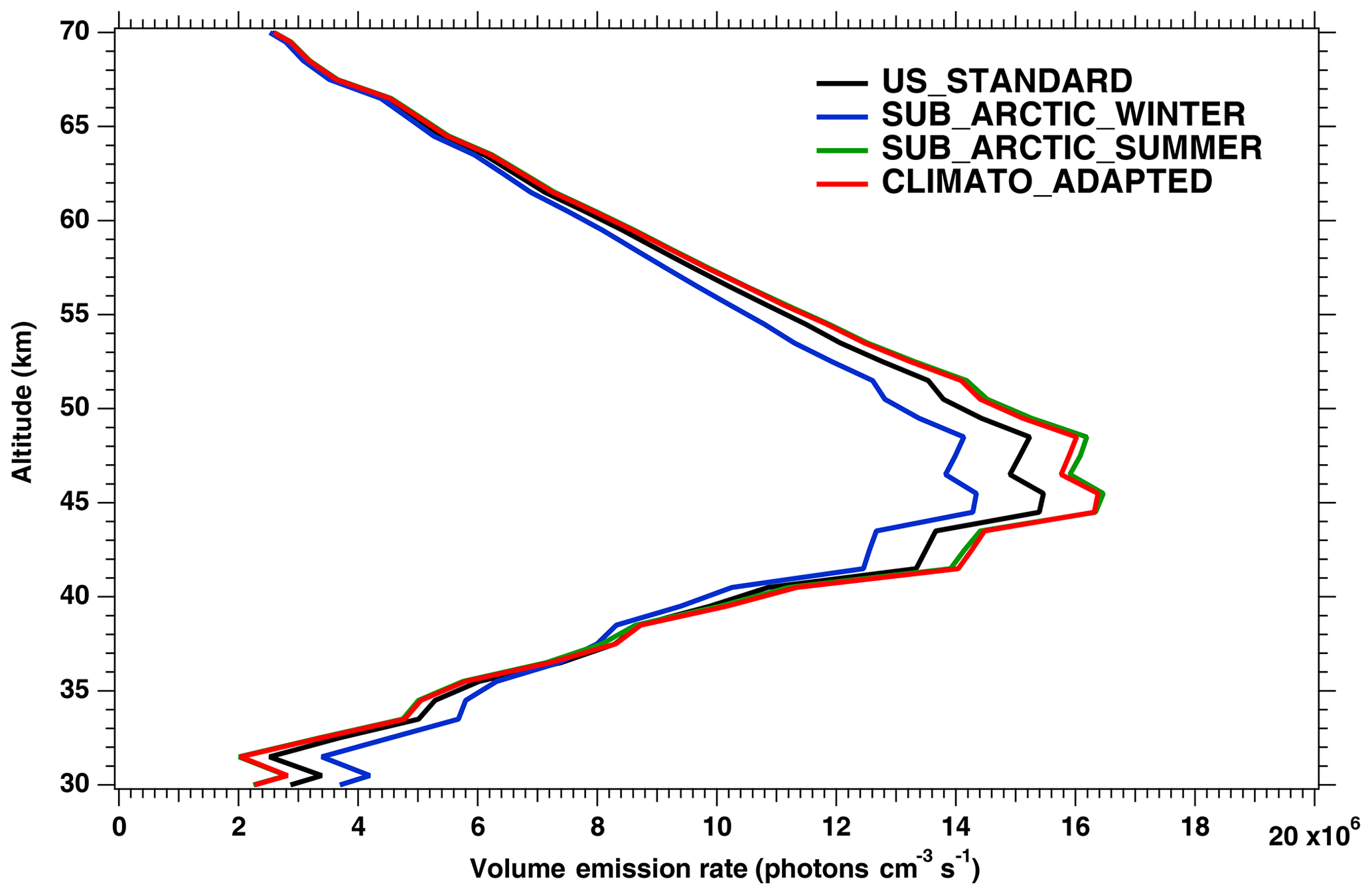
Figure B2 VER airglow profiles obtained by taking into account O₂ absorption using a climatological atmospheric profile: SUBARCTIC_SUMMER (green curve), SUBARCTIC_WINTER (blue curve), US STANDARD (black curve), and CLIMATO_ADAPTED (red curve). In the case of this profile measured in January at latitude of −39.9^∘, the adapted climatology corresponds to the MIDLAT-SUMMER climatology.

Appendix C: Comparison of measured (GOMOS) and modelled (REPROBUS) ozone vertical profiles

The photo-dissociation of ozone is the main mechanism for producing O₂(a¹Δ) airglow in the atmosphere. It is therefore important that the ozone profile calculated by the REPROBUS model is accurate. In order to verify this condition, comparisons were carried out with the ozone profiles measured by the GOMOS instrument aboard Envisat. GOMOS (Bertaux et al., 2010) measured ozone profiles by the stellar occultation method under night and day illumination conditions. For daytime occultations, there is a contaminating signal both from the illuminated limb and from the nadir emission scattered by the GOMOS baffles. Though the processing pipelines have been designed to correct for these contaminations, the resulting uncertainties in ozone density retrieval may be larger, depending on the geometrical conditions of the occultation and the altitude, lower altitudes having more stray light. Therefore, we are separating night and day conditions for the comparison.

C1 Nighttime ozone profiles

One example of REPROBUS and GOMOS individual ozone concentration profiles under night conditions for Envisat orbit no. 25402 (8 January 2007) is presented in Fig. C1. Figure C1a displays the ozone concentration measured by GOMOS and predicted by REPROBUS at the same time and location. As seen on a log scale (in order to accommodate the 5 orders of magnitude of variation of ozone with altitude), the agreement is remarkable between GOMOS and REPROBUS in the altitude range of 15–65 km. Even wiggles in the vertical profiles in the range of 15–65 km are present both in the model and in the data. Figure C1b represents the relative difference $(\text{GOMOS}-\text{REPROBUS})/\text{REPROBUS}$ on a linear scale.

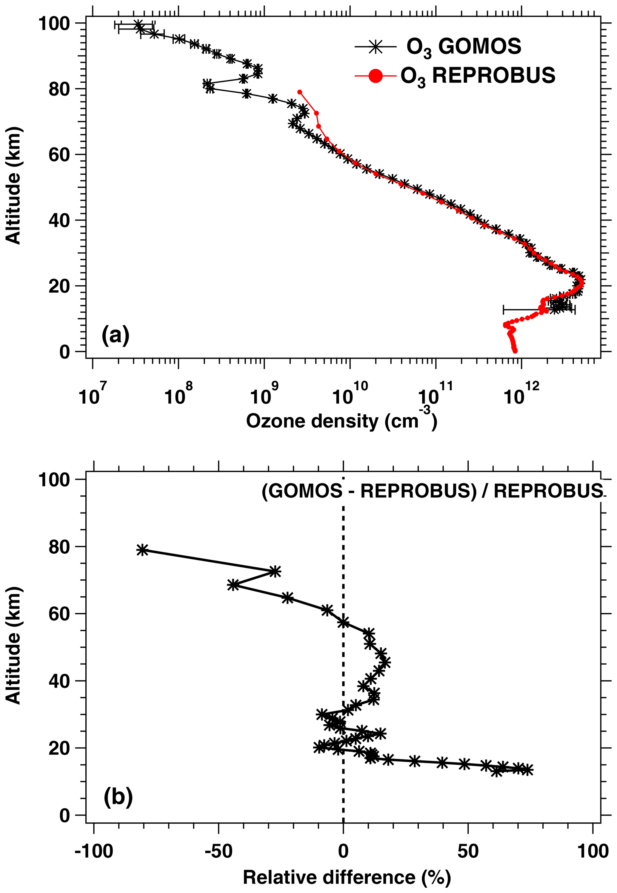
Figure C1 (a) One typical example of comparison of a GOMOS vertical ozone profile (black curve) versus REPROBUS prediction (red curve). The GOMOS profile was observed during the night on 8 January 2007. (b) Relative difference $(\text{GOMOS}-\text{REPROBUS})/\text{REPROBUS}$.

There is a significant difference above 60 km, where REPROBUS overestimates the amount of ozone relative to GOMOS. At night, GOMOS ozone profiles show a strong ozone minimum around 80 km. This is a true feature, which can be seen directly on the light of the star that increases again when the LOS passes at this altitude during the occultation of the star. This ozone “hole”, explained by loss reactions with OH radicals at night, is not reproduced by REPROBUS. The reason for this discrepancy is the assumption in the model that ozone concentration is much larger than atomic oxygen at night and thus can be set as equal to the odd oxygen family (i.e. ${\mathrm{O}}_{\mathrm{3}}\simeq {\mathrm{O}}_{\mathrm{3}}+\mathrm{O}={\mathrm{O}}_x$). This approximation is justified in the stratosphere and the lower mesosphere but is wrong in the upper mesosphere, where oxygen atoms have a lifetime of the order of a day and a concentration similar to ozone during the night (e.g. Brasseur and Solomon, 2005). This shortcoming of REPROBUS will be corrected in the next version of the model. It must be noted, however, that this O₃ overestimation in the upper mesosphere by REPROBUS only occurs in nighttime conditions.

Below 20 km, the REPROBUS and GOMOS (night) curves are also diverging. Occultation measurements are less accurate below 15–20 km, because of the attenuation of the star signal, so this difference must be considered with caution. In any case, this bias is not relevant to our study since the airglow of O₂(a¹Δ) is negligible below 30 km.

We then compared all GOMOS ozone profiles in night occultation for 2007 with REPROBUS for six different stars and plotted the relative difference $(\text{GOMOS}-\text{REPROBUS})/\text{REPROBUS}$ for the four brightest stars in Fig. C2.

The general trends observed in Fig. C2 are fairly similar for the four stars and in line with what is observed in the single profile of Fig. C1. The overestimation of ozone by the REPROBUS model above 60 km is confirmed.

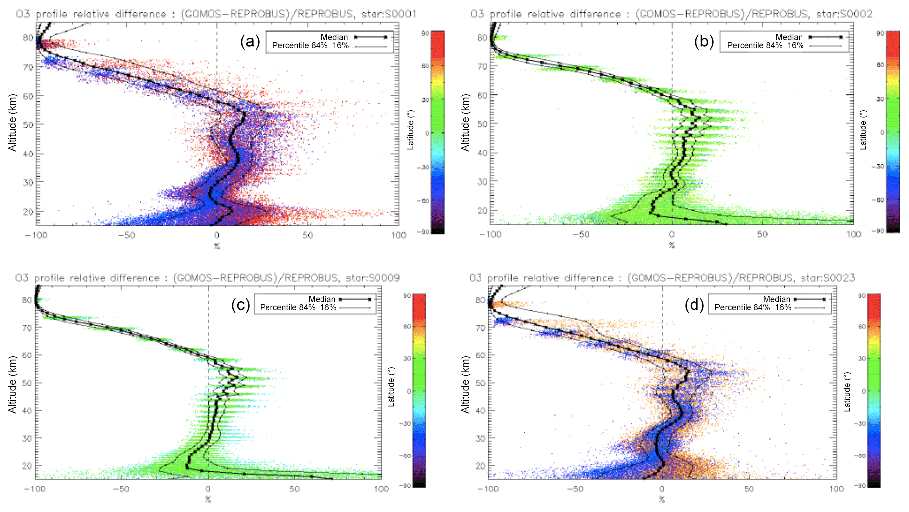
Figure C2 Relative difference between the GOMOS and REPROBUS ozone nighttime profiles for all 2007 occultations of the four brightest stars (S0001, S0002, S0009, and S0023), represented here, respectively, in panels (a), (b), (c), and (d). Each dot represents one GOMOS measurement of ozone. The colour of the dot is related to the latitude of each profile (see the colour scale). The thick black line represents the median and the thin black lines represent the 16th and 84th percentiles of the distribution of the relative difference.

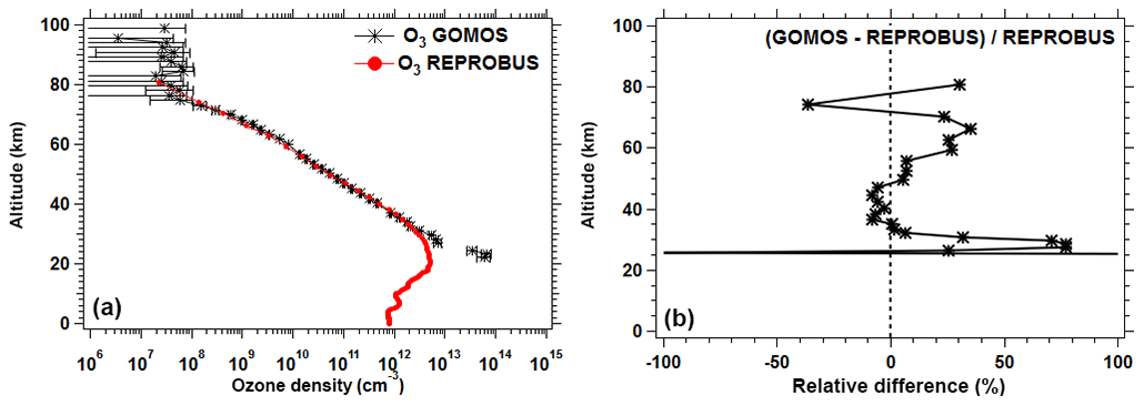
Figure C3 (a) One example of comparison of a GOMOS vertical dayside ozone profile (black curve) versus REPROBUS prediction (red curve). The GOMOS profile was observed on 5 August 2007, at an SZA of 38^∘. (b) Relative difference $(\text{GOMOS}-\text{REPROBUS})/\text{REPROBUS}$.

Below 60 km, there is an underestimation of ozone in REPROBUS relative to GOMOS with a maximum of about −15 % at 55 km, which gradually decreases to 0 % at 20 km. At the location of the maximum airglow (45–50 km), the bias is about −8 % to −10 %. This lack of ozone in REPROBUS is a major reason to explain why the airglow emission estimated by model is lower than observed by SCIAMACHY (Fig. 11). However, some exercises done by arbitrarily multiplying the REPROBUS O₃ profiles by a factor of 1.2 (not shown here) show a small remaining underestimation of the airglow calculated by the model. This discrepancy certainly warrants future detailed studies that are well beyond the scope of the present paper.

C2 Daytime ozone profiles

During the day, one comparison of REPROBUS to GOMOS observations is displayed in Fig. C3 for an SZA of 38^∘. There is a deficit (∼20 %) of ozone in REPROBUS versus GOMOS around 60 km. However, high-quality dayside data are scarce with GOMOS, and definitive conclusions cannot be drawn at this stage.

We may summarize the comparisons GOMOS/REPROBUS with the following points:

• In principle, only dayside ozone is relevant for the prediction of O₂^* airglow at 1.27 µm.

• GOMOS ozone concentration vertical profiles show quite similar values below 60 km between day and night, and larger values of O₃ at night above 60 km, a feature well understood from mesospheric chemistry.

• There is a known shortcoming of the chemistry of REPROBUS model affecting strongly nightside predictions above 60 km, quite apparent with GOMOS ozone nightside comparisons (too much ozone in REPROBUS).

• Because the O₃ diurnal variation is small below 60 km (there, we are more confident in the model than in GOMOS dayside data to estimate the small ozone diurnal variation), the comparison GOMOS/REPROBUS on the nightside showing a deficit (10 %–20 %) of the model versus GOMOS ozone below 60 km may be applied also to the dayside. Therefore, the comparison of GOMOS ozone data with REPROBUS ozone suggests that one part of the airglow discrepancy is due to a deficit in the ozone predicted by REPROBUS in the range of 40–60 km (Fig. C3).

Appendix D: Surface pressure retrieval on simulated nadir spectra contaminated by O₂^* airglow

We performed the inversion of nadir-simulated spectra with the 4ARTIC v4.2 software in order to have an estimation of the performance of the O₂ 1.27 µm band on the retrieval of the surface pressure (Psurf) when the spectra are contaminated by the O₂^* airglow signature.

In order to build the synthetic spectra simulating the data to be fitted in our inversions, we followed the following three steps:

1. First, we compute a very-high-resolution “reflected” spectrum in the B4 MicroCarb band (1.27 µm), without noise, by calling the radiative transfer model 4AOP (sampling 0.001 cm⁻¹). This spectrum is then degraded at the resolution of the MicroCarb instrument (resolving power of 25 000) and resampled on the MicroCarb wavelength grid.

2. We then add an airglow spectrum as seen from TOA with nadir view. This spectrum is assumed to be proportional to the logarithm of the atmospheric O₂ transmission at high altitude multiplied by the emission to absorption ratio ε(λ)∕SS(λ) as explained in Appendix A. In the frame of this study, we developed a software tool for building such a spectrum.

3. Finally, we generate 1000 noisy spectra by adding a randomly generated Gaussian noise with amplitude based on the MicroCarb SNR.

We tested two inversion methods:

• Method no. 1 involves simultaneous inversion of airglow and Psurf.

• Method no. 2 involves inversion of only Psurf using a spectel mask, eliminating from the fit the most contaminated spectels, as recommended by Sioris (2003) for the O₂ A band.

For both methods, the performance of estimation of Psurf is based on a Monte Carlo approach with the inversion of 1000 noisy spectra. The two statistical performance estimators are the Psurf random error, which is calculated as the standard deviation of the 1000 retrieved Psurf values, and the Psurf bias, which is calculated as the difference between the Psurf true value (1013 hPa) and the average of the 1000 retrieved Psurf values.

The inversion scheme used by 4ARTIC is based on the optimal estimation method (OEM) described by Rodgers (2000), which uses a Bayesian approach (use of a priori information to constrain the inversion). The elements of the state vector are Psurf, mean albedo, spectral slope of albedo, dry air mixing ratios $X_{{\mathrm{CO}}_{\mathrm{2}}}$, $X_{{\mathrm{H}}_{\mathrm{2}}\mathrm{O}}$, and (only for method no. 1) the airglow scaling factor(s).

Both methods are described below with their associated results of the Psurf performance estimators. We remind that the MicroCarb requirements on the Psurf retrieval for a median intensity luminance Lmoy scenario are 0.1 hPa in terms of bias and 1 hPa in terms of random error. This reference luminance value Lmoy corresponds to an observation with SZA of 36^∘ and albedo at 1.27 µm=0.2. For both methods, these values have been used for computing the reflected spectrum with 4AOP (see step 1 above). Only a clean atmosphere scenario, i.e. without aerosol, was tested for both methods.

Method no. 1

In the first method, we try to invert the O₂^* airglow at the same time as Psurf (and the other state vector elements). We tested three different approaches concerning the inversion of the airglow:

1. The shape of the airglow spectrum is considered to be perfectly known. In the state vector, we invert an “airglow scaling factor” whose associated Jacobian is the airglow spectrum that we put in the simulated data. The starting value for the scaling factor is equal to 0 and the true value which is expected to be retrieved is 1.

2. The shape of the airglow spectrum is not considered to be perfectly known. We still use a single “airglow scaling factor” but its associated Jacobian spectrum has a slightly different shape than the spectrum that we put in the simulated data. We took for the Jacobian spectrum the airglow spectrum obtained with the REPROBUS VER profile in co-location with the SCIAMACHY profile used to build the airglow spectrum put in the simulated data. This is illustrated in Figs. D1 and D2. Thus, the error done on the shape of the airglow spectrum is representative of the error that the REPROBUS model does on the computation of an airglow VER profile.

3. The shape of the airglow spectrum is considered not perfectly known. However, we try to “approach” it as much as possible by inverting a linear combination of a cold airglow and a warm airglow (different mesospheric temperatures), both having slightly different shapes. A cold airglow spectrum is built with our tool by using a SCIAMACHY VER profile at SZA of 85^∘ (whose peak is around 60 km) and a warm spectrum by using a SCIAMACHY VER profile at SZA of 36^∘ (peak near 45 km). These two spectra are then normalized to the intensity of the airglow spectrum that is put inside the simulated spectrum which we wish to invert. The model spectrum that we wish to best approximate this simulated spectrum will be a linear combination of these two normalized spectra, with a sum of coefficients near unity, which is more convenient for the description of the mesosphere. The cold and warm “normalized” spectra are used in the inverse model as Jacobians of two elements of the state vector, respectively, a cold and a warm airglow scaling factor.

The results of the Psurf inversion by method no. 1 for the three approaches, using only the 1.27 µm band, are presented in Table D1. They show that the MicroCarb B4 band allows retrieving Psurf with a random error of 0.88 hPa, which is compliant with the MicroCarb requirement (1 hPa). Adding a second element of airglow does not seem to increase the Psurf random error. When considering that the shape of the airglow spectrum is perfectly known (test no. 1), the bias on Psurf is completely negligible. However, in true conditions, this will not be the case since the shape of the airglow spectrum is dependant of not perfectly determined variables like the temperature profile or the airglow VER profile. When forcing the shape of the spectrum with an error representative of the error done by REPROBUS model on the determination of the airglow VER profile (test no. 2), we obtain a significant bias of 0.26 hPa. However, by letting the inversion process adjusting the shape of the airglow spectrum, that is to say, using a linear combination of a cold and warm airglow (test no. 3), the Psurf bias is reduced to −0.11 hPa, which is very close to the MicroCarb requirement (0.1 hPa).

Method no. 2

In the second method, the airglow is not inverted. Instead, we used a mask of spectel in order to discard the spectels which are the most contaminated by the airglow emission. Indeed, since the emission lines are thinner than the absorption lines and centred on the same wavelength, we can apply a narrow mask on the central part of each absorption line which will remove most of the airglow emission lines while keeping the wings of the absorption lines as well as the CIA continuum, both bringing useful information to retrieve Psurf. As we consider that the airglow spectrum can be a priori estimated (by a model) and corrected with an accuracy of about 90 %, the airglow spectrum which is put in the simulated spectrum to be inverted is only 10 % of the intensity of the airglow spectrum used in method no. 1.

We tested three pixel masks which remove all spectels whose intensity is higher than 10 %, 1 %, and 0.1 %, respectively, of the maximum intensity of the airglow spectrum (located at 7882 cm⁻¹). This is illustrated in Fig. D3. The results of the Psurf inversion with the three masks, using only the 1.27 µm band, are presented in Table D2.

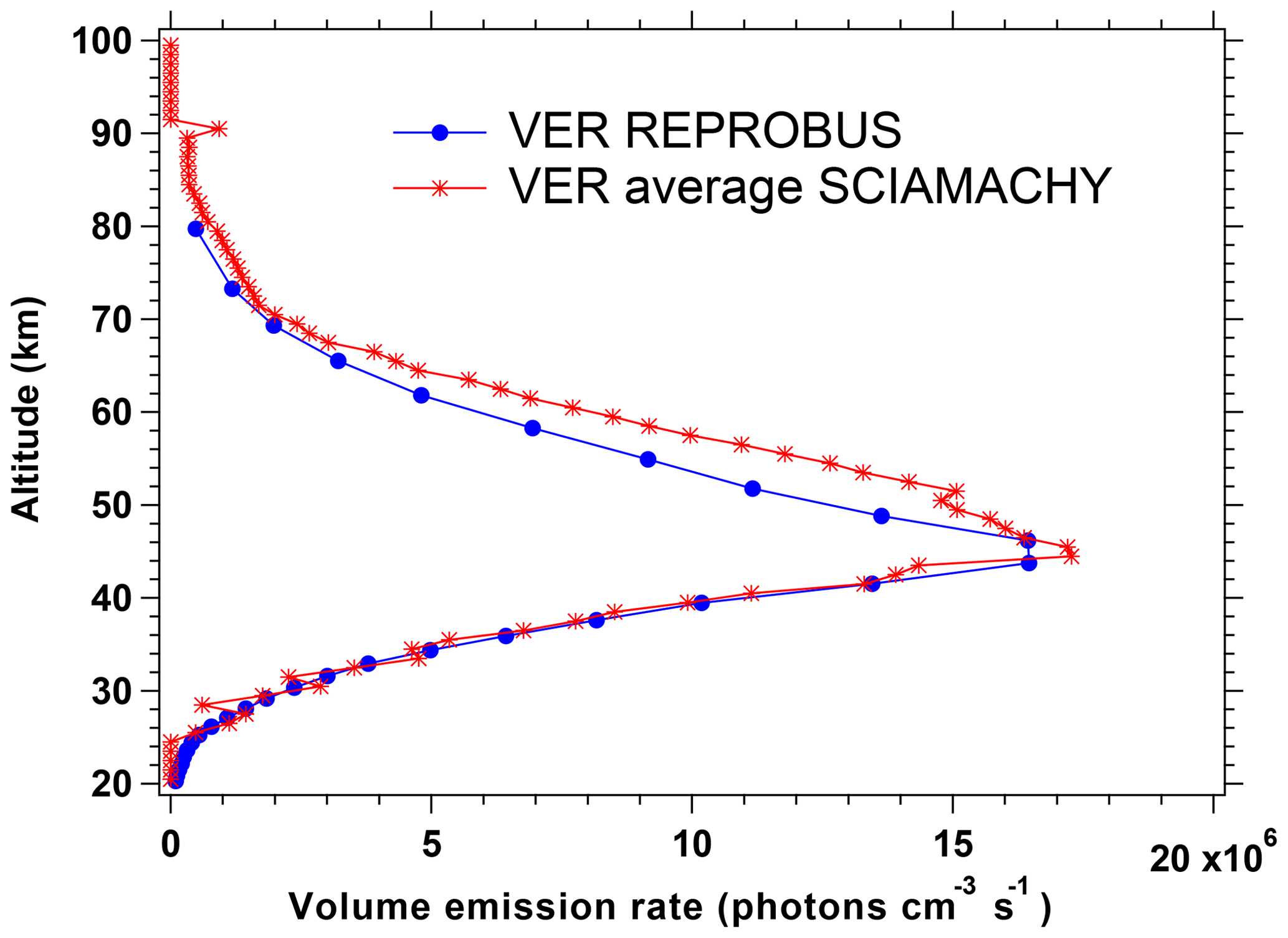
Figure D1 VER SCIAMACHY profile used to build the synthetic airglow spectrum put in the simulated spectrum to be inverted (red); associated (co-located) REPROBUS VER profile, showing the underestimation of REPROBUS airglow modelling above 50 km (blue). The airglow synthetic spectra associated with these two VER profiles are illustrated in Fig. D2. They are very similar.

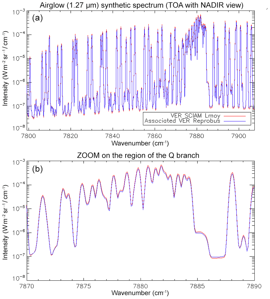
Figure D2 (a) Synthetic airglow spectra corresponding to the (red) SCIAMACHY VER profile of Fig. D1, (blue) associated REPROBUS VER profiles of Fig. D1. For the three tests, the red spectrum is put in the simulated data to invert. For test no. 1, it is also used as the Jacobian of the inverse model. For test no. 2, the blue spectrum is used as Jacobian of the inverse model (blue). The Jacobian spectra of test no. 3 are not represented here. (b) Zoom on the region of the Q branch.

The spectels contaminated by airglow are a source of bias on the Psurf retrieval. The more contaminated spectels we discard with a mask, the more this bias is expected to be reduced. However, at the same time, the more spectels we discard, the more we increase the random error since we lose some useful information on Psurf in the absorption bands. Thus, we are looking for a mask which provides a good compromise between bias and random error. Table D2 shows, however, that the spectel mask method does not allow meeting the MicroCarb requirement simultaneously in term of bias and random error using the MicroCarb B4 band only. Values are, however, not that far from MicroCarb requirements, and mask number no. 3, for example, allows being in spec in terms of bias (−0.04 hPa) while keeping a reasonable random error of 1.52 hPa. This method can thus be foreseen as a good alternative to the method no. 1 and is worth being tested on MicroCarb data when available.

Table D1 Results of the Psurf inversion by method no. 1 (airglow also inverted). Values printed in bold are non-compliant with MicroCarb requirement. Non-bold indicates compliant values.

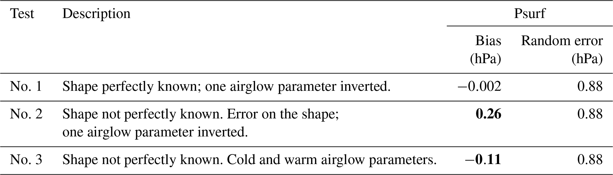
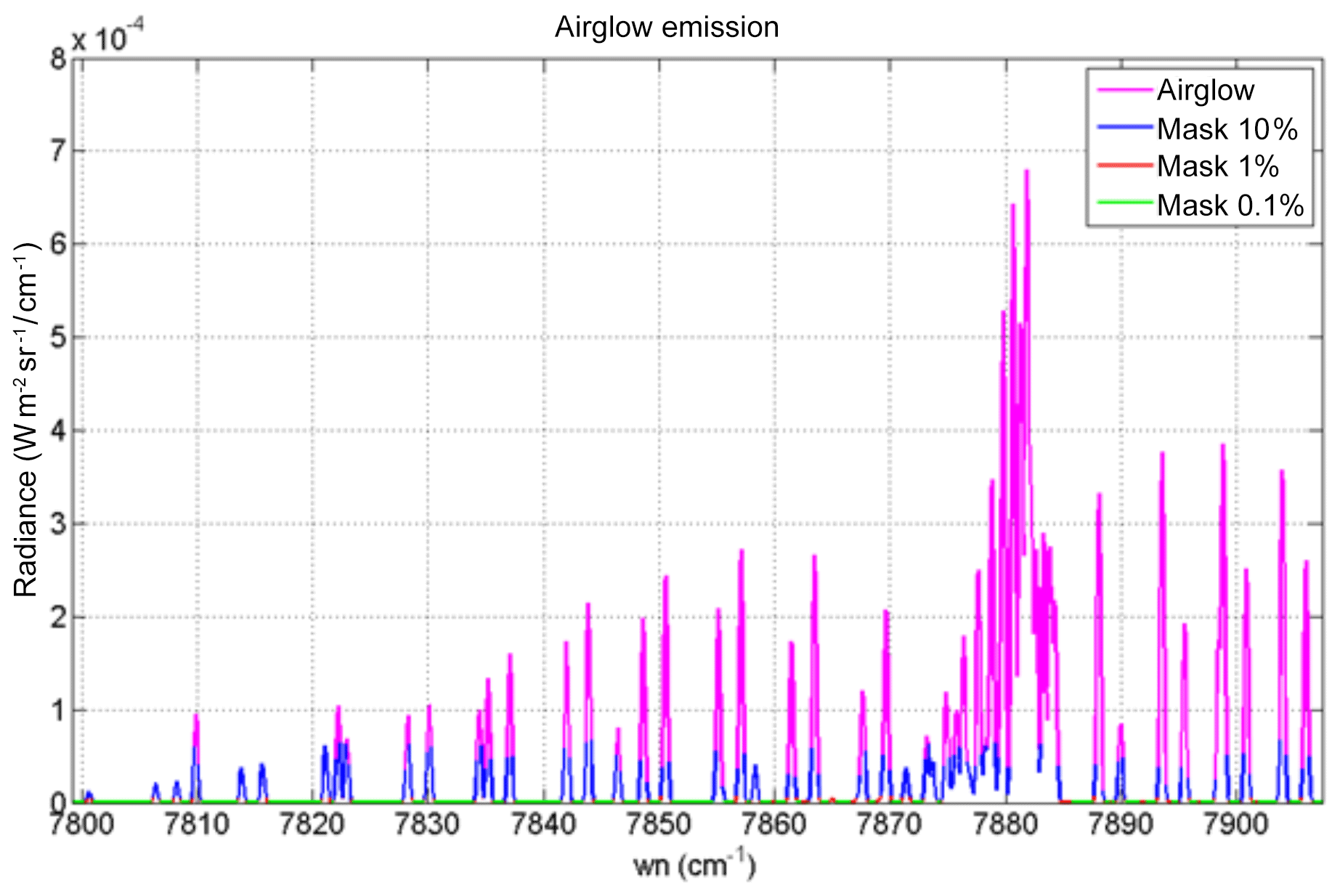
Figure D3 Airglow spectra at 1.27 µm, at MicroCarb resolution, used in our tests of inversion of Psurf with method no. 2 for several values of the spectel mask: no mask (pink), 10 % mask (blue), 1 % mask (red), and 0.1 % mask (green). The three masks remove, respectively, 14 %, 31 %, and 44 % of the spectels in the B4 band.

Table D2 Results of the inversion of Psurf in MicroCarb band B4 (1.27 µm) with method no. 2 (spectel mask). Values printed in bold are non-compliant with MicroCarb requirement. Non-bold indicates compliant values.

Appendix E: Contamination of absorption measurements by airglow emissions

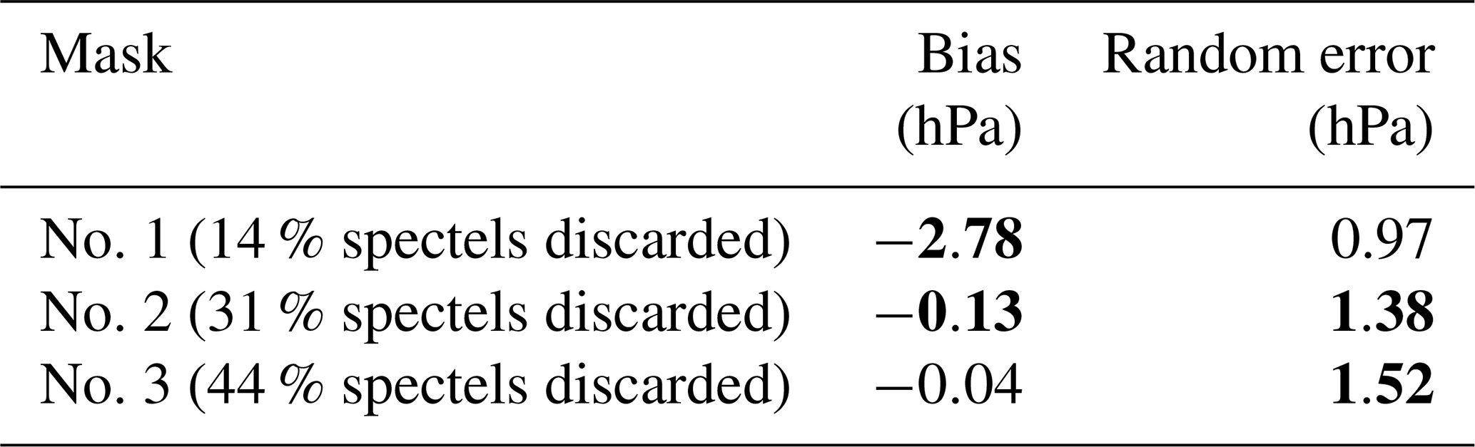
The contamination of the absorption O₂ band at 1.27 µm by the corresponding O₂^* airglow emission is an extreme case, in view of the strong intensity of the airglow (up to 40 megarayleigh). However, this particular band is not a unique case. In all nadir-viewing observations from space analysing scattered sunlight, the LOS goes across all the airglow layers (Fig. 1), and their emissions are superimposed on the scattered sunlight spectrum. We list below a few commonly used absorption bands and their potential contamination by airglow.

For the O₂ molecule (band A), Zarboo et al. (2018) retrieved the VER of the emission by the O₂ molecule excited in the ¹Σ state from SCIAMACHY limb observations when it decays to the fundamental in the A-band O₂ at 0.76 µm (their Fig. 5). One could estimate the nadir-viewing radiance from the total column. This is a contribution to radiance measurements in the A band, which (to our knowledge) has been ignored up to now, that should be subtracted systematically from any nadir A-band measurements, with its detailed spectral shape, before analysis. Sioris (2003) computed a synthetic spectrum of the A-band O₂ emission, including resonance scattering of solar photons. Then he performed a column O₂ retrieval, with and without the airglow contribution. In spite of the fact that the airglow may account for more than 10 % of the total radiance in the core of strong lines, the bias (negative) when neglecting to subtract the A-band airglow was found to be only 0.0061 % on the O₂ column retrieval. An independent study performed in the frame of the present work found −0.0073 %, confirming the Sioris estimate. However, both studies have assumed a total absence of this A-band emission below 50 km, while the corresponding VER profile derived from SCIAMACHY observations suggests a fast increase of the emission with decreasing altitude around 50 km (Fig. 5 of Zarboo et al., 2018). Not accounting for this A-band emission below 50 km will be more detrimental (for the accuracy of Psurf retrieval with A band) in low-albedo regions and low SZA values (resonance scattering penetrates more deeply at low SZA).

The CO₂ molecule illuminated by the Sun is subject to resonance fluorescence, with non-LTE emission in the bands where the absorption is measured (weak or strong CO₂ bands). This is to our knowledge not yet accounted for in GHG retrievals. In addition, there is a (0, 1) transition of the O₂(¹Δ) around 1.58 µm that interferes with a pair of CO₂ weak bands. Though this emission is about 50 times smaller than the 1.27 µm emission, it is preferable to use the other pair of CO₂ bands at 1.60 µm, as done by OCO-2 and MicroCarb instruments.

For the CH₄ molecule, Lopez-Puertas et al. (2005) reported limb observations of non-LTE emission of CH₄ in the thermal IR at 7.6 µm from Michelson Interferometer for Passive Atmospheric Sounding (MIPAS)/Envisat Fourier transform spectrometer (FTS) instrument. It began to be noticeable at 45 km altitude and represented up to 60 % of the emission at 70 km. Therefore, this non-LTE emission triggered by solar radiation forms an airglow layer that is intercepted in a nadir-viewing geometry. Such a known-to-exist contribution should be subtracted systematically from nadir-viewing measurements (i.e. Infrared Atmospheric Sounding Interferometer (IASI) measurements). This contribution has been ignored by de Wachter et al. (2017), analysing nadir IASI methane measurements. A rough estimate from figures of Lopez-Puertas et al. (2005) indicates a non-LTE horizontal emission of 100 nW cm⁻² sr⁻¹, over 4 cm⁻¹ at 50 km altitude. A vertical viewing would reduce this value by a Chapman factor of several tens, probably below the noise of IASI measurements (∼10 Nw (cm² sr cm⁻¹)⁻¹. However, it should be noted that there is also certainly some non-LTE emission below 50 km (difficult to see for MIPAS), and that this spectrum has a very similar shape as the LTE emission. Therefore, the non-LTE emission should be modelled, scaled to MIPAS determinations at high altitudes, and subtracted blindly form nadir viewing (IASI-type measurements). It is possible that other bands of CH₄ used for GHG retrievals may be similarly affected.

The fluorescence of H₂O molecule excited by solar radiation has been observed at 2.67 µm in the coma of several comets (i.e. Bockelée-Morvan et al., 2015) and should be present in the atmosphere of the Earth, as well as in the other lines which are present in GHG bands (i.e. at 2.0 µm). These H₂O airglow emissions superimposed to surface radiation have not been subtracted from nadir observations or their intensity even estimated, to the best of our knowledge.

The fluorescence of CO molecule excited by solar radiation has been observed at 4.53 µm in the upper atmosphere of Venus with high spectral resolving power (R∼43 000) by Marcq et al. (2015). The same must happen in the atmosphere of the Earth; introducing a bias of about 1 % on the CO column retrieval (rough estimate) may not be so important because it is well below the currently achieved accuracy of some tens of percent on CO columns.

Appendix F: Processing of SCIAMACHY level-1c radiance data

Here, we show some figures describing our processing of level-1c SCIAMACHY radiance data, as explained in Sect. 3.1, in order to get a “pure” radiance spectrum of the O₂^* airglow. We also show in Fig. F5 a typical distribution along one orbit of the SCIAMACHY limb observations used in our analysis.

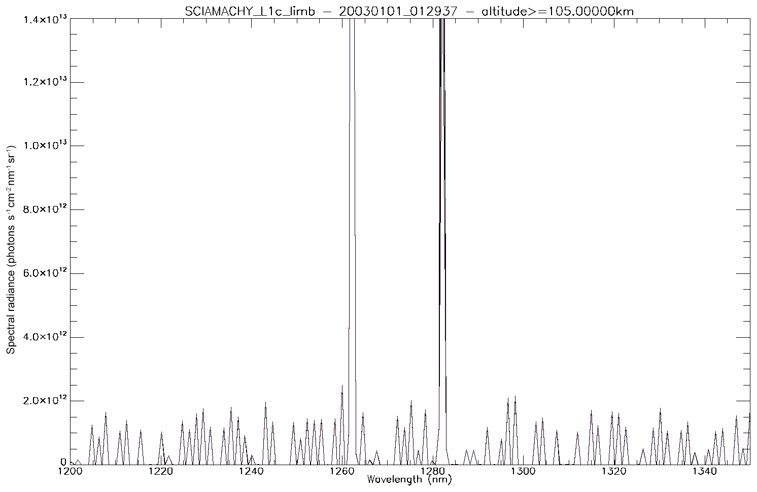
Figure F1 This high-altitude spectrum recorded above 105 km contains some residual spectral (readout) patterns left from the calibration step and is subtracted from all measurements obtained at lower altitude in the same scan limb.

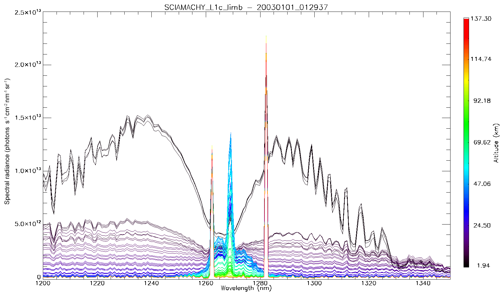
Figure F2 Spectra corrected from the high-altitude spectrum still showing two bad pixels at wavelength 1262.267 and 1282.128 nm. We replaced their value by the average of their two surrounding pixels to obtain spectra of Fig. F3. The tangent altitude of the LOS is colour coding each spectrum.

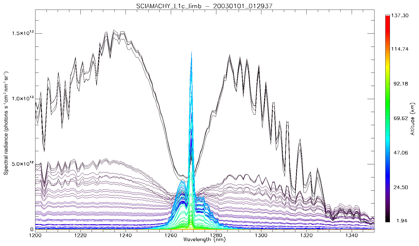
Figure F3 Same as Fig. F2, after correction of the two bad pixels. In addition to the O₂^* airglow, there is the radiance of solar light scattered by air and aerosols, increasing when tangent altitude is decreasing. The strong absorption of O₂ in the 1.27 µm band becomes obvious at the lowest altitudes.

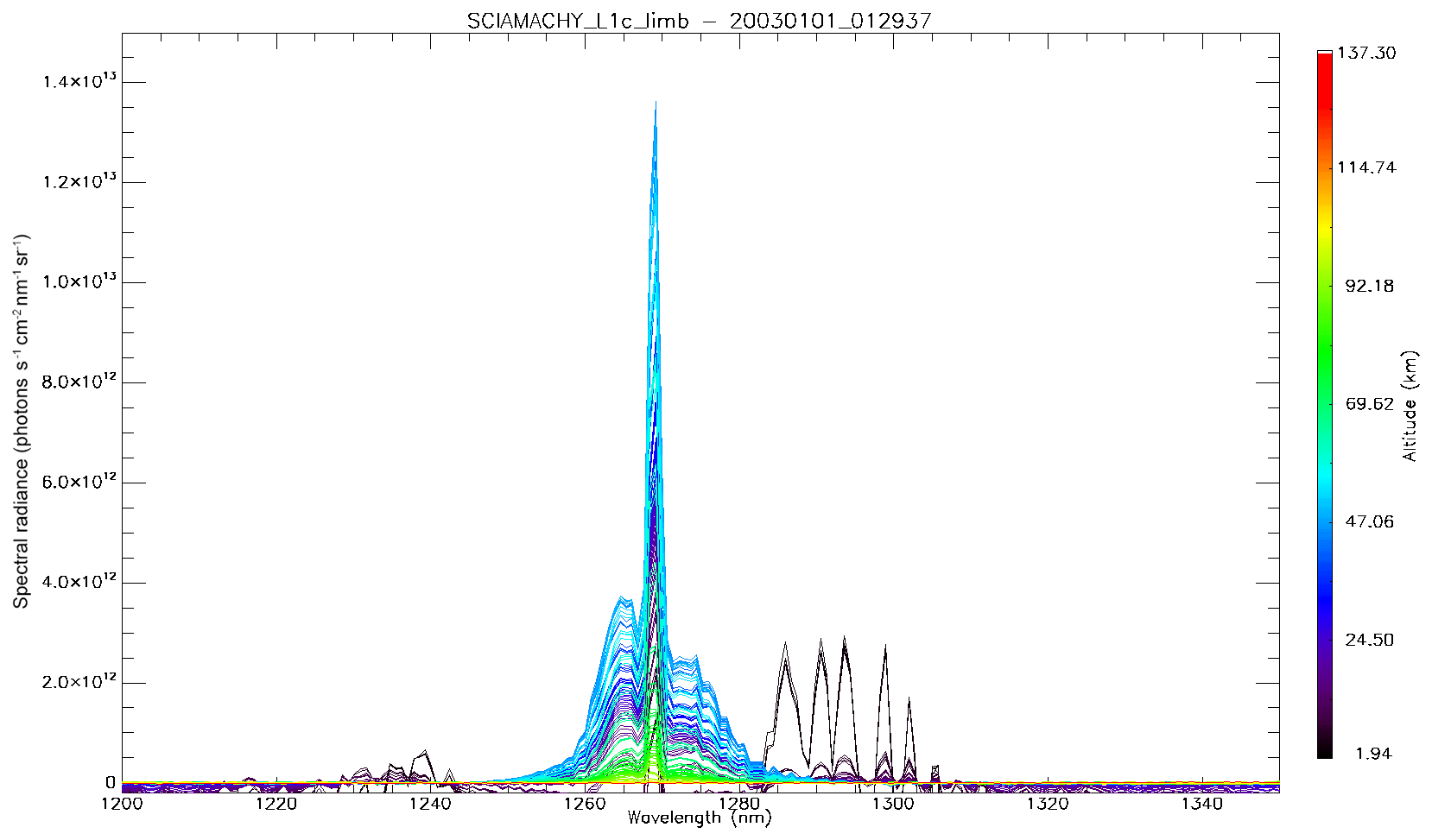
Figure F4 Airglow spectra obtained from Fig. F3 by subtracting a linear interpolation based on the two constant values of the continuum (one on each side) estimated from the median value of all points outside the O₂^* band. This correction is valid above ∼20 km tangent altitude.

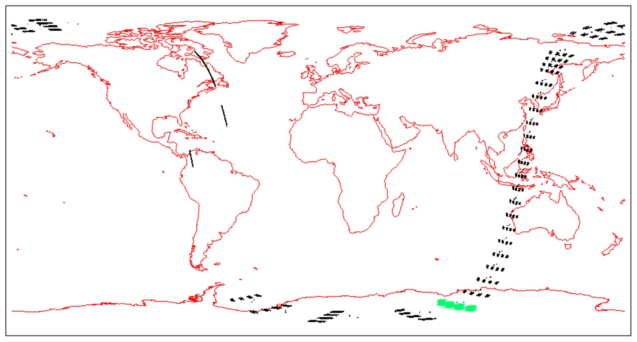
Figure F5 Geographic positions of SCIAMACHY LOS tangent points at the limb (by groups of four) for Envisat orbit no. 25293, starting on 1 January 2007 at 01:12 UT. The green points are the locations of the limb spectra which are compared with our theoretical derivation in Sect. 3.