the Creative Commons Attribution 4.0 License.
the Creative Commons Attribution 4.0 License.
 | 13 Jul 2020
Instrumental characteristics and potential greenhouse gas measurement capabilities of the Compact High-Spectral-Resolution Infrared Spectrometer: CHRIS
Marie-Thérèse El Kattar
Frédérique Auriol
Hervé Herbin
Ground-based high-spectral-resolution infrared measurements are an efficient way to obtain accurate tropospheric abundances of different gaseous species, in particular greenhouse gases (GHGs) such as CO2 and CH4. Many ground-based spectrometers are used in the NDACC and TCCON networks to validate the Level 2 satellite data, but their large dimensions and heavy mass make them inadequate for field campaigns. To overcome these problems, the use of portable spectrometers was recently investigated. In this context, this paper deals with the CHRIS (Compact High-Spectral-Resolution Infrared Spectrometer) prototype with unique characteristics such as its high spectral resolution (0.135 cm−1 nonapodized) and its wide spectral range (680 to 5200 cm−1). Its main objective is the characterization of gases and aerosols in the thermal and shortwave infrared regions. That is why it requires high radiometric precision and accuracy, which are achieved by performing spectral and radiometric calibrations that are described in this paper. Furthermore, CHRIS's capabilities to retrieve vertical CO2 and CH4 profiles are presented through a complete information content analysis, a channel selection and an error budget estimation in the attempt to join ongoing campaigns such as MAGIC (Monitoring of Atmospheric composition and Greenhouse gases through multi-Instruments Campaigns) to monitor GHGs and validate the actual and future space missions such as IASI-NG and Microcarb.
- Article
(3610 KB) - Full-text XML
- BibTeX
- EndNote


Remote-sensing techniques have gained a lot of popularity in the past few decades due to the increasing need of continuous monitoring of the atmosphere (Persky, 1995). Greenhouse gases and trace gases as well as clouds and aerosols are detected and retrieved, thus improving our understanding of the chemistry, physics and dynamics of the atmosphere. Global-scale observations are achieved using satellites, and one major technique is infrared high-spectral-resolution spectroscopy (IRHSR). This technique offers radiometrically precise observations at high spectral resolution (Revercomb et al., 1988) where quality measurements of absorption spectra are obtained. TANSO-FTS (Suto et al., 2006), IASI (Clerbaux et al., 2007) and AIRS (Aumann et al., 2003) are examples of satellite sounders covering the thermal infrared (TIR) region. The observations acquired from such satellites have many advantages: day and night data acquisition, possibility to measure concentrations of different gases, the ability to cover land and sea surfaces (Herbin et al., 2013a), and the added characteristic of being highly sensitive to various types of aerosol (Clarisse et al., 2010). These spectrometers also have some disadvantages: local observations are challenging to achieve due to the pixel size that limits the spatial resolution, and the sensitivity in the low atmospheric layers, where many short-lived gaseous species are emitted but rarely detected, is weak.
To fill these gaps, ground-based instruments are used as a complementary technique, and one famous high-precision Fourier-transform spectrometer is the IFS125HR from Bruker™, which is briefly discussed in Sect. 3.5 (further details can be found in Wunch et al., 2011). More than 30 instruments are currently deployed all over the world in two major international networks: TCCON (https://tccondata.org/, last access: 22 June 2020) and NDACC (https://www.ndsc.ncep.noaa.gov/, last access: 22 June 2020). This particular instrument has a very large size ( m) and a mass well beyond 100 kg, therefore achieving a long optical path difference and leading to a very high spectral resolution (0.02 and cm−1 for TCCON and NDACC, respectively). Despite its outstanding capabilities, this spectrometer is not suitable for field campaigns, so it is mainly used to validate Level 2 satellite data, thus limiting the scientifically important ground-based extension of atmospheric measurement around the world.
One alternative is the new IFS125M from Bruker (Pathatoki et al., 2019), which is the mobile version of the well-established IFS125HR spectrometer. This spectrometer provides the highest resolution available for a commercial mobile Fourier-transform infrared (FTIR) spectrometer, but it still has a length of about 2 m and requires on-site realignment by qualified personnel. Another alternative is the use of several compact medium- to low-resolution instruments that are currently under investigation, such as a grating spectrometer (0.16 cm−1), a fiber Fabry–Pérot interferometer (both setups presented in Kobayashi et al., 2010) and the IFS66 from Bruker (0.11 cm−1) described in Petri et al. (2012). The EM27/SUN is the first instrument to offer a compact, optically stable, transportable spectrometer (Gisi et al., 2012) with a high signal-to-noise ratio (SNR) and that operates in the SWIR (short-wavelength infrared) region. A new prototype called CHRIS (Compact High-Spectral-Resolution Infrared Spectrometer) was conceived to satisfy some very specific characteristics: high spectral resolution (0.135 cm−1, better than TANSO-FTS and the future IASI-NG) and a large spectral band (680–5200 cm−1) to cover the current and future infrared satellite spectral range and optimize the quantity of the measured species. Furthermore, this prototype is transportable and can be operated for several hours by battery (>12 h), so it is suitable for field campaigns. The full presentation of the characteristics and the calibration of this instrumental prototype is presented in Sect. 2.
Since carbon dioxide (CO2) and methane (CH4) are the two main greenhouse gases emitted by human activities, multiple campaigns have been launched, such as the MAGIC (Monitoring of Atmospheric composition and Greenhouse gases through multi-Instruments Campaigns) initiative, to better understand the vertical exchange of these greenhouse gases (GHGs) along the atmospheric column and to contribute to the preparation and validation of future space missions dedicated to GHG monitoring. CHRIS is part of this ongoing mission, and this work presents for the first time the capabilities of such a setup in achieving GHG measurements. Analysis of the forward model, state vector and errors is explained in Sect. 3.
In this context, we present in Sect. 3.5 a complete information content study for the retrieval of CO2 and CH4 of two other ground-based instruments that also participated in the MAGIC campaign: a comparison study with the IFS125HR instrument and, since CHRIS and the EM27/SUN have a common band in the SWIR region, a study to investigate the spectral synergy in order to quantify the complementary aspects of the TIR–SWIR–NIR (NIR stands for near-infrared) coupling for these two instruments. Moreover, Sect. 4 describes the channel selection made in this study. Finally, we summarize our results and perspectives for future applications, in particular the retrieval of GHGs in the MAGIC framework.
CHRIS is an instrumental prototype built by Bruker™ and used in different domains of atmospheric optics. Its recorded spectra contain signatures of various atmospheric constituents such as GHGs (H2O, CO2, CH4) and trace gases. The capacity to measure these species from a technical point of view as well as the characterization of this prototype in terms of spectral and radiometric calibrations is presented in the following subsections.
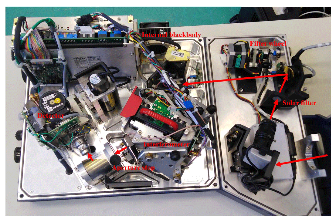
Figure 1An internal look at CHRIS. The red arrows illustrate the optical path of the solar beam inside the spectrometer.
2.1 General characteristics
CHRIS is a portable instrumental prototype with a mass of approximately 40 kg and dimensions of cm, making it easy to operate in the field. The tracker, which is similar to the one installed on the EM27/SUN and described in detail in Gisi et al. (2012), leads the solar radiation through multiple reflections on the mirrors to a wedged fused-silica window.
An internal look at CHRIS is shown in Fig. 1, where the optical path of the solar beam is represented with red arrows: after multiple reflections on the tracker's mirrors, the solar radiation enters the spectrometer through the opening and is then reflected by the first mirror, where the charge-coupled device (CCD) camera verifies the collimation of the beam on the second mirror, which has a solar filter. At this level, CHRIS has a filter wheel that can be equipped with up to five optical filters with a diameter of 25 mm. Filters are widely used when making solar measurements to reduce noise and nonlinearity effects. After reflection on the second mirror, the beam enters the RockSolid™ Michelson interferometer, which has two cube-corner mirrors to ensure the optical alignment stability of the beam and a KBr beam splitter. After that, the radiation is blocked by an adjustable aperture stop, which can be set to between 1 and 18 mm. This limits the parallel beam parameter and can be used to reduce the intensity of the incoming sunlight in case of saturation of the detector. The remaining radiation falls onto an MCT (mercury cadmium telluride) detector; then it is digitized to obtain the solar absorption spectra in arbitrary units. This detector uses a closed-cycle Stirling cooling system (a.k.a. cryocooler), so no liquid nitrogen has to be used. As the vibrations of the compressor may introduce noise in the spectra (see Sect. 2.6), a high scanning velocity (120 KHz) is needed.
A standard nonstabilized He–Ne laser controls the sampling of the interferogram. The condensation of the warm, humid air on the beam splitter due to its transportation between cold and warm environments is the main reason a dessicant cartridge is used, so the spectrometer can operate under various environmental conditions. CHRIS also has an internal blackbody, which can be heated up to 353 K to make sure that there is no drift in the TIR region, and it also serves as an optical source to regularly verify the response of the detector.
2.2 Measurements and analysis
CHRIS's method of data acquisition is explained as follows: the interferograms are sampled and digitized by an analog-to-digital converter (ADC) and then numerically resampled at constant intervals of optical path difference (OPD) by a He–Ne reference laser signal controlled by the aperture stop diameter. In order to determine a suitable compromise between the latter and to avoid the saturation of the signal, measurements must be done in a clear (no clouds or aerosols) and nonpolluted (no gases with high chemical reactivity) atmosphere. For this purpose, a field campaign was carried out at El Observatorio Atmosférico de Izaña (28.30∘ N, 16.48∘ W) on the island of Tenerife. This particular observatory site is high in altitude (2374 m), away from pollution sites and has an IFS125HR listed in both the NDACC and TCCON networks. Saturation of CHRIS's detector is reached at a value of 32 000 ADC. The MCT detector is known for its high photometric accuracy, but it also exhibits a nonlinear response with regard to the energy flux in cases of high incident energy. This led us to choose an aperture stop of 5 mm, which is the best compromise between saturation and incoming energy flux.
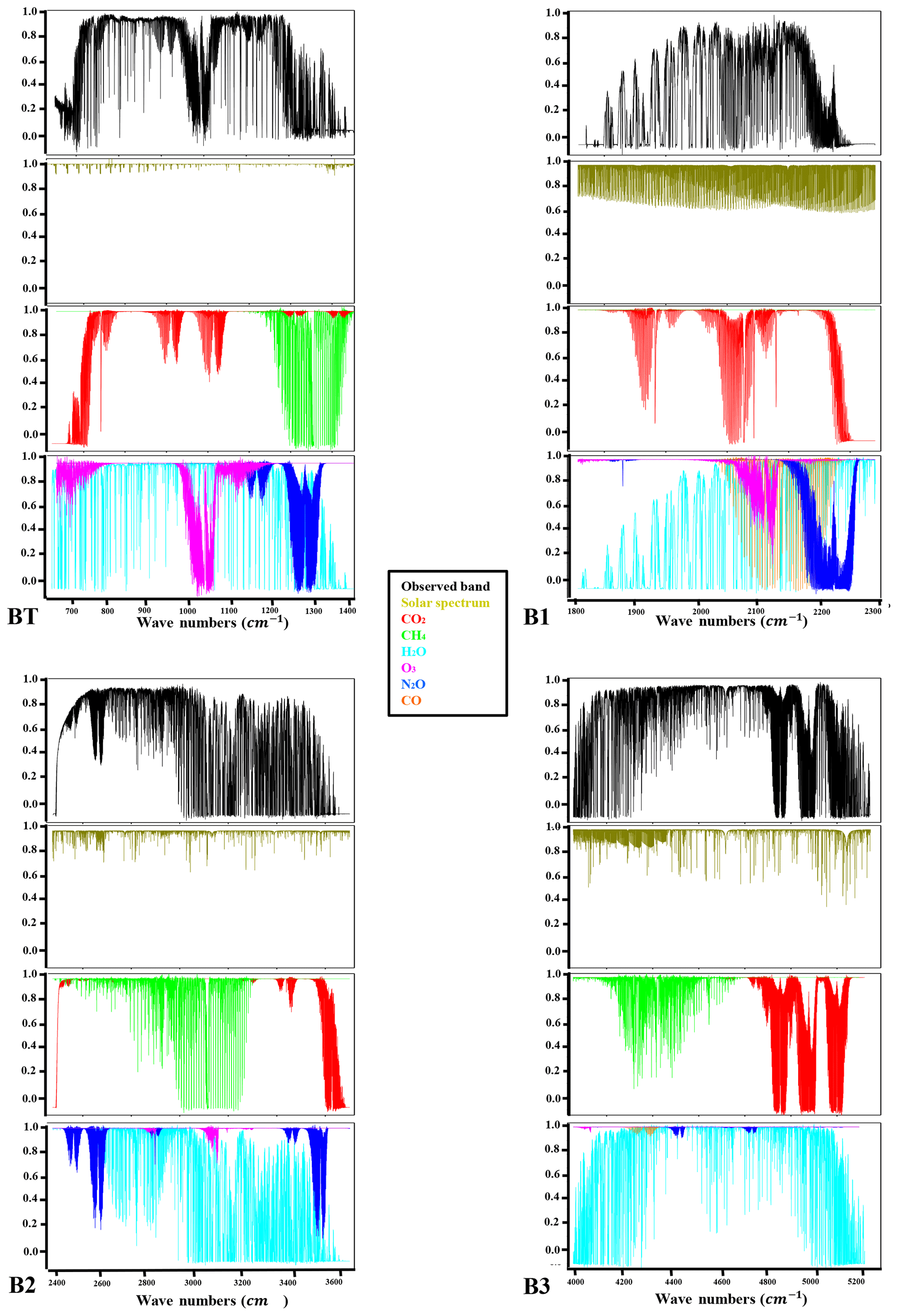
Each spectrum corresponds to the solar transmission light in the total atmospheric column in a field of view (FOV) of 0.006 mrad. The spectral range spans the region from 680 to 5200 cm−1 (1.9 to 14.7 µm), which corresponds to the middle-infrared region (MIR). The water vapor causes the saturation we see between the bands, thereby explaining the zero signal. Therefore, we divided the spectrum into four distinctive spectral bands presented in Table 3: TB (thermal band; 680–1250 cm−1), B1 (1800–2300 cm−1), B2 (2400–3600 cm−1) and B3 (3900–5200 cm−1). This annotation is used for the rest of the paper.
2.3 Optical features
A technical study was conducted on this prototype in order to evaluate its optical and technical properties with a constant aperture stop diameter of 5 mm. One of the most important findings is the effect of the number of scans on the measured spectra. In practice, a scan is the acquisition of a single interferogram when the mobile mirror of the Michelson interferometer begins data collection at the zero path difference (ZPD) and finishes at the maximum length, therefore achieving the highest resolution required. In Fig. 2, the spectrum with 10 scans has a higher amplitude than those with 50 and 100 scans. On the other hand, the spectra with 50 and 100 scans are clearly less noisy than that with 10 scans. This is due to the fact that the increase in the number of scans causes an increase in the SNR, which leads to a decrease in noise. However, there is a limit to the number of scans beyond which no improvement of the SNR is obtained. The SNR is proportional to the square root of the acquisition time (number of scans), also known as Fellgett's advantage, and since the detector is dominated by shot noise, the improvement of the SNR with the number of scans is blocked at a certain value. This is why the spectra of 100 and 200 scans do not show a significant difference. The SNR is an estimation of the root-mean-squared noise of the covered spectral domain and can be calculated in OPUS (the running program for CHRIS) using the function SNR with the “fit parabola” option; it is estimated to be approximately 780. An optimized criterion is chosen to select the appropriate number of scans: when the wanted species has a fast-changing concentration, such as volcanic plumes, a relatively small number of scans is needed to be able to follow the change in the atmospheric composition temporally. In contrast, when measurements of relatively stable atmospheric composition are made, for example GHGs (CO2 and CH4), the number of scans can be increased to 100. For instance, the time needed for one scan with a scanning velocity of 120 KHz is 0.83 s, so 100 scans take approximately 83 s, which is low in comparison to the variability of CO2 and CH4 in the atmosphere.
Another important feature is the effect of the gain amplitude (and preamplifiers, which amplify the signal before digitization) on the spectra. Those parameters should be chosen in a way that the numeric count falls in a region where no detector saturation occurs. If the gain is increased by a certain amount, the background noise is increased by the same amount. The use of such an option in the measurement procedure might be considered in cases where the signal is very weak, like lunar measurements. Note that there are other ways to increase the intensity of the signal, like using signal amplifying filters (see Sect. 2.1) or increasing the aperture stop diameter.
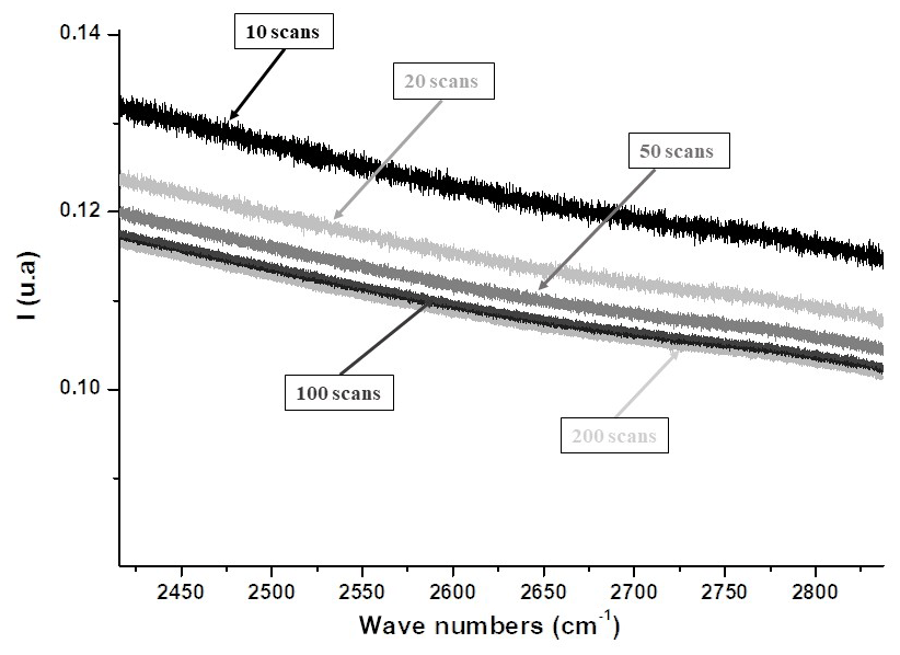
Figure 2Improvement of the SNR with different scan numbers and a fixed scan speed of 120 KHz.
2.4 Radiometric and spectral calibration
In the following section, the spectral and radiometric calibrations are discussed in order to convert spectra from numeric counts (expressed in arbitrary units) to radiance ().
2.4.1 Radiometric calibration
Despite the fact that CHRIS has an internal blackbody, radiometric calibration cannot be overlooked because of its narrow spectral coverage (only the TIR region), and since the radiometric noise and the time- and wavelength-dependent calibration errors are magnified in the inversion process, high radiometric precision is required to derive atmospheric parameters from a spectrum. We calibrate our spectra using the two-point calibration method explained in Revercomb et al. (1988). This method consists of using the observations of hot and cold blackbody reference sources, which will be used as the basis for the two-point calibration at each wave number. A cavity blackbody was acquired by the LOA (Laboratoire d'Optique Atmosphérique) to perform regular radiometric calibrations. The latter is an HGH/RCN1250N2, certified by the LNE (Laboratoire National de métrologie et d'Essais) as having an emissivity greater than 0.99 in the spectral domain spanned by CHRIS, a stability of 0.1 at 1173 K and an opening diameter of up to 50 mm (corresponding to that of CHRIS) and as covering temperatures from 323 to 1523 K. This cavity blackbody is mounted on an optical bench and used before and after each campaign to perform absolute radiometric calibrations through open-path measurements and to make sure that this calibration is stable across the whole spectral range. These two blackbody temperatures are viewed to determine the slope m and offset b (Eqs. 1 and 2), which define the linear instrument response at each wave number. The slope and the offset can be written following Revercomb et al. (1988):
where S is the blackbody spectrum recorded, and Bν corresponds to the calculated Planck blackbody radiance. The subscripts h and c correspond to the hot (1473 K) and cold (1273 K) blackbody temperatures, respectively. Finally, the calibrated spectrum expressed in watts per square meter steradian centimeter is obtained by applying the following formula:
where S is the spectrum recorded by CHRIS.
2.4.2 Instrumental line shape and spectral calibration
One open-path measurement using the calibrated HGH blackbody as source was performed, similar to the one previously described in Wiacek et al. (2007), to record a spectrum without applying any apodization. Our colleagues in the PC2A laboratory provided us with a 10 cm long cell with a free diameter of 5 cm, where the pressure inside is monitored by a capacitive gauge. With the help of the line-by-line radiative transfer algorithm ARAHMIS (atmospheric radiation algorithm for high-spectral measurements from infrared spectrometer) developed at the LOA laboratory, a maximum optical path difference (MOPD) of 4.42 cm was determined, corresponding to a spectral resolution of 0.135 cm−1 using a sinc function with a spectral sampling every 0.06025 cm−1 to satisfy the Nyquist criterion. In FTIR spectroscopy, a poor instrumental line shape (ILS) determination generates a significant error in the retrieval process, so we are currently modifying the optical bench in order to perform an ILS determination at the same time as the radiometric and spectral calibrations before each field campaign.
The sampling of the interferogram is controlled by a standard, non-frequency-stabilized He–Ne laser with a wavelength of 632.8 nm, which serves as a reference while converting from the distance scale to the wave number scale. The instrument is subjected to changes in pressure and temperature since it operates in different locations and therefore under different meteorological conditions. This will cause a change in the refractive index and as a consequence a change in the reference wavelength of the laser, which will lead to an instability in the conversion process and therefore the need for a spectral calibration to reduce this error. The ILS line defined above is used to resimulate isolated absorption lines from the high-resolution transmission molecular absorption (HITRAN) database (Gordon et al., 2017) considering nonapodized spectra, which allows the exploitation of the full spectral resolution. In short, we choose an intense unsaturated H2O absorption line that is always present in the spectra; then we compare the central wave number (ν) with the calculated one (ν*) following the equation
where α is the calibration factor. Equation (4) is limited by a precision of 0.038 cm−1, corresponding to roughly half of the spectral sampling, estimated from the standard deviation between the theoretical HITRAN spectroscopic lines and the measured ones by CHRIS. Figure 3 shows the comparison between a calibrated and a noncalibrated spectrum along with the solar Planck function explained in Sect. 3.1. The spectral and radiometric calibration procedure is automated using a MATLAB code to convert the spectra instantly from numeric counts to absolute radiance.
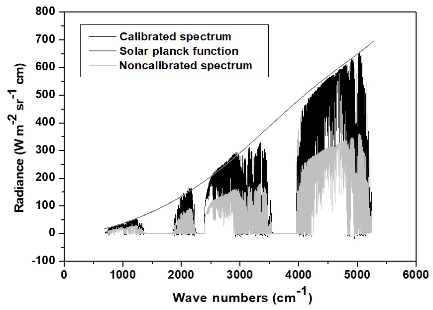
Figure 3The calibration process transforms the noncalibrated spectrum (light gray) into a calibrated one (black) that fits with the solar Planck function (solid gray line).
2.5 Radiometric stability
During campaigns and after long transportation, constant measurement of the internal blackbody, which can be heated up to 353 K, is carried out in the thermal infrared region (most affected by drifts). Figure 4 shows the variations of the internal blackbody during multiple field campaigns: a little fluctuation in function of the measurement conditions can be seen, but depending on the locations and even years, no systematic drift can be detected, so we can safely say that the instrument is quite stable between each laboratory calibration.
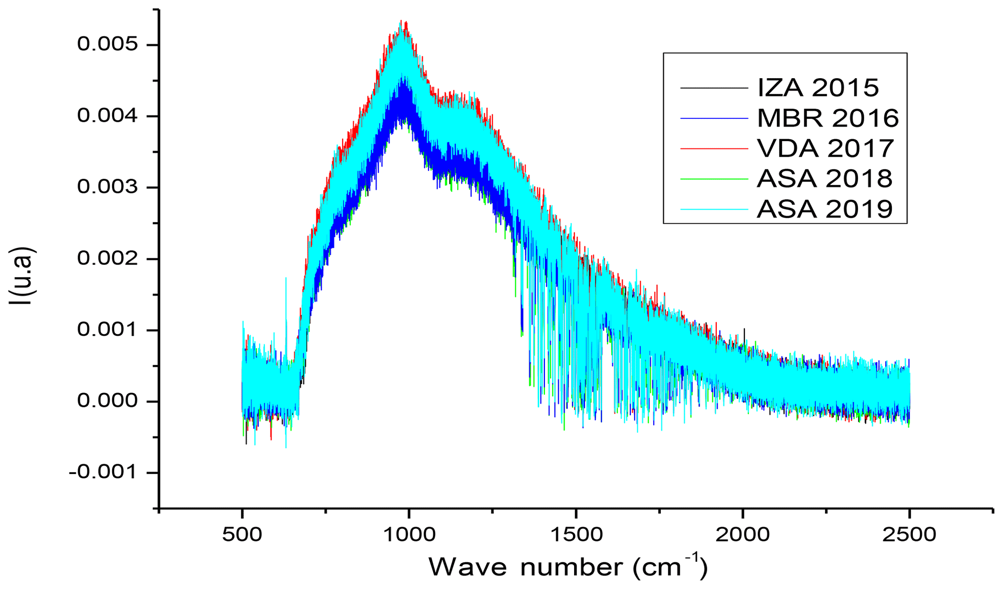
Figure 4The radiometric stability of the instrument is achieved by following the variations of the internal blackbody during multiple field campaigns. IZA: Izana; MBR: M'Bour; VDA: Villeneuve d'Ascq; ASA: Aire-sur-l'Adour.
2.6 Spectral artifacts
There are commonly several well-known spectral artifacts: aliasing, the picket fence effect (also known as the resolution bias error) and phase correction. These are well controlled in CHRIS.
Aliasing is the result of the missampling of the interferogram at the x-axis locations, which leads to errors in the retrieved column abundances due to its overlap with the original spectrum. The He–Ne laser, having a wavelength λ of 632.8 nm, generates the sampling positions of the interferogram at each zero crossing. No overlap will occur if the signal of the spectrum is zero above a maximum wave number νmax and if νmax is smaller than the folding wave number . Since Δν is related to the sample spacing Δx, the minimum possible Δx is 1∕31 600 cm since each zero crossing occurs every λ∕2. This corresponds to a folding wave number of 15 800 cm−1, i.e., the maximum bandwidth that can be measured without overlap has a width of 15 800 cm−1. This source error is of special relevance to the spectra acquired in the near-infrared region. However, for the MIR, the investigated bandwidth is much smaller than 15 800 cm−1, where νmax is less than 5200 cm−1, so CHRIS's spectra are not affected by this problem (Dohe et al., 2013).
The picket fence effect, or the resolution bias error, becomes evident when the interferogram contains frequencies that do not coincide with the frequency sample points, but this is overcome in our spectra by the classical method of the zero filling factor (ZFF), where zeros are added to the end of the interferogram before the Fourier transform is performed, thereby doubling the size of the original interferogram.
Phase correction is necessary while converting the interferogram into a spectrum, which is relevant to single-sided measurements, similar to those acquired by CHRIS. Mertz phase correction is the method used for CHRIS to overcome this problem; it relies on extracting the real part of the spectrum from the complex output by multiplication of the latter by the inverse of the phase exponential, therefore eliminating the complex part of the spectrum generated.
Besides these classical FTIR artefacts, we noticed during our tests that when using a scan speed of 160 KHz, we drastically increase the nonlinearity effect of the detector (see Fig. 5). However, we identified a ghost signal for low scanning velocities (for example 40 KHz as shown in Fig. 6). This ghost is specific to CHRIS because it is caused by the noise introduced from the vibrations of the compressor used in the closed-cycle Stirling cooler as mentioned in Sect. 2.1. The choice of a scanning velocity of 120 KHz is a compromise between two important features: the elimination of the ghost signal, which appears at scanner velocities below 80 KHz, and the increase in the detector nonlinearity at a velocity of 160 KHz.
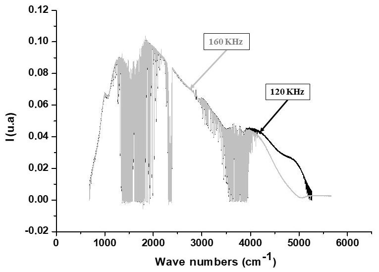
Figure 5Spectra of the external blackbody with two different scanning velocities: 120 KHz (black) and 160 KHz (light gray).
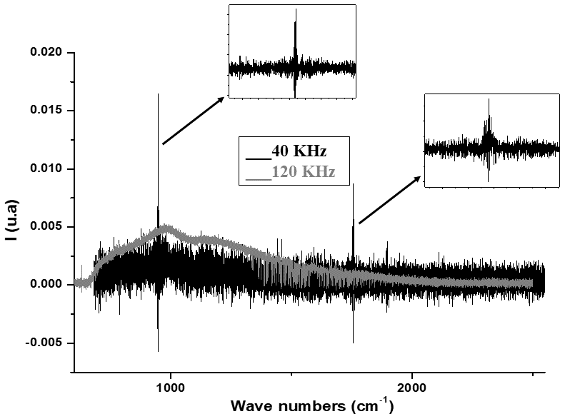
Figure 6Spectra of the internal blackbody of CHRIS with scanner velocities of 40 KHz (black) and 120 KHz (light gray).
Since CHRIS is an instrumental prototype, its ability to retrieve GHGs is unknown; therefore it is important to perform an information content study to quantify its potential capability to retrieve GHGs as a first attempt. In this context, CHRIS is one of the instruments deployed in the MAGIC project alongside satellites, lidar, balloons and ground-based measurements. MAGIC is a French initiative supported by the CNES (Centre National d'Etudes Spatiales), which aims to implement and organize regular annual campaigns in order to better understand the vertical exchange of GHGs (CO2 and CH4) along the atmospheric column and establish a long-term validation plan for the satellite Level 2 products.
3.1 The forward model
Accurate calculations of the radiances observed by CHRIS are achieved with the line-by-line radiative transfer algorithm ARAHMIS over the thermal and shortwave infrared spectral range (1.9–14.7 µm). Gaseous absorption is calculated based on the updated HITRAN 2016 database (Gordon et al., 2017). The absorption lines are computed assuming a sinc line shape, and no apodization is applied, which allows the exploitation of the full spectral resolution. In this study, the term “all bands” refers to the use of the CHRIS bands TB, B1, B2 and B3 simultaneously (see Sect. 2.2). Absorption continua for H2O and CO2 are also included from the Mlawer–Tobin–Clough–Kneizys–Davies (MT-CKD) model (Clough et al., 2005). The pseudotransmittance spectra corresponding to direct sunlight from the center of the solar disk reported by Toon (2015) is used as the incident solar spectrum interpolated on the spectral grid of CHRIS. The effective brightness temperature depends strongly on the wave number; thus the Planck function is calculated in each spectral domain of CHRIS determined from Trishchenko (2006), who combined the work of four recent solar reference spectra. Two of these reference spectra with 0.1 % relative difference are taken into consideration and then adjusted by a polynomial fit (solid line in Fig. 3). In the gaseous retrieval process, the spectrometer's line of sight (LOS) has to be known for calculating the spectral absorption of the solar radiation while passing through the atmosphere. For this, the time and the duration of each measurement are saved, from which the required effective solar elevation (and the solar zenith angle, SZA) is calculated based on the routine explained in Michalsky (1988).
As mentioned in Sect. 3.3.2, Izaña offers clear nonpolluted measurements since it is high in altitude and away from major pollution sites, so calculations are performed based on the concentration of the desired atmospheric profile with the corresponding profile information: the temperature, pressure and relative humidity are derived from the radiosondes (http://weather.uwyo.edu/upperair/sounding.html); CO2 and CH4 profiles are derived from the TCCON database, whereas O3, N2O and CO concentrations are calculated from a typical midlatitude summer profile. Figure 7 shows the results of the forward model simulation superimposed with the four infrared bands measured by CHRIS. For each band, we present the influence of the solar spectrum, the GHGs (CO2 and CH4) and the major interfering molecular absorbers. We can see good agreement between the ARAHMIS simulations and the CHRIS measurements under clear sky conditions.
3.2 Information content theoretical basis
Once the forward model is calculated, we rely on the formalism of Rodgers (2000) that introduces the optimal estimation theory used for the retrieval, which is widely described elsewhere (e.g., Herbin et al., 2013a) and summarized hereafter.
In the case of an atmosphere divided into discrete layers, the forward radiative transfer equation gives an analytical relationship between the set of observations y (in this case the radiance) and the vector of true atmospheric parameters x (i.e., the variables to be retrieved: vertical concentration profiles of CO2 and/or CH4):
where F is the forward radiative transfer function (here the ARAHMIS code), b represents the fixed parameters affecting the measurement (e.g., atmospheric temperature, interfering species, viewing angle), and ε is the measurement error vector.
In the following information content study, two matrices fully characterize the information provided by CHRIS: the averaging kernel A and the total error covariance Sx.
The averaging kernel matrix A gives a measurement of the sensitivity of the retrieved state to the true state and is defined by
where K is the Jacobian matrix (also known as the weighting function). The ith row contains the partial derivatives of the ith measurement with respect to each (j) element of the state vector , and KT is its transpose.
The gain matrix G, whose rows are the derivatives of the retrieved state with respect to the spectral points, is defined by
where Sa is the a priori covariance matrix describing our knowledge of the state space prior to the measurement, and Sϵ represents the forward model and the measured signal error covariance matrix.
At a given level, the peak of the averaging kernel row gives the altitude of maximum sensitivity, whereas its full width at half maximum (FWHM) is an estimate of the vertical resolution. The total degrees of freedom for signal (DOFSs) is the trace of A, which indicates the number of independent pieces of information that one can extract from the observations with respect to the state vector. A perfect retrieval resulting from an ideal inverse method would lead to an averaging kernel matrix A equal to the identity matrix with a DOFS value equal to the size of the state vector. Therefore, each parameter we want to retrieve is attached to the partial degree of freedom represented by each diagonal element of A.
The second important matrix in the information content (IC) study is the error covariance matrix Sx, which describes our knowledge of the state space posterior to the measurement. Rodgers (2000) demonstrated that this matrix can be written as
From Eq. (8), the smoothing error covariance matrix Ssmoothing represents the vertical sensitivity of the measurements to the retrieved profile:
Smeas. gives the contribution of the measurement error covariance matrix through Sm, which illustrates the measured signal error covariance matrix, to the posterior error covariance matrix Sx. Sm is computed from the spectral noise:
At last, Sfwd.mod. gives the contribution of the posterior error covariance matrix through Sf, the forward model error covariance matrix, which illustrates the imperfect knowledge of the nonretrieved model parameters:
with Sb representing the error covariance matrix of the nonretrieved parameters.
3.3 A priori information
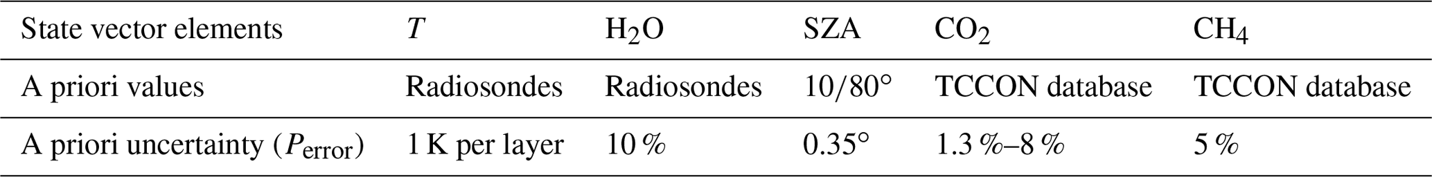
The IC analysis uses simulated radiance spectra of CHRIS in the bands TB, B1, B2 and B3. The CO2 and CH4 vertical concentrations of the a priori state vector xa are based on a profile that follows the criteria described in Sect. 3.1 and discretized by 40 vertical layers, extending from the ground to 40 km height with 1 km steps. In addition, the vertical water vapor profile, the temperature and the SZA are included in the nonretrieved parameters and are discussed in Sect. 3.3.3. The a priori values and their variabilities are summarized in Table 1 and are described in the following sections.
3.3.1 A priori error covariance matrix
In situ data and climatology can give us an evaluation of the a priori error covariance matrix Sa. Since the use of diagonal a priori covariance matrices is common for retrievals from space measurements (e.g., De Wachter et al., 2017), and since this study is dedicated to information coming from measurement rather than climatology or in situ observations, we assume firstly that Sa is a diagonal matrix with the ith diagonal element (Sa,ii) defined as
where σa,i stands for the standard deviation in the Gaussian statistics formalism. The subscript i represents the ith parameter of the state vector. The CO2 profile a priori error is estimated from Schmidt and Khedim (1991). The CH4 a priori error is fixed to perror=5 %, similar to the one used in Razavi et al. (2009) for the retrieval of the methane obtained from IASI and also to be consistent with the previous study concerning the TANSO-FTS instrument (Herbin et al., 2013a).
Nevertheless, the correlation of the vertical layers is more expressed by the off-diagonal matrix elements. This is the reason we also use an a priori covariance matrix similar to the one used in Eguchi et al. (2010), where the climatology derived from TCCON is used to construct this matrix. The study with these two covariance matrices is presented for CHRIS in the following sections.
3.3.2 Measurement error covariance matrix
The measurement error covariance matrix is computed knowing the instrument performance and accuracy. The latter is related to the radiometric noise expressed by the SNR already discussed in Sect. 2.3. This error covariance matrix is assumed to be diagonal, and the ith diagonal element can be computed as follows:
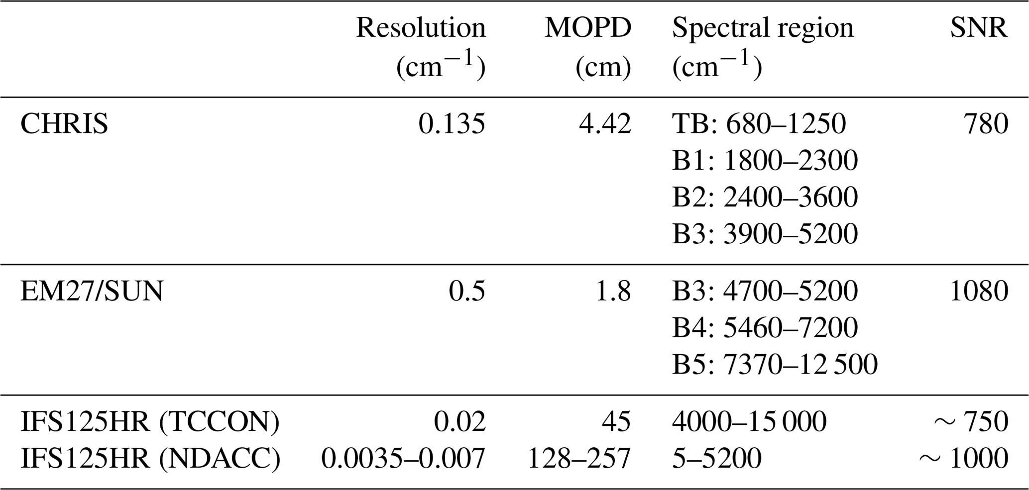
where σm,i is the standard deviation of the ith measurement (yi) of the measurement vector y, representing the noise-equivalent spectral radiance. The SNR for CHRIS is estimated to be 780, and it is reported with other instrumental characteristics in Table 3.
3.3.3 Nonretrieved parameter characterization and accuracy
The effects of nonretrieved parameters are a complicated part of an error description model. In our case these uncertainties are limited to the interfering water vapor molecules due to their important existence in the spectra and the effect of the temperature, where a vertically uniform uncertainty is assumed in both cases. It is important to note that in this study water vapor is considered as a nonretrieved parameter for the sake of comparison with Herbin et al. (2013a), but it will be part of the retrieved state vector in the inversion process, which will be the subject of a future study.
On the one hand, we assumed a partial column with an uncertainty (pCmol) of 10 % instead of a profile error for H2O. On the other hand, we assumed a realistic uncertainty of δT=1 K on each layer of the temperature profile, which is compatible with the typical values used for the European Centre for Medium-Range Weather Forecasts (ECMWF) assimilation. Moreover, we assumed a realistic uncertainty of 0.35∘ on the SZA, corresponding to the difference in the solar angle during the acquisition of a measurement corresponding to 100 scans. All these variabilities are reported in Table 1.
The total forward model error covariance matrix (Sf), assumed to be diagonal in the present study, is given by adding the contributions of each diagonal element, and the ith diagonal element (Sf,ii) is given by
Here, the spectroscopic effects such as the line parameter, the line mixing and the continua errors are not considered, but they are discussed with the XG column estimation in Sect. 3.4.2.
3.4 Information content analysis applied to greenhouse gas profiles
An information content analysis is performed on the whole spectrum for CO2 and CH4 separately to quantify the benefit of the multispectral synergy. Separately means that the state vector comprises only one of the above gas concentrations at each level between 0 and 40 km to match the altitudes reached by TCCON and the MAGIC instruments (balloons and planes reaching altitudes of more than 25 km). This corresponds to the case in which we estimated each gas profile alone when all other atmospheric parameters and all other gas profiles are known from ancillary data with a specific variability or uncertainty. Two different SZAs (10 and 80∘) are chosen to demonstrate the effect of the solar optical path on the study since the sensitivity is correlated to the viewing geometry. Furthermore two different a priori covariance matrices are used to show the effect of using climatological data describing the variability of GHG profiles. In the following subsections, we explain in detail the averaging kernel, error budget and total column estimations.
3.4.1 Averaging kernel and error budget estimation
Figure 8 shows the averaging kernel A and total posterior error Sx for CO2 for an angle of 10∘. The figures of the second SZA (80∘) are not shown since the vertical distribution of the kernels and errors is quite similar and exhibits only slight differences in the amplitude with respect to the other angle. However, the results are different; they are discussed in order to quantify the information variability with the viewing geometry. A is obtained for CO2 independently using the variability introduced in Sect. 3.3.1 and considering an observing system composed of the band BT, B1, B2 or B3 separately and all the bands together to quantify the contribution of each of the spectral bands and show the benefits of the TIR–SWIR spectral synergy. Each colored line represents the row of A at each vertical grid layer. Each peak of A represents the partial degree of freedom of the gas at each level that indicates the proportion of the information provided by the measurement. In fact, if the value is close to unity, it means that the information comes predominantly from the measurement, but a value close to zero means that the information comes mainly from our prior knowledge of the a priori state. We can clearly see that at lower altitudes and up to 10 km, the kernels are close to unity, suggesting that the measurement improved our knowledge, while at higher altitudes (beyond 10 km) the kernels are close to zero. It is also important to note that when using all the bands simultaneously, the information distribution of the kernels is improved and is more homogeneous along the vertical profile.
Table 2The total column errors for CO2 and CH4 profiles for CHRIS for the two SZAs. The uncertainties are shown in percentages (%).
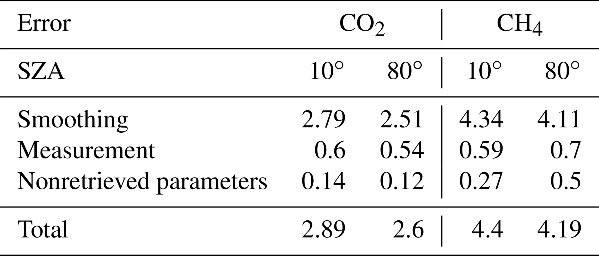

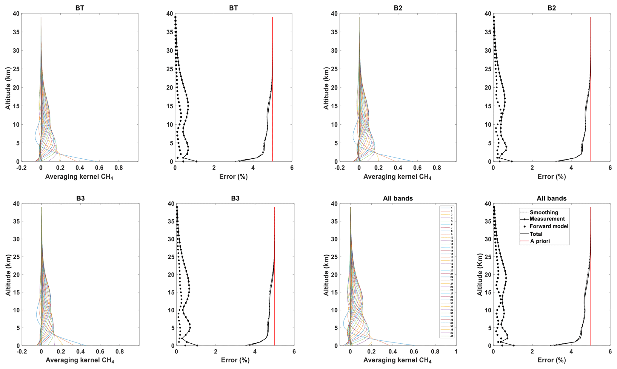
Figure 8Averaging kernels and error budgets of vertical CO2 profiles for bands TB, B1 and B3 separately and all the bands together for an angle of 10∘ for CHRIS. The red and solid black lines stand for the prior (Sa) and posterior (Sx) errors, respectively; the smoothing (Ssmoothing), measurement (Smeas.) and forward model parameter (Sfwd.mod.) errors are dash-dotted, dash-starred and dotted, respectively.
The measurement may provide information about CO2 from the ground up to 20 km high in the atmosphere (all bands), while at much higher altitudes the information comes mainly from the a priori profile due to a smaller sensitivity of these gases in the upper troposphere. This is clearly represented in the error budget study: the a posteriori total error (solid black line) is significantly smaller than the a priori error (red line) in the lower part of the atmosphere (between 0 and 20 km), which means that the measurement improved our knowledge of the CO2 profile. Beyond 20 km, the total a posteriori error is equal to the a priori error, suggesting a very poor sensitivity at high altitudes. Furthermore, one can notice that the measurement error stays very weak regardless of the band used, which proves that the error related to the SNR is negligible. Furthermore, the forward model error depending on the nonretrieved parameters remains quite modest. However, the smoothing error predominates over the other errors and becomes preponderant beyond 20 km, which means that the information is strongly constrained by the a priori profile at high altitudes, and little information is introduced from the measurement. To overcome this problem, another similar study was conducted but with a nondiagonal a priori covariance matrix (Eguchi et al., 2010). The vertical distribution is more homogeneous through all the layers. The shape of the error budget is very similar to that of the variance; however, the a priori and a posteriori errors are significantly reduced. The measurement and forward model errors remain weak, but it is important to note that despite the fact that the smoothing error is smaller, the constraint is stronger. This has the effect of decreasing the uncertainty but also increasing the propagation of the smoothing error along the vertical layers, which explains the smaller values of the DOFSs.
Finally, the total DOFSs for CO2 are shown in Table 4 for angles of 10 and 80∘. It shows that for a diagonal a priori covariance matrix, one might be able to retrieve between two and three partial tropospheric columns for CO2, and as expected the DOFS value is slightly higher at 80∘ since the optical path of the sun in every layer is longer. However, when using a nondiagonal a priori covariance matrix, one less partial tropospheric column is retrieved but with significant improvement in the error budget estimation.
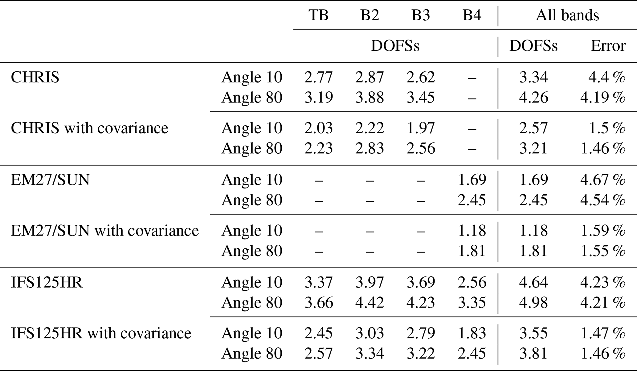
The same reasoning is followed for CH4: A is obtained for CH4 independently using the variability introduced in Sect. 3.3.1 and considering an observing system composed of the band TB, B1, B2 or B3 separately and all the bands together. Figure 9 shows that the vertical distribution of CH4 is more homogeneous than that of CO2, and we can see that the A's are broader than those of CO2, suggesting a very important correlation between layers. The use of all the bands simultaneously, just like CO2, improves the information distribution along the vertical profile. The forward model error is larger than that of CO2 since methane is more affected by the interfering species. The smoothing error is significantly larger than CO2 since it is constrained by a much higher a priori profile variability, which suggests a more direct effect on the retrieval of CH4. Similar to CO2, when using a nondiagonal a priori covariance matrix, the vertical distribution is very analogous to that of the variance only. However, the a priori and a posteriori errors are significantly reduced. The total DOFSs for CH4 are shown in Table 5 for both SZAs. This parameter shows that, for a diagonal a priori covariance matrix, three partial tropospheric columns and one additional partial column for an SZA of 80∘ can be retrieved. Finally, while using a nondiagonal a priori covariance matrix the DOFSs show that one less partial column is retrieved.
As a general result, the simultaneous use of all the bands instead of using each one separately increases the total DOFSs and systematically reduces the total errors of the two species. Moreover, using a climatological a priori covariance matrix shows the importance of reducing the error of the retrieved partial columns. Finally, the total profile error is derived from the relative values of the diagonal matrix of Sx (see Tables 4 and 5), which are discussed in detail in the following section.
Table 3Instrumental characteristics of CHRIS, the EM27/SUN and the IFS125HR of both NDACC and TCCON.
3.4.2 Total column estimation and uncertainty
Ground-based instruments like the one used in the TCCON network and the EM27/SUN operate in the NIR, where the column-averaged dry-air mole fractions (denoted XG for gas G) are calculated by monitoring the observed O2 columns. XG is calculated by rationing the gas-retrieved slant column to the O2-retrieved slant column for the same spectrum. Especially among the NDACC community, another method is used to calculate XG without using the oxygen reference. Based on the formula given in Wunch et al. (2011) and used in Zhou et al. (2019), we can calculate XG for CO2 and CH4:
where and are the mean molecular masses of water and dry air, respectively; Ps is the surface pressure; and gair is the column-averaged gravitational acceleration. Therefore, the calculation of XG is possible if all these parameters are available, particularly within the MAGIC framework, where we have access to the balloons and radiosondes data (temperature, surface pressure, relative humidity etc.) along with all the instruments involved. Thus, for these particular campaigns, XG values will be calculated for CHRIS using ARAHMIS, and the results will be compared with the other instruments involved, especially the IFS125HR of the TCCON network and the EM27/SUN. This will be the subject of an upcoming paper. However, the two equations for the calculation of XG are not strictly similar since the EM27/SUN eliminates the systematic errors that are common to the target gas and O2 column retrievals, which will not be possible for us since the O2 band is not detected by CHRIS.
In addition, the total column uncertainty is calculated by adding the concentration of each layer along the profile, weighted by the column of dry air based on Figs. 8 and 9. Table 2 lists the propagated uncertainties of the total column for both SZAs using a diagonal a priori covariance matrix: the uncertainty of the total CO2 column is 2.89 % and 2.6 % for 10 and 80∘, respectively, while the uncertainty for the total CH4 column is 4.4 % and 4.19 % for 10 and 80∘, respectively. The uncertainties are smaller for an SZA of 80∘ because the information distribution is improved with a longer OPD. Furthermore, these results show that the total profile error for CH4 is almost 2 times higher than that of CO2, but this is explained by the fact that our profile error is limited by the a priori profile error, which is much higher for CH4 than for CO2. The dominating component of the uncertainty comes from the smoothing, which predominates over the other uncertainties for both GHGs and is the major contributor to the total profile error. H2O, temperature and SZA are the most important parameters contributing to the forward model; they are represented by the nonretrieved parameter uncertainty. Additionally, it is important to note that there is a supplementary uncertainty associated with the spectroscopy unaccounted for in our study, which is purely systematic. It is not simple to evaluate in this case because we use different spectral domains, each having different spectroscopic uncertainties listed in the HITRAN database.
3.5 Comparison and complementary information content analysis for the IFS125HR, the EM27/SUN and CHRIS
During the MAGIC campaigns, several EM27/SUN and two IFS125HR instruments from the TCCON network were operated alongside CHRIS. An information content analysis is presented in the following sections for both of these instruments in order to compare and complement the study performed on CHRIS in Sect. 3.4.
3.5.1 Complementary information with the EM27/SUN
In this section, an IC study is performed for the EM27/SUN instrument in order to compare it with our results and to investigate the possibility of complementing the data we obtained from CHRIS, especially for MAGIC. The bands of the EM27/SUN used in this study are denoted as follows: B3 is the common band with CHRIS and has a spectral range of 4700–5200 cm−1, B4 goes from 5460 to 7200 cm−1, and B5 spans the spectral region between 7370 and 12 500 cm−1.
Firstly, a similar study to CHRIS is performed on the EM27/SUN for CO2 and CH4 separately. As mentioned in Sect. 3.4, the state vector comprises only one of the gas concentrations with the same profile at a layer going from 0 to 40 km; however, we took into account the SNR and spectral resolution specific to this instrument (see Table 3). Similar to the reasoning for CHRIS followed in Sect. 3.4, this study shows that using all the EM27/SUN bands together leads to an improvement of the a posteriori error profile of CO2 concentrations, especially in the lower part of the atmosphere. Table 4 shows the DOFSs for CO2 of the EM27/SUN: using a diagonal a priori covariance matrix for an angle of 10∘, the total DOFSs for bands B3 (common band with CHRIS) and B4 as well as all bands together are 2.95, 1.63 and 3.03, respectively. If only band B3 is taken into consideration, which is the common band between the two instruments, the DOFSs of CHRIS in this band are, as stated before, 2.62 and 3.34 for an angle of 10 and 80∘, respectively, compared to 2.95 and 3.17 for the EM27/SUN. Therefore, the same number of partial columns can be retrieved using CHRIS (see Sect. 3.4) for CO2 in this band. Furthermore, similar to CHRIS, the total error is reduced with a more propagated smoothing error on the profile and a reduction in the DOFSs when using a nondiagonal a priori covariance matrix (Eguchi et al., 2010). As for CH4 and referring to Table 3, band 3 in this instrument begins (4700 cm−1) where the CH4 band ends (4150–4700 cm−1) in the IFS125HR and CHRIS. This is important because TCCON networks begin their measurements at 4000 cm−1, which allowed for the comparison with band 3 of CHRIS (for both CO2 and CH4). However, the EM27/SUN instruments have no exploitable signal before 4700 cm−1 (Gisi et al., 2012); therefore the CH4 absorption lines do not show in the common band between CHRIS and the EM27/SUN, so the results are not discussed here.
Secondly, a simultaneous IC study was performed on all the channels of both CHRIS and the EM27/SUN in order to analyze the complementary aspect of these two instruments. The results of this study are shown in Fig. 10. The DOFSs obtained for CO2 are 3.67 and 3.93 for angles 10 and 80∘, respectively; for CH4 they are 3.99 and 4.43. This indicates a significant improvement of the retrieval when the spectral synergy between TIR, SWIR and NIR is used, but it is less than the one obtained from space (for example TANSO-FTS in Herbin et al., 2013a) since the measurement is obtained from the same optical path.
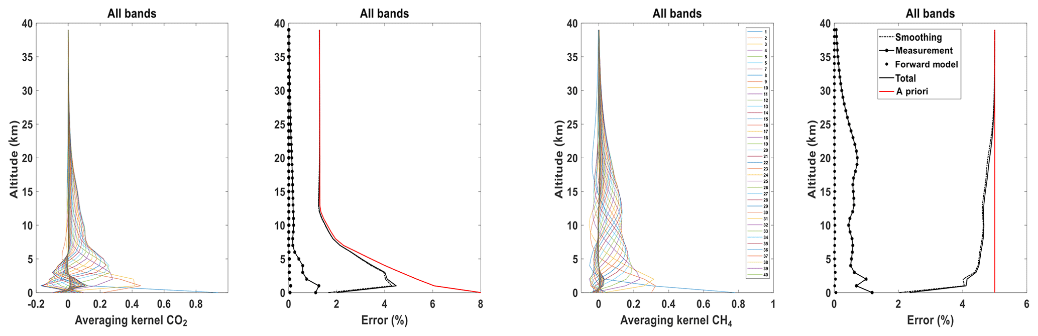
Figure 10Averaging kernels and error budgets of vertical CO2 and CH4 profiles for all the bands together for the EM27/SUN and CHRIS combined for an angle of 10∘. The red and black lines stand for the prior (Sa) and posterior (Sx) errors, respectively; the smoothing (Ssmoothing), measurement (Smeas.) and forward model parameter (Sfwd.mod.) errors are dash-dotted, dash-starred and dotted, respectively.
Table 4The DOFSs and column errors (%) of CO2 for each band and for each instrument.
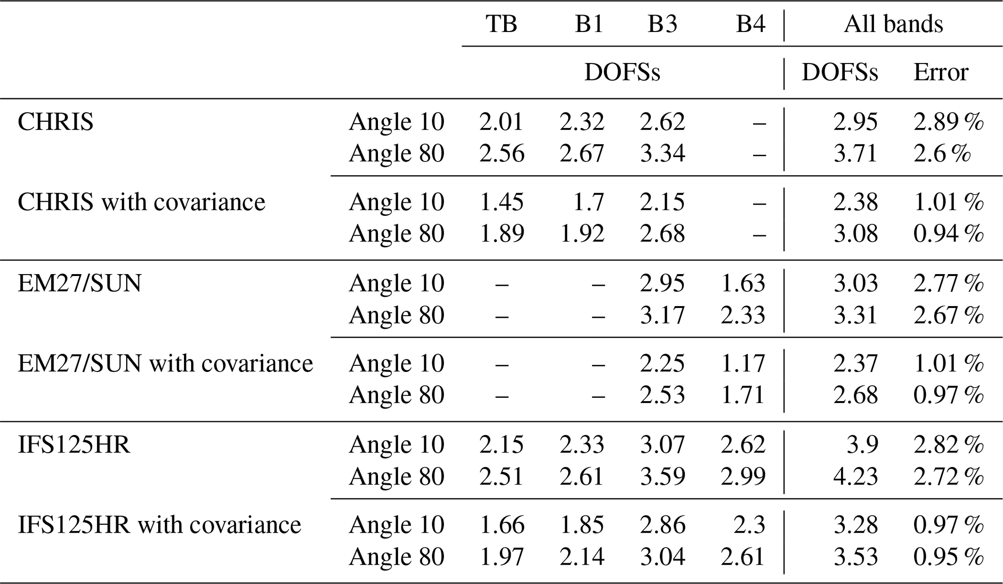
Table 5The DOFSs and column errors (%) of CH4 for each band and for each instrument.
3.5.2 Comparison with the IFS125HR
As mentioned before, the IFS125HR is a ground-based high-resolution infrared spectrometer used at NDACC and TCCON stations around the world. We performed a similar information content study only on the TCCON instrument since this network is involved in the MAGIC campaigns; therefore the results can be compared. For simplicity, the same annotation of the bands is kept for this section. The same methodology described in Sect. 3.4 is used here: the state vector comprises only CO2 and CH4 concentrations at a layer going from 0 to 40 km, where the SNR and the spectral resolution specific to the IFS125HR are taken into consideration (see Table 3).
We follow the same reasoning as in the sections before: Fig. 11 shows the averaging kernel A and the total posterior error Sx for CO2 and CH4 for an angle of 10∘. We can see that the vertical distribution is more homogeneous than CHRIS and the EM27/SUN, suggesting a high sensitivity at high altitudes, although in the lower atmosphere the a posteriori error Sx is significantly reduced. This is also shown in the error budget study: we can still distinguish the a posteriori total error (solid black line) from the a priori error (red line) even in the higher atmosphere. This is explained by the fact that the IFS125HR has a spectral resolution higher than both CHRIS and the EM27/SUN, so the measurement always improves our knowledge of the profile all along the atmospheric column. Furthermore, when using a nondiagonal a priori covariance matrix, the total profile error is significantly reduced, especially for CH4; however, the DOFSs are also reduced.
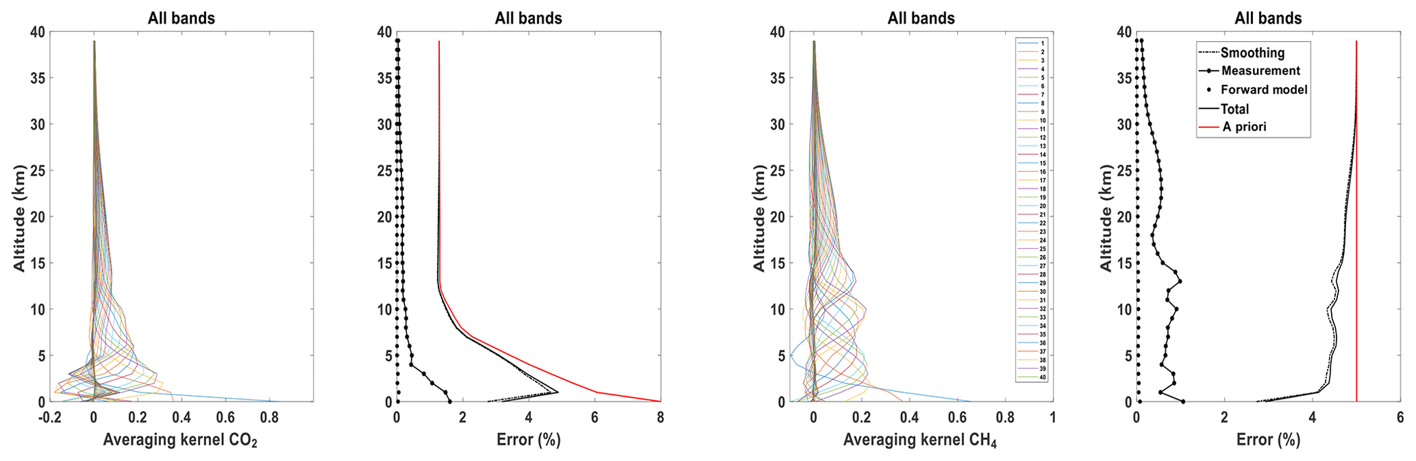
Figure 11Averaging kernels and error budgets of CO2 and CH4 and vertical profiles for all the bands together for an angle of 10∘ for the IFS125HR. The red and black lines stand for the prior (Sa) and posterior (Sx) errors, respectively; the smoothing (Ssmoothing), measurement (Smeas.) and forward model parameter (Sfwd.mod.) errors are dash-dotted, dash-starred and dotted, respectively.
Table 6Corresponding number of selected channels for the DOFSs of CO2 and CH4 and their respective percentage of the total number of channels for CHRIS.
The DOFSs of CO2 and CH4 are shown in Table 4 for both viewing angles and a priori covariance matrices. On the one hand, one additional partial tropospheric column for CO2 can be retrieved with respect to CHRIS for an angle of 10∘ and with respect to the EM27/SUN for both angles if all the bands are used. On the other hand, one additional partial tropospheric column can be retrieved for CH4 with respect to CHRIS for both angles if all the bands are used.

Figure 12Evolution of the DOFSs with the number of selected channels for CO2 (black) and CH4 (gray).
Using all the channels in the retrieval process has two disadvantages. First of all, it requires a very large computational time. Secondly, the correlation of the interfering species increases the systematic error. In this case, the a priori state vector xa and the error covariance matrix Sa are very difficult to evaluate. Channel selection is a method described by Rodgers (2000) to optimize a retrieval by objectively selecting the subset of channels that provides the greatest amount of information from high-resolution infrared sounders. L'Ecuyer et al. (2006) offer a description of this procedure based on the Shannon information content. Firstly, we create an “information spectrum” in order to evaluate the information content with respect to the a priori state vector. The channel with the largest amount of information is then selected. A new spectrum is then calculated with a new a posteriori covariance matrix that is adjusted according to the channel selected in the first iteration to account for the information it provides. In this way a second channel is chosen, based on this newly defined state space. This channel provides maximal information relative to the new a posteriori covariance matrix. This process is repeated, and channels are selected sequentially until the information in all the remaining channels falls below the level of measurement noise. As stated by the Shannon information content and noted in Rodgers (2000), it is convenient to work on a basis on which the measurement errors and prior variances are uncorrelated in order to compare the measurement error with the natural variability of the measurements across the full prior state. Therefore, it is desirable to transform the Jacobian matrix K (see Sect. 3.2) into using
which offers the added benefit of being the basis on which both the a priori and the measurement covariance matrices are unit matrices. Furthermore, Rodgers demonstrates that the number of singular values of greater than unity defines the number of independent measurements that exceed the measurement noise defining the effective rank of the problem.
Letting Si be the error covariance matrix for the state space after i channels have been selected, the information content of channel j of the remaining unselected channels is given by
where is the jth row of . Hj constitutes the information spectrum from which the first channel is selected. Taking the chosen channel to be channel l, the covariance matrix is then updated before the next iteration using the following statement:
In this way, channels are selected until 90 % of the total information spectrum H is reached in a way that the measurement noise is not exceeded.
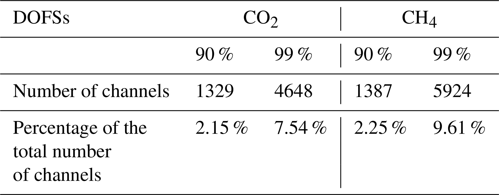
After that, H, expressed in bits, is converted to DOFSs to obtain Fig. 12, which represents the total DOFS evolution for CO2 and CH4 as a function of the number of selected channels for all spectral bands and for an SZA of 10∘. CHRIS has 75 424 channels in total; 13 800 are unusable because of the water vapor saturation between the bands, which leaves us with 61 624 exploitable channels. A preselection of these channels, based on Fig. 7, is done where the number of exploitable channels is reduced to the spectral areas where we find CO2 and CH4 (13 447 and 19 751 preselected channels, respectively). In Fig. 12, the DOFSs for each gas increase sharply with the first selected channels at first glance and then more steadily. The number of channels required to reach 90 % and 99 % of the total information is represented in Table 6. For CO2, out of the 1329 channels, 55.76 % of the information comes from B3 (common band with the EM27/SUN), 37.24 % from TB and 6.99 % from B1. As for CH4, out of the 1387 channels, 46.86 % of the information comes from B2, 28.19 % from TB and 24.9 % from B3. This result shows that most of the information for CO2 and CH4 comes from B3 and TB, respectively, which indicates that the synergy between TIR and SWIR observations is confirmed.
Furthermore, the 1329 and 1387 selected channels represent 2.15 % and 2.25 % of the 61 624 exploitable channels, respectively, so a retrieval process that uses selected channels corresponding to 90 % of the total information content would give comparable results to the one using the entire set of channels since almost 98 % of the information is redundant. Hence, these results indicate the interest of determining an optimal set of channels for each gas separately. This is why this channel selection will be used in the retrieval process, making it easier and less time consuming.
In conclusion, this paper presents the characteristics of the new infrared spectrometer CHRIS, which allows the retrieval of GHGs and trace gases. This instrumental prototype has unique characteristics such as its high spectral resolution (0.135 cm−1) and wide spectral range (680–5200 cm−1), covering the MIR region. In the context of its exploitation to retrieve GHGs, spectral and radiometric calibrations were performed using a calibrated external blackbody reaching a temperature of 1523 K. Additionally, between laboratory calibrations and during field campaigns the radiometric stability is monitored through measurements of the internal blackbody. Within the MAGIC framework, an extensive information content analysis is performed, showing the potential capabilities of this instrument to retrieve GHGs using two different SZAs (10 and 80∘) to quantify the improvement of the information with the solar optical path. Furthermore, two a priori covariance matrices were used: one diagonal and another derived from climatological data. The total column uncertainty is estimated, showing that when using a diagonal a priori covariance matrix the error for an angle of 10∘ is of the order of 2.89 % for CO2 and 4.4 % for CH4 for all the bands; however, when using a climatological distribution the total column error for the same angle and for all the bands is reduced to 1.01 % for CO2 and 1.5 % for CH4 but with a significant decrease in the DOFSs (from 2.95 to 2.38 for CO2 and from 3.34 to 2.57 for CH4). Furthermore, a comparison study with the IFS125HR of the TCCON, which is widely used in the satellite validation process, is performed, illustrating the benefits of its high spectral resolution for GHG retrievals. Moreover, a complementary study is carried out on the EM27/SUN to investigate the possibility of a retrieval exploiting the synergy between TIR, SWIR and NIR observations, which showed that a significant improvement can be obtained. For example, with an SZA of 10∘ the DOFSs are increased from 2.95 to 3.67. Finally, a channel selection is implemented to remove the redundant information. The latter will be used in future work dedicated to the CO2 and CH4 total column retrievals for the MAGIC campaigns.
All CHRIS data are available by contacting the authors.
MTEK and HH wrote the paper and produced the main analysis and results. FA, HH and MTEK designed the calibration study, performed the laboratory measurements and participated in the field campaigns. All authors read and provided comments on the paper.
The authors declare that they have no conflict of interest.
We acknowledge Fabrice Ducos for providing IT support and extensive expertise that greatly assisted this work and most of all for his great work on the ARAHMIS algorithm development. We would also like to thank the Ecole Centrale de Lille for its help on the radiometric calibration. Finally, we acknowledge Denis Petitprez from the PC2A laboratory for his experimental help on the ILS characterization.
This research has been supported by the CNES (Centre National d'Etudes Spatiales) TOSCA-MAGIC project.The CaPPA (Chemical and Physical Properties of the Atmosphere) project is funded by the French National Research Agency (ANR) through the PIA (Programme d'Investissement d'Avenir) (contract no. ANR-11-LABX-0005-01) and by the regional council Nord Pas de Calais-Picardie and the European Funds for Regional Economic Development (FEDER).
This paper was edited by Alyn Lambert and reviewed by two anonymous referees.
Aumann, H. H., Chahine, M. T., Gautier, C., Goldberg, M. D., Kalnay, E., McMillin L. M., Revercomb, H., Rosenkranz, P. W., Smith, W. L., Staelin, D. H., Strow, L. L., and Susskind, J.: AIRS/AMSU/HSB on the Aqua mission: design, science objectives, data products, and processing systems, IEEE T. Geosci. Remote, 41, 253–264, https://doi.org/10.1109/TGRS.2002.808356, 2003. a
Clarisse, L., Hurtmans, D., Prata, A. J., Karagulian, F., Clerbaux, C., Mazière, M. D., and Coheur, P.-F.: Retrieving radius, concentration, optical depth, and mass of different types of aerosols from high-resolution infrared nadir spectra, Appl. Optics, 49, 3713–3722, https://doi.org/10.1364/AO.49.003713, 2010. a
Clerbaux, C., Hadji-Lazaro, J., Turquety, S., George, M., Coheur, P.-F., Hurtmans, D., Wespes, C., Herbin, H., Blumstein, D., Tourniers, B., and Phulpin, T.: The IASI/MetOp1 Mission: First observations and highlights of its potential contribution to GMES2, Space Res. Today, 168, 19–24, https://doi.org/10.1016/S0045-8732(07)80046-5, 2007. a
Clough, S. A., Shephard, M. W., Mlawer, E. J., Delamere, J. S., Iacono, M. J., Cady-Pereira, K., Boukabara, S., and Brown, P. D.: Atmospheric radiative transfer modeling: a summary of the AER codes, J. Quant. Spectrosc. Ra., 91, 233–244, https://doi.org/10.1016/j.jqsrt.2004.05.058, 2005. a
De Wachter, E., Kumps, N., Vandaele, A. C., Langerock, B., and De Mazière, M.: Retrieval and validation of MetOp/IASI methane, Atmos. Meas. Tech., 10, 4623–4638, https://doi.org/10.5194/amt-10-4623-2017, 2017. a
Dohe, S., Sherlock, V., Hase, F., Gisi, M., Robinson, J., Sepúlveda, E., Schneider, M., and Blumenstock, T.: A method to correct sampling ghosts in historic near-infrared Fourier transform spectrometer (FTS) measurements, Atmos. Meas. Tech., 6, 1981–1992, https://doi.org/10.5194/amt-6-1981-2013, 2013. a
Eguchi, N., Saito, R., Saeki, T., Nakatsuka, Y., Belikov, D., and Maksyutov, S.: A priori covariance estimation for CO2 and CH4 retrievals, J. Geophys. Res., 115, D10215, https://doi.org/10.1029/2009JD013269, 2010. a, b, c
Gisi, M., Hase, F., Dohe, S., Blumenstock, T., Simon, A., and Keens, A.: XCO2-measurements with a tabletop FTS using solar absorption spectroscopy, Atmos. Meas. Tech., 5, 2969–2980, https://doi.org/10.5194/amt-5-2969-2012, 2012. a, b, c
Gordon, I. E., Rothman, L. S., Hill, C., Kochanov, R. V., Tan, Y., Bernath, P. F., Birk, M., Boudon, V., Campargue, A., Chance, K., Drouin, B. J., Flaud, J.-M., Gamache, R. R., Hodges, J. T., Jacquemart, D., Perevalov, V. I., Perrin, A., Shine, K. P., Smith, M.-A. H., Tennyson, J., Toon, G. C., Tran, H., Tyuterev, V. G., Barbe, A., Császár, A. G., Devi, V. M., Furtenbacher, T., Harrison, J. J., Hartmann, J.-M., Jolly, A., Johnson, T. J., Karman, T., Kleiner, I., Kyuberis, A. A., Loos, J., Lyulin, O. M., Massie, S. T., Mikhailenko, S. N., Moazzen-Ahmadi, N., Muller, H. S. P., Naumenko, O. V., Nikitin, A. V., Polyansky, O. L., Rey, M., Rotger, M., Sharpe, S. W., Sung, K., Starikova, E., Tashkun, S. A., Auwera, J. V., Wagner, G., Wilzewski, J., Wcislo, P., Yu, S., and Zak, E. J.: The HITRAN2016 molecular spectroscopic database, J. Quant. Spectrosc. Ra., 203, 3–69, https://doi.org/10.1016/j.jqsrt.2017.06.038, 2017. a, b
Herbin, H., Labonnote, L. C., and Dubuisson, P.: Multispectral information from TANSO-FTS instrument – Part 1: Application to greenhouse gases (CO2 and CH4) in clear sky conditions, Atmos. Meas. Tech., 6, 3301–3311, https://doi.org/10.5194/amt-6-3301-2013, 2013. a, b, c, d, e
Kobayashi, N., Inoue, G., Kawasaki, M., Yoshioka, H., Minomura, M., Murata, I., Nagahama, T., Matsumi, Y., Tanaka, T., Morino, I., and Ibuki, T.: Remotely operable compact instruments for measuring atmospheric CO2 and CH4 column densities at surface monitoring sites, Atmos. Meas. Tech., 3, 1103–1112, https://doi.org/10.5194/amt-3-1103-2010, 2010. a
L'Ecuyer, T. S., Gabriel, P., Leesman, K., Cooper, S. J., and Stephens, G. L.: Objective Assessment of the Information Content of Visible and Infrared Radiance Measurements for Cloud Microphysical Property Retrievals over the Global Oceans. Part I: Liquid Clouds, J. Appl. Meteorol. Clim., 45, 20–41, https://doi.org/10.1175/JAM2326.1, 2006. a
Michalsky, J. J.: The Astronomical Almanac's algorithm for approximate solar position (1950–2050), J. Sol. Energ., 40, 227–235, https://doi.org/10.1016/0038-092X(88)90045-X, 1988. a
Pathakoti, M., Gaddamidi, S., Gharai, B., Mullapudi Venkata Rama, S. S., Kumar Sundaran, R., and Wang, W.: Retrieval of CO2, CH4, CO and N2O using ground- based FTIR data and validation against satellite observations over the Shadnagar, India, Atmos. Meas. Tech. Discuss., https://doi.org/10.5194/amt-2019-7, 2019. a
Persky, M. J.: A review of spaceborne infrared Fourier transform spectrometers for remote sensing, Rev. Sci. Instrum., 66, 4763–4797, https://doi.org/10.1063/1.1146154, 1995. a
Petri, C., Warneke, T., Jones, N., Ridder, T., Messerschmidt, J., Weinzierl, T., Geibel, M., and Notholt, J.: Remote sensing of CO2 and CH4 using solar absorption spectrometry with a low resolution spectrometer, Atmos. Meas. Tech., 5, 1627–1635, https://doi.org/10.5194/amt-5-1627-2012, 2012. a
Razavi, A., Clerbaux, C., Wespes, C., Clarisse, L., Hurtmans, D., Payan, S., Camy-Peyret, C., and Coheur, P. F.: Characterization of methane retrievals from the IASI space-borne sounder, Atmos. Chem. Phys., 9, 7889–7899, https://doi.org/10.5194/acp-9-7889-2009, 2009. a
Revercomb, H. E., Buijs, H., Howell, H. B., LaPorte, D. D., Smith, W. L., and Sromovsky, L. A.: Radiometric calibration of IR Fourier transform spectrometers: solution to a problem with the High-Resolution Interferometer Sounder, Appl. Optics, 27, 3210–3218, https://doi.org/10.1364/AO.27.003210, 1988. a, b, c
Rodgers, C. D.: Inverse Methods for Atmospheric Sounding – Theory and Practice, Series on Atmospheric Oceanic and Planetary Physics, vol. 2, World Scientific Publishing Co. Pte. Ltd, Singapore, https://doi.org/10.1142/9789812813718, 2000. a, b, c, d
Schmidt, U. and Khedim, A.: In situ measurements of carbon dioxide in the winter Arctic vortex and at midlatitudes: an indicator of the age of stratopheric air, Geophys. Res. Lett., 18, 763–766, https://doi.org/10.1029/91GL00022, 1991. a
Schneider, M. and Hase, F.: Technical Note: Recipe for monitoring of total ozone with a precision of around 1 DU applying mid-infrared solar absorption spectra, Atmos. Chem. Phys., 8, 63–71, https://doi.org/10.5194/acp-8-63-2008, 2008.
Suto, H., Kuze, A., Kaneko, Y., and Hamazaki, T.: Characterization of TANSO-FTS on GOSAT, AGU Fall Meeting Abstracts, 2006. a
Toon, G. C.: Solar Line List for the TCCON 2014 Data Release, CaltechDATA, https://doi.org/10.14291/tccon.ggg2014.solar.r0/1221658, 2015. a, b
Trishchenko, A. P.: Solar Irradiance and Effective Brightness Temperature for SWIR Channels of AVHRR/NOAA and GOES Imagers, J. Atmos. Ocean. Tech., 23, 198–210, https://doi.org/10.1175/JTECH1850.1, 2006. a
Wiacek, A., Taylor, J. R., Strong, K., Saari, R., Kerzenmacher, T. E., Jones, N. B., and Griffith, D. W. T.: Ground-Based Solar Absorption FTIR Spectroscopy: Characterization of Retrievals and First Results from a Novel Optical Design Instrument at a New NDACC Complementary Station, J. Atmos. Ocean. Tech., 24, 432–448, https://doi.org/10.1175/JTECH1962.1, 2007. a
Wunch, D., Toon, G. C., Blavier, J.-F. L., Washenfelder, R. A., Notholt, J., Connor, B. J., Griffith, D. W. T., Sherlock, V., and Wennberg, P. O.: The Total Carbon Column Observing Network, Philos. T. R. Soc. A, 369, 2087–2112, https://doi.org/10.1098/rsta.2010.0240, 2011. a, b
Zhou, M., Langerock, B., Sha, M. K., Kumps, N., Hermans, C., Petri, C., Warneke, T., Chen, H., Metzger, J.-M., Kivi, R., Heikkinen, P., Ramonet, M., and De Mazière, M.: Retrieval of atmospheric CH4 vertical information from ground-based FTS near-infrared spectra, Atmos. Meas. Tech., 12, 6125–6141, https://doi.org/10.5194/amt-12-6125-2019, 2019. a