the Creative Commons Attribution 4.0 License.
the Creative Commons Attribution 4.0 License.
 | 17 Jul 2020
Application of low-cost fine particulate mass monitors to convert satellite aerosol optical depth to surface concentrations in North America and Africa
Daniel M. Westervelt
Aliaksei Hauryliuk
Albert A. Presto
Andrew Grieshop
Ashley Bittner
Matthias Beekmann
R. Subramanian
Low-cost particulate mass sensors provide opportunities to assess air quality at unprecedented spatial and temporal resolutions. Established traditional monitoring networks have limited spatial resolution and are simply absent in many major cities across sub-Saharan Africa (SSA). Satellites provide snapshots of regional air pollution but require ground-truthing. Low-cost monitors can supplement and extend data coverage from these sources worldwide, providing a better overall air quality picture. We investigate the utility of such a multi-source data integration approach using two case studies. First, in Pittsburgh, Pennsylvania, both traditional monitoring and dense low-cost sensor networks are compared with satellite aerosol optical depth (AOD) data from NASA's MODIS system, and a linear conversion factor is developed to convert AOD to surface fine particulate matter mass concentration (as PM2.5). With 10 or more ground monitors in Pittsburgh, there is a 2-fold reduction in surface PM2.5 estimation mean absolute error compared to using only a single ground monitor. Second, we assess the ability of combined regional-scale satellite retrievals and local-scale low-cost sensor measurements to improve surface PM2.5 estimation at several urban sites in SSA. In Rwanda, we find that combining local ground monitoring information with satellite data provides a 40 % improvement in surface PM2.5 estimation accuracy with respect to using low-cost ground monitoring data alone. A linear AOD-to-surface-PM2.5 conversion factor developed in Kigali, Rwanda, did not generalize well to other parts of SSA and varied seasonally for the same location, emphasizing the need for ongoing and localized ground-based monitoring, which can be facilitated by low-cost sensors. Overall, we find that combining ground-based low-cost sensor and satellite data, even without including additional meteorological or land use information, can improve and expand spatiotemporal air quality data coverage, especially in data-sparse regions.
- Article
(2798 KB) - Full-text XML
-
Supplement
(1458 KB) - BibTeX
- EndNote


Air quality is the single largest environmental risk factor for human health; outdoor air pollution exposure is estimated to have caused about 4 million premature deaths annually in recent years (WHO, 2016, 2018a). Particulate matter (PM), which represents a mixture of solid and liquid substances suspended in the air, is one of the most commonly tracked and regulated atmospheric pollutants globally (WHO, 2006). Exposure to fine PM is known to have major adverse health impacts (e.g., Schwartz et al., 1996; Pope et al., 2002; Brook et al., 2010). In addition, PM mass concentration is often used as a proxy for overall air quality (WHO, 2018a). PM mass concentration is typically tracked as PM10 (total PM mass with diameter below 10 µm) and/or PM2.5 (total PM mass with diameter below 2.5 µm). Even at low concentrations, PM can have significant health impacts (Bell et al., 2007; Apte et al., 2015). These health impacts are especially notable in low-income communities and countries where they can interact with other socioeconomic risk factors (Di et al., 2017; Ren et al., 2018).
Sub-Saharan Africa (SSA) in particular is affected by poor air quality, with less than 10 % of communities assessed by the WHO meeting recommended air quality guidelines compared with 18 % globally and 40 % to 80 % in Europe and North America (WHO, 2018b). This poor air quality manifests in terms of high infant mortality (Heft-Neal et al., 2018), increased risk of chronic respiratory and cardiovascular diseases (Matshidiso Moeti, 2018), and reduced gross domestic product (World Bank, 2016). Industrial development and climate trends will likely only exacerbate this problem in the future (Liousse et al., 2014; UNEP, 2016; Silva et al., 2017; Abel et al., 2018).
Many African countries have among the highest estimated annual average PM10 and PM2.5 concentrations, yet they are also among those with the lowest number of in situ regulatory-grade PM monitoring sites per capita. Figure 1 shows estimated average annual PM2.5 concentrations for various regions of the world versus the density of regulatory-grade monitoring sites in these regions (note that low-cost monitors are not considered) based on information from the Global Health Observatory (GHO). The GHO combines data from multiple sources, including data collected during different years and from sporadic field monitoring campaigns, and it is not necessarily reflective of continuous routine monitoring for all regions (WHO, 2017). This lack of continuous surface monitoring data makes it difficult to answer basic scientific and policy questions related to air quality assessment and mitigation (Petkova et al., 2013; Martin et al., 2019). A major reason for this gap is the high capital and operational costs of traditional ground-based air quality monitoring equipment. Two emerging technologies have the capacity to close this gap: satellite-based air quality monitoring and ground-based low-cost sensor systems.
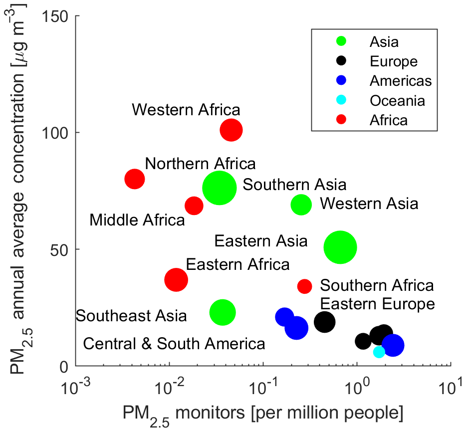
Figure 1Estimated annual average PM2.5 concentration versus the density of regulatory-grade monitoring stations across several global regions. Colors correspond to continents, and sizes roughly correspond to total regional population. This graphic is based on information available from the Global Health Observatory (WHO, 2017).
Satellites are much more expensive than traditional ground-based monitors, but their mobility and unique vantage point allow them to provide near-global coverage. Data from Earth-observing satellites can be used to assess air quality in a variety of ways. In particular, aerosol optical depth (AOD) retrievals quantify the absorption and scattering (extinction) of light by the atmosphere and can be related to the concentration of light-absorbing or light-scattering pollutants in the atmosphere. Several factors complicate the relationship between AOD and surface-level particulate matter mass concentrations (Paciorek and Liu, 2009). As a vertically integrated quantity, AOD is related to total light extinction by a column of atmosphere. The spatial distribution of particulate matter, especially vertical stratification, the presence or absence of plumes aloft, humidity, and the size and optical properties of particles affect the relationship between AOD and surface concentrations (Kaufman and Fraser, 1983; Liu et al., 2005; Paciorek et al., 2008; Superczynski et al., 2017; Zeng et al., 2018). Cloud cover also makes AOD retrievals impossible; the frequency of cloudy days in an area can therefore make it difficult to establish reliable relationships between AOD and surface PM, although this is not likely to be a concern for the continental US (Christopher and Gupta, 2010; Belle et al., 2017). Changes in surface brightness can also confound this relationship, although this may be less of an issue in developing countries with higher aerosol levels (Paciorek et al., 2012).
Nevertheless, early examinations of AOD data from the Moderate Resolution Imaging Spectroradiometer (MODIS) instrument, launched aboard the Terra and Aqua satellites in 1999 and 2002, showed good correlation (e.g., correlation coefficient r about 0.7 for Jefferson County, Alabama, in 2002) with surface PM2.5 concentrations in the United States, although these relationships varied from region to region (Wang and Christopher, 2003; Engel-Cox et al., 2004). For instance, correlations between AOD and hourly surface PM2.5 were found to vary from an r of 0.6 in the southeastern United States to an r of 0.2 in the southwestern United States during 2005–2006, with root mean square errors (RMSEs) of about 9 µg m−3 for surface PM2.5 reconstructed from AOD using linear relationships and with worse results over urban areas (Zhang et al., 2009). Additional studies show broadly similar relationships, with r ranging between about 0.5 and 0.8 in the northeastern United States (e.g., Paciorek and Liu, 2009), with changes in agreement depending on season (Chudnovsky et al., 2013a), and with better agreement at higher spatial AOD resolution (Chudnovsky et al., 2013b). Using additional covariates, such as land cover, land usage, and meteorological information, can further improve these relationships. In particular, surface PM2.5 estimation models combining daily averaged, 1 km resolution AOD data with meteorological and land use regression variables achieved an agreement (r) with EPA ground-based monitors of up to about 0.95 in the northeastern and 0.9 in the southeastern United States, with a mean absolute error of about 3 µg m−3 (Chang et al., 2014; Chudnovsky et al., 2014; Kloog et al., 2014). Methods incorporating the outputs of chemical transport models (in this case at lower spatial resolutions of 12 km compared to the 1 km AOD resolution and at daily temporal resolution) can further improve these results (e.g., Murray et al., 2019).
Models combining satellite AOD data with vertical profiles derived from chemical transport models tend to underestimate surface-level PM2.5 outside Europe and North America, mainly in India and China where ground-based comparison data are available (van Donkelaar et al., 2010, 2015). In China, the r between surface PM2.5 estimates derived from satellite AOD, meteorological, and land use information and measured surface PM2.5 was found to be about 0.8, corresponding to an RMSE of about 30 µg m−3 (roughly half the mean concentration) in resulting satellite-derived surface concentration estimates (Ma et al., 2014). A method that updates the relationships between AOD and surface PM2.5 on a daily basis (Lee et al., 2011) was able to improve these results, increasing r above 0.9 while reducing RMSE to about 20 µg m−3 (Han et al., 2018). This method, however, relies on local ground-based measurements to provide the data necessary to perform this daily updating.
Satellites have the potential to provide broad data coverage to previously unmonitored areas such as SSA. Satellite-based AOD and ground-based AOD agreed well during a recent assessment in West Africa (Ogunjobi and Awoleye, 2019), but an assessment in South Africa found a poor relationship between satellite AOD and surface PM2.5, with maxima in the surface concentrations coinciding with minima in the AOD (Hersey et al., 2015). Relationships between AOD and surface PM2.5 developed using ground monitoring data elsewhere in the world may not transfer well to SSA, leading to inaccurate quantification of surface air quality.
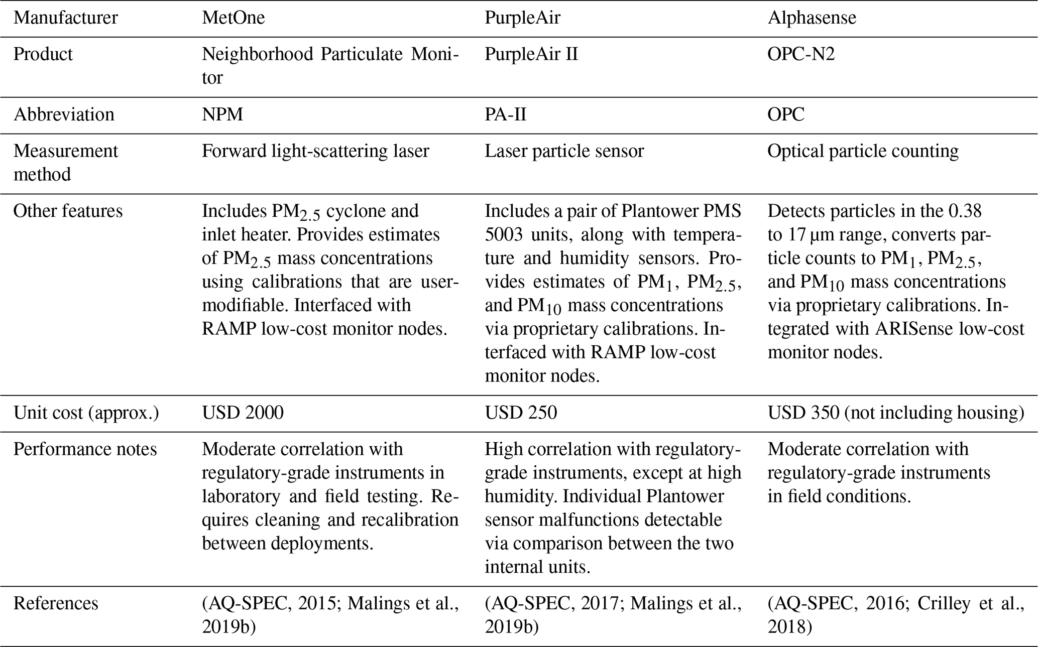
Low-cost air quality monitors have much lower purchase and operational costs in contrast to traditional or regulatory-grade monitors (Snyder et al., 2013; Mead et al., 2013). For example, a lower-cost multi-pollutant monitor (measuring gases and PM) costs a few thousand US dollars; single-pollutant PM sensors can cost just a few hundred US dollars. A comparable multi-pollutant suite of traditional air quality monitoring instruments would cost USD 100 000 or more; a regulatory-grade PM monitor can cost tens of thousands of US dollars (based on recent manufacturer quotations). This cost reduction is made possible by a combination of lower-cost measurement technologies (such as electrochemical sensors for gases and optical particle detectors for PM) and decreasing costs of battery, data storage, and communications technologies. Much recent research interest has been focused on assessing the performance of these technologies (e.g., AQ-SPEC, 2015, 2017), developing methods for accounting for cross-interference effects in gas sensors (e.g., Cross et al., 2017; Zikova et al., 2017; Kelly et al., 2017; Zimmerman et al., 2018; Crilley et al., 2018; Malings et al., 2019a) and humidity dependence in optical PM measurement methods (e.g., Malings et al., 2019b) to improve data quality, and demonstrating the utility of these low-cost monitors in various use cases (e.g., Subramanian et al., 2018; Tanzer et al., 2019; Bi et al., 2020). Because of their relatively low cost, these instruments can be deployed more widely than traditional monitoring technologies, enabling measurements in previously unmonitored areas. A trade-off for this increased affordability can be reduced accuracy compared to traditional air quality monitoring instruments. While there are currently no agreed-upon criteria for assessing low-cost monitor performance (Williams et al., 2019), several schemes suggest tiered rankings ranging from, for example, 20 % relative uncertainty for reasonable quantitative measurements to 100 % uncertainty for indicative measurements (Allen, 2018); this gives a general sense of the expected performance characteristics of such instruments. In particular, recent testing of two types of such low-cost monitors (which are the types used in this paper) found relative uncertainties on the order of 40 % and a correlation coefficient r of 0.7 with regulatory-grade instruments for hourly PM2.5 measurements (Malings et al., 2019b). These results are generally consistent with similar studies conducted in a variety of environments and concentration regimes, although relative performance tends to improve at higher concentrations (Kelly et al., 2017; Zheng et al., 2018).
Table 1Summary information for low-cost sensor systems utilized for this paper.
The potential exists to use both satellite and low-cost sensor data together to address the shortcomings of each data source individually and to fill existing data gaps globally. Satellite data provide near-global coverage, but relationships between AOD and surface PM2.5 do not generalize well across regions, so local ground-based data are needed for establishing conversion factors. Low-cost sensors can provide these local data in areas where existing monitoring networks are sparse or data are sporadically available. The current work examines the use of low-cost PM sensors as ground data sources for estimating surface concentrations from satellite AOD retrievals via two case studies. Specifically, we seek to quantify to what extent, even with the inherent uncertainties of low-cost sensors, their data might still be useful in estimating surface PM2.5 from AOD.
First, using a dense network of low-cost monitors in Pittsburgh, Pennsylvania, USA, where a regulatory-grade monitoring network already exists, we assess the utility of low-cost sensors compared to these traditional instruments. Second, using low-cost monitors deployed in Rwanda, Malawi, and the Democratic Republic of the Congo, we explore the utility of these low-cost sensors in previously unmonitored areas. We use US State Department data (publicly available from US government websites as well as the OpenAQ Platform at https://openaq.org, last access: 15 July 2020) from regulatory monitors at the US Embassies in Kampala (Uganda) and Addis Ababa (Ethiopia) to supplement our analysis of the relationship between converted satellite AOD data and surface-level PM2.5 across SSA. In this work, we focus on high-spatial- and temporal-resolution satellite data, which best align with the capacity of low-cost sensors to provide local air quality information in near-real time. We do not incorporate meteorological or land use information, as such additional information may not be available in sparsely monitored areas. Further, keeping the model as simple as possible avoids over-fitting a more sophisticated model to its calibration dataset, which can limit its generalizability. Instead, we use simple linear AOD-to-surface-PM2.5 conversion factors to indicate how low-cost sensors alone may provide additional information to inform the conversion of AOD to surface PM2.5, particularly in data-sparse domains. The techniques presented here are likely to translate to other data sources (e.g., new regulatory-grade monitors, new geostationary satellites) as they become available in the future.
2.1 Low-cost PM2.5 sensor data
Surface PM2.5 data were collected with three types of low-cost sensors (MetOne NPM, PurpleAir PA-II, and Alphasense OPC), as described in Table 1. For data collection, all NPM and most PA-II units were paired with RAMP lower-cost monitoring packages. The RAMP (Real-time Affordable Multi-Pollutant) monitor is produced by SENSIT Technologies (Valparaiso, IN; formerly Sensevere) and has internal gas, temperature, and humidity sensors, along with the capability to interface with external PM monitors (newer models also have internal PM sensors). This allows data collected by these PM monitors to be stored and transmitted over cellular networks by the RAMP. The characteristics and operation of the RAMP are described elsewhere (Zimmerman et al., 2018; Malings et al., 2019a). The ARISense node, manufactured by Quant-AQ (Somerville, MA; formerly manufactured by Aerodyne Research), is a lower-cost sensor package that combines internal gas, humidity, temperature, wind, and noise sensors, together with the Alphasense OPC-N2 PM sensor, and provides internet connectivity for data transmission (Cross et al., 2017). Most low-cost PM2.5 data are collected via one of these two systems; the exception is a single independently deployed PA-II unit in Kinshasa, DRC (see Table 2).
Collected data are down-averaged from their device-specific collection frequencies to a common hourly timescale. Erroneous data identified either automatically (e.g., negative concentration values or unrealistically high or low values) or manually (e.g., devices exhibiting abnormal performance characteristics identified during periodic inspections) are removed. To correct for particle hygroscopic growth effects (i.e., the impact of ambient humidity on the PM mass as measured by the low-cost sensors), previously developed calibration methods (Malings et al., 2019b) were implemented for the NPM and PA-II sensors. Briefly, a hygroscopic growth factor is first computed using the local humidity and temperature as measured by the low-cost monitor itself, along with an average or typical particle composition. Then, a linear correction is applied to the data based on past collocations with regulatory-grade monitoring instruments. Utilizing these methods, the uncertainties on hourly average PM2.5 concentration are about 4 µg m−3 (Malings et al., 2019b). For the Alphasense OPC sensors, raw bin-count numbers were integrated to produce a new concentration estimate for PM2.5, and a similar relative humidity correction was applied (Di Antonio et al., 2018). An additional correction factor of 1.69 (for workdays) or 1.39 (for non-workdays) was applied to data collected by NPM sensors in Rwanda based on previous results showing that current calibration methods tended to underestimate PM2.5 there (Subramanian et al., 2020). While we seek to use low-cost sensor data that have been calibrated and validated in accordance with best practices, uncertainties remain that are associated with these instruments and inaccuracies compared to regulatory-grade instruments. A major goal of this paper is to assess to what extent, even with these uncertainties, low-cost sensor data might still be useful in the context of the conversion of AOD to surface PM2.5.
Table 2Summary information for the ground sites presented in this paper.
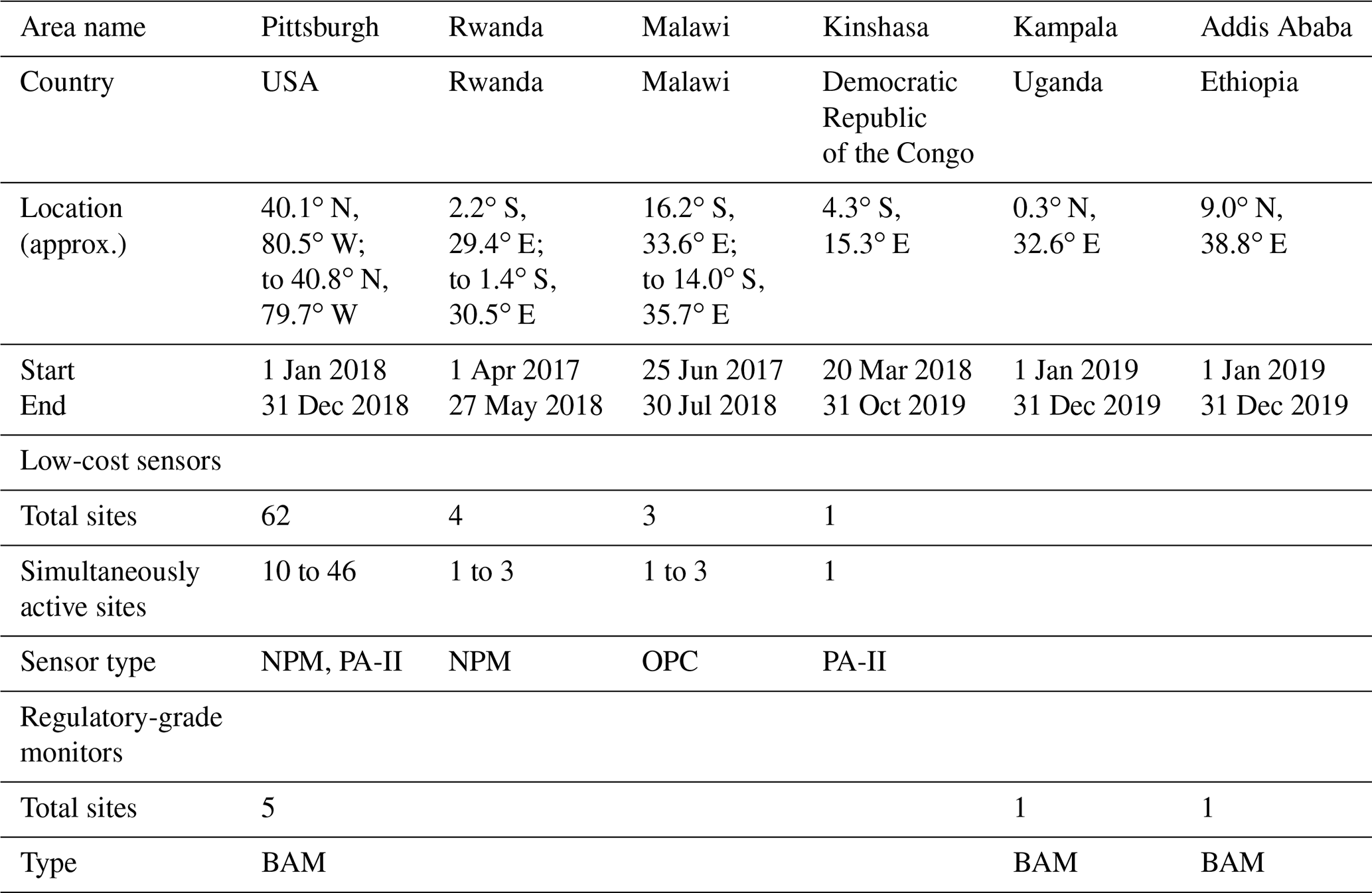

Figure 2Map of ground sites in the Pittsburgh area. Blue dots represent sites of regulatory-grade monitors used in the analysis, while red dots represent sites of low-cost sensor deployments. Background map obtained from http://maps.google.com (last access: 22 June 2020); map data ©2020 Google. Note the scale in the lower left corner. Also note that the pair of regulatory sites in the southeast of the map are located adjacent to a major industrial source (a coking plant for steel production), while the regulatory site to the northwest of the map is located adjacent to another industrial source (a chemical plant).
2.2 Ground-based sampling locations
Surface PM2.5 data analyzed in this paper were collected in seven different areas, as listed in Table 2, where the approximate locations, number of sites in each area, and durations of data collection are also listed. The Pittsburgh area includes sites in the surrounding Allegheny county, although most sites are concentrated within the city, as shown in Fig. 2. Similarly, the Rwanda area has most sites located in the capital city of Kigali, with one rural monitoring site collocated with the Mount Mugogo Climate Observatory in Musanze. In the Pittsburgh and Rwanda areas, low-cost sensors are connected with RAMP low-cost monitors. In Malawi, data are collected by three ARISense monitors using Alphasense OPC sensors deployed to three locations in the vicinities of Lilongwe and Mulanje. The two locations in the vicinity of Mulanje are village-center sites and so may be influenced by nearby combustion activities. In Kinshasa, a single PurpleAir PA-II was deployed independently (i.e., without an associated RAMP unit, as was the case in Pittsburgh) at the US Embassy. Temperature and humidity data were therefore obtained from the internal sensors within the devices themselves, and data connectivity was achieved using the local wireless internet network. At Kampala and Addis Ababa, regulatory-grade monitoring data collected at US Embassies are used to provide ground comparison data for concentration estimates derived from satellite AOD data. Additional information about all of these areas is also provided in the Supplement (Sect. S1), as are maps of the SSA sites (Figs. S4–S8).
2.3 Regulatory-grade instrument data
At several locations in the Pittsburgh area, as well as at the US Embassy locations in Kampala and Addis Ababa, hourly averaged ground-level PM2.5 data are also available from regulatory-grade monitoring instruments. In Pittsburgh, these monitors are operated by the Allegheny County Health Department (ACHD). At the US Embassies, these instruments are operated by the US State Department and the US EPA, and data are made available by these agencies (https://www.airnow.gov/international/us-embassies-and-consulates, last access: 15 July 2020), as well as by the OpenAQ Platform (http://openaq.org, last access: 15 July 2020). In all cases, regulatory-grade monitoring data are collected with beta attenuation monitors (BAMs), a federal equivalent monitoring method, that provide hourly PM2.5 concentration measurements for air quality index calculation purposes (Hacker, 2017; McDonnell, 2017). Nominally, such federal equivalent methods are required to be accurate within 10 % of federal reference methods (Watson et al., 1998; US EPA, 2016). Since BAM data have been used to establish the calibration methods for low-cost PM sensor data (Malings et al., 2019b), the data from the BAM instruments are used as provided for uniformity, without any additional corrections being applied.
2.4 Satellite data
The satellite data product used in this paper is the MODIS MCD19A2v006 dataset (Lyapustin and Wang, 2018) available through NASA's Earth Data Portal (http://earthdata.nasa.gov, last access: 15 July 2020). This dataset consists of AOD information for the 470 and 550 nm wavelengths from the MODIS system processed using the Multi-Angle Implementation of Atmospheric Correction (MAIAC) algorithm and presented at 1 km pixel resolution for every overpass of either the Aqua or Terra satellite (Lyapustin et al., 2011a, b, 2012, 2018). This represents a Level 2 data product, meaning that it includes geophysical variables derived from raw satellite data at each overpass time and has not been aggregated to a coarser (e.g., monthly) temporal resolution. Data from identified cloudy pixels are masked as part of the data product; possible misidentification of cloudy pixels is one source of error in relating surface PM2.5 and AOD. As per recommendations in the user guide for this dataset, only data matching “best quality” quality assurance criteria are used. This dataset was chosen as it represents the highest possible spatial and temporal resolution for AOD, thus providing the most points for comparison with the high-spatiotemporal-resolution low-cost monitor data.
Satellite AOD data are considered to be collocated in space with data from a ground site when the center of the AOD pixel is within 1 km of the ground site. Data are considered concurrent if the satellite overpass occurs within the hour interval over which ground site data have been averaged to arrive at the hourly average PM2.5 concentration value used. As we compare data from individual satellite passes directly to temporally collocated ground site data, we do not need to consider (as would be essential for long-term averages) the potential impact of the fraction of time during which satellite measures are missing (due to cloud cover or other factors). Likewise, we do not consider the biases associated with the fact that satellite passes occur at certain times of day (required when comparing with daily averaged ground monitoring data) since here we only compare AOD to surface PM2.5 during the same hour when the satellite pass occurs.
2.5 Conversion methods for satellite AOD
A linear regression approach is used to establish relationships between satellite AOD and surface-level PM2.5. Let yi,t denote the ground-level PM2.5 measurement at location i and time t, and let xi,t represent the satellite AOD (i.e., a vector combining the AOD at 470 or 550 nm wavelength with a “placeholder” constant of 1 to allow for the fitting of affine functions) corresponding to location i and time t. For this paper we present results using AOD at 550nm; results for AOD at 470 nm are similar and are included in the Supplement (Sect. S3.2). The total set of ground measurement sites in an area, S, is partitioned into two disjoint subsets. Subset Sin represents the sites used to establish the linear relationship between AOD and surface PM2.5 concentrations. The remainder of sites in the subset Sap are used for the application, i.e., to serve as an independent set to evaluate the performance of the linear relationship established from the Sin sites. Likewise, the time domain T is partitioned into initialization phase Tin, during which linear relationships are established, and application phase Tap, during which these relationships are applied and evaluated.
Linear relationships are determined as follows. First, satellite AOD data and surface PM2.5 monitor data from the Sin sites during the Tin phase are collected together:
A linear relationship is established between these, defined by parameters βin, using classical least-squares linear regression (e.g., Goldberger, 1980):
The covariance matrix of the parameters, , is also obtained:
where length(⋅) is a function returning the number of elements in the input. During the application phase, the linear relationship can be used to estimate the surface PM2.5 concentration at location i and time t, , from the satellite AOD data corresponding to that location and time:
The above procedure constitutes an offline or (in Bayesian terminology) prior conversion; i.e., it uses data collected during the initialization phase to define a single conversion factor that is applied throughout the application phase. An online, dynamic, or (in Bayesian terminology) posterior approach can also be adopted, in which this relationship is modified as additional data are available. This approach has been proposed by Lee et al. (2011) and evaluated by Han et al. (2018); it allows the potentially time-varying relationship between satellite AOD and surface PM2.5 concentration to be accounted for. In the online approach, for a time t during the application phase, a new dataset consisting of Yin,t and Xin,t is created by combining all data available from the Sin ground sites together with satellite AOD data for that time:
Based on these new data, a linear relationship is established for that time, as above:
This relationship is combined with the prior relationship established during the initialization phase (using a Bayesian approach and assuming normally distributed parameter values) to establish a new posterior relationship specific to that time, βt,post:
where diag(⋅) denotes a matrix diagonalization, and η is a relative error scale parameter used to define how much “weight” is given to the time-specific relationship parameters βt versus the prior relationship parameters βin in the updating process (with values of η near zero placing more weight on the time-specific relationships, while high values of η place more weight on the prior). The posterior relationship is then used to estimate surface PM2.5 concentrations from the satellite AOD data for that time:
Both the offline and online approaches are used in this paper, and their performance is compared (see Sect. 3.1).
This simple linear correction factor method does not explicitly account for vertical distribution profiles, cloud cover, or any other variables that affect the relationship of AOD to surface PM2.5. Instead, the aggregate effect of these variables is accounted for implicitly in an empirical relationship. The offline approach uses fixed relationships, which cannot account for time-varying effects such as changes in vertical distribution profiles. The online approach can account for these time-varying effects by assuming that their observed impact on the AOD-to-surface-PM2.5 relationship at the Sin sites is representative of their short-term impact throughout the region where the corresponding correction factors are applied. Finally, note that all parameters described above can be solved for analytically using the equations presented in this section (i.e., no iterative or approximate solution methods are necessary).
2.6 Analyses conducted in this paper
This section provides details on how the various analyses and comparisons to be discussed in Sect. 3 are performed. Additional details are also provided in the Supplement (Sect. S2.2 to S2.4).
2.6.1 Comparison of regulatory and low-cost monitors as ground stations to develop conversion factors for AOD
Here, we seek to compare the performance of AOD conversion to surface PM2.5 using either low-cost or regulatory-grade monitors as the ground-level data source for initialization. As only Pittsburgh has networks of both types of sensors in place, we focus our analysis in this area. The surface PM2.5 data collected at the five ACHD regulatory monitoring locations are used to assess the performance of the satellite AOD conversion, regardless of how the conversion factors are initialized. First, we use four of five ACHD locations to develop a conversion factor and apply it to the fifth. All ACHD sites are rotated through in this manner, providing a performance metric assessed for AOD conversion applied to each site. Second, we use low-cost sensors for developing the conversion factor; in this case, we select a subset of four locations in Pittsburgh where RAMP low-cost monitors are deployed so that the number of ground sites used matches the number of ACHD sites used in the first case. These low-cost monitor locations are chosen to provide a similar spatial coverage over Allegheny county as the ACHD sites. Low-cost monitors collocated with ACHD sites were specifically not chosen to allow for a fairer comparison when performance is assessed against these ACHD sites (since, if this were not done, it would be possible to have initialization sites that are collocated with the application sites, which was not possible when the ACHD sites alone were used). In this case, a conversion factor developed using the four low-cost sensor sites is applied at all five ACHD sites, with performance assessed at each site.
Different application cases of the satellite AOD conversion method are also tested. Note that in either case, we use all the collocated ground and satellite data across the entire time period without averaging these data in time. For a “yearly” conversion, data from the entire calendar year are used to develop the conversion factors, while in the “monthly” case, data from the previous month are used to develop conversion factors that are then assessed in the current month (e.g., January data are used to develop conversion factors that are applied in February, then the February data are used to develop conversion factors that are applied in March, etc.). For the monthly case, the median performance across months is presented. Although the yearly case would technically require having access to data that have not yet been collected (assuming this method is being applied for data collected in the current year), we use this to represent a case in which data from a previous year are used to develop conversions applied in the current year, as we assume that the annual average AOD-to-surface-PM2.5 concentration relationship for a given area will not significantly change from one year to the next. In addition, we also assess the relative performance of the offline (prior) conversion factors, for which the same relationship parameters determined during the initialization period are applied to the entire application period, and the online (posterior, dynamic) conversion, whereby these initial parameters are modified based on the AOD-to-surface-PM2.5 relationships specific to each individual satellite pass. The results of this analysis are discussed in Sect. 3.1.
2.6.2 Analysis of AOD conversion factor performance versus number of ground sites
A significant advantage of low-cost monitors compared to traditional instruments is that we can deploy tens to hundreds of low-cost sensors for the price of a single regulatory-grade monitor. To assess the potential benefits of this in terms of the conversion of satellite AOD data to surface PM2.5, we analyze the influence of the number of surface sites used on the performance of the surface PM2.5 estimates from AOD conversion. We again examine the Pittsburgh region, vary the number of ground sites used for initialization to generate the AOD conversion factor, and evaluate the performance using the ACHD regulatory monitoring network as the “ground truth”. For the ACHD network, the possible sites are the ACHD sites minus the one site against which performance is assessed (all ACHD sites are rotated through). For the low-cost sensors, the possible sites are all RAMP deployment locations in the area, excluding RAMPs that are collocated with ACHD sites, and performance is assessed against all ACHD sites. Subsets of varying size are randomly selected (10 different random set selections are used in this example); the mean of the performance metric across these 10 randomly selected sets is used as the assessed performance. In this case, a yearly online conversion factor is used (based on the performance of that method as described in Sect. 3.1). The results of this analysis are discussed in Sect. 3.2.
2.6.3 Comparison of converted AOD and nearest ground monitors as proxies for surface PM2.5
Here, we seek to assess the benefits of combining satellite AOD and ground-based sensor data compared to using ground-based sensor data alone. For this assessment, we compare estimates of surface PM2.5 derived from satellite AOD data using the methods presented previously in this paper with estimates based on the surface PM2.5 measurements alone, which we denote as “nearest monitor” estimates. For this estimation, we make use of a locally constant or naïve interpolation, in which the surface PM2.5 estimate for a given time and location is the same as the measurement of the nearest available ground monitor (i.e., one of the ground monitors used for establishing conversion factors for the satellite AOD data) at that time:
where dist(i,k) indicates the distance between locations i and k, and “argmin” denotes the input that minimizes this objective.
In this case, low-cost sensor data are used to represent the ground truth against which performance is assessed; this is done so that a comparable analysis can be made in Pittsburgh and Rwanda, since no regulatory-grade instruments were present in the latter area. Prior conversion factors are developed for the entire time period and are updated to posterior factors with time-specific data for their application. All but one low-cost sensor site in a given area are used for the development of these factors, with application and assessment on the final site. These sites are then cycled through to provide performance metrics across all sites. To allow for comparability between the nearest monitor approach and surface PM2.5 estimation from satellite AOD, we make use of the same set of ground sites for both; i.e., for each site, data from the closest available sites are used as inputs to the nearest monitor method, and all sites are cycled through in this manner, providing performance metrics for each site as above. The results of this analysis are discussed in Sect. 3.3 (for Pittsburgh) and 3.4 (for Rwanda).
2.6.4 Analysis of inter-seasonal generalization of AOD conversion factors
Changing seasons can affect the relationship between satellite AOD and surface PM2.5 due to changes in confounding factors like surface reflectance, aerosol vertical profiles, and particle composition. Here, we assess the utility of developing seasonal AOD conversion factors for Pittsburgh and Rwanda. For this assessment, conversions are developed and applied in specific seasons (information on these seasons is presented in Table S1 and Fig. S1). For Pittsburgh, these approximately correspond to winter, spring, summer, and fall, while in Rwanda, these represent alternating wet and dry seasons. For Pittsburgh, the major differences between seasons are related to temperature, with humidity varying to a lesser degree. In Rwanda, temperatures are relatively stable year-round, with seasons mainly differentiated by humidity changes (although the second dry season appears to have been unusually wet, comparable to the previous wet season).
RAMP data are used to represent ground truth concentrations for both areas. An offline or “prior” approach is used here in order to investigate the effect of generalizing a calibration developed in one season to a different season; i.e., calibrations are not modified based on data collected within the application period. Metrics are assessed for each individual site in each area, with all other sites being used to establish AOD conversion factors as in the previous section. The results of this analysis are discussed in Sect. 3.5.
2.6.5 Analysis of inter-regional generalization of AOD conversion factors
Finally, given the lack of ground-based monitoring in many parts of SSA, we assess whether a conversion factor developed in one city of this region can be generalized to other cities or locations across SSA. Here, a single AOD conversion factor is developed using one site in Kigali, Rwanda, and this factor is applied without modification to other sites across SSA. These include a second site in Kigali, a site in Musanze in rural Rwanda, a site in Kinshasa (DR Congo), and three sites in Malawi (one near the urban area of Lilongwe and two other sites in more rural areas to the south near Mulanje) where low-cost sensor systems are deployed. There are also two sites (Kampala, Uganda; Addis Ababa, Ethiopia) where hourly resolution long-term regulatory-grade monitoring data are available; data from these sites are included for comparative purposes. An offline approach is used here, with a single factor being initialized over the entire study period. Uncertainty estimates for the performance of this approach at each site are obtained via bootstrap resampling of the times with valid coincident satellite and ground data, with 100 random bootstrap samples being used to obtain the uncertainty estimates. The results of this analysis are discussed in Sect. 3.6.
In this section, we apply the proposed method for the satellite-AOD-to-surface-PM2.5 concentration conversion in several use cases. In Sect. 3.1, 3.2, and 3.3, we assess the performance in Pittsburgh by comparing the use of regulatory-grade monitors and low-cost monitors as ground sites for establishing conversion factors. In Sect. 3.4 and 3.5, we extend the comparison to Rwanda by examining the impact of using the relatively sparser low-cost sensor network there and examining seasonal variations in the conversions. Finally, in Sect. 3.6, we examine the generalization of Rwanda-based conversion factors to other locations across SSA. The assessment metrics used in this section, including correlation (r), the coefficient of variation of the mean absolute error (CvMAE), and the mean normalized bias (MNB), are described in the Supplement (Sect. S2.1).
3.1 Comparing the use of regulatory and low-cost monitors as ground stations to develop conversion factors for AOD
We first evaluate the utility of low-cost sensors as substitutes for regulatory-grade monitors when developing factors to convert satellite AOD data to surface PM2.5 estimates using the Pittsburgh area as our case study. Results for all eight combinations of ground initialization site monitor type (ACHD vs. RAMP), initialization period length (yearly vs. monthly), and application mode (prior vs. post.) are presented in Fig. 3. Overall, these results indicate relatively weak relationships between satellite AOD and surface PM2.5 for Pittsburgh, regardless of the method used. Correlations are weak (r < 0.5) and mean absolute errors are on the order of half to three-quarters of the concentration values (annual average concentrations are about 10 µg m−3 across most of Pittsburgh). Biases are low on average but can vary across locations. In comparing the different application modes, the posterior method provides better performance in terms of correlation than the prior method. This suggests that variability in AOD-to-surface-PM2.5 relationships between satellite passes (e.g., due to differences in the vertical profile of PM2.5 over the area and/or to differences between “point” measurements of the ground monitors and “area” AOD) is better captured by updating prior relationships with new information from each new satellite pass. In terms of other performance metrics, there is little difference between these application modes, with slight improvements observed in the posterior method for the RAMP data but slight decreases for the ACHD data. Comparing the use of annual to monthly initializations, performance metrics are slightly worse in the monthly case, indicating that the additional initialization data used in the yearly case generally lead to a more robust conversion. It should be noted, however, that these conclusions may be specific to relatively low PM2.5 concentrations as found in Pittsburgh.
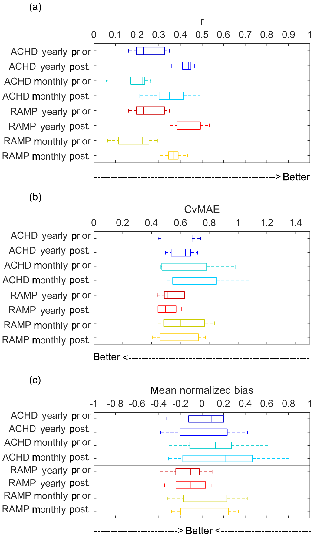
Figure 3Comparison of performance metrics (a correlation, b CvMAE, and c MNB) for surface PM2.5 estimated from satellite AOD data in the Pittsburgh area. Performance is assessed at the ACHD regulatory-grade monitoring sites. Ground sites used for factor development are either four of the ACHD monitors (ACHD) or four low-cost sensors associated with RAMP monitors (RAMP). Conversion factors are established either on a yearly or monthly basis. Finally, either an offline (prior) or online (post.) approach is used.
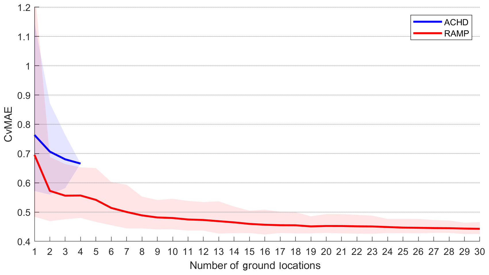
Figure 4Performance (assessed in terms of CvMAE) for surface PM2.5 estimated from satellite AOD data in the Pittsburgh area plotted as a function of the number of ground sites used. Performance is assessed against the ACHD regulatory-grade monitors. Solid lines indicate mean performance across sites using either ACHD or low-cost sensor (RAMP) sites to establish conversion factors. Shaded regions indicate the range of variability across application sites.
In all cases, performances using low-cost sensor data are comparable to those of the same conversion approaches utilizing the regulatory-grade instruments. Note that the low-cost monitors used here have been carefully corrected by collocation with regulatory-grade monitors (Malings et al., 2019b), which accounts for known artifacts with low-cost sensors. Thus, there is no evidence from this analysis of any inherent disadvantage to the use of carefully corrected low-cost sensors to provide ground data compared to more traditional instruments. Rather, based on these results, any additional uncertainty due to data quality differences between low-cost sensors and regulatory-grade instruments is seen to be negligible compared to the difficulties associated with relating satellite AOD to surface-level PM2.5 and has therefore had no systematic impact on the performance of the assessed linear conversion method, at least for this study area.
3.2 How many ground stations are needed to improve surface PM2.5 estimates from AOD retrievals?
Figure 4 shows the results of the assessment conducted as described in Sect. 2.6.2 in terms of the CvMAE metric. For small numbers of ground sites, results for the ACHD network and the low-cost sensor network are similar in terms of mean performance across different randomly selected subsets of the network, with slightly better performance using the RAMP network sites. This may be related to the smaller number of possible combinations of ACHD sites to be randomly selected compared to the RAMP sites; with more RAMP sites to choose from, the likelihood of selecting more generally representative (rather than more source-impacted) sites is higher, whereas with the ACHD network there is a high likelihood of choosing a heavily source-impacted site (especially since several ACHD locations are specifically chosen to monitor such local sources; see Fig. 2). The limited number of ACHD sites prevents this analysis from being expanded to larger numbers of locations; at four chosen locations, there is only one possible combination to be selected, so the spread in performance collapses to match the mean. With the low-cost sensor network, as more ground sites are included, mean CvMAE decreases until about 10 sites are chosen but afterwards remains relatively constant as more sites are included. Performance variability decreases as more site are added, indicating that by adding additional ground sites, even sites positioned at random throughout the domain, the conversion relationship becomes increasingly robust. While for a single ground monitor, worst-case CvMAE is on the order of 1.5 to 2, with 10 or more monitors, worst-case performance is improved below 0.6, which is a more than 2-fold improvement in worst-case performance. Overall, this demonstrates the potential benefits of dense low-cost sensor networks for the conversion of satellite AOD data, even over a limited spatial domain (covering about 600 km2). Furthermore, it shows that even with quasi-random placement of the ground sites, such as might be achieved by citizens making personal decisions to deploy low-cost monitors on their own properties, increasingly robust conversion results can be achieved as more sensors are included, although these benefits diminish beyond (at least in the case of Pittsburgh) about one monitor per 60 km2.
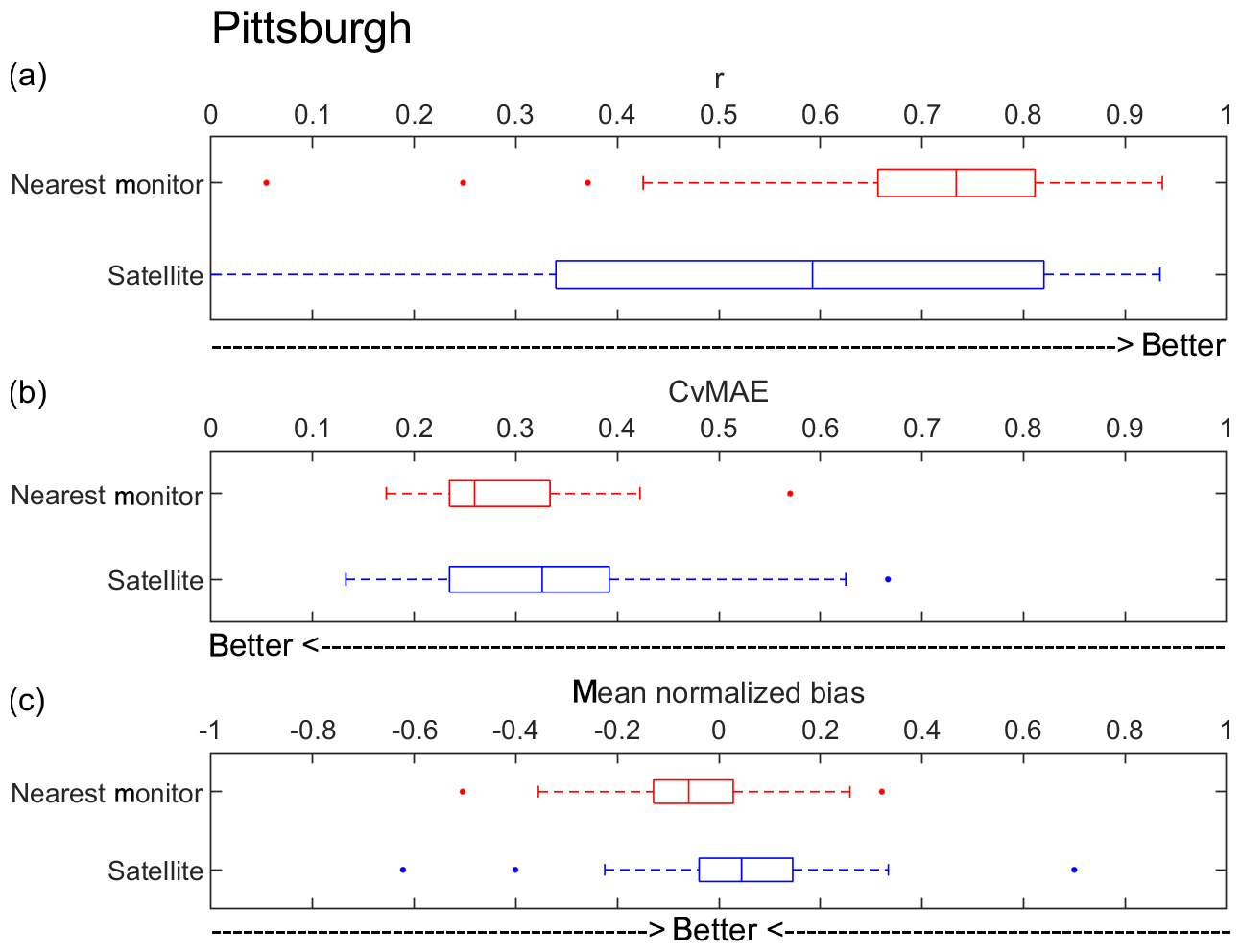
Figure 5Comparison of performance metrics (a correlation, b CvMAE, c MNB) for surface PM2.5 estimated either from satellite AOD data (satellite) or from the nearest ground-level PM2.5 monitor (nearest monitor) in the Pittsburgh area. Note that these performance metrics are not directly comparable to those presented in Fig. 3, as in this case a larger number of ground initialization sites (9 to 45, depending on the number of active sites in Pittsburgh at any particular time) are considered. Further, performance is now being assessed against the RAMP rather than the ACHD network (i.e., performance is assessed at the held-out active RAMP site); this is done to allow for comparability with the results from Rwanda presented in Fig. 6, where only RAMP data are available.
3.3 Comparison of AOD-based surface PM2.5 to measurements from a dense ground network
The performance of both the nearest monitor method and the satellite AOD conversion method is assessed for Pittsburgh in Fig. 5. It should be noted that all available ground sites have been used for conversion factor initialization in this section versus a limited subset of these in Sect. 3.1, leading to improved performance of this method following the trend noted in Sect. 3.2. In Pittsburgh, we see reduced performance (lower correlation, larger CvMAE) when using converted satellite data compared to nearest monitor data. This is likely a result of the quite dense network of low-cost sensors present in Pittsburgh, where the median distance between sensors in the network is about 1 km. With this dense network, there is a good chance that the nearest ground monitor will be quite close to the location at which concentrations are to be estimated, and the resulting nearest monitor estimate is therefore likely to be quite good, as PM concentrations tend to be homogenous at this spatial scale in Pittsburgh (Li et al., 2019). When PM2.5 is instead estimated from satellite data using a simple linear relationship, spatial and temporal variability in AOD-to-surface-PM2.5 relationships can confound the assessment. This is especially important considering the relatively low levels of surface PM2.5 concentration and AOD in and above Pittsburgh, meaning that any introduced noise will be relatively large in proportion to the signal being assessed. These results indicate that dense ground-based monitoring (if available) will likely outperform AOD-derived surface PM2.5, at least for the simple conversion method used here.
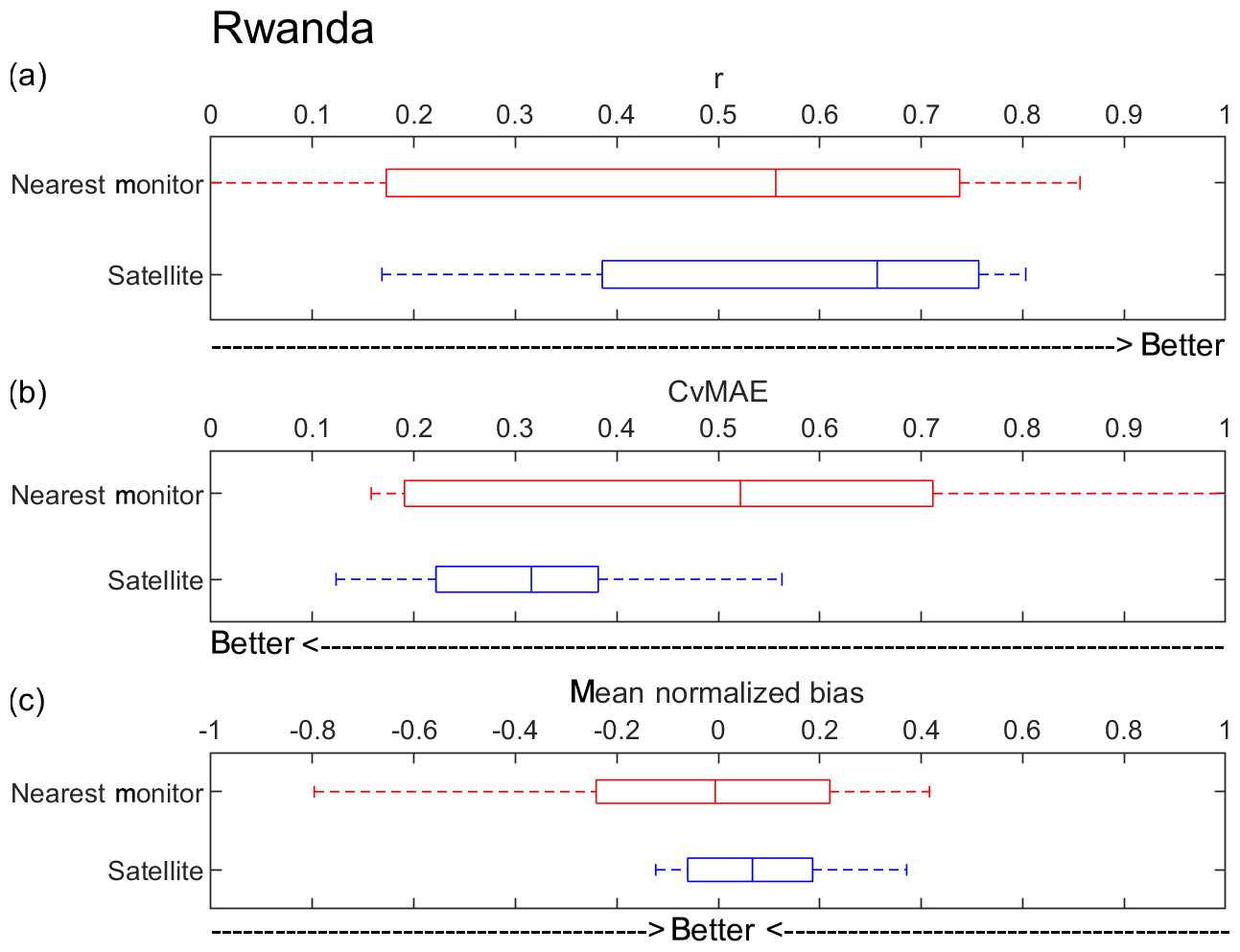
Figure 6Comparison of performance metrics (a correlation, b CvMAE, c MNB) for surface PM2.5 estimated either from satellite AOD data (satellite) or from the nearest ground-level PM2.5 monitor (nearest monitor) in the Rwanda area.
3.4 The utility of AOD-based surface PM2.5 in regions with a sparse ground monitoring network
The performance of the nearest monitor method and the satellite AOD conversion method is assessed for Rwanda in Fig. 6, in a similar manner as was done for Pittsburgh in Fig. 5. In Rwanda, we see an improvement across all metrics (higher and more consistent correlation, smaller and more consistent CvMAE, and less spread in the bias) as satellite data are combined with surface PM2.5 monitor data. Median CvMAE is reduced from about 0.5 to 0.3, which is a 40 % improvement. Because of the relative sparsity of the low-cost monitor network in Rwanda (four measurement sites, not all of which were simultaneously operational) compared to that in Pittsburgh, the assumption of the spatial homogeneity of concentrations between monitoring sites is less valid, so the inclusion of satellite data is beneficial in resolving these spatial differences. Furthermore, the relatively high levels of PM2.5 concentration in Rwanda (average of about 40 µg m−3 over the study period) allow for a higher signal-to-noise ratio relative to Pittsburgh. Together, these results indicate the high utility of low-cost sensors, used in conjunction with satellite data, when these are deployed even in relatively sparse networks to previously unmonitored areas with high surface PM2.5 concentrations.
This point is further explored in Fig. 7, which compares the correlations between ground measurements in Pittsburgh and Rwanda with the AOD-to-surface-PM2.5 correlations in these areas. In Pittsburgh, the high density of available monitors leads to relatively high inter-site correlations above the typical range of the AOD-to-surface-PM2.5 correlations. It is therefore difficult to extract meaningful patterns from the AOD information that would not also be present in available surface-level measurements, suggesting that AOD data provide little additional value in this densely monitored area (at least in terms of what can be derived without including additional information sources like atmospheric modeling and land use characteristics). Meanwhile, in sparsely monitored Rwanda, inter-site correlations are lower, overlapping the typical range of AOD-to-surface-PM2.5 correlations. This means that AOD data can still provide useful information for spatial heterogeneities in this region.
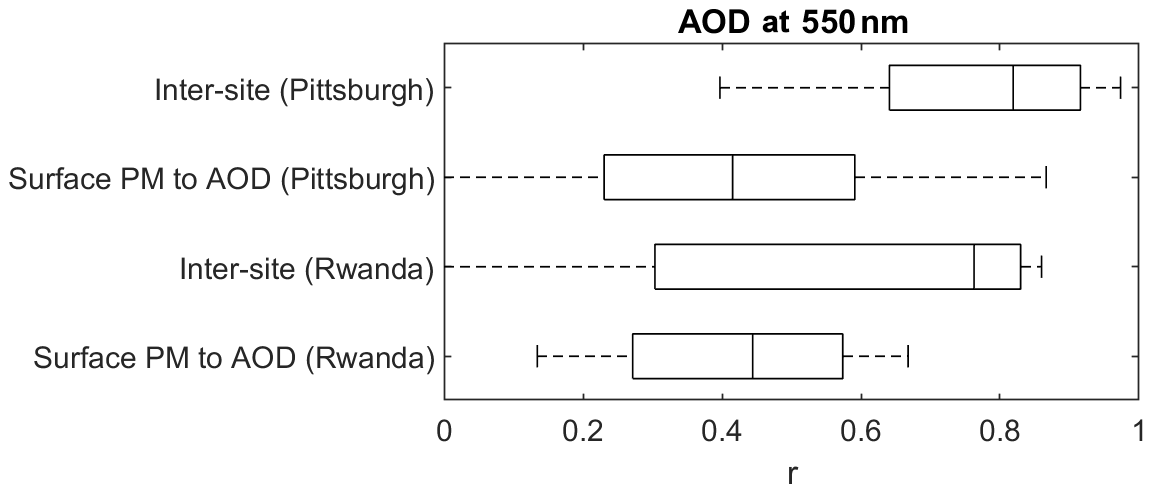
Figure 7Comparison of inter-site correlations versus AOD-to-surface-PM2.5 correlations in Pittsburgh and Rwanda.
3.5 Seasonal effects on satellite AOD conversion to surface PM2.5
Figure 8 presents the median performance metrics across all sites in either Pittsburgh or Rwanda for each combination of initialization and application season. Seasonal definitions are provided in Table S1. For Pittsburgh, spring conversion factors seem to generalize best when applied to other seasons, with the lowest biases and highest precisions. Low correlations are observed in the summer and winter regardless of initialization period, and clear seasonality is observed with summer initializations being biased high in winter and winter initializations being biased low in summer.
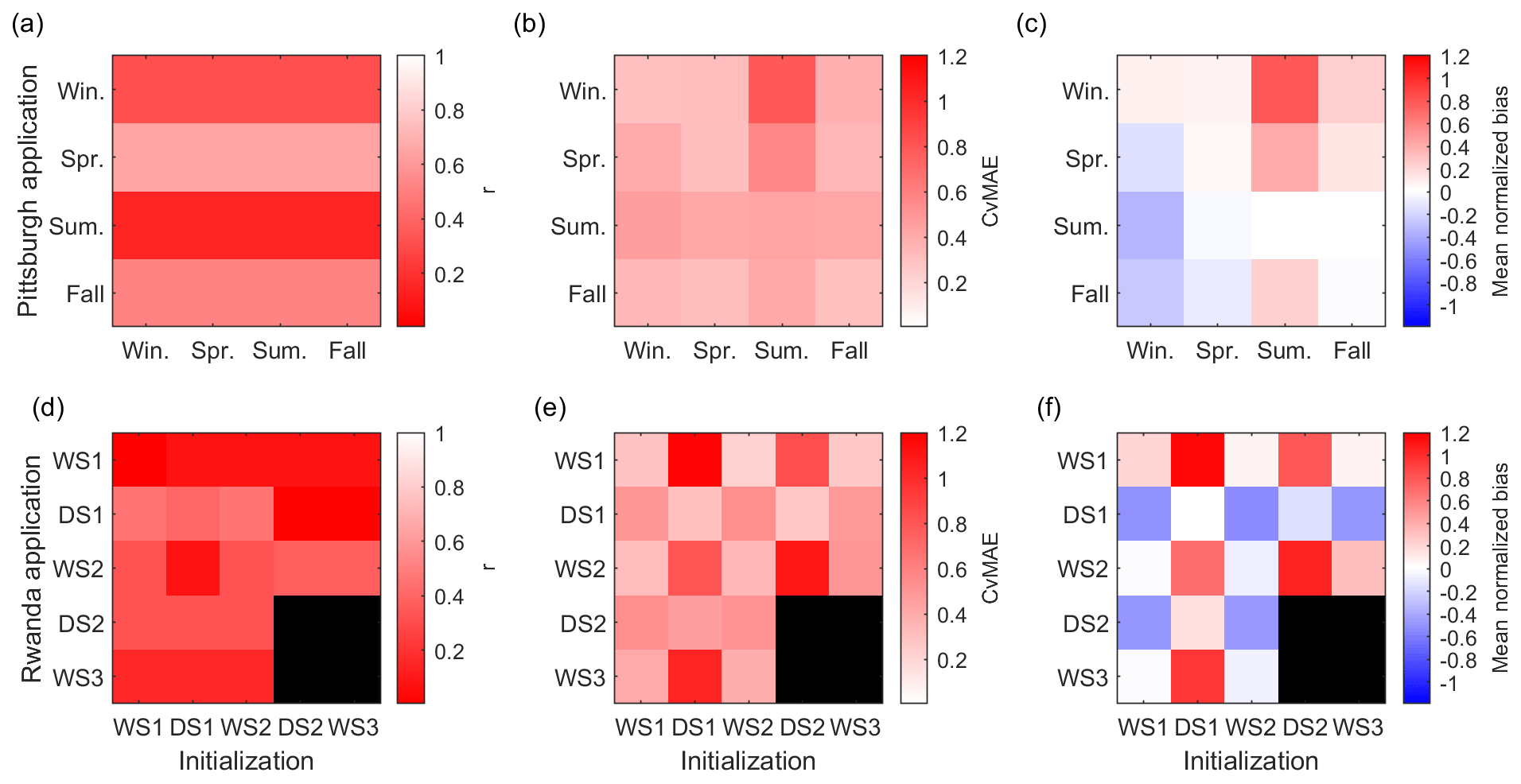
Figure 8Comparison of seasonal performance metrics (a, d correlation; b, e CvMAE; c, f MNB) for surface PM2.5 estimated from satellite AOD data across different seasons in the Pittsburgh (a, b, c) and Rwanda (d, e, f) areas. The horizontal axis differentiates the seasons during which initialization was performed, while the vertical axis denotes the seasons when the conversion was applied. Note that, in Rwanda, only one sensor was operational during Dry Season 2 (DS2) and Wet Season 3 (WS3), so the application of these conversions to an independent site was impossible; therefore, performance metrics are blacked out. In each figure diagonal (from top left to bottom right) elements correspond to the same season. Values are also listed in the Supplement (Table S8).
In Rwanda, an alternating pattern is revealed, with wet season conversion factors applying well to other wet seasons and dry season conversion factors applying to other dry seasons. Many factors could contribute to this pattern, including changes in humidity and the resulting impact on extinction, as well as seasonal burning patterns affecting particle sizes and compositions. Conversion factors appear to generalize better between wet seasons than between dry seasons. Correlations are highest during the first dry season (DS1), regardless of whether the conversion factor is developed during this season or during the surrounding wet seasons; this was also the driest season and the season with the highest PM2.5 concentrations. Applications of conversion factors developed in other seasons to DS1 underestimate PM2.5 in this season, especially applications of factors developed during the wet seasons (when PM2.5 levels were much lower). This indicates that there is seasonality to PM2.5 concentrations that is not being reflected in the AOD data and requires local monitoring to identify. Overall, these results indicate that conversion factors should be developed or updated at least on a seasonal basis, especially in Rwanda; a conversion factor developed during a limited monitoring campaign occurring in one specific season may fail to generalize well to other seasons.

Figure 9Comparison of performance metrics (a correlation, b CvMAE, c MNB) for surface PM2.5 estimated from satellite AOD data across multiple sites in SSA. The conversion factor is developed at a central site in Kigali, Rwanda; the distances of each testing site to this central site are given. Performances are assessed for all data collected at the given sites using the prior conversion factor only. Note that performance in Kampala and Addis Ababa is assessed using traditional reference monitors (indicated by *), while performance at the other sites reflects low-cost sensor data (indicated by •). Error bars denote the interquartile range of metric estimates obtained via bootstrap resampling (for most cases of the mean normalized bias, this range is smaller than the marker size).
3.6 Regional generalization of AOD conversion factors developed in Rwanda
Results of the analysis discussed in Sect. 2.6.5 are presented in Fig. 9. Correlation is relatively low across most application areas, with a weak trend of decreasing correlation as distance from the initialization site increases (the exception to this is found at the rural Mugogo site). The best performance in terms of CvMAE and normalized bias is found in Kigali, Kampala, and Kinshasa; these urban zones are likely most similar to the initialization site in terms of land use and resulting source mix. Relatively, the best performance is found at the spatially closest Kigali site. The Kampala site, with data collected via a traditional monitoring instrument, shows similar results as obtained at these other urban sites with low-cost monitors. The other more rural locations show poorer performance regardless of distance from the initialization site. However, the Addis Ababa site also shows much poorer performance despite also being an urban area, although the embassy is located on the outskirts of the city. This may be due to climate differences between Addis Ababa and the other cities considered, as well as differences in particle composition and size distributions, especially the higher contribution to AOD from coarse (larger than PM2.5) Saharan dust (De Longueville et al., 2010) that would not be accounted for in the Kigali-based AOD conversion factor.
These results indicate that, while conversion factors may generalize to sites with similar land use and climate characteristics, physical distance alone is not as significant in determining AOD–PM relationship generalizability. Also, the overall low correlation values indicate the importance of local data, as spatial heterogeneity in satellite-AOD-to-surface-PM2.5 relationships can be a concern even for nearby sites. Finally, it should be noted that a single annual conversion factor, as is assessed here, could fail to take into account seasonal variabilities (Sect. 3.5) and so can correlate poorly with surface PM2.5 even in or near the area where it is developed (as seen for the Kigali site here). A conversion factor that varies on at least a seasonal basis is therefore preferred; however, determining how to generalize such a time-varying conversion factor to other regions where seasonal definitions and characteristics can be quite different is a challenging problem. Overall, it does not appear from this analysis that AOD-to-surface-PM2.5 conversion factors can be broadly generalized across global regions with consistent results. Therefore, continuous localized monitoring, such as might be facilitated with local low-cost monitor networks, seems to be the most robust way to establish applicable AOD-to-surface-PM2.5 conversion factors.
We have examined the feasibility of using low-cost sensors as a data source in developing relationships between surface PM2.5 concentrations and satellite AOD. In a case study in Pittsburgh, there was no decrease in performance associated with the use of low-cost sensors for this purpose rather than more traditional regulatory-grade monitors, although performance was rather poor in both cases. The higher-density ground networks possible with low-cost sensors did provide benefits in terms of more robust conversion factors compared to the more sparsely deployed traditional monitoring network. However, it was found that for Pittsburgh, with a relatively dense low-cost sensor network (median inter-site distance of about 1 km) and low PM2.5 concentrations, the use of the nearest ground measurement sites outperformed the use of satellite AOD data to estimate surface PM2.5 using linear conversions. Partly, this could be because AOD is rather low over this area (average of about 0.2), leading to lower signal-to-noise ratios that reduce AOD-to-surface-PM2.5 correlation. Conversely, in Rwanda, a relatively sparse low-cost sensor network combined with satellite data in an environment with higher and more variable PM2.5 concentrations provided better estimates of surface PM2.5 concentrations than was available using only the nearest surface monitor alone. This result is highly relevant to SSA, as sparse local monitoring and high average PM2.5 concentrations (as measured by the few available ground-based monitors) are common features. Differences in seasonal characteristics (especially at the Rwanda locations) show the added value of season-specific conversion factors (which are facilitated by continuous local monitoring), while differences in characteristics between areas, especially urban and rural locations with highly variable particle types, limit the generalizability of conversion factors across regions (again emphasizing the importance of local monitoring).
The results presented here continue to highlight the need for ground-based PM2.5 monitoring in previously unmonitored areas such as SSA, especially in light of the benefits observed in Rwanda from having even a sparse ground monitoring network combined with satellite data for local spatial heterogeneity. Efforts to expand ground-based monitoring should make use of traditional regulatory-grade instruments wherever possible, supplemented with low-cost monitors to increase network density and expand spatial coverage. Findings in Pittsburgh indicate that denser monitoring networks, such as those made possible by low-cost sensors, improve the accuracy and robustness of surface PM2.5 estimates from satellites. Verification that the same trend will hold in other regions, especially in SSA, requires further dense deployments of low-cost sensors and is the subject of ongoing work.
It should be noted that the results of this paper pertain to local and instantaneous relationships using the highest spatial and temporal resolution of satellite data currently available. Results may differ for spatially or temporally aggregated satellite and ground site data. In fact, such spatial and temporal aggregation is likely to reduce the impact of noise (but not bias) both from low-cost instruments and from satellite retrievals. However, such aggregate information does not take full advantage of the potential inherent in low-cost sensors to provide near-real-time information on local air pollution. On a related point, satellite data (at least, for most of the world using current polar-orbiting platforms) cannot provide diurnal concentration profiles, instead presenting a “snapshot” of concentrations for a wide spatial domain but only for a specific time of day. Ground-based continuous monitoring, even with low-cost sensors, will still be essential where there is no coverage with geostationary platforms that provide continuous (for daytime only) retrievals (Judd et al., 2018; She et al., 2020). Past work has made use of AOD retrievals from GOES geostationary satellites for North America (Zhang et al., 2011, 2013). New geostationary satellites are planned for coverage of North America (the TEMPO satellite mission), Europe (Sentinel 4), and East Asia (GEMS); unfortunately, there are no current plans for coverage of Africa by similar satellites.
Further technical and research developments in this area have enormous promise for improving our understanding of local air quality worldwide. A functioning system for converting satellite to ground-level air pollution data, relying on a group of “trusted” ground data sources, could potentially be a valuable resource for assessing and correcting low-cost sensor data, allowing for in-field recalibration of drifting instruments and better identification of malfunctioning sensors. Low-cost systems combining PM mass measurement and ground-up AOD data can help to establish AOD-to-surface-PM2.5 relationships at finer spatiotemporal resolution (Ford et al., 2019). Open questions related to this research area include finding appropriate timescales over which conversion factors can be considered constant within regions as well as continuing to examine the question of conversion factor generalizability between regions separated by spatial distances and across different climates and land use characteristics. More sophisticated conversion methods incorporating meteorological and land use information as well as outputs of chemical transport models can also be considered, albeit with the recognition that some of these inputs may not yet be readily available or well validated for SSA.
Data related to the results and figures presented in this paper are available online at https://doi.org/10.5281/zenodo.3897454 (Malings et al., 2020). Codes related to the analysis of data and generation of figures are also provided at the same site.
The supplement related to this article is available online at: https://doi.org/10.5194/amt-13-3873-2020-supplement.
RS and MB were responsible for conceptualization. RS, AAP, and MB were responsible for funding acquisition. CM, DMW, AG, and AB developed the methodology. DMW, AG, and AB provided resources. CM and AH developed software. RS, AAP, and MB provided supervision. CM wrote the original draft. CM, DMW, AAP, AG, AB, MB, and RS participated in review and editing.
The authors declare that they have no conflict of interest.
This work benefited from state assistance managed by the National Research Agency within the “Programme d'Investissements d'Avenir” under reference ANR-18-MPGA-0011 (the “Make our planet great again” initiative). Measurements in Pittsburgh were funded by the Environmental Protection Agency (assistance agreement nos. RD83587301 and 83628601) and the Heinz Endowment Fund (grants E2375 and E3145). Measurements in Rwanda were supported by the College of Engineering, the Department of Engineering and Public Policy, and the Department of Mechanical Engineering at Carnegie Mellon University via discretionary funding support for Paulina Jaramillo and Allen Robinson. Andrew Grieshop and Ashley Bittner acknowledge support from NSF award CNH 1923568 to establish measurement sites in Malawi. The authors would like to thank Jimmy Gasore, Valérien Baharane, Abdou Safari Kagabo, Eric Lipsky, Sriniwasa P. N. Kumar, Provat Saha, Yuge Shi, Naomi Zimmerman, Rebecca Tanzer, and Rose Eilenberg for assistance with instrument setup and operation. Finally, the authors would like to thank Juan Cuesta and Jiayu Li for discussions and advice related to satellite data usage.
This research has been supported by the Agence Nationale de la Recherche (grant no. ANR-18-MPGA-0011), the U.S. Environmental Protection Agency (grant nos. RD83587301, 83628601), the Heinz Endowment Fund (grant nos. E2375, E3145), and the National Science Foundation (grant no. CNH 1923568). Discretionary funding support was provided by the College of Engineering, the Department of Engineering and Public Policy, and the Department of Mechanical Engineering at Carnegie Mellon University.
This paper was edited by Andrew Sayer and reviewed by two anonymous referees.
Abel, D. W., Holloway, T., Harkey, M., Meier, P., Ahl, D., Limaye, V. S., and Patz, J. A.: Air-quality-related health impacts from climate change and from adaptation of cooling demand for buildings in the eastern United States: An interdisciplinary modeling study, edited by: Thomson, M., PLOS Medicine, 15, e1002599, https://doi.org/10.1371/journal.pmed.1002599, 2018.
Allen, G.: “Is it good enough?” The Role of PM and Ozone Sensor Testing/Certification Programs, available at: https://www.epa.gov/sites/production/files/2020-02/documents/session_07_b_allen.pdf (last access: 15 July 2020), 2018.
Apte, J. S., Marshall, J. D., Cohen, A. J., and Brauer, M.: Addressing Global Mortality from Ambient PM2.5, Environ. Sci. Technol., 49, 8057–8066, https://doi.org/10.1021/acs.est.5b01236, 2015.
AQ-SPEC: Met One Neighborhood Monitor Evaluation Report, South Coast Air Quality Management District, available at: http://www.aqmd.gov/aq-spec/product/met-one---neighborhood-monitor (last access: 28 June 2018), 2015.
AQ-SPEC: Alphasense OPC-N2 Sensor Evaluation Report, South Coast Air Quality Management District, available at: http://www.aqmd.gov/docs/default-source/aq-spec/field-evaluations/alphasense-opc-n2---field-evaluation.pdf?sfvrsn=0 (last access: 5 December 2019), 2016.
AQ-SPEC: PurpleAir PA-II Sensor Evaluation Report, South Coast Air Quality Management District, available at: http://www.aqmd.gov/aq-spec/product/purpleair-pa-ii (last access: 28 June 2018), 2017.
Bell, M. L., Ebisu, K., and Belanger, K.: Ambient Air Pollution and Low Birth Weight in Connecticut and Massachusetts, Environ. Health Persp., 115, 1118–1124, https://doi.org/10.1289/ehp.9759, 2007.
Belle, J. H., Chang, H. H., Wang, Y., Hu, X., Lyapustin, A., and Liu, Y.: The Potential Impact of Satellite-Retrieved Cloud Parameters on Ground-Level PM2.5 Mass and Composition, Int. J. Env. Res. Pub. He., 14, 1244, https://doi.org/10.3390/ijerph14101244, 2017.
Bi, J., Stowell, J., Seto, E. Y. W., English, P. B., Al-Hamdan, M. Z., Kinney, P. L., Freedman, F. R., and Liu, Y.: Contribution of low-cost sensor measurements to the prediction of PM2.5 levels: A case study in Imperial County, California, USA, Environ. Res., 180, 108810, https://doi.org/10.1016/j.envres.2019.108810, 2020.
Brook, R. D., Rajagopalan, S., Pope, C. A., Brook, J. R., Bhatnagar, A., Diez-Roux, A. V., Holguin, F., Hong, Y., Luepker, R. V., Mittleman, M. A., Peters, A., Siscovick, D., Smith, S. C., Whitsel, L., Kaufman, J. D., and on behalf of the American Heart Association Council on Epidemiology and Prevention, Council on the Kidney in Cardiovascular Disease, and Council on Nutrition, Physical Activity and Metabolism: Particulate Matter Air Pollution and Cardiovascular Disease: An Update to the Scientific Statement From the American Heart Association, Circulation, 121, 2331–2378, https://doi.org/10.1161/CIR.0b013e3181dbece1, 2010.
Chang, H. H., Hu, X., and Liu, Y.: Calibrating MODIS aerosol optical depth for predicting daily PM2.5 concentrations via statistical downscaling, J. Expo. Sci. Env. Epid., 24, 398–404, https://doi.org/10.1038/jes.2013.90, 2014.
Christopher, S. A. and Gupta, P.: Satellite Remote Sensing of Particulate Matter Air Quality: The Cloud-Cover Problem, J. Air Waste Manage., 60, 596–602, https://doi.org/10.3155/1047-3289.60.5.596, 2010.
Chudnovsky, A., Tang, C., Lyapustin, A., Wang, Y., Schwartz, J., and Koutrakis, P.: A critical assessment of high-resolution aerosol optical depth retrievals for fine particulate matter predictions, Atmos. Chem. Phys., 13, 10907–10917, https://doi.org/10.5194/acp-13-10907-2013, 2013a.
Chudnovsky, A. A., Kostinski, A., Lyapustin, A., and Koutrakis, P.: Spatial scales of pollution from variable resolution satellite imaging, Environ. Pollut., 172, 131–138, https://doi.org/10.1016/j.envpol.2012.08.016, 2013b.
Chudnovsky, A. A., Koutrakis, P., Kloog, I., Melly, S., Nordio, F., Lyapustin, A., Wang, Y., and Schwartz, J.: Fine particulate matter predictions using high resolution Aerosol Optical Depth (AOD) retrievals, Atmos. Environ., 89, 189–198, https://doi.org/10.1016/j.atmosenv.2014.02.019, 2014.
Crilley, L. R., Shaw, M., Pound, R., Kramer, L. J., Price, R., Young, S., Lewis, A. C., and Pope, F. D.: Evaluation of a low-cost optical particle counter (Alphasense OPC-N2) for ambient air monitoring, Atmos. Meas. Tech., 11, 709–720, https://doi.org/10.5194/amt-11-709-2018, 2018.
Cross, E. S., Williams, L. R., Lewis, D. K., Magoon, G. R., Onasch, T. B., Kaminsky, M. L., Worsnop, D. R., and Jayne, J. T.: Use of electrochemical sensors for measurement of air pollution: correcting interference response and validating measurements, Atmos. Meas. Tech., 10, 3575–3588, https://doi.org/10.5194/amt-10-3575-2017, 2017.
De Longueville, F., Hountondji, Y.-C., Henry, S., and Ozer, P.: What do we know about effects of desert dust on air quality and human health in West Africa compared to other regions?, Sci. Total Environ., 409, 1–8, https://doi.org/10.1016/j.scitotenv.2010.09.025, 2010.
Di, Q., Wang, Y., Zanobetti, A., Wang, Y., Koutrakis, P., Choirat, C., Dominici, F., and Schwartz, J. D.: Air Pollution and Mortality in the Medicare Population, New Engl. J. Med., 376, 2513–2522, https://doi.org/10.1056/NEJMoa1702747, 2017.
Di Antonio, A., Popoola, O., Ouyang, B., Saffell, J., and Jones, R.: Developing a Relative Humidity Correction for Low-Cost Sensors Measuring Ambient Particulate Matter, Sensors, 18, 2790, https://doi.org/10.3390/s18092790, 2018.
Engel-Cox, J. A., Holloman, C. H., Coutant, B. W., and Hoff, R. M.: Qualitative and quantitative evaluation of MODIS satellite sensor data for regional and urban scale air quality, Atmos. Environ., 38, 2495–2509, https://doi.org/10.1016/j.atmosenv.2004.01.039, 2004.
Ford, B., Pierce, J. R., Wendt, E., Long, M., Jathar, S., Mehaffy, J., Tryner, J., Quinn, C., van Zyl, L., L'Orange, C., Miller-Lionberg, D., and Volckens, J.: A low-cost monitor for measurement of fine particulate matter and aerosol optical depth – Part 2: Citizen-science pilot campaign in northern Colorado, Atmos. Meas. Tech., 12, 6385–6399, https://doi.org/10.5194/amt-12-6385-2019, 2019.
Goldberger, A. S.: Classical Linear Regression, in: Econometric theory, Wiley, New York, 1980.
Hacker, K.: Air Monitoring Network Plan for 2018, Allegheny County Health Department Air Quality Program, Pittsburgh, PA, available at: http://www.achd.net/air/publiccomment2017/ANP2018_final.pdf (last access: 16 January 2018), 2017.
Han, W., Tong, L., Chen, Y., Li, R., Yan, B., and Liu, X.: Estimation of High-Resolution Daily Ground-Level PM2.5 Concentration in Beijing 2013–2017 Using 1 km MAIAC AOT Data, Appl. Sci., 8, 2624, https://doi.org/10.3390/app8122624, 2018.
Heft-Neal, S., Burney, J., Bendavid, E., and Burke, M.: Robust relationship between air quality and infant mortality in Africa, Nature, 559, 254–258, https://doi.org/10.1038/s41586-018-0263-3, 2018.
Hersey, S. P., Garland, R. M., Crosbie, E., Shingler, T., Sorooshian, A., Piketh, S., and Burger, R.: An overview of regional and local characteristics of aerosols in South Africa using satellite, ground, and modeling data, Atmos. Chem. Phys., 15, 4259–4278, https://doi.org/10.5194/acp-15-4259-2015, 2015.
Judd, L. M., Al-Saadi, J. A., Valin, L. C., Pierce, R. B., Yang, K., Janz, S. J., Kowalewski, M. G., Szykman, J. J., Tiefengraber, M., and Mueller, M.: The Dawn of Geostationary Air Quality Monitoring: Case Studies From Seoul and Los Angeles, Front. Environ. Sci., 6, 85, https://doi.org/10.3389/fenvs.2018.00085, 2018.
Kaufman, Y. J. and Fraser, R. S.: Light Extinction by Aerosols during Summer Air Pollution, J. Clim. Appl. Meteorol., 22, 1694–1706, https://doi.org/10.1175/1520-0450(1983)022<1694:LEBADS>2.0.CO;2, 1983.
Kelly, K. E., Whitaker, J., Petty, A., Widmer, C., Dybwad, A., Sleeth, D., Martin, R., and Butterfield, A.: Ambient and laboratory evaluation of a low-cost particulate matter sensor, Environ. Pollut., 221, 491–500, https://doi.org/10.1016/j.envpol.2016.12.039, 2017.
Kloog, I., Chudnovsky, A. A., Just, A. C., Nordio, F., Koutrakis, P., Coull, B. A., Lyapustin, A., Wang, Y., and Schwartz, J.: A new hybrid spatio-temporal model for estimating daily multi-year PM2.5 concentrations across northeastern USA using high resolution aerosol optical depth data, Atmos. Environ., 95, 581–590, https://doi.org/10.1016/j.atmosenv.2014.07.014, 2014.
Lee, H. J., Liu, Y., Coull, B. A., Schwartz, J., and Koutrakis, P.: A novel calibration approach of MODIS AOD data to predict PM2.5 concentrations, Atmos. Chem. Phys., 11, 7991–8002, https://doi.org/10.5194/acp-11-7991-2011, 2011.
Li, H. Z., Gu, P., Ye, Q., Zimmerman, N., Robinson, E. S., Subramanian, R., Apte, J. S., Robinson, A. L., and Presto, A. A.: Spatially dense air pollutant sampling: Implications of spatial variability on the representativeness of stationary air pollutant monitors, Atmos. Environ., 2, 100012, https://doi.org/10.1016/j.aeaoa.2019.100012, 2019.
Liousse, C., Assamoi, E., Criqui, P., Granier, C., and Rosset, R.: Explosive growth in African combustion emissions from 2005 to 2030, Environ. Res. Lett., 9, 035003, https://doi.org/10.1088/1748-9326/9/3/035003, 2014.
Liu, Y., Sarnat, J. A., Kilaru, V., Jacob, D. J., and Koutrakis, P.: Estimating Ground-Level PM2.5 in the Eastern United States Using Satellite Remote Sensing, Environ. Sci. Technol., 39, 3269–3278, https://doi.org/10.1021/es049352m, 2005.
Lyapustin, A. and Wang, Y.: MCD19A2 MODIS/Terra+Aqua Land Aerosol Optical Depth Daily L2G Global 1km SIN Grid V006 [Data set], NASA EOSDIS Land Processes DAAC, https://doi.org/10.5067/MODIS/MCD19A2.006, 2018.
Lyapustin, A., Martonchik, J., Wang, Y., Laszlo, I., and Korkin, S.: Multiangle implementation of atmospheric correction (MAIAC): 1. Radiative transfer basis and look-up tables, J. Geophys. Res., 116, D03210, https://doi.org/10.1029/2010JD014985, 2011a.
Lyapustin, A., Wang, Y., Laszlo, I., Kahn, R., Korkin, S., Remer, L., Levy, R., and Reid, J. S.: Multiangle implementation of atmospheric correction (MAIAC): 2. Aerosol algorithm, J. Geophys. Res., 116, D03211, https://doi.org/10.1029/2010JD014986, 2011b.
Lyapustin, A., Wang, Y., Laszlo, I., Hilker, T., G.Hall, F., Sellers, P. J., Tucker, C. J., and Korkin, S. V.: Multi-angle implementation of atmospheric correction for MODIS (MAIAC): 3. Atmospheric correction, Remote Sens. Environ., 127, 385–393, https://doi.org/10.1016/j.rse.2012.09.002, 2012.
Lyapustin, A., Wang, Y., Korkin, S., and Huang, D.: MODIS Collection 6 MAIAC algorithm, Atmos. Meas. Tech., 11, 5741–5765, https://doi.org/10.5194/amt-11-5741-2018, 2018.
Ma, Z., Hu, X., Huang, L., Bi, J., and Liu, Y.: Estimating Ground-Level PM2.5 in China Using Satellite Remote Sensing, Environ. Sci. Technol., 48, 7436–7444, https://doi.org/10.1021/es5009399, 2014.
Malings, C., Tanzer, R., Hauryliuk, A., Kumar, S. P. N., Zimmerman, N., Kara, L. B., Presto, A. A., and R. Subramanian: Development of a general calibration model and long-term performance evaluation of low-cost sensors for air pollutant gas monitoring, Atmos. Meas. Tech., 12, 903–920, https://doi.org/10.5194/amt-12-903-2019, 2019a.
Malings, C., Tanzer, R., Hauryliuk, A., Saha, P. K., Robinson, A. L., Presto, A. A., and Subramanian, R.: Fine particle mass monitoring with low-cost sensors: Corrections and long-term performance evaluation, Aerosol Sci. Technol.,54, 160–174, https://doi.org/10.1080/02786826.2019.1623863, 2019b.
Malings, C., Westervelt, D., Hauryliuk, A., Presto, A. A., Grieshop, A., Bittner, A., Beekmann, M., and Subramanian, R.: Codes and Dataset for “Application of Low-Cost Fine Particulate Mass Monitors to Convert Satellite Aerosol Optical Depth to Surface Concentrations in North America and Africa”, Zenodo, https://doi.org/10.5281/zenodo.3897454, 2020.
Martin, R. V., Brauer, M., van Donkelaar, A., Shaddick, G., Narain, U., and Dey, S.: No one knows which city has the highest concentration of fine particulate matter, Atmos. Environ., 3, 100040, https://doi.org/10.1016/j.aeaoa.2019.100040, 2019.
Matshidiso Moeti: Cleaning up Africa's air would pay for itself in economic gains: Pollution is dragging down the continent's GDP and harming its children, Financial Times, 2018.
McDonnell, P.: Commonwealth of Pennsylvania Department of Environmental Protection 2016 Annual Ambient Air Monitoring Network Plan, available at: https://www.epa.gov/sites/production/files/2017-12/documents/paplan2016.pdf (last access: 27 February 2019), 2017.
Mead, M. I., Popoola, O. A. M., Stewart, G. B., Landshoff, P., Calleja, M., Hayes, M., Baldovi, J. J., McLeod, M. W., Hodgson, T. F., Dicks, J., Lewis, A., Cohen, J., Baron, R., Saffell, J. R., and Jones, R. L.: The use of electrochemical sensors for monitoring urban air quality in low-cost, high-density networks, Atmos. Environ., 70, 186–203, https://doi.org/10.1016/j.atmosenv.2012.11.060, 2013.
Murray, N. L., Holmes, H. A., Liu, Y., and Chang, H. H.: A Bayesian ensemble approach to combine PM2.5 estimates from statistical models using satellite imagery and numerical model simulation, Environ. Res., 178, 108601, https://doi.org/10.1016/j.envres.2019.108601, 2019.
Ogunjobi, K. O. and Awoleye, P. O.: Intercomparison and Validation of Satellite and Ground-Based Aerosol Optical Depth (AOD) Retrievals over Six AERONET Sites in West Africa, Aerosol Sci. Eng., 3, 32–47, https://doi.org/10.1007/s41810-019-00040-7, 2019.
Paciorek, C. J. and Liu, Y.: Limitations of Remotely Sensed Aerosol as a Spatial Proxy for Fine Particulate Matter, Environ. Health Persp., 117, 904–909, https://doi.org/10.1289/ehp.0800360, 2009.
Paciorek, C. J., Liu, Y., Moreno-Macias, H., and Kondragunta, S.: Spatiotemporal Associations between GOES Aerosol Optical Depth Retrievals and Ground-Level PM2.5, Environ. Sci. Technol., 42, 5800–5806, https://doi.org/10.1021/es703181j, 2008.
Paciorek, C. J., Liu, Y., and HEI Health Review Committee: Assessment and statistical modeling of the relationship between remotely sensed aerosol optical depth and PM2.5 in the eastern United States, Res Rep Health Eff Inst, 167, 5–83, discussion 85–91, PMID: 22838153, available at: https://europepmc.org/article/med/22838153 (last access: 15 July 2020), 2012.
Petkova, E. P., Jack, D. W., Volavka-Close, N. H., and Kinney, P. L.: Particulate matter pollution in African cities, Air Qual. Atmos. Hlth., 6, 603–614, https://doi.org/10.1007/s11869-013-0199-6, 2013.
Pope, C. A., Burnett, R. T., Thun, M. J., Calle, E. E., Krewski, D., Ito, K., and Thurston, G. D.: Lung cancer, cardiopulmonary mortality, and long-term exposure to fine particulate air pollution, JAMA, 287, 1132–1141, 2002.
R Subramanian, Safari Kagabo, A., Baharane, V., Guhirwa, S., Sindayigaya, C., Malings, C., Williams, N. J., Kalisa, E., Li, H., Adams, P., Robinson, A. L., Langley DeWitt, H., Gasore, J., and Jaramillo, P.: Air pollution in Kigali, Rwanda using lower-cost RAMP monitors: Spatial and temporal variability, contribution of regional and local sources, and evaluation of car-free Sundays, Clean Air Journal, under review, 2020.
Ren, Z., Zhu, J., Gao, Y., Yin, Q., Hu, M., Dai, L., Deng, C., Yi, L., Deng, K., Wang, Y., Li, X., and Wang, J.: Maternal exposure to ambient PM10 during pregnancy increases the risk of congenital heart defects: Evidence from machine learning models, Sci. Total Environ., 630, 1–10, https://doi.org/10.1016/j.scitotenv.2018.02.181, 2018.
Schwartz, J., Dockery, D. W., and Neas, L. M.: Is daily mortality associated specifically with fine particles?, J. Air Waste. Manage., 46, 927–939, 1996.
She, Q., Choi, M., Belle, J. H., Xiao, Q., Bi, J., Huang, K., Meng, X., Geng, G., Kim, J., He, K., Liu, M., and Liu, Y.: Satellite-based estimation of hourly PM2.5 levels during heavy winter pollution episodes in the Yangtze River Delta, China, Chemosphere, 239, 124678, https://doi.org/10.1016/j.chemosphere.2019.124678, 2020.
Silva, R. A., West, J. J., Lamarque, J.-F., Shindell, D. T., Collins, W. J., Faluvegi, G., Folberth, G. A., Horowitz, L. W., Nagashima, T., Naik, V., Rumbold, S. T., Sudo, K., Takemura, T., Bergmann, D., Cameron-Smith, P., Doherty, R. M., Josse, B., MacKenzie, I. A., Stevenson, D. S., and Zeng, G.: Future global mortality from changes in air pollution attributable to climate change, Nat. Clim. Change, 7, 647–651, https://doi.org/10.1038/nclimate3354, 2017.
Snyder, E. G., Watkins, T. H., Solomon, P. A., Thoma, E. D., Williams, R. W., Hagler, G. S. W., Shelow, D., Hindin, D. A., Kilaru, V. J., and Preuss, P. W.: The Changing Paradigm of Air Pollution Monitoring, Environ. Sci. Technol., 47, 11369–11377, https://doi.org/10.1021/es4022602, 2013.
Subramanian, R., Ellis, A., Torres-Delgado, E., Tanzer, R., Malings, C., Rivera, F., Morales, M., Baumgardner, D., Presto, A., and Mayol-Bracero, O. L.: Air Quality in Puerto Rico in the Aftermath of Hurricane Maria: A Case Study on the Use of Lower Cost Air Quality Monitors, ACS Earth and Space Chemistry, 2, 1179–1186, https://doi.org/10.1021/acsearthspacechem.8b00079, 2018.
Superczynski, S. D., Kondragunta, S., and Lyapustin, A. I.: Evaluation of the multi-angle implementation of atmospheric correction (MAIAC) aerosol algorithm through intercomparison with VIIRS aerosol products and AERONET: MAIAC AOT Evaluation, J. Geophys. Res.-Atmos., 122, 3005–3022, https://doi.org/10.1002/2016JD025720, 2017.
Tanzer, R., Malings, C., Hauryliuk, A., Subramanian, R., and Presto, A. A.: Demonstration of a Low-Cost Multi-Pollutant Network to Quantify Intra-Urban Spatial Variations in Air Pollutant Source Impacts and to Evaluate Environmental Justice, Int. J. Env. Res. Pub. He., 16, 2523, https://doi.org/10.3390/ijerph16142523, 2019.
UNEP: Global Assessment of Sand and Dust Storms, United Nations Environment Programme?; World Meteorological Organization (WMO), United Nations Convention to Combat Desertification, available at: https://library.wmo.int/doc_num.php?explnum_id=3083 (last access: 15 July 2020), 2016.
US EPA: Quality Assurance Guidance Document 2.12: Monitoring PM2.5 in Ambient Air Using Designated Reference or Class I Equivalent Methods, United States Environmental Protection Agency, available at: https://www3.epa.gov/ttnamti1/files/ambient/pm25/qa/m212.pdf (last access: 15 July 2020), 2016.
van Donkelaar, A., Martin, R. V., Brauer, M., Kahn, R., Levy, R., Verduzco, C., and Villeneuve, P. J.: Global Estimates of Ambient Fine Particulate Matter Concentrations from Satellite-Based Aerosol Optical Depth: Development and Application, Environ Health Perspect, 118, 847–855, https://doi.org/10.1289/ehp.0901623, 2010.
van Donkelaar, A., Martin, R. V., Brauer, M., and Boys, B. L.: Use of Satellite Observations for Long-Term Exposure Assessment of Global Concentrations of Fine Particulate Matter, Environ. Health Persp., 123, 135–143, https://doi.org/10.1289/ehp.1408646, 2015.
Wang, J. and Christopher, S. A.: Intercomparison between satellite-derived aerosol optical thickness and PM2.5 mass: Implications for air quality studies, Geophys. Res. Lett., 30, 2095, https://doi.org/10.1029/2003GL018174, 2003.
Watson, J. G., Chow, J. C., Moosmüller, H., Green, M., Frank, N., and Pitchford, M.: Guidance for using continuous monitors in PM2.5 monitoring networks, US EPA Office of Air Quality Planning and Standards, Triangle Park, NC., 1998.
WHO: WHO Air quality guidelines for particulate matter, ozone, nitrogendioxide and sulfur dioxide: Summary of risk assessment, World Health Organization, available at: https://apps.who.int/iris/bitstream/handle/10665/69477/WHO_SDE_PHE_OEH_06.02_eng.pdf?sequence=1 (last access: 15 July 2020), 2006.
WHO: Ambient air pollution: a global assessment of burden and disease., World Health Organization, available at: http://apps.who.int/iris/bitstream/10665/250141/1/9789241511353-eng.pdf (last access: 15 July 2020), 2016.
WHO: Global Health Observatory (GHO) data: Exposure to ambient air pollution, World Health Organization, available at: http://www.who.int/gho/phe/outdoor_air_pollution/exposure/en/ (last access: 15 July 2020), 2017.
WHO: Ambient (outdoor) air quality and health, World Health Organization, available at: https://www.who.int/en/news-room/fact-sheets/detail/ambient-(outdoor)-air-quality-and-health (last access: 15 July 2020), 2018a.
WHO: WHO ambient (outdoor) air quality database Summary results, update 2018, Public Health, Social and Environmental Determinants of Health Department, World Health Organization, available at: https://www.who.int/airpollution/data/AAP_database_summary_results_2018_final2.pdf?ua=1 (last access: 15 July 2020), 2018b.
Williams, R., Duvall, R., Kilaru, V., Hagler, G., Hassinger, L., Benedict, K., Rice, J., Kaufman, A., Judge, R., Pierce, G., Allen, G., Bergin, M., Cohen, R. C., Fransioli, P., Gerboles, M., Habre, R., Hannigan, M., Jack, D., Louie, P., Martin, N. A., Penza, M., Polidori, A., Subramanian, R., Ray, K., Schauer, J., Seto, E., Thurston, G., Turner, J., Wexler, A. S., and Ning, Z.: Deliberating performance targets workshop: Potential paths for emerging PM2.5 and O3 air sensor progress, Atmos. Environ., 2, 100031, https://doi.org/10.1016/j.aeaoa.2019.100031, 2019.
World Bank: The Cost of Air Pollution: Strengthening the Economic Case for Action, The World Bank and Institute for Health Metrics and Evaluation, University of Washington, Seattle, available at: http://documents.worldbank.org/curated/en/781521473177013155/pdf/108141-REVISED-Cost-of-PollutionWebCORRECTEDfile.pdf (last access: 15 July 2020), 2016.
Zeng, Q., Chen, L., Zhu, H., Wang, Z., Wang, X., Zhang, L., Gu, T., Zhu, G., and Zhang, Y.: Satellite-Based Estimation of Hourly PM2.5 Concentrations Using a Vertical-Humidity Correction Method from Himawari-AOD in Hebei, Sensors, 18, 3456, https://doi.org/10.3390/s18103456, 2018.
Zhang, H., Hoff, R. M., and Engel-Cox, J. A.: The Relation between Moderate Resolution Imaging Spectroradiometer (MODIS) Aerosol Optical Depth and PM2.5 over the United States: A Geographical Comparison by U.S. Environmental Protection Agency Regions, J. Air Waste Manage., 59, 1358–1369, https://doi.org/10.3155/1047-3289.59.11.1358, 2009.
Zhang, H., Lyapustin, A., Wang, Y., Kondragunta, S., Laszlo, I., Ciren, P., and Hoff, R. M.: A multi-angle aerosol optical depth retrieval algorithm for geostationary satellite data over the United States, Atmos. Chem. Phys., 11, 11977–11991, https://doi.org/10.5194/acp-11-11977-2011, 2011.
Zhang, H., Hoff, R. M., Kondragunta, S., Laszlo, I., and Lyapustin, A.: Aerosol optical depth (AOD) retrieval using simultaneous GOES-East and GOES-West reflected radiances over the western United States, Atmos. Meas. Tech., 6, 471–486, https://doi.org/10.5194/amt-6-471-2013, 2013.
Zheng, T., Bergin, M. H., Johnson, K. K., Tripathi, S. N., Shirodkar, S., Landis, M. S., Sutaria, R., and Carlson, D. E.: Field evaluation of low-cost particulate matter sensors in high- and low-concentration environments, Atmos. Meas. Tech., 11, 4823–4846, https://doi.org/10.5194/amt-11-4823-2018, 2018.
Zikova, N., Hopke, P. K., and Ferro, A. R.: Evaluation of new low-cost particle monitors for PM2.5 concentrations measurements, J. Aerosol Sci., 105, 24–34, https://doi.org/10.1016/j.jaerosci.2016.11.010, 2017.
Zimmerman, N., Presto, A. A., Kumar, S. P. N., Gu, J., Hauryliuk, A., Robinson, E. S., Robinson, A. L., and R. Subramanian: A machine learning calibration model using random forests to improve sensor performance for lower-cost air quality monitoring, Atmos. Meas. Tech., 11, 291–313, https://doi.org/10.5194/amt-11-291-2018, 2018.