the Creative Commons Attribution 4.0 License.
the Creative Commons Attribution 4.0 License.
 | 20 Jul 2020
Optimised degradation correction for SCIAMACHY satellite solar measurements from 330 to 1600 nm by using the internal white light source
Tina Hilbig
Klaus Bramstedt
Mark Weber
John P. Burrows
Matthijs Krijger
SCIAMACHY (SCanning Imaging Absorption spectroMeter for Atmospheric CHartographY) on-board the European Environmental Satellite (Envisat) provided spectrally resolved measurements in the wavelength range from 0.24 to 2.4 µm by looking into the Earth's atmosphere using different viewing geometries (limb, nadir, solar, and lunar occultation). These observations were used to derive a multitude of parameters, in particular atmospheric trace gas amounts. In addition to radiance measurements solar spectral irradiances (SSIs) were measured on a daily basis. The instrument was operating for nearly a decade, from August 2002 to April 2012. Due to the harsh space environment, it suffered from continuous optical degradation. As part of recent radiometric calibration activities an optical (physical) model was introduced that describes the behaviour of the scanner unit of SCIAMACHY with time (Krijger et al., 2014). This model approach accounts for optical degradation by assuming contamination layers on optical surfaces in the scanner unit. The variation in layer thicknesses of the various optical components is determined from the combination of solar measurements from different monitoring light paths available for SCIAMACHY. In this paper, we present an optimisation of this degradation correction approach, which in particular improves the solar spectral data. An essential part of the modification is the use of measurements from SCIAMACHY's internal white light source (WLS) in combination with direct solar measurements. The WLS, as an independent light source, therefore, gives an opportunity to better separate instrument variations and natural solar variability. However, the WLS emission depends on its burning time and changes with time as well. To use these measurements in the optimised degradation correction, the change in the WLS emission in space needs to be characterised first. The changes in the WLS with accumulated burning time are in good agreement with detailed laboratory lamp studies by Sperling et al. (1996). Although the optimised degradation-corrected SCIAMACHY SSIs still show some instrumental issues when compared to SSI measurements from other instruments and model reconstructions, our study demonstrates the potential for the use of an internal WLS for degradation monitoring.
- Article
(5094 KB) - Full-text XML
- BibTeX
- EndNote


In order to understand the Earth's climate and its changes, the Earth's atmosphere has been studied by numerous instruments from space since the 1970s. Only space-based measurements have the potential to obtain geophysical parameters nearly simultaneously on a global scale and over long periods. To retrieve the content and vertical profiles of trace gases in the atmosphere the UV and visible radiance backscattered from the Earth are normalised by the incoming solar radiation (e.g. Bovensmann et al., 2011). Therefore, atmospheric sounders operating in the optical spectral range provide top-of-the-atmosphere solar spectral irradiance (SSI) measurements, which are often performed on a daily basis. They provide a large data base with the potential for solar studies as well. Investigations of SSI are essential since the Sun is the primary energy source of the Earth's climate with a contribution of about 99.96 % (Kren et al., 2017). The Sun's radiative output changes with the level of solar activity. These changes impact the chemical and dynamical processes in the Earth's atmosphere (such as ozone chemistry, temperature structure) and therefore the climate (e.g. Haigh, 2007; Gray et al., 2010; Solanki et al., 2013; Lean, 2017). Moreover, solar irradiance variations show a strong wavelength dependence, with the highest absolute irradiance change in the visible and near-ultraviolet (NUV) spectral range, but the largest fractional change is in the ultraviolet (UV) region and below (e.g. Krivova et al., 2009; Ermolli et al., 2013; Lean, 2017). To account for the influence of incoming solar radiation on Earth's atmosphere and climate, accurate knowledge of the absolute solar radiation for the whole wavelength range as well as its relative changes with time (e.g. 11-year solar cycle, 27 d solar rotation) is required. While the absolute accuracy of SSI measurements is a few percent (1 % to 3 %), the detection of variations in SSI requires a measurement precision in the sub-percentage range.
Due to the absorption of solar UV radiation and infrared (IR) bands in the atmosphere, space-based measurements are the only possibility for direct Sun observations. Regular space-based measurements of the solar irradiance began in 1978 (Ermolli et al., 2013) with the Solar Backscatter UltraViolet instrument (SBUV/-2) on Nimbus-7 and the NOAA satellites. The first observations focused on the UV (below 400 nm) where variability is strongest over the 11-year solar cycle (e.g. DeLand et al., 2012; Woods et al., 2018). The Upper Atmosphere Research Satellite (UARS) (Reber et al., 1993) was carrying instruments to sound the upper atmosphere as well as two instruments to measure the SSI from 400 nm down to 120 nm (the Solar Ultraviolet Spectral Irradiance Monitor, SUSIM, and the Solar Stellar Intercomparison Experiment, SOLSTICE) between 1991 and 2005 and therefore contributed to many atmospheric long-term data records (e.g. Floyd et al., 2003).
SCIAMACHY (Burrows et al., 1995; Gottwald et al., 2011; Pagaran et al., 2009, 2011) was one of the first satellite spectrometers to measure over the entire optical wavelength range (UV to shortwave infrared) on a daily basis from 2002 until early 2012. SCIAMACHY was part of a series of instruments with spectral coverage up to about 800 nm: GOME, the Global Ozone Monitoring Experiment (Burrows et al., 1999) aboard ERS-2 (1995–2011) and the GOME-2 follow-up instruments (Munro et al., 2016) aboard EUMETSAT's Metop satellite series since 2007.
Shortly after SCIAMACHY was launched, the Spectral Irradiance Monitor (SIM 240–2400 nm; Harder et al., 2005) and the Solar Stellar Comparison Experiment (SOLSTICE, 116–310 nm; McClintock et al., 2005) on-board the SORCE (Solar Radiation and Climate Experiment) satellite started their operation in 2003. An intensive scientific debate started when the first results of the SORCE satellite were published by Harder et al. (2009) and Haigh et al. (2010). They showed a 4 to 6 times larger solar UV variability over the 11-year solar cycle than what was known before from observations and models (e.g. DeLand et al., 2012; Ermolli et al., 2013). These results implied an anti-correlation of the solar irradiances in the visible and the 11-year solar cycle, which is inconsistent with other satellite measurements that show in-phase variations (Wehrli et al., 2013; Marchenko and DeLand, 2014). Recent studies (Mauceri et al., 2018; Woods et al., 2018, 2015) indicate that the UV variations in SIM/SORCE were initially overestimated and these solar irradiance changes are consistent with possible instrument sensitivity drifts (Lean and DeLand, 2012). Chemistry–climate model simulations show that different input data sets might have significant influences on the responses and therefore implications of Earth's atmosphere (e.g. Ermolli et al., 2013; Wen et al., 2017). The time series of SIM is continued by an improved SIM instrument as part of NASA's Total and Spectral Solar Irradiance Sensor (TSIS-1, since late 2017) mounted at the International Space Station (ISS) (Pilewskie et al., 2018) and in a compact version on CubeSat as the Compact Spectral Irradiance Monitor (CSIM) launched in December 2018 (Harber, 2019).
Another data record with extensive wavelength coverage in the optical spectral range is available from the SOLar SPECtrometer (SOLSPEC) as part of the Solar Monitoring Observatory (SOLAR) payload on the ISS (e.g. Thuillier et al., 2009; Meftah et al., 2018). SOLSPEC measured the solar irradiance from 2008 to 2017 in the wavelength range 165–3000 nm. Further regular measurements in the UV to vis (265–500 nm) were provided by the Ozone Monitoring Instrument (OMI, since 2004) on-board the AURA satellite (Levelt et al., 2006; Marchenko and DeLand, 2014) and its follow-up TROPOspheric Monitoring Instrument (TROPOMI, since 2017) on-board the Copernicus Sentinel-5 Precursor (S5P) (Veefkind et al., 2012).
One challenge for space-based measurements is the harsh environment of operation (vacuum, high energetic particles, temperature extremes, ultraviolet radiation, etc.). Among other things, this environment can cause relatively rapid degradation of the satellite instruments, which becomes problematic in particular when measuring over long periods (e.g. DeLand et al., 2012; Lean and DeLand, 2012; Morrill et al., 2014). More precisely, space-based instruments suffer from instrumental artefacts that lead to deposits of contaminants on optical surfaces (e.g. Krijger et al., 2014). Contaminants can originate from outgassing or evaporation by all organic material used in the construction of these instruments (BenMoussa et al., 2013). Another critical contaminant is water that can be deposited on cooled surfaces in the instrument as was the case for SCIAMACHY's near-infrared (NIR) detectors (Lichtenberg et al., 2006). In addition, water vapour is photolysed in the hard UV to generate OH and H free radicals. OH, in particular, is a very strong oxidising agent and initiates the oxidation of volatile organic compounds, which are also photolysed in the UV and result in additional low-volatility organic compounds being deposited on the optical surfaces of the instrument. Meftah et al. (2017) provided an extensive list of possible contamination sources, like machining oils, cleaning solvents, bagging material, propulsion systems, attitude and orbit control systems, and material outgassing, as well as the possible stage of contamination, e.g. fabrication, assembly, purges, venting, test, storage, transport, launch site and ascent, spacecraft separation from the launcher and manoeuvres, or the on-orbit commissioning phase. The mechanisms of instrumental degradation in space are complex and in most cases a combination of several independent processes (BenMoussa et al., 2013). In summary, the main reason for instrument degradation seems to be a combination of the presence of contaminant species and the exposure to solar radiation. The UV radiation can cause polymerisation of organic material and, subsequently, irreversible deposition of this material. This leads to changing, mainly growing, contamination layers on the instruments' optical surfaces (Krijger et al., 2014) and changes in instrument response with time (e.g. Morrill et al., 2014). Detailed discussions on contamination of optical surfaces in various space instruments are provided by BenMoussa et al. (2013), Krijger et al. (2014), and Meftah et al. (2017) among others. Despite the numerous studies available, the composition of contaminants as well as the exact processes for their build-up remain highly uncertain. For each instrument and platform, the individual construction (platform, instrument) and performance lead to different effects and are difficult to quantify without having direct access in space. SCIAMACHY and its precursor GOME show moderate degradation in the UV and visible spectral range, whereas the successor GOME-2 series show more rapid degradation.
Therefore, one challenge of spectral solar measurements from space is the development of a thorough degradation correction to assess and maintain instrument calibration over the entire instrument lifetime. In the past a few methods have been developed to track in-flight instrument degradation (e.g. Woods et al., 2018). The first implies the integration of redundant instruments (or components). Different operation times (or exposure times) in the redundant components provide information on the degradation correction. This was done with the SUSIM instrument using redundant calibration lamps and the SIM with a redundant spectrometer (Harder et al., 2005, 2010). The second option is the use of external calibration sources like viewing stable UV stars as in the case of the SOLSTICE instruments aboard UARS and SORCE (McClintock et al., 2005). A third type of in-flight calibration uses measurements with on-board calibration lamps (stable light source) to monitor instrument degradation. Despite many attempts to eliminate degradation effects, e.g. extreme cleanliness control, minimisation of organic material, as well as careful initial calibration and monitoring of instrument calibration in orbit, uncertainties remain in the time series and resulting trends (e.g. Ermolli et al., 2013).
The goal of our investigations is to improve the absolute radiometric calibration of the time series of the solar extraterrestrial spectra measured by SCIAMACHY. The degradation is derived relative to a reference measurement with published absolute calibration (Hilbig et al., 2018). This is achieved by adaption of the degradation correction for the SCIAMACHY instrument by modifying the mirror model approach (Krijger et al., 2014) as described in Sect. 3. The strategy is to use measurements of SCIAMACHY's internal white light source, as an independent light source in combination with solar monitoring measurements to derive the degradation correction. Before presenting the improved degradation correction, a brief description of the SCIAMACHY solar measurements and instrument operation is provided in Sect. 2. The recalibrated SCIAMACHY SSIs are presented in Sect. 4. In Sect. 5 we compared SCIAMACHY SSI time series with other solar data and investigate the quality of the recalibrated SCIAMACHY SSI time series.
A brief summary of the SCIAMACHY instrument and its solar measurements is provided in this section. A more detailed description is given in Hilbig et al. (2018) with a particular focus on the evolution of the radiometric calibration with the ESA (European Space Agency) processing versions of the level 1 data (solar irradiance, backscattered radiances) up to version 9.01.1 However, the version 9.01 data will not be released to the public as their degradation correction introduced a small and unexpected long-term trend in the retrieved total ozone. This work thus contributes to further improvements to the degradation corrections going beyond ESA V9.01.
2.1 Instrument
SCIAMACHY was one of 10 remote-sensing instruments on board ESA's Envisat satellite platform. It was constructed primarily to study trace gases in the terrestrial atmosphere (Burrows et al., 1995; Gottwald and Bovensmann, 2011). To normalise the radiance backscattered from the Earth, the incoming solar radiation was measured on a daily basis.
The instrument comprises a scan mirror system, a telescope, and a spectrometer, controlled by thermal and electronic subsystems. The scan mirror system consists of the elevation (ESM) and azimuth scan mechanisms (ASM) and permits the various viewing geometries (nadir, limb, solar and lunar occultation, and direct solar and lunar measurements), as shown schematically in Fig. 1. The spectrometer disperses the solar radiance or irradiance into eight spectral bands (channels) covering the UV–vis–NIR–SWIR. It is a double monochromator, consisting of a pre-disperser prism and gratings. Each spectral channel has its own grating and detector.
2.2 Solar measurements
Solar observations were made by using different combinations of scan mirrors (elevation and azimuth scan mirrors, ESM and ASM) and diffusers which were mounted on the back of the mirrors. The so-called ESM diffuser measurements are the only pre-flight absolutely radiometrically calibrated solar measurements and provide the solar spectra in physical units. Regular solar observations (via ESM diffuser) were performed once a day in a measurement sequence of 30 s. The spectral range covered is from 212 to 1773 nm and two narrow bands from 1934 to 2044 nm and 2259 to 2386 nm at a moderate spectral resolution of 0.2–1.5 nm (Hilbig et al., 2018).
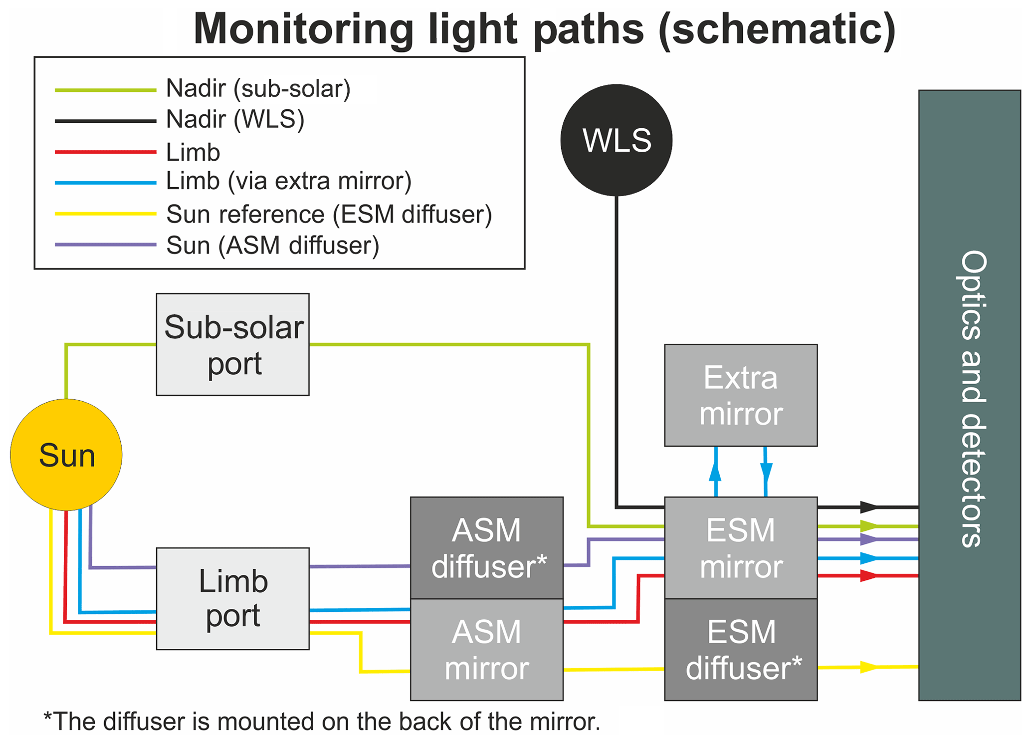
Figure 1Schematic diagram of SCIAMACHY's scanner unit with all light paths relevant for the recalibration of the solar spectra. The nadir light path provides solar measurements via the sub-solar port and ESM mirror, the limb light path solar measurements via the limb port and both scan mirrors. There is also the option of using an extra mirror in this light path. The nominal solar reference measurements (Sun reference, absolute radiometrically calibrated) use the ESM diffuser and the ASM mirror as light path. Solar measurements via the ASM diffuser and the ESM mirror are also possible. In-flight monitoring and wavelength calibration are done using the WLS and the spectral line source (SLS, not shown), respectively.
2.3 Calibration
The calibration of SCIAMACHY solar measurements includes the following steps (Slijkhuis and Lichtenberg, 2018): detector corrections address the pixel-to-pixel gain (diode arrays), the memory effect in the UV and visible channels (residual signal from the previous detector readout), and the nonlinearity effect of the NIR detectors. Dark signal corrections are based on dark current measurements performed during the night-time of each orbit. Furthermore, a stray light correction and polarisation correction that accounts for the polarisation sensitivity of the instrument were applied (Lichtenberg et al., 2006). SCIAMACHY's spectral calibration uses in-flight measurements of atomic spectral lines from the internal spectral line source (SLS), a Pt/Cr–Ne hollow cathode lamp (Slijkhuis and Lichtenberg, 2014). The absolute radiometric calibration uses on-ground calibrations that were carried out pre-flight using a combination of spectralon or NASA sphere and FEL lamps (filament emission lamp). The radiometric calibration accounted for the scan angle dependence of the signal, since the reflectivity of mirrors and diffusers changes with the incidence angle. Changes in calibration parameters due to the transition of the instrument from pre-flight to in-orbit conditions were adjusted by an on-ground to in-flight correction, as described in Hilbig et al. (2018). A degradation correction determined using in-flight measurements is applied to account for instrument throughput changes during the mission lifetime (see Sect. 3).
3.1 Starting point: in-flight degradation correction approaches for SCIAMACHY
The general idea of the degradation correction for the SCIAMACHY instrument is to use a combination of measurements from different monitoring light paths to identify changes in the optical components (diffuser and mirror transmission changes).
The first version of a degradation correction was developed from the monitoring of the instrument and applied for SCIAMACHY V7 level 1 products (solar irradiance and backscattered radiances) (e.g. Bramstedt et al., 2009). Ratios of solar and white light source (WLS) monitoring measurement (see Fig. 1) with respect to initial measurements from 2 August 2002 (beginning of SCIAMACHY measurements) were determined for the various optical paths. The time series of the ratios are the so-called monitoring factors (m-factors) and can be used for the degradation correction. This approach does not distinguish between degradation and natural variability in solar radiation. Therefore any trend information in SCIAMACHY SSI is lost.
For SCIAMACHY V8 a more sophisticated approach was introduced and revised in V9. The scanner unit (mirrors and diffusers; see Fig. 1) is described by a physical model (Krijger et al., 2014; Bramstedt, 2014). The model uses the Mueller matrix formalism and Fresnel equations to describe the different light paths and optical elements in the scanner unit (for details, see Krijger et al., 2014). The approach follows the hypothesis that mirrors and diffusers degrade by the deposition of a thin absorbing layer of contaminants that changes with time. Thus, the thickness and optical properties of the contamination layer on the mirrors and diffusers are used as a fit parameter within the scanner model. The scanner unit is followed by the optical bench module (OBM, including telescope, spectrometer, and detectors) that is common for all light paths. Consequently, the OBM transmission change is described by a single, wavelength-dependent degradation factor (OBM m-factor). Parameters (contamination layer thicknesses and properties, OBM m-factor) are fitted from ratios of in-flight calibration measurements (degradation modelling) using the combination of available light paths.
An initial approach to account for solar variability was introduced with V9. The degradation model now includes additional natural variability terms using solar proxies (Mg II index and F10.7 cm radio flux) as auxiliary fitting parameters. The impact of sunspot darkening was neglected to a first order.
The degradation correction only accounts for degradation changes since the first measurements in space. For SCIAMACHY V9, the reference day of the degradation correction was set to 27 February 2003. All calibration change from pre-launch until the reference date for the in-flight degradation correction are assumed to be accounted for by the on-ground to in-flight correction (Hilbig et al., 2018) that was introduced with V9.
The degradation correction works well in general, but there are some issues in the final phase of the mission (after 2009) and the early period in 2002. It provided a reasonably stable solar spectrum that is sufficient for most atmospheric applications but requires modifications for solar applications, e.g. studies of solar variability.
3.2 Modifications for solar applications
The degradation correction applied in V9.01 was not sufficient for studies on SSI variability and trends due to the challenges encountered to separate natural and instrumental changes adequately. It also did not work well in the final phase of the mission after 2009 and the early period during 2002. In addition some short time seasonal patterns remained in the time series and artefacts were visible for the first few days following non-nominal decontaminations, e.g. in August 2003, December 2004, and December 2008. For solar applications, modifications of the degradation model are needed.
The following issues arise in the current degradation correction. Firstly, for operational reasons, the sub-solar measurements (see Fig. 1) were not made in 2002. As a result the OBM m-factors before February 2003 were calculated assuming fixed settings for the contamination layers (as defined at the reference day in February 2003) and a constant Sun for the ESM diffuser light path. Additionally, temperature settings of the instrument were changed in February 2003. An additional solar light path uses an extra mirror such that the light crosses the ESM mirror twice. The extra mirror is small and covers only a part of the solar disc in contrast to all other light path measurements. Overall, there are basically two types of direct solar observations made by SCIAMACHY. The first involves a diffuser, which scatters the solar light into a diffuse beam with some loss of intensity; the second uses a small aperture to reduce the amount of incoming light. The limb, sub-solar, and extra-mirror light paths (Fig. 1) belong to the latter type. The observations via a small aperture cause additional diffraction effects. Hence, for an optimisation of the degradation correction, small-aperture data (type 2) are now excluded from the new degradation modelling. Only solar measurements via a diffuser are selected. ESM diffuser solar measurements (nominal solar spectra) remain part of the model and solar measurements via ASM diffuser and ESM mirror are added here. This new degradation correction modifies the scanner or mirror model and includes an updated calibration of the scan angle dependence from in-flight measurements (see Sect. 3.3 below).
In addition to the solar measurements, WLS measurements are included. The WLS is an independent light source, and therefore its measurements allow for a (better) separation of natural solar variability from instrument variations. To use these measurements in the degradation modelling, the change in the WLS with accumulated burning time needs to be properly characterised (see Sect. 3.4).
3.3 ASM diffuser solar measurements
During the on-ground calibration of SCIAMACHY, spectral features caused by the ESM diffuser were detected that were impeding atmospheric trace gas retrievals. In order to obtain a solar spectrum without these features it was necessary to add an additional diffuser with optimised optical properties on the back of the ASM mirror assembly (Gottwald and Bovensmann, 2011). This enabled regular ASM diffuser solar measurements to be made. Due to time constraints an absolute radiometric calibration for this second diffuser was not possible before launch.
The light path of the ASM diffuser measurements uses the limb port, the ASM diffuser and the ESM mirror (Fig. 1). The scanner model approach of the recent radiometric calibration for SCIAMACHY does not yet include the ASM diffuser light path. The scanner model needs the incidence angles on the optical surfaces and the relative orientations along the light path. In SCIAMACHY the detector and both scanning mechanism are in one plane with the rotation axes perpendicular to each other (Fig. 2). This geometry simplifies the calculation of the involved angles (see details in Krijger et al., 2014). In the model, a diffuser is described as a roughened surface with tiny mirror facets. Only those facets with an orientation for a specular reflection into the instrument contribute to the signal. The polarisation behaviour of a diffuser is described by a Mueller matrix for a mirror with the orientation of the reflecting facets. This orientation and the rotation angle for the Stokes vector frame from the ASM diffuser facet to the ESM mirror are calculated numerically using analytic geometry. Inputs are the direction towards the Sun (defined by the solar zenith and azimuth angle) and the direction towards the ESM mirror (defined by the rotation angle of the ESM) as shown in Fig. 3a.

Figure 2Sketch of SCIAMACHY's scanner unit with the light path for an ASM diffuser measurement. From the solar direction (defined by solar zenith and azimuth angles, SZA and SAA), the light first reaches the ASM diffuser. A small fraction of the light is scattered towards the ESM mirror such that the ESM mirror reflects the light into the telescope.

Figure 3(a) Only the ASM diffuser facets with an orientation for a specular reflection towards the ESM mirror contribute to the measured signal. The orientation of these facets is calculated from the direction towards the Sun and the ESM mirror using analytic geometry. (b) The diffuser sensitivity depends on the incident angles of the solar direction and the direction towards the ESM mirror and the azimuth angle between these two.
The diffuser sensitivity depends on the incidence angles of the incoming irradiance, the outgoing beam towards the telescope via the ESM mirror, and the azimuth angle between these directions (Fig. 3b).
One ASM diffuser measurement comprises a sequence of 30 individual measurements. The ASM diffuser is rotated by 12∘ during the sequence to further minimise spectral features in the mean spectrum. Additionally, the observing geometry towards the Sun varies over the year, which leads to five different ranges for these rotations over the year. A closer look shows that all possible geometries are covered in a time range from mid-February to the end of May. The ESM mirror stays at a fixed angle; therefore two of the three angles are sufficient to parameterise the diffuser sensitivity. We choose the incident angle from the solar direction and the azimuth angle. The degradation itself as well as the degradation rate is lowest in the early phase of the mission. Therefore, Sun–Earth-distance-normalised in-flight measurements from February to March 2003 are used to generate a wavelength-dependent look-up table (LUT) for the diffuser sensitivity.
Figure 4 visualises an example of the LUT. The LUT normalises each individual ASM diffuser measurement to the diffuser sensitivity of the reference measurement. The normalisation factors are in the range of ±40 %. After this normalisation, the differences between the individual readouts of a measurement sequence are well below 0.5 %.
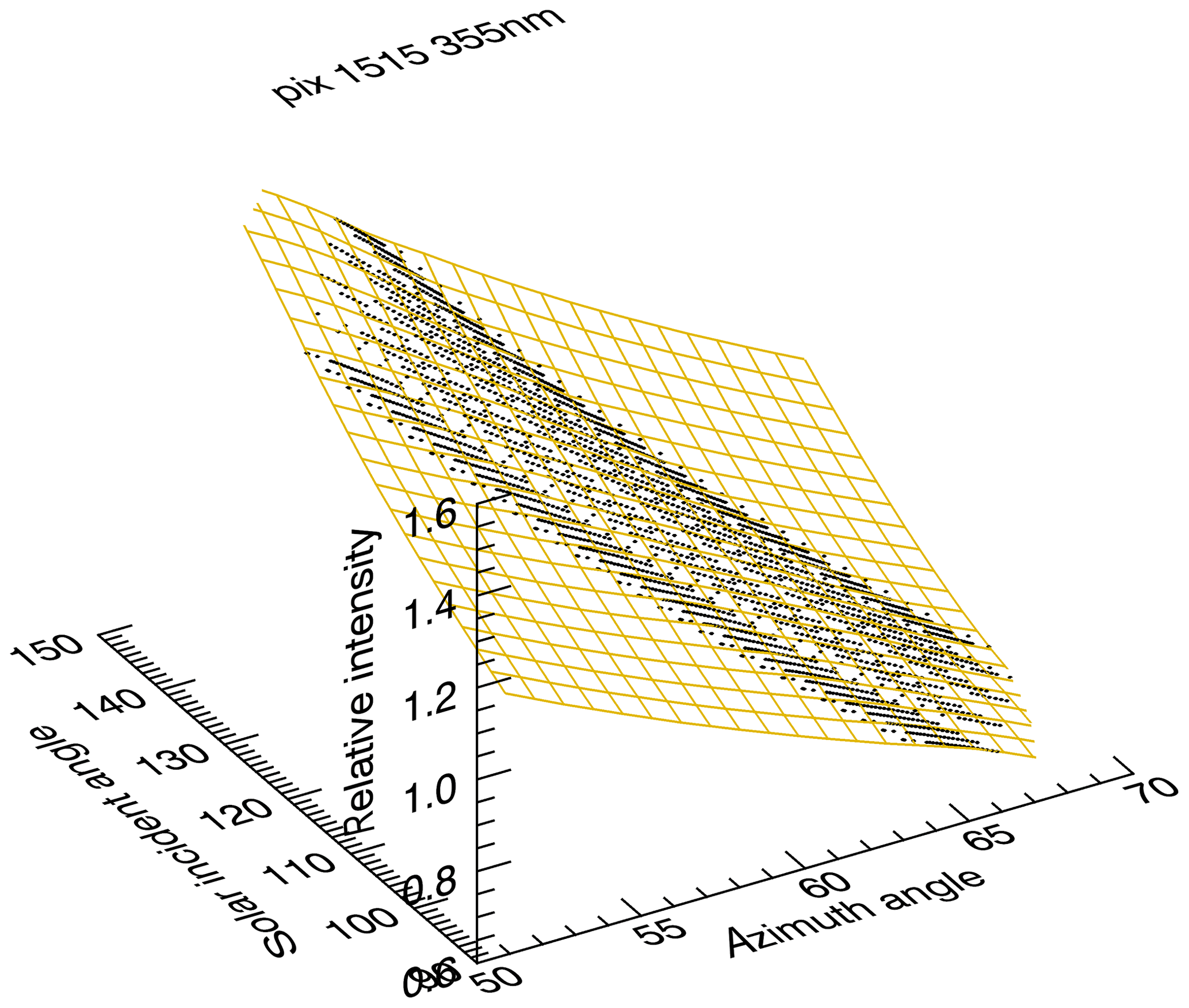
Figure 4Visualisation of a look-up table (LUT) for the ASM diffuser sensitivity. The LUT for 355 nm (in channel 2) is shown. The black dots are the measured intensities, relative to the reference measurements (15th readout on 27 February 2003). The overlay is the interpolated LUT. The LUT values depend on the incident angle of the solar irradiance and the azimuth angle between the solar and the ESM incidence angles.
On 26 May 2003, the tangent height for the dark current measurements of the limb measurement were changed by up-dating a so-called timeline of the instrument. This change had an unintended side effect for the ASM diffuser measurement: the fixed position of the ESM mirror during the ASM diffuser measurement was changed by about 1∘, which alters the range of possible geometries. Therefore, a second LUT has been generated from the measurements in mid-February to the end of May 2004 to normalise the measurements since 26 May 2003.
With the integration into SCIAMACHY's scanner model and the calibration of the diffuser sensitivity from in-flight measurements, we provide a radiometric calibration for the ASM diffuser measurements relative to the reference measurement.
3.4 WLS ageing correction
SCIAMACHY's internal WLS is a 5 W UV-optimised Tungsten halogen lamp. Its primary role is to determine the pixel-to-pixel gain, check the overall throughput of the instrument, and correct wavelength-dependent effects (e.g. etalon effect, quantum efficiency). The WLS has been used already during the calibration activities on-ground and during the commissioning phase after launch. In nominal operation, the regular WLS measurements are performed weekly. In between, further WLS monitoring measurements using different optical elements in the light path are performed. Each nominal WLS measurement has a burning time of 12 s with the last 4 s used as measurement signal.
In the new degradation model, the WLS is used as an independent second light source. Before these measurements can be used in the degradation model, the “ageing” of the WLS itself has to be corrected so that the WLS can be considered to be a constant light source.
Our assumptions regarding the WLS behaviour use the understanding and knowledge gained from a detailed study by Sperling et al. (1996) at the Physikalisch-Technische Bundesanstalt (PTB). Lamps, similar to the WLS used in SCIAMACHY, show some typical ageing in the beginning until a more stable level is reached after some accumulation of burning time. Figure 5 shows as an example the change in WLS signal at 630 nm with accumulated burning time in space. For the most part, the time series follows an exponential law (see the blue line in Fig. 5). The WLS change with accumulated burning time tB can be parameterised with the following function:
where SWLS is the relative WLS signal with respect to the signal at the reference date of the degradation correction (27 February 2003). However, the time series indicate some deficits in the calibration for the early phase of the mission (2002) and the last years of operation (2009–2012). Therefore, only the red marked period of the time series is used in a non-linear least-square fit. The fit result (light blue curve in Fig. 5) gives the theoretically expected ageing of the WLS with time and is used to correct the WLS signal accordingly. This ageing of the WLS is highly spectrally dependent and happens faster for shorter wavelengths.

Figure 5Relative WLS intensity at 630 nm as a function of its accumulated burning time in orbit. (a) WLS measurements in ESA V9.01 calibration; (b) after the final iteration of the modified degradation model. The black curve shows the WLS measurements. The (fit) range that is used to derive the parameterisation of the WLS change is indicated in red. The best fit to describe the ageing of the WLS is plotted in light blue. The corrected WLS measurements as used in the degradation model are shown in green.
This approach works well for the visible and NIR spectral range. Obtaining a similar parameterisation of the WLS change with burning time in the UV (especially below 400 nm) turned out to be more problematic. The UV time series in SCIAMACHY V9.01 are not sufficiently corrected for instrument degradation to define an adequate fit range. Therefore, it is not possible to obtain the parameterisation of the WLS ageing directly by fitting an exponential law (Eq. 1). The parameters p0, p1, and p2 received from fits in the visible and NIR were extrapolated to smaller wavelengths, which led to a first approximation for the WLS ageing parameterisation in the UV spectral range and enables us to extend the WLS ageing correction down to 330 nm (SCIAMACHY channel 2).
Remaining residual features in the ageing-corrected WLS time series show uncorrected degradation effects that originate from other optical elements in the light path. In order to account for them, an iterative approach was used by repeating the WLS ageing parameterisation after the optimised overall degradation correction as described in the next section.
3.5 Iterative degradation fit
A new set of parameters to describe the instrument degradation was derived by fits of in-flight measurements. In the optimised version of the degradation model, solar measurements via ESM diffuser as well as measurements using the ASM diffuser (see Sect. 3.3) were included. Furthermore, the internal WLS represents a second independent light source. Its measurements were corrected for lamp ageing beforehand (see Sect. 3.4).
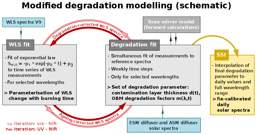
A sketch of the modified degradation modelling is shown in Fig. 6. The fit of new degradation parameters (here contaminant layer thicknesses and OBM m-factors) is performed in weekly steps based on the sampling of the WLS measurements and only for selected wavelengths. The scanner unit model (Krijger et al., 2014) is used in the forward calculations. All three measurements (ESM diffuser, ASM diffuser, WLS) are fitted simultaneously. The derived parameters are time series of the contamination layer thicknesses of the ESM mirror, ASM mirror, and ASM diffuser as well as the OBM degradation factors (summarising all spectrometer transmission and detector changes). An initial guess and first approximation of these parameters are the m-factors derived from the ESA V9.01 calibration. Following the experience from the V9.01 correction, the contaminant layer on the ESM diffuser is regarded as constant and the small ESA V9.01 value from the reference date (27 February 2003) is used for all time steps.
The results of the first degradation fit are used to repeat the WLS fit (see Sect. 3.4). With the second set of ageing-corrected WLS spectra, a second degradation correction is generated and so on. After the first iteration of the new degradation modelling, the results are already quite close to the final ones. After three iterations of WLS fitting and subsequent degradation modelling, the final results are obtained.
Fig. 5b shows the performance of the WLS ageing correction after the final iteration. The seasonal variations are much smaller and the WLS measurements later than 2008 now clearly follow the expected curve. Figure 7 shows the variation in the contamination layer thicknesses for the relevant elements of the scanner unit (see Fig. 1) over the SCIAMACHY mission lifetime. The OBM degradation factor and its changes are illustrated in Fig. 8 by some selected wavelengths from UV to NIR. The OBM mostly degrades in the UV (SCIAMACHY spectral channels 1 and 2) and the NIR (channel 6). One prominent jump in the time series at the beginning of 2009 has its origin in an ice decontamination period in December 2008. In addition, the corresponding values of SCIAMACHY V9.01 are shown as dashed or thin lines in the background of each graph. The uncertainties in the individual degradation parameters are derived within the fit procedure and indicated in the figures. Large fluctuations as well as the highest uncertainties in the degradation parameter arise in the last years starting with 2010. Therefore, comparisons of the resulting SCIAMACHY solar spectral irradiance time series with other measurements and model reconstructions include only data before 2010.
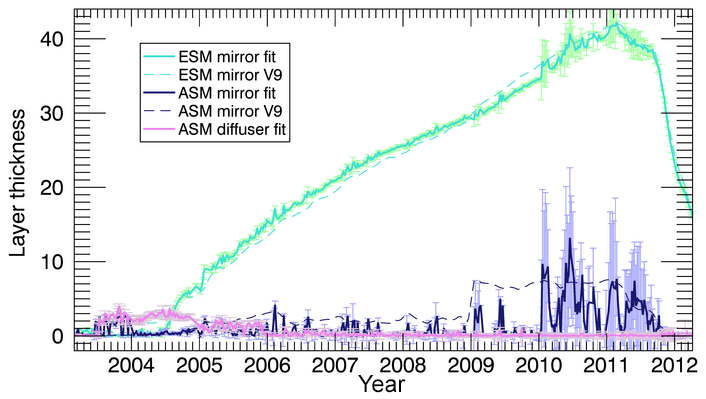
Figure 7Contamination layer thicknesses of the ESM mirror, ASM mirror, and ASM diffuser as a function of time (mission lifetime in orbit). For each optical element, two data sets are shown: dashed lines indicate the layer thicknesses of the ESA V9.01 degradation correction, and bold lines (including error bars) show the layer thicknesses derived with the modified degradation model from this study.
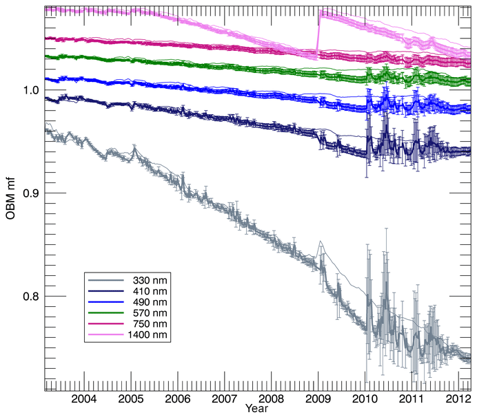
Figure 8OBM m-factors for some wavelengths as a function of time (mission lifetime in orbit). For each wavelength, two data sets are shown: thin lines indicate values from the ESA V9.01 degradation correction, and thick lines with error bars show the results from the modified degradation model from this study. The time series are vertically shifted for better visibility.
The final set of degradation parameters is interpolated to daily values and in the case of the wavelength-dependent OBM degradation factors to the SCIAMACHY spectral scale (identical with V9.01) between 320 and 1600 nm. Due to the Wood anomaly feature around 350 nm (Liebing et al., 2018), the spectral range 340–360 nm was omitted in the fit and only two wavelengths, 330 and 370 nm, for SCIAMACHY's spectral channel 2 (300–400 nm) were included. The total available wavelength range was defined firstly by the limit in deriving the WLS ageing correction which was only possible starting from 330 nm. Secondly, wavelengths above 1600 nm (SCIAMACHY channels 6+, 7, and 8) were not used in the optimised degradation modelling. Remaining uncorrected short time seasonal patterns and instrument degradation increase above 1600 nm. Since the impact of changing contamination layer thicknesses is low in this wavelength range, the inclusion in the degradation modelling could induce artefacts in the resulting degradation parameter. The newly derived parameters are then applied to recalibrate the SCIAMACHY SSI measurements.
The optimised degradation correction is used to recalibrate the SCIAMACHY solar spectral irradiances in the wavelength range 320–1600 nm. Figure 9 shows time series of SCIAMACHY solar spectra at selected wavelengths. The solid lines are recalibrated SSI data from this work, and for comparison the solar spectra of SCIAMACHY ESA V9.01 are drawn as dashed lines. With respect to ESA V9.01, a general improvement can be seen in the time series, especially for measurements after 2008. The new results show a more stable signal in the NIR with less small-scale structure. Reasonable results are also obtained in the UV near 330 nm. Here ESA V9.01 shows variations that cannot be attributed to natural solar variability, while our results show more clearly the continuous decrease as expected from the descending phase of solar cycle 23 with a clear minimum at 2008/09 as evident from other SSI measurements (e.g. Mauceri et al., 2018). However, the values are higher than expected from TSI variability (∼0.1 % solar cycle; Kopp, 2016). Furthermore, an unexpected anti-cyclic increase during solar minimum, similar to the behaviour of V9.01, becomes evident in the NUV and above; see further discussion and comparisons with other SSI data sets in Sect. 5.
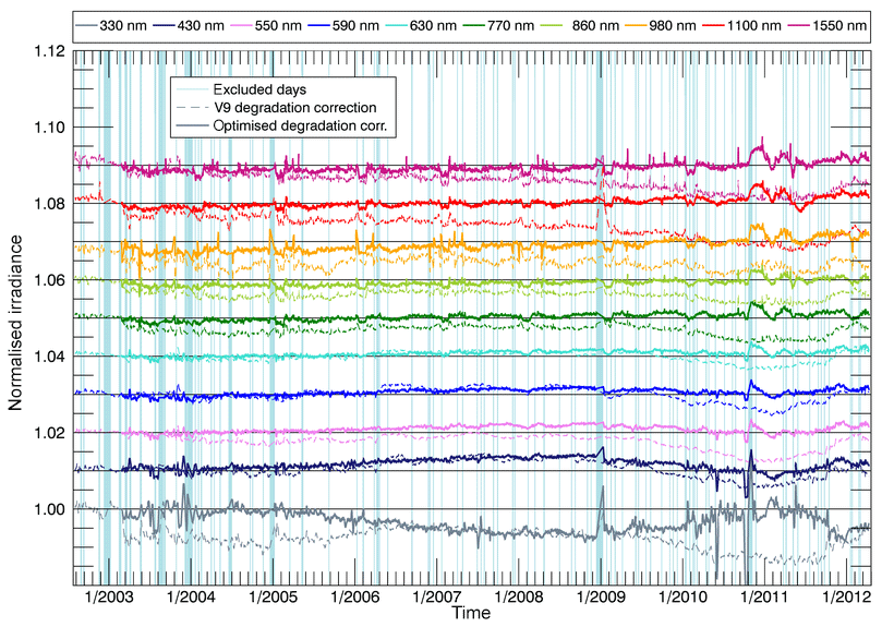
Figure 9SCIAMACHY SSI time series for selected wavelengths. Each time series is shifted vertically by 0.01 for better visibility and normalised to the reference day of degradation correction (27 February 2003). The dashed lines show the SCIAMACHY SSI with ESA V9.01 calibration; solid lines show the recalibrated SCIAMACHY SSI from this work. Vertical bars indicate days or extended periods with maintenance activities (e.g. ice decontamination periods), platform and instrument anomalies, and orbit control manoeuvres when data are considered highly uncertain.
Some new artefacts are visible, e.g. at the beginning of 2011. They seem to originate in the ASM diffuser solar spectra and are transferred to the ESM diffuser solar spectra and WLS spectra through their simultaneous fit in the degradation modelling. Besides, a beginning recovery of the instrument throughput was recorded, which is not fully understood. A possible explanation is the additional permanent use of a backup system after an anomaly in the Ka-band antenna subsystem. About 120 W more energy was dissipated resulting in a change in the thermal environment of Envisat. Increased temperatures (0.3–2.7 ∘C, subsystem-dependent) were observed by SCIAMACHY's internal temperature sensors (Gottwald et al., 2016). This changes the outgassing and thus the photochemical processing. At about the same time, the orbit of Envisat was lowered in October 2010. As a consequence, we attribute the higher variability and larger uncertainties in the degradation parameters during the final phase of the mission to the combination of these effects and the advanced ageing of the instrument. Therefore, it is challenging to generate a reasonable degradation correction for the last phase of the mission.
The recalibrated SCIAMACHY SSI were compared to other measurements from satellites that have been briefly described in the Introduction. In addition, our data were also compared with semi-empirical SSI reconstructions that are currently favoured in climate model simulations (Matthes et al., 2017). The SSI reconstructions are briefly described in the following before the results of the SSI comparisons are presented and discussed.
5.1 SSI reconstructions
An alternative to long-term SSI observations are estimates of long-term solar variations from measurements of shorter periods (e.g. a few solar rotations) by establishing information about long-time variations from extrapolation in time of fitted solar proxies, like the sunspot number, Mg II index, or 10.7 cm radio flux. Wavelength-dependent scaling factors of the solar proxies can then be used to determine SSI changes (e.g. Lean et al., 1997; Morrill et al., 2011; Pagaran et al., 2009, 2011). The Mg II index is strongly correlated with SSI changes in the near and extreme UV on timescales of the 27 d solar rotation and the 11-year solar cycle. It is thus a common solar proxy for UV SSI variability (e.g. Viereck et al., 2001; Dudok de Wit et al., 2009; Snow et al., 2014) and often used to describe solar forcing in the upper atmosphere. Another key indicator of solar magnetic activity is the total area of sunspots. The radiometric effect of sunspot passages across the solar disc can be quantified by the photometric sunspot index (PSI) (Balmaceda et al., 2009). A more complex approach by combining results from solar proxy models and solar atmosphere modelling is employed in the Naval Research Laboratory's (NRL) solar irradiance variability model, namely NRLSSI2 (Coddington et al., 2016). Another class of models uses semi-empirical models of the solar atmosphere to calculate the brightness of different surface features (such as sunspots, faculae, plage). An example is SATIRE-S (Spectral And Total Irradiance REconstructions for the satellite era), which derives the surface area coverage of the individual photospheric components by full-disc intensity images and magnetograms (Yeo et al., 2014).
5.2 SSI time series
For comparisons with the recalibrated SCIAMACHY SSI, we use the most recent data versions of SATIRE-S,2 SIM,3 and OMI.4 SIM obtains daily solar spectra from 240 to 2400 nm at a variable spectral resolution of 1 to 34 nm with an absolute uncertainty of 2 % and long-term repeatability of less than 0.1 % (Harder, 2019). Before any comparisons were performed, as shown in Figs. 10 and 11, outliers are removed from SIM V25 time series. OMI provides daily solar spectra in the 265–500 nm range of mid-resolution (0.4–0.6 nm) with an absolute accuracy of better than 4 % and high instrument stability. The optical degradation rate ranged from 0.2 to 0.5 % yr−1 (Marchenko et al., 2016, and references therein). The authors note that the current values underestimate the solar cycle variability by ∼0.1 % in the UV (<350 nm) and <0.05 % in the visible; this originates in the applied degradation correction approach.
Figure 10 shows SSI time series for several wavelength bands. Measurements from different instruments and model reconstructions are compared with SCIAMACHY SSI. The data are normalised to a reference date during solar minimum condition (5 October 2008). The solar cycle minimum occurred by the end of 2008/beginning of 2009. We choose this specific date as it lies within a period of stable SCIAMACHY measurements where uncertainties are smaller than in early 2009. The panels show the data starting with the reference date of SCIAMACHY degradation correction (27 February 2003) until the end of 2009. As discussed in Sect. 4 and shown in Figs. 7 and 8 the degradation modelling had larger uncertainties after 2009 when instrument degradation became more prominent. For our comparisons between different data sets, we focus in the following on the descending phase of solar cycle 23 until the end of 2009.
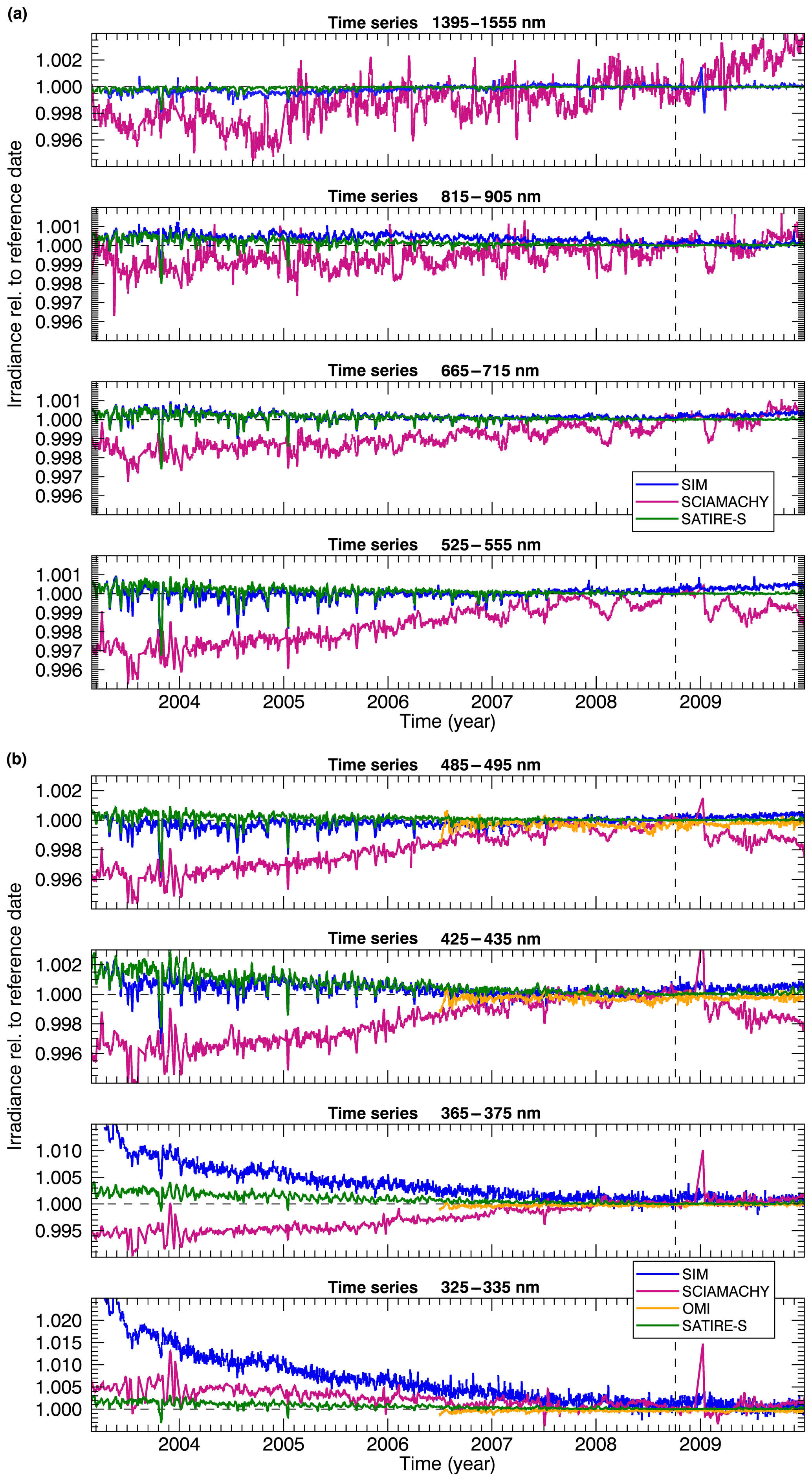
Figure 10Time series of SSI, integrated into (b) 10 nm and (a) 30–160 nm wide wavelength bands from SCIAMACHY, SIM/SORCE V25, OMI/AURA satellite measurements, and SATIRE-S. The time series are ratioed to values from 5 October 2008, which are representative of solar minimum conditions. For details, see text. (Note the change in vertical scale for the different wavelength ranges.)
Beginning with the lowest wavelength band centred at 330 nm, the SCIAMACHY SSI time series lies within the solar cycle variation in SATIRE-S and SIM V25 data sets. It shows the expected minimum at the time of solar activity minimum in accordance with the other SSI data. Nevertheless large differences in comparison to SIM become obvious in the UV. This was previously reported by studies, e.g., Haberreiter et al. (2017), Mauceri et al. (2018), and Coddington et al. (2019); these point to comparably large solar cycle variability results for recent SSI from SIM in the UV. For higher wavelengths in the UV and visible spectral range (starting at 370 nm in Fig. 10) SCIAMACHY shows an increasing signal towards solar minimum and a decrease afterwards. This would imply anti-correlation of the solar irradiances in the visible and the 11-year solar cycle. Similar results were published earlier for SIM (Harder et al., 2009; Haigh et al., 2010) but are inconsistent with other satellite measurements that show in-phase variations (Wehrli et al., 2013; Marchenko and DeLand, 2014). Recent studies by Woods et al. (2018) and Mauceri et al. (2018) developed new methods to account for uncorrected degradation in SIM SSI. Both results, the MuSIL-corrected SIM and SIMc, show better agreement with independent SSI data such as SATIRE-S than the operational SIM product (Harder, 2019). The observed anti-correlation for the new SCIAMACHY results is therefore likely a remaining residual instrument artefact. For the time series in the NIR above 1000 nm (SCIAMACHY channel 6) the overall increase agrees qualitatively with the SIM observations, but the rate of increase is higher than compared to SIM and SATIRE-S. OMI generally shows good agreement with SATIRE-S and, therefore, strengthens its role as a reference for SSI comparisons. Unfortunately, the degradation-corrected data set starts in July 2006 and is not available for the first part of the mission when solar activity was stronger.
It seems that for most parts of the visible and near-IR spectral range a remaining positive drift, most likely instrumental in nature, is evident in the SCIAMACHY time series that is on the order of +1 % per decade. The SCIAMACHY mission was accompanied by a high number of instrument and platform anomalies as well as many regular maintenance activities as illustrated by blue lines in Fig. 9. These anomalies and maintenances mostly had minimal impact on atmospheric trace gas retrievals, the primary purpose of SCIAMACHY, but have a non-negligible impact on the degradation correction and radiometric stability. One of the most important maintenance activities were decontamination periods where the detectors were heated to remove ice contamination of the NIR detectors, but they also impacted the UV and visible spectral bands.
In 2004, larger short time variations are visible in the SCIAMACHY time series. At the beginning of the mission the contamination layers are still faint and the resulting degradation effect small. Therefore it is more difficult to determine the degradation parameter in the degradation modelling. That is further hindered by ice decontamination periods that were included in the instrument operation more frequently at the beginning of the mission.
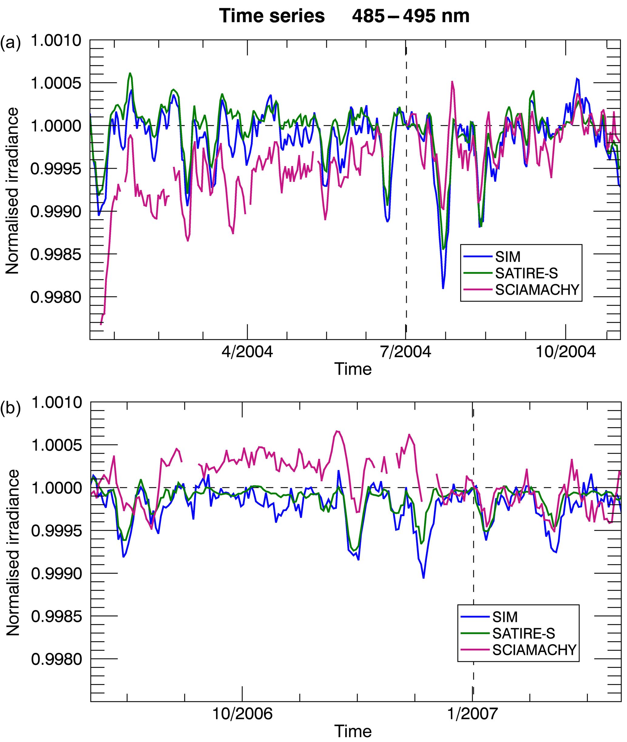
Figure 11Time series of SSI, integrated into a 10 nm wide wavelength band from SCIAMACHY, SIM/SORCE V25, and SATIRE-S. The figure provide a detailed view of 10-month periods in 2004 (a) and 2006/07 (b). The time series are ratioed to values from 1 July 2004 and 1 January 2007, respectively, to shift the data sets for better comparability.
On smaller timescales (solar rotations), SCIAMACHY follows most of the prominent signatures in the time series; see Fig. 11. Up to about 700 nm SCIAMACHY shows a realistic decrease in the amplitude of variations from higher solar activity towards the minimum.
Despite a clear improvement of the SCIAMACHY SSI in comparison with ESA V9.01, as discussed in Sect. 4, the current degradation correction is not yet sufficient to account for all instrumental effects, such as the remaining positive drift in the SSI time series. Further work is required to clarify the origins of differences between SCIAMACHY and other SSI data sets. Nevertheless, we were able to show that the WLS in the new degradation correction scheme significantly contributes to improvements in the in-flight radiometric calibration.
One of the main limitations for long-term space-based measurements is the optical degradation of the instrument due to the harsh environment of space operation. Therefore, a thorough degradation correction to maintain instrument calibration for the instrument's lifetime is required. In this paper, we presented a modification of SCIAMACHY's degradation correction approach (Krijger et al., 2014), which models (growing) contamination layers on the optical surfaces in the scanner unit of the spectrometer responsible for instrumental throughput losses with space mission time. Changes in the optical components (diffuser and mirror transmission changes) were identified using a combination of solar measurements from different monitoring light paths. In this work the set of solar monitoring measurements to be included in the degradation modelling was changed. Solar measurements via a second diffuser (ASM diffuser) are now included in the model, after new scan-angle-dependent transmission changes were introduced. The second essential part of the modification is the inclusion of measurements from SCIAMACHY's internal white light source. Including the WLS as a second and independent light source provided the opportunity to better separate instrument variations and natural solar variability.
Before the WLS measurements could be used in the degradation model, emission changes in the WLS had to be accounted for. The change in the WLS emission as a function of accumulated burning time was successfully determined and was found to be qualitatively consistent with detailed lamp studies by Sperling et al. (1996) at the PTB. An iterative approach of WLS correction and subsequent spectrometer degradation modelling was successfully implemented.
A general improvement over the current SCIAMACHY ESA V9.01 SSI was found, but there are still limitations in the degradation corrections, particularly in the late period between 2010 until the end of the satellite mission in 2012. Due to the numerous instrument and platform anomalies as well as intended decontamination phases to sublime the ice layer on the SCIAMACHY detectors, the degradation corrections were not sufficient to remove all artefacts and small drifts in the SCIAMACHY SSI time series.
The main achievement of this study was the successful characterisation of the WLS ageing and the integration of the WLS measurements in the existing degradation model. This will provide an important contribution for a revised degradation correction in possible future data products by ESA. This study showed the potential of an internal WLS for degradation monitoring of other satellite instruments such as GOME-2, OMI, and TROPOMI, which also include this type of lamp.
The newly derived SCIAMACHY SSI data set is available at http://www.iup.uni-bremen.de/UVSAT/datasets/scia-ssi-timeseries (last update: July 2020, Hilbig et al., 2020). Please note that there are still limitations in the degradation correction and not all calibration issues were solved. At the time of writing, the SCIAMACHY SSI data set covers the wavelength range from 320 to 1600 nm and contains gaps at SCIAMACHY spectral channel boundaries and around 350 nm. SCIAMACHY provided daily measurements with short interruptions during satellite and instrument maintenance periods. Possible updates will be provided and announced on the web page.
TH investigated the WLS ageing and performed the iterative degradation fit. KB implemented the ASM diffuser solar measurements in the scanner model. Comparisons of SSI data sets were done by TH with collaboration by MW. MK contributed the scanner model. KB and MK developed previous degradation corrections, on which this work is based on. TH prepared the manuscript with contributions from all co-authors (including JPB).
The authors declare that they have no conflict of interest.
SCIAMACHY is a national contribution to the ESA Envisat project, funded by Germany, The Netherlands, and Belgium. The authors thank ESA for providing the SCIAMACHY data and the SCIAMACHY Quality Working Group for their work on SCIAMACHY level 1 data. The support from the SCIASOL project under the BMBF priority programme ROMIC (Role of the Middle Atmosphere in Climate) and the University of Bremen is gratefully acknowledged.
The article processing charges for this open-access publication were covered by the University of Bremen.
This paper was edited by Saulius Nevas and reviewed by Martin Snow and two anonymous referees.
Balmaceda, L. A., Solanki, S. K., Krivova, N. A., and Foster, S.: A homogeneous database of sunspot areas covering more than 130 years, J. Geophys. Res., 114, A07104, https://doi.org/10.1029/2009JA014299, 2009. a
BenMoussa, A., Gissot, S., Schühle, U., Del Zanna, G., Auchère, F., Mekaoui, S., Jones, A. R., Walton, D., Eyles, C. J., Thuillier, G., Seaton, D., Dammasch, I. E., Cessateur, G., Meftah, M., Andretta, V., Berghmans, D., Bewsher, D., Bolsée, D., Bradley, L., Brown, D. S., Chamberlin, P. C., Dewitte, S., Didkovsky, L. V., Dominique, M., Eparvier, F. G., Foujols, T., Gillotay, D., Giordanengo, B., Halain, J. P., Hock, R. A., Irbah, A., Jeppesen, C., Judge, D. L., Kretzschmar, M., McMullin, D. R., Nicula, B., Schmutz, W., Ucker, G., Wieman, S., Woodraska, D., and Woods, T. N.: On-orbit degradation of solar instruments, Sol. Phys., 288, 389–434, https://doi.org/10.1007/s11207-013-0290-z, 2013. a, b, c
Bovensmann, H., Aben, I., van Roozendael, M., Kühl, S., Gottwald, M., von Savigny, C., Buchwitz, M., Richter, A., Frankenberg, C., Stammes, P., de Graaf, M., Wittrock, F., Sinnhuber, M., Sinnhuber, B.-M., Schönhardt, A., Beirle, S., Gloudemans, A., Schrijver, H., Bracher, A., Rozanov, A. V., Weber, M., and Burrows, J. P.: SCIAMACHY's view of the changing earth's environment, in: SCIAMACHY – Exploring the Changing Earth’s Atmosphere, edited by: Gottwald, M. and Bovensmann, H., Springer, Dordrecht, chap. 10, 175–216, https://doi.org/10.1007/978-90-481-9896-2, 2011. a
Bramstedt, K.: Scan-angle dependent degradation correction with the scanner model approach, Tech. Rep. IUP-SCIA-TN-Mfactor, Version 1.0, Institute of Environmental Physics (IUP), available at: http://www.iup.uni-bremen.de/UVSAT_material/technotes/SCIAMACHY_calibration/mfactor-TN-3-1_20140428.pdf (last access: June 2020), 2014. a
Bramstedt, K., Noël, S., Bovensmann, H., Burrows, J. P., Lerot, C., Tilstra, L. G., Lichtenberg, G., Dehn, A., and Fehr, T.: SCIAMACHY monitoring factors: Observation and end-to-end correction of instrument performance degradation, in: Atmospheric Science Conference, Barcelona, Spain, 7–11 September 2009, ESA SP-676, 2009. a
Burrows, J. P., Hölzle, E., Goede, A., Visser, H., and Fricke, W.: SCIAMACHY - Scanning Imaging Absorption Spectrometer for atmospheric chartography, Acta Astronaut., 35, 445–451, https://doi.org/10.1016/0094-5765(94)00278-T, 1995. a, b
Burrows, J. P., Weber, M., Buchwitz, M., Rozanov, V., Ladstätter-Weißenmayer, A., Richter, A., DeBeek, R., Hoogen, R., Bramstedt, K., Eichmann, K.-U., Eisinger, M., and Perner, D.: The Global Ozone Monitoring Experiment (GOME): Mission concept and first scientific results, J. Atmos. Sci., 56, 151–175, https://doi.org/10.1175/1520-0469(1999)056<0151:TGOMEG>2.0.CO;2, 1999. a
Coddington, O., Lean, J. L., Pilewskie, P., Snow, M., and Lindholm, D.: A Solar Irradiance Climate Data Record, B. Am. Meteorol. Soc., 97, 1265–1282, https://doi.org/10.1175/BAMS-D-14-00265.1, 2016. a
Coddington, O., Lean, J., Pilewskie, P., Snow, M., Richard, E., Kopp, G., Lindholm, C., DeLand, M., Marchenko, S., Haberreiter, M., and Baranyi, T.: Solar Irradiance Variability: Comparisons of Models and Measurements, Earth and Space Science, 6, 2525–2555, https://doi.org/10.1029/2019EA000693, 2019. a
DeLand, M. T., Taylor, S. L., Huang, L. K., and Fisher, B. L.: Calibration of the SBUV version 8.6 ozone data product, Atmos. Meas. Tech., 5, 2951–2967, https://doi.org/10.5194/amt-5-2951-2012, 2012. a, b, c
Dudok de Wit, T., Kretzschmar, M., Lilensten, J., and Woods, T.: Finding the best proxies for the solar UV irradiance, Geophys. Res. Lett., 36, L10107, https://doi.org/10.1029/2009GL037825, 2009. a
Ermolli, I., Matthes, K., Dudok de Wit, T., Krivova, N. A., Tourpali, K., Weber, M., Unruh, Y. C., Gray, L., Langematz, U., Pilewskie, P., Rozanov, E., Schmutz, W., Shapiro, A., Solanki, S. K., and Woods, T. N.: Recent variability of the solar spectral irradiance and its impact on climate modelling, Atmos. Chem. Phys., 13, 3945–3977, https://doi.org/10.5194/acp-13-3945-2013, 2013. a, b, c, d, e
Floyd, L. E., Cook, J. W., Herring, L. C., and Crane, P. C.: SUSIM'S 11-year observational record of the solar UV irradiance, Adv. Space Res., 31, 2111–2120, https://doi.org/10.1016/S0273-1177(03)00148-0, 2003. a
Gottwald, M. and Bovensmann, H. (Eds.): SCIAMACHY – Exploring the Changing Earth's Atmosphere, Springer Netherlands, Dordrecht, https://doi.org/10.1007/978-90-481-9896-2, 2011. a, b
Gottwald, M., Hoogeveen, R., Chlebek, C., Bovensmann, H., Carpay, J., Lichtenberg, G., Krieg, E., Lützow-Wentzky, P., and Watts, T.: The Instrument, in: SCIAMACHY – Exploring the Changing Earth's Atmosphere, chap. 3, 29–46, https://doi.org/10.1007/978-90-481-9896-2, 2011. a
Gottwald, M., Krieg, E., Lichtenberg, G., Noël, S., Bramstedt, K., Bovensmann, H., Snel, R., and Krijger, M.: SCIAMACHY In-Orbit Mission Report, DLR-IMF & IUP-IFE & SRON, PO-TN-DLR-SH-0034, Issue 1, Rev 0, available at: https://atmos.eoc.dlr.de/projects/scops/ (last access: March 2020) (see: Mission Documents/In-orbit Mission Report), 2016. a
Gray, L. J., Beer, J., Geller, M., Haigh, J. D., Lockwood, M., Matthes, K., Cubasch, U., Fleitmann, D., Harrison, G., Hood, L., Luterbacher, J., Meehl, G. A., Shindell, D., van Geel, B., and White, W.: Solar influences on climate, Rev. Geophys., 48, RG4001, https://doi.org/10.1029/2009RG000282, 2010. a
Haberreiter, M., Schöll, M., Dudok de Wit, T., Kretzschmar, M., Misios, S., Tourpali, K., and Schmutz, W.: A new observational solar irradiance composite, J. Geophys. Res.-Space, 122, 5910–5930, https://doi.org/10.1002/2016JA023492, 2017. a
Haigh, J. D.: The Sun and the Earth's Climate, Living Rev. Sol. Phys., 4, 2, https://doi.org/10.12942/lrsp-2007-2, 2007. a
Haigh, J. D., Winning, A. R., Toumi, R., and Harder, J. W.: An influence of solar spectral variations on radiative forcing of climate, Nature, 467, 696–699, https://doi.org/10.1038/nature09426, 2010. a, b
Harber, D.: CSIM, available at: https://lasp.colorado.edu/home/csim/, last access: 26 August 2019. a
Harder, J.: SORCE SIM Level 3 Solar Spectral Irradiance Daily Means V025, Goddard Earth Sciences Data and Information Services Center (GES DISC), https://doi.org/10.5067/0EQZJBS6B39C, 2019. a, b, c
Harder, J., Lawrence, G., Fontenla, J., Rottman, G., and Woods, T.: The Spectral Irradiance Monitor: Scientific Requirements, Instrument Design, and Operation Modes, Sol. Phys., 230, 141–167, https://doi.org/10.1007/s11207-005-5007-5, 2005. a, b
Harder, J. W., Fontenla, J. M., Pilewskie, P., Richard, E. C., and Woods, T. N.: Trends in solar spectral irradiance variability in the visible and infrared, Geophys. Res. Lett., 36, L07801, https://doi.org/10.1029/2008GL036797, 2009. a, b
Harder, J. W., Thuillier, G., Richard, E. C., Brown, S. W., Lykke, K. R., Snow, M., McClintock, W. E., Fontenla, J. M., Woods, T. N., and Pilewskie, P.: The SORCE SIM solar spectrum: Comparison with recent observations, Sol. Phys., 263, 3–24, https://doi.org/10.1007/s11207-010-9555-y, 2010. a
Hilbig, T., Weber, M., Bramstedt, K., Noël, S., Burrows, J. P., Krijger, J. M., Snel, R., Meftah, M., Damé, L., Bekki, S., Bolsée, D., Pereira, N., and Sluse, D.: The New SCIAMACHY Reference Solar Spectral Irradiance and its Validation, Sol. Phys., 293, 121, https://doi.org/10.1007/s11207-018-1339-9, 2018. a, b, c, d, e, f
Hilbig, T., Weber, M., and Bramstedt, K.: SCIAMACHY solar spectral irradiance time series, IUP V1, http://www.iup.uni-bremen.de/UVSAT/datasets/scia-ssi-timeseries, last update: July 2020. a
Kopp, G.: Magnitudes and timescales of total solar irradiance variability, J. Space Weather Spac., 6, A30, https://doi.org/10.1051/swsc/2016025, 2016. a
Kren, A. C., Pilewskie, P., and Coddington, O.: Where does Earth's atmosphere get its energy?, J. Space Weather Spac., 7, A10, https://doi.org/10.1051/swsc/2017007, 2017. a
Krijger, J. M., Snel, R., van Harten, G., Rietjens, J. H. H., and Aben, I.: Mirror contamination in space I: mirror modelling, Atmos. Meas. Tech., 7, 3387–3398, https://doi.org/10.5194/amt-7-3387-2014, 2014. a, b, c, d, e, f, g, h, i, j
Krivova, N. A., Solanki, S. K., Wenzler, T., and Podlipnik, B.: Reconstruction of solar UV irradiance since 1974, J. Geophys. Res., 114, D00I04, https://doi.org/10.1029/2009JD012375, 2009. a
Lean, J. L.: Sun-Climate Connections, Oxford Research Encyclopedia of Climate Science, https://doi.org/10.1093/acrefore/9780190228620.013.9, 2017. a, b
Lean, J. L. and DeLand, M. T.: How does the Sun's spectrum vary?, J. Climate, 25, 2555–2560, https://doi.org/10.1175/JCLI-D-11-00571.1, 2012. a, b
Lean, J. L., Rottman, G. J., Kyle, H. L., Woods, T. N., Hickey, J. R., and Puga, L. C.: Detection and parameterization of variations in solar mid- and near-ultraviolet radiation (200–400 nm), J. Geophys. Res. Atmos., 102, 29939–29956, https://doi.org/10.1029/97JD02092, 1997. a
Levelt, P. F., van den Oord, G. H. J., Dobber, M. R., Malkki, A., Visser, H., de Vries, J., Stammes, P., Lundell, J. O. V., and Saari, H.: The Ozone Monitoring Instrument, IEEE T. Geosci. Remote, 44, 1093–1101, https://doi.org/10.1109/TGRS.2006.872333, 2006. a
Lichtenberg, G., Kleipool, Q., Krijger, J. M., van Soest, G., van Hees, R., Tilstra, L. G., Acarreta, J. R., Aben, I., Ahlers, B., Bovensmann, H., Chance, K., Gloudemans, A. M. S., Hoogeveen, R. W. M., Jongma, R. T. N., Noël, S., Piters, A., Schrijver, H., Schrijvers, C., Sioris, C. E., Skupin, J., Slijkhuis, S., Stammes, P., and Wuttke, M.: SCIAMACHY Level 1 data: calibration concept and in-flight calibration, Atmos. Chem. Phys., 6, 5347–5367, https://doi.org/10.5194/acp-6-5347-2006, 2006. a, b
Liebing, P., Krijger, M., Snel, R., Bramstedt, K., Noël, S., Bovensmann, H., and Burrows, J. P.: In-flight calibration of SCIAMACHY's polarization sensitivity, Atmos. Meas. Tech., 11, 265–289, https://doi.org/10.5194/amt-11-265-2018, 2018. a
Marchenko, S. V. and DeLand, M. T.: Solar spectral irradiance changes during cycle 24, Astrophys. J., 789, 117, https://doi.org/10.1088/0004-637X/789/2/117, 2014. a, b, c
Marchenko, S. V., DeLand, M. T., and Lean, J. L.: Solar spectral irradiance variability in cycle 24: observations and models, J. Space Weather Spac., 6, A40, https://doi.org/10.1051/swsc/2016036, 2016. a
Matthes, K., Funke, B., Andersson, M. E., Barnard, L., Beer, J., Charbonneau, P., Clilverd, M. A., Dudok de Wit, T., Haberreiter, M., Hendry, A., Jackman, C. H., Kretzschmar, M., Kruschke, T., Kunze, M., Langematz, U., Marsh, D. R., Maycock, A. C., Misios, S., Rodger, C. J., Scaife, A. A., Seppälä, A., Shangguan, M., Sinnhuber, M., Tourpali, K., Usoskin, I., van de Kamp, M., Verronen, P. T., and Versick, S.: Solar forcing for CMIP6 (v3.2), Geosci. Model Dev., 10, 2247–2302, https://doi.org/10.5194/gmd-10-2247-2017, 2017. a
Mauceri, S., Pilewskie, P., Richard, E., Coddington, O., Harder, J., and Woods, T.: Revision of the Sun's Spectral Irradiance as Measured by SORCE SIM, Sol. Phys., 293, 161, https://doi.org/10.1007/s11207-018-1379-1, 2018. a, b, c, d
McClintock, W. E., Snow, M., and Woods, T. N.: Solar-Stellar Irradiance Comparison Experiment II (SOLSTICE II): Pre-launch and on-orbit calibrations, Sol. Phys., 230, 259–294, https://doi.org/10.1007/s11207-005-1585-5, 2005. a, b
Meftah, M., Damé, L., Bolsée, D., Pereira, N., Sluse, D., Cessateur, G., Irbah, A., Sarkissian, A., Djafer, D., Hauchecorne, A., and Bekki, S.: A New Solar Spectrum from 656 to 3088 nm, Sol. Phys., 292, 101, https://doi.org/10.1007/s11207-017-1115-2, 2017. a
Meftah, M., Dominique, M., BenMoussa, A., Dammasch, I. E., Bolsée, D., Pereira, N., Damé, L., Bekki, S., and Hauchecorne, A.: On-orbit degradation of recent space-based solar instruments and understanding of the degradation processes, in: Proc. SPIE 10196, Sensors and Systems for Space Applications X, SPIE, https://doi.org/10.1117/12.2250031, 2017. a
Meftah, M., Damé, L., Bolsée, D., Hauchecorne, A., Pereira, N., Sluse, D., Cessateur, G., Irbah, A., Bureau, J., Weber, M., Bramstedt, K., Hilbig, T., Thiéblemont, R., Marchand, M., Lefèvre, F., Sarkissian, A., and Bekki, S.: SOLAR-ISS: A new reference spectrum based on SOLAR/SOLSPEC observations, Astron. Astrophys., 611, A1, https://doi.org/10.1051/0004-6361/201731316, 2018. a
Morrill, J. S., Floyd, L., and McMullin, D.: The solar ultraviolet spectrum estimated using the Mg II index and Ca II K disk activity, Sol. Phys., 269, 253–267, https://doi.org/10.1007/s11207-011-9708-7, 2011. a
Morrill, J. S., Floyd, L., and McMullin, D.: Comparison of Solar UV Spectral Irradiance from SUSIM and SORCE, Sol. Phys., 289, 3641–3661, https://doi.org/10.1007/s11207-014-0535-5, 2014. a, b
Munro, R., Lang, R., Klaes, D., Poli, G., Retscher, C., Lindstrot, R., Huckle, R., Lacan, A., Grzegorski, M., Holdak, A., Kokhanovsky, A., Livschitz, J., and Eisinger, M.: The GOME-2 instrument on the Metop series of satellites: instrument design, calibration, and level 1 data processing – an overview, Atmos. Meas. Tech., 9, 1279–1301, https://doi.org/10.5194/amt-9-1279-2016, 2016. a
Pagaran, J., Weber, M., and Burrows, J. P.: Solar variability from 240 to 1750 nm in terms of faculae brightening and sunspot darkening from SCIAMACHY, Astrophys. J., 700, 1884–1895, https://doi.org/10.1088/0004-637X/700/2/1884, 2009. a, b
Pagaran, J., Weber, M., DeLand, M., Floyd, L., and Burrows, J. P.: Solar spectral irradiance variations in 240-1600 nm during the recent solar cycles 21–23, Sol. Phys., 272, 159–188, https://doi.org/10.1007/s11207-011-9808-4, 2011. a, b
Pilewskie, P., Kopp, G., Richard, E., Coddington, O., Sparn, T., and Woods, T.: TSIS-1 and Continuity of the Total and Spectral Solar Irradiance Climate Data Record, EGU General Assembly, Vienna, Austria, 8–13 April 2018, EGU2018-5527, 2018. a
Reber, C. A., Trevathan, C. E., McNeal, R. J., and Luther, M. R.: The Upper Atmosphere Research Satellite (UARS) mission, J. Geophys. Res., 98, 10643–10647, https://doi.org/10.1029/92JD02828, 1993. a
Slijkhuis, S. and Lichtenberg, G.: SCIAMACHY L0-1c Processor ATBD (Algorithm Teoretical Baseline Document for Processor V.8), Docnr.: ENV-ATB-DLR-SCIA-0041, Issue: 6, DLR-IMF, available at: https://earth.esa.int/documents/700255/708683/ENV-ATB-DLR-SCIA-0041-6-SCIA-L1B-ATBD.pdf (last access: June 2020), 2014. a
Slijkhuis, S. and Lichtenberg, G.: SCIAMACHY L0-1c Processor ATBD (Algorithm Teoretical Baseline Document for Processor V.9), Docnr.: ENV-ATB-DLR-SCIA-0041, Issue: 7, DLR-IMF, available at: https://atmos.eoc.dlr.de/sciamachy/documents/level_0_1b/scia01b_atbd_master.pdf (last access: June 2020), 2018. a
Snow, M., Weber, M., Machol, J., Viereck, R., and Richard, E.: Comparison of Magnesium II core-to-wing ratio observations during solar minimum 23/24, J. Space Weather Spac., 4, A04, https://doi.org/10.1051/swsc/2014001, 2014. a
Solar Variability And Climate Group: SATIRE model reconstruction of total and spectral solar irradiance, Max Planck Institute for Solar System Research, https://doi.org/10.17617/1.5U, 2017. a
Solanki, S. K., Krivova, N. A., and Haigh, J. D.: Solar Irradiance Variability and Climate, Annu. Rev. Astron. Astr., 51, 311–351, https://doi.org/10.1146/annurev-astro-082812-141007, 2013. a
Sperling, A., Winter, S., Raatz, K.-H., and Metzdorf, J.: Entwicklung von Normallampen für das UV-B-Meß programm, Tech. Rep. PTB-Opt-52, Physikalisch-Technische Bundesanstalt, ISBN 3-89429-729-8, 1996. a, b, c
Thuillier, G., Foujols, T., Bolsée, D., Gillotay, D., Hersé, M., Peetermans, W., Decuyper, W., Mandel, H., Sperfeld, P., Pape, S., Taubert, D. R., and Hartmann, J.: SOLAR/SOLSPEC: Scientific Objectives, Instrument Performance and Its Absolute Calibration Using a Blackbody as Primary Standard Source, Sol. Phys., 257, 185–213, https://doi.org/10.1007/s11207-009-9361-6, 2009. a
Veefkind, J., Aben, I., McMullan, K., Förster, H., de Vries, J., Otter, G., Claas, J., Eskes, H., de Haan, J., Kleipool, Q., van Weele, M., Hasekamp, O., Hoogeveen, R., Landgraf, J., Snel, R., Tol, P., Ingmann, P., Voors, R., Kruizinga, B., Vink, R., Visser, H., and Levelt, P.: TROPOMI on the ESA Sentinel-5 Precursor: A GMES mission for global observations of the atmospheric composition for climate, air quality and ozone layer applications, Remote Sens. Environ., 120, 70–83, https://doi.org/10.1016/j.rse.2011.09.027, 2012. a
Viereck, R., Puga, L., McMullin, D., Judge, D., Weber, M., and Tobiska, W. K.: The Mg II index: A proxy for solar EUV, Geophys. Res. Lett., 28, 1343–1346, https://doi.org/10.1029/2000GL012551, 2001. a
Wehrli, C., Schmutz, W., and Shapiro, A. I.: Correlation of spectral solar irradiance with solar activity as measured by VIRGO, Astron. Astrophys., 556, L3, https://doi.org/10.1051/0004-6361/201220864, 2013. a, b
Wen, G., Cahalan, R. F., Rind, D., Jonas, J., Pilewskie, P., Wu, D. L., and Krivova, N. A.: Climate responses to SATIRE and SIM-based spectral solar forcing in a 3D atmosphere-ocean coupled GCM, J. Space Weather Spac., 7, A11, https://doi.org/10.1051/swsc/2017009, 2017. a
Woods, T. N., Snow, M., Harder, J., Chapman, G., and Cookson, A.: A Different View of Solar Spectral Irradiance Variations: Modeling Total Energy over Six-Month Intervals, Sol. Phys., 290, 2649–2676, https://doi.org/10.1007/s11207-015-0766-0, 2015. a
Woods, T. N., Eparvier, F. G., Harder, J., and Snow, M.: Decoupling Solar Variability and Instrument Trends Using the Multiple Same-Irradiance-Level (MuSIL) Analysis Technique, Sol. Phys., 293, 76, https://doi.org/10.1007/s11207-018-1294-5, 2018. a, b, c, d
Yeo, K. L., Krivova, N. A., Solanki, S. K., and Glassmeier, K. H.: Reconstruction of total and spectral solar irradiance from 1974 to 2013 based on KPVT, SoHO/MDI, and SDO/HMI observations, Astron. Astrophys., 570, A85, https://doi.org/10.1051/0004-6361/201423628, 2014. a
Version 9 in Hilbig et al. (2018) is identical with V9.01.
OMI: https://sbuv2.gsfc.nasa.gov/solar/omi/ (last access: November 2018).
- Abstract
- Introduction
- SCIAMACHY measurements from 2002 to 2012
- Optimised degradation correction
- The recalibrated SCIAMACHY SSI
- Comparison with SCIAMACHY SSI
- Summary and conclusions
- Data availability
- Author contributions
- Competing interests
- Acknowledgements
- Financial support
- Review statement
- References