the Creative Commons Attribution 4.0 License.
the Creative Commons Attribution 4.0 License.
 | 22 Jul 2020
Towards standardized processing of eddy covariance flux measurements of carbonyl sulfide
Kukka-Maaria Kohonen
Pasi Kolari
Linda M. J. Kooijmans
Huilin Chen
Ulli Seibt
Ivan Mammarella
Carbonyl sulfide (COS) flux measurements with the eddy covariance (EC) technique are becoming popular for estimating gross primary productivity. To compare COS flux measurements across sites, we need standardized protocols for data processing. In this study, we analyze how various data processing steps affect the calculated COS flux and how they differ from carbon dioxide (CO2) flux processing steps, and we provide a method for gap-filling COS fluxes. Different methods for determining the time lag between COS mixing ratio and the vertical wind velocity (w) resulted in a maximum of 15.9 % difference in the median COS flux over the whole measurement period. Due to limited COS measurement precision, small COS fluxes (below approximately 3 pmol m−2 s−1) could not be detected when the time lag was determined from maximizing the covariance between COS and w. The difference between two high-frequency spectral corrections was 2.7 % in COS flux calculations, whereas omitting the high-frequency spectral correction resulted in a 14.2 % lower median flux, and different detrending methods caused a spread of 6.2 %. Relative total uncertainty was more than 5 times higher for low COS fluxes (lower than ±3 pmol m−2 s−1) than for low CO2 fluxes (lower than ±1.5 µmol m−2 s−1), indicating a low signal-to-noise ratio of COS fluxes. Due to similarities in ecosystem COS and CO2 exchange, we recommend applying storage change flux correction and friction velocity filtering as usual in EC flux processing, but due to the low signal-to-noise ratio of COS fluxes, we recommend using CO2 data for time lag and high-frequency corrections of COS fluxes due to the higher signal-to-noise ratio of CO2 measurements.
- Article
(5137 KB) - Full-text XML
-
Supplement
(628 KB) - BibTeX
- EndNote


Carbonyl sulfide (COS) is the most abundant sulfur compound in the atmosphere, with tropospheric mixing ratios around 500 ppt (Montzka et al., 2007). During the last decade, studies on COS have grown in number, mainly motivated by the use of COS exchange as a tracer for photosynthetic carbon uptake (also known as gross primary productivity, GPP; Sandoval-Soto et al., 2005; Blonquist et al., 2011; Asaf et al., 2013; Whelan et al., 2018). COS shares the same diffusional pathway in leaves as carbon dioxide (CO2), but in contrast to CO2, COS is destroyed completely by hydrolysis and is not emitted. This one-way flux makes it a promising proxy for GPP (Asaf et al., 2013; Yang et al., 2018; Kooijmans et al., 2019).
Eddy covariance (EC) measurements are the backbone of gas flux measurements at the ecosystem scale (Aubinet et al., 2012). Protocols for instrument setup, monitoring, and data processing have been recently harmonized for CO2 (Rebmann et al., 2018; Sabbatini et al., 2018) as well as for methane (CH4) and nitrous oxide (N2O; Nemitz et al., 2018) within the Integrated Carbon Observation System (ICOS) flux stations (Franz et al., 2018). The EC data processing chain includes despiking and filtering raw data, rotating the coordinate system to align with the prevailing streamlines, determining the time lag between the sonic anemometer and the gas analyzer signals, removing trends to separate the turbulent fluctuations from the mean trend, calculating covariances, and correcting for flux losses at low and high frequencies. After processing, fluxes are quality-filtered and flagged according to atmospheric turbulence characteristics and stationarity.
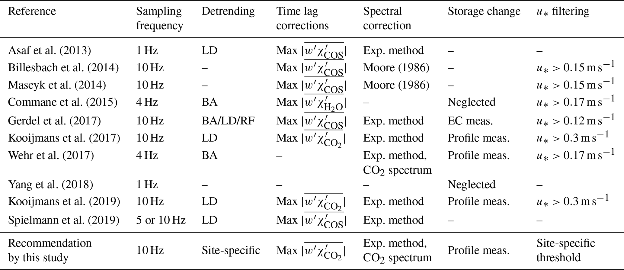
Studies on ecosystem COS flux measurements with the EC technique are still limited (Asaf et al., 2013; Billesbach et al., 2014; Maseyk et al., 2014; Commane et al., 2015; Gerdel et al., 2017; Wehr et al., 2017; Yang et al., 2018; Kooijmans et al., 2019; Spielmann et al., 2019), and there is no standardized flux processing protocol for COS EC fluxes. Table 1 summarizes the processing steps used in earlier studies. Most studies do not report all necessary steps and in particular often ignore the storage change correction. COS EC flux measurements and data processing have similarities with other trace gases (e.g., CH4 and N2O) that often have low signal-to-noise ratios, especially regarding time lag determination and frequency response corrections. Time lag determination is essential for aligning wind and gas concentration measurements to minimize biases in flux estimates. Frequency response corrections, on the other hand, are needed for correcting flux underestimation due to signal losses at both high and low frequencies (Aubinet et al., 2012). Unlike for CH4 or N2O, there are no sudden bursts or sinks expected for COS, and in that sense some processing steps for COS are more like those for CO2 (e.g., despiking, storage change correction, and friction velocity, u*, filtering). Gerdel et al. (2017) describe the issues of different detrending methods, high-frequency spectral correction, time lag determination, and u* filtering. However, there has not been any study comparing different methods for time lag determination or high-frequency spectral correction in terms of their effects on COS fluxes. This weakens our ability to assess uncertainties in COS flux measurements.
In this study, we compare different methods for detrending, time lag determination, and high-frequency spectral correction. In addition, we compare two methods for storage change flux calculation, discuss the nighttime low-turbulence problem in the context of COS EC measurements, introduce a method for gap-filling COS fluxes for the first time, and discuss the most important sources of random and systematic errors. Through the evaluation of these processing steps, we aim to settle on a set of recommended protocols for COS flux calculation.
Asaf et al. (2013)Billesbach et al. (2014)Moore (1986)Maseyk et al. (2014)Moore (1986)Commane et al. (2015)Gerdel et al. (2017)Kooijmans et al. (2017)Wehr et al. (2017)Yang et al. (2018)Kooijmans et al. (2019)Spielmann et al. (2019)Table 1Processing steps used in previous COS eddy covariance studies. Detrending methods include linear detrending (LD), block averaging (BA), and recursive filtering (RF). Spectral corrections include an experimental method and a theoretical method by Moore (1986). Processing steps not specified in the original articles are marked with a dash. The last row summarizes the recommended processing options in this study.
In this study we used COS and CO2 EC flux datasets collected at the Hyytiälä ICOS station in Finland from 26 June to 2 November 2015. The site has a long history of flux and concentration observations (Hari and Kulmala, 2005), and a COS analyzer was introduced to the site in March 2013. In this section, we describe methods used in the reference and alternative data processing schemes.
2.1 Site description
Measurements were made in a boreal Scots pine (Pinus sylvestris) stand at the Station for Measuring Forest Ecosystem–Atmosphere Relations (SMEAR II) in Hyytiälä, Finland (61∘51′ N, 24∘17′ E; 181 m above sea level). The Scots pine stand was established in 1962 and reaches at least 200 m in all directions and about 1 km to the north (Hari and Kulmala, 2005). The site is characterized by modest height variation, and an oblong lake is situated about 700 m to the southwest of the forest station (Rannik, 1998; Vesala et al., 2005). Canopy height was 17 m, and the all-sided leaf area index (LAI) was approximately 8 m2 m−2 in 2015. EC measurements were done at 23 m height. Sunrise time varied from 02:37 in June to 07:55 in November, while sunset was at 22:14 at the beginning and 16:17 at the end of the measurement period. All results are presented in Finnish winter time (UTC+2), and nighttime is defined as periods with a photosynthetic photon flux density (PPFD) of <3 µmol m−2 s−1.
2.2 EC measurement setup
The EC setup consisted of an ultrasonic anemometer (Solent Research HS1199, Gill Instruments Ltd., England, UK) for measuring wind speed in three dimensions and sonic temperature; an Aerodyne quantum cascade laser spectrometer (QCLS; Aerodyne Research Inc., Billerica, MA, USA) for measuring COS, CO2, and water vapor (H2O) mole fractions; and an LI-6262 infrared gas analyzer (LI-COR, Lincoln, NE, USA) for measuring H2O and CO2 mole fractions. All measurements were recorded at 10 Hz frequency and were made with a flow rate of approximately 10 L min−1 for the QCLS and 14 L min−1 for the LI-6262. The PTFE sampling tubes were 32 and 12 m long for QCLS and LI-6262, respectively, and both had an inner diameter of 4 mm. Two PTFE filters were used upstream of the QCLS inlet to prevent any contaminants from entering the analyzer sample cell: one coarse filter (0.45 µm, Whatman) followed by a finer filter (0.2 µm, Pall Corporation) at approximately 50 cm distance to the analyzer inlet. The Aerodyne QCLS used an electronic pressure control system to control the pressure fluctuations in the sampling cell. The QCLS was run at 20 Torr sampling cell pressure. An Edwards XDS35i scroll pump (Edwards, England, UK) was used to pump air through the sampling cell, while the LI-6262 had flow control by an LI-670 flow control unit.
Background measurements of high-purity nitrogen (N2) were done every 30 min for 26 s to remove background spectral structures in the QCLS (Kooijmans et al., 2016). In addition, a calibration cylinder was sampled each night at 00:00:45 for 15 s. The calibration cylinder consisted of COS at 429.6±5.6 ppt, CO2 at 408.37±0.05 ppm, and CO at 144.6±0.2 ppb. The cylinder was calibrated against the NOAA-2004 COS scale, WMO-X2007 CO2 scale, and WMO-X2004 CO scale using cylinders that were calibrated at the Center for Isotope Research of the University of Groningen in the Netherlands (Kooijmans et al., 2016). The standard deviation calculated from the cylinder measurements was 19 ppt for COS mixing ratios and 1.3 ppm for CO2 at 10 Hz measurement frequency.
It has previously been shown that water vapor in the sample air can affect the measurements of COS through spectral interference of the COS and H2O absorption lines (Kooijmans et al., 2016). This spectral interference was corrected for by fitting the COS spectral line separately from the H2O spectral line.
The computer embedded in the Aerodyne QCLS and the computer that controlled the sonic anemometer and logged the LI-6262 data were synchronized once a day with a separate server computer. Analog data signals from the LI-6262 were acquired by the Gill anemometer sensor input unit, which digitized the analog data and appended them to the digital output data string. Digital Aerodyne data were collected on the same computer with a serial connection and recorded in separate files with custom software (COSlog).
2.3 Profile measurements
Atmospheric concentration profiles were measured with another Aerodyne QCLS at a sampling frequency of 1 Hz. Air was sampled at five heights: 125, 23, 14, 4, and 0.5 m. A multiposition Valco valve (VICI, Valco Instruments Co. Inc.) was used to switch between the different profile heights and calibration cylinders. Each measurement height was sampled for 3 min each hour. One calibration cylinder was measured twice for 3 min each hour to correct for instrument drift, and two other calibration cylinders were measured once for 3 min each hour to assess the long-term stability of the measurements. A background spectrum was measured once every 6 h using high-purity nitrogen (N 7.0; for more details, see Kooijmans et al., 2016). The overall uncertainty of this analyzer was determined to be 7.5 ppt for COS and 0.23 ppm for CO2 at 1 Hz frequency (Kooijmans et al., 2016). The measurements are described in more detail in Kooijmans et al. (2017).
2.4 Eddy covariance fluxes
In this section, we describe the processing steps of EC flux calculation from raw data handling to final flux gap filling and uncertainties. Figure 1 provides a graphical outline of all processing steps. The different processing options presented here are applied and discussed in Sect. 3. In the next section, the different processing schemes are compared to a “reference scheme”, which consists of linear detrending, planar-fit coordinate rotation, using CO2 time lag for COS, and experimental spectral correction. A subset of the data – nighttime fluxes processed with the reference scheme – was published in Kooijmans et al. (2017).
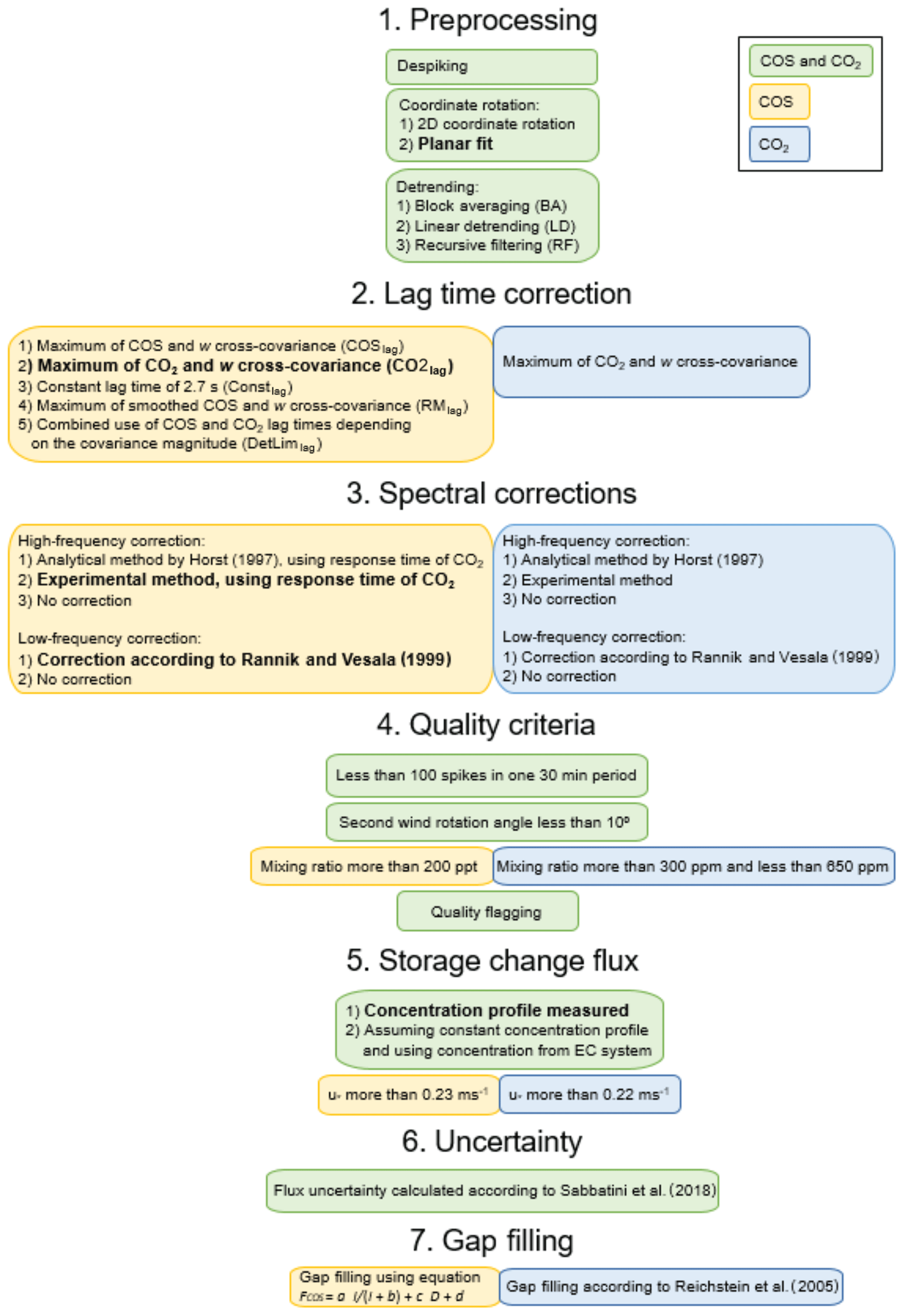
Figure 1Different EC processing steps summarized. Yellow boxes refer to steps only used for COS data processing, blue boxes to steps used only for CO2 data, and green boxes to steps that are relevant for both gases. Recommended options are written in bold. Options that are used in the reference processing scheme for COS in this study are planar-fit coordinate rotation, linear detrending, CO2 time lag, experimental high-frequency correction, low-frequency correction according to Rannik and Vesala (1999), and storage change flux from measured concentration profile. The abbreviations most commonly used throughout the text are written in parentheses.
2.4.1 Preprocessing
For flux calculation, the sonic anemometer and gas analyzer signals need to be synchronized. This is particularly relevant for fully digital systems where digital data streams are gathered from different instruments that can be completely asynchronous to each other (Fratini et al., 2018). The following procedure was used to combine two data files of 30 min length (of which one includes sonic anemometer and LI-6262 data and the other includes Aerodyne QCLS data): (1) the cross-covariance of the two CO2 signals (QCLS and LI-6262) was calculated; (2) the QCLS data were shifted so that the cross-covariance of the CO2 signals was maximized. Note that this will result in having the same time lag for the QCLS and LI-6262. The time shift between the two computers was a maximum of 10 s, with most varying between 0 and 2 s during 1 d. It is also possible to shift the time series by maximizing the covariance of CO2 and w, which will then already account for the time lag (Fig. S1 in the Supplement) or combine files according to their time stamps and allow a longer window in which the time lag is searched. However, in this case it is important that the time lag (and computer time shift) is determined from CO2 measurements only as using COS data might result in several covariance peaks in longer time frames due to low signal-to-noise ratios and small fluxes.
Raw data were then despiked so that the difference between subsequent data points was a maximum of 5 ppm for CO2, 1 mmol mol−1 for H2O, 200 ppt for COS, and 5 m s−1 for w. After despiking, the missing values were gap-filled by linear interpolation.
We used the planar-fit method to rotate the coordinate frame so that the turbulent flux divergence is as close as possible to the total flux divergence. In this method, is assumed to be zero only on longer timescales (weeks or even longer). A mean streamline plane is fitted to a long set of wind measurements. Then the z axis is fixed as perpendicular to the plane, and the wind component is fixed to be zero (Wilczak et al., 2001). In addition, we used 2D coordinate rotation for coordinate rotation in two processing schemes to determine the flux uncertainty that is related to flux data processing (Sect. 2.4.6). First, the average u component was forced to be along the prevailing wind direction. The second rotation was performed to force the mean vertical wind speed () to be zero (Kaimal and Finnigan, 1994). In this way, the x axis is parallel and z axis perpendicular to the mean flow. While 2D coordinate rotation is the most commonly used rotation method, the planar-fit method brings benefits especially in complex terrain (Lee and Finnigan, 2004) and is nowadays recommended as the preferred coordinate rotation method (Sabbatini et al., 2018).
To separate the mixing ratio time series into mean and fluctuating parts, we tested three different detrending options: (1) 30 min block averaging (BA), (2) linear detrending (LD), and (3) recursive filtering (RF) with a time constant of 30 s. BA is the most commonly used method for averaging the data with the benefit of damping the turbulent signal the least. On the other hand, BA may lead to an overestimation of the fluctuating part (and thus overestimation of the flux), for example due to instrumental drift or large-scale changes in atmospheric conditions that are not related to turbulent transfer (Aubinet et al., 2012). The LD method fits a linear regression to the averaging period and thus gets rid of instrumental drift and to some extent weather changes but may lead to underestimation of the flux if the linear trend was related to actual turbulent fluctuations in the atmosphere. The third method, RF, uses a time window (here 30 s) for a moving average over the whole averaging period. RF brings the biggest correction and thus lowest flux estimate compared to other methods but effectively removes biased low-frequency contributions to the flux. An Allan variance was determined for a time period when the instrument was sampling from a gas cylinder (Werle, 2010). The time constant of 30 s for RF was determined from the Allan plot (Fig. S4) as the system starts to drift in a nonlinear fashion at 30 s following the approach suggested by Mammarella et al. (2010). The effect of different detrending methods is shown and discussed in Sect. 3.
2.4.2 Time lag determination
The time lag between w and COS signals was determined using the following five methods:
-
The time lag was determined from the maximum difference of the cross-covariance of the COS mixing ratio and w () to a line between covariance values at the lag window limits (referred to hereafter as COSlag). This also applies to other covariance methods explained below and prevents the time lag from being exactly at the lag window limits. Lag window limits (from 1.5 to 3.8 s) were determined based on the nominal time lag of 2.6 s calculated from the flow rate and tube dimensions. More flexibility was given to the upper end of the lag window as time lags have been found to be longer than the nominal time lag (Massman, 2000; Gerdel et al., 2017).
-
The time lag was determined from the maximum difference of the cross-covariance of the CO2 mixing ratio and w () to a line between covariance values at the lag window limits within the lag window of 1.5–3.8 s (referred to hereafter as CO2lag).
-
The time lag was determined using a constant time lag of 2.6 s, which was the nominal time lag and the most common lag for CO2 with our setup (referred to hereafter as Constlag).
-
The time lag was determined from the maximum difference of the smoothed to a line between covariance values at the lag window limits. The cross-covariance was smoothed with a 1.1 s running mean (referred to hereafter as RMlag). The averaging window was chosen so that it provided a more distinguishable covariance maximum while still preventing a shift in the timing of the maximum.
-
The time lag was determined from a combination of COSlag and CO2lag. First, the random flux error due to instrument noise was calculated according to Mauder et al. (2013):
where instrumental noise was estimated from the method proposed by Lenschow et al. (2000), σw is the standard deviation of the vertical wind speed, and N is the number of data points in the averaging period. The random error was then compared to the raw maximum covariance. If the maximum covariance was higher than 3 times the random flux error, then the COSlag method was used for time lag determination. If the covariance was dominated by noise (the covariance being smaller than 3 times the random error) or COSlag was at the lag window limit, then the CO2lag lag method was selected as proposed in Nemitz et al. (2018; referred to hereafter as the DetLimlag).
2.4.3 Frequency response correction
Some of the turbulence signal is lost at both high and low frequencies due to losses in sampling lines, inadequate frequency response of the instrument, and inadequate averaging times among other reasons (Aubinet et al., 2012). In this section, we describe both high- and low-frequency loss corrections in detail. We tested two high-frequency correction methods, described below, simultaneously correcting for low-frequency losses. One run was performed with neither low-frequency nor high-frequency response corrections.
High-frequency correction
Especially in closed-path systems, the high-frequency turbulent fluctuations of the target gas damp at high frequencies due to long sampling lines. Other reasons for high-frequency losses include sensor separation and inadequate frequency response of the sensor. In turn, high-frequency losses cause the normalized cospectrum of the gas with w to be lower than expected at high frequencies, resulting in lower flux. The flux attenuation factor (FA) for a scalar s is defined as
where and are the measured and unattenuated covariances, respectively; Tws(f) is the net transfer function, specific to the EC system and scalar s; and Cows(f) is the cospectral density of the scalar flux . For solving FA, a cospectral model and transfer function are needed. In this study, we tested the effect of high-frequency spectral correction by applying either an analytical correction for high-frequency losses (Horst, 1997) or an experimental correction (Aubinet et al., 2000). The analytical correction was based on scalar cospectra defined in Horst (1997), the experimental approach was based on the assumption that temperature cospectrum is measured without significant error, and the normalized scalar cospectra were compared to the normalized temperature cospectrum (Aubinet et al., 2000; Wohlfahrt et al., 2005; Mammarella et al., 2009).
In the analytical approach by Horst (1997) the integral in Eq. (2) is solved analytically by assuming a model cospectrum of the form and a transfer function . The flux attenuation then results in
where 8 for neutral and unstable stratification, and α=1 for stable stratification in the surface layer, τs is the overall EC system time constant, and fm is the frequency of the logarithmic cospectrum peak estimated from , where nm is the normalized frequency of the cospectral peak, the mean wind speed, zm the measurement height, and d the displacement height. The normalized frequency of the cospectral peak nm is dependent on atmospheric stability (Horst, 1997):
where L is the Obukhov length (Fig. S8). The model cospectrum for the analytical high-frequency spectral correction was adapted from Kaimal et al. (1972) and given as
In the experimental approach, we solved Eq. (2) numerically and used the fitting of the measured temperature cospectra to define a site-specific scalar cospectral model (De Ligne et al., 2010) as
where the stability dependency of the cospectral peak frequency nm (Fig. S8) followed the equation
In both approaches (analytical and experimental), the time constant τs was empirically estimated by fitting the transfer function Tws(f) to the normalized ratio of cospectral densities:
where Nθ and Ns are normalization factors, and Cows and Cowθ are the scalar and temperature cospectra, respectively. The estimated time constant was 0.68 s for the Aerodyne QCLS and 0.35 s for the LI-6262.
Low-frequency correction
Detrending the turbulent time series, especially with LD or RF methods, may also remove part of the real low-frequency variations in the data (Lenschow et al., 1994; Kristensen, 1998), which should be corrected for in order to avoid flux underestimation. Low-frequency correction in this study for different detrending methods was done according to Rannik and Vesala (1999).
2.4.4 Flux quality criteria
The calculated fluxes were accepted when the following criteria were met: the second wind rotation angle (θ) was below 10∘, the number of spikes in 1 half hour was less than 100, the COS mixing ratio was higher than 200 ppt, the CO2 mixing ratio ranged between 300 and 650 ppm, and the H2O mixing ratio was higher than 1 ppb.
We used a similar flagging system for micrometeorological quality criteria as Mauder and Foken (2006) for COS and CO2: flag 0 was given if flux stationarity was less than 0.3 (meaning that covariances calculated over 5 min intervals deviate less than 30 % from the 30 min covariance), kurtosis was between 1 and 8, and skewness was within a range from −2 to 2. Flag 1 was given if flux stationarity was from 0.3 to 1 and if kurtosis and skewness were within the ranges given earlier. Flag 2 was given if these criteria were not met.
In addition to these filtering and flagging criteria, we added friction velocity (u*) filtering to screen out data collected under low-turbulence conditions. A decrease in measured EC flux is usually observed under low-turbulence conditions, although it is assumed that gas exchange should not decrease due to low turbulence. While this assumption holds for CO2, it may not be justified for COS (Kooijmans et al., 2017), as is further discussed in Sect. 3.5. The appropriate u* threshold was derived from a 99 % threshold criterion (Papale et al., 2006; Reichstein et al., 2005). The lowest acceptable u* value was determined from both COS and CO2 nighttime fluxes.
2.4.5 Storage change flux calculation
Storage change fluxes were calculated from gas mixing ratio profile measurements and by assuming a constant profile throughout the canopy using EC system mixing ratio measurements. Storage change fluxes from mixing ratio profile measurements were calculated using the formula
where p is the atmospheric pressure, Ta air temperature, R the universal gas constant, and χc(z) the gas mixing ratio at each measurement height. The integral was determined from the hourly measured χc profile at 0.5, 4, 14, and 23 m by integrating an exponential fit through the data (Kooijmans et al., 2017). When the profile measurement was not available, storage was calculated from the COS (or CO2) mixing ratio measured by the EC setup.
Another storage change flux calculation was done assuming a constant profile from the EC measurement height (23 m) to the ground level. A running average over a 5 h window was applied to the COS mixing ratio data to reduce the random noise of measurements.
The storage change fluxes were used to correct the EC fluxes for storage change of COS and CO2 below the flux measurement height.
2.4.6 Flux uncertainty
The flux uncertainty was calculated according to ICOS recommendations presented by Sabbatini et al. (2018). First, flux random error was estimated as the variance of covariance according to Finkelstein and Sims (2001):
where N is the number of data points (18 000 for 30 min of EC measurements at 10 Hz) and m the number of samples sufficiently large to capture the integral timescale (18 000 was used in this study). is the variance and the covariance of the measured variables w and c (in this case, the vertical wind velocity and gas mixing ratio).
As the chosen processing schemes affect the resulting flux, the uncertainty related to the used processing options have to be accounted for. This uncertainty was estimated as
where Fc,j is the flux calculated according to different processing schemes, and N is the number of possible processing scheme combinations that are equally reliable but cause variability in fluxes. For simplicity, the processing steps we considered here are detrending, coordinate rotation, and high-frequency spectral correction, leading to N=8 processing schemes: BA with 2D coordinate rotation and experimental spectral correction, BA with 2D rotation and Horst (1997) spectral correction, BA with planar fitting and experimental correction, BA with planar fitting and Horst (1997) correction, LD with 2D rotation and experimental correction, LD with 2D rotation and Horst (1997) correction, LD with planar fitting and experimental correction, and LD with planar fitting and Horst (1997) correction. As all the different processing schemes will lead to slightly different random errors as well, the flux random error was estimated to be the mean of Eq. (12) for different processing schemes:
The combined flux uncertainty is then the summation of ϵrand and ϵproc in quadrature:
To finally get the total uncertainty as the 95th percentile confidence interval, the total uncertainty becomes
It should be noted, though, that this uncertainty estimate holds for single 30 min fluxes only. When working with fluxes averaged over time, the total uncertainty cannot be directly propagated to the long-term averages because the two uncertainty sources behave differently. The random uncertainty is expected to decrease with increasing number of observations, while processing-related uncertainty would not be much affected by time averaging. The random uncertainty of a flux averaged over multiple observations is obtained as
where N is the number of observations and the random uncertainty of each observation (Rannik et al., 2016). In this study, we calculated the time-averaged processing uncertainty from Eq. (13) with time-averaged fluxes from the four different processing schemes. The total uncertainty of time-averaged flux was then calculated similarly from Eqs. (15) and (16) with time-averaged random and processing uncertainties.
2.4.7 Flux gap filling
Missing CO2 fluxes were gap-filled according to Reichstein et al. (2005), while missing COS fluxes were replaced by simple model estimates or by hourly mean fluxes if model estimates were not available in a way comparable to gap filling of CO2 fluxes (Reichstein et al., 2005).
The COS gap-filling function was parameterized in a moving time window of 15 d to capture the seasonality of the fluxes. To calculate gap-filled fluxes, the parameters were interpolated daily. Gaps where any driving variable of the regression model was missing were filled with the mean hourly flux during the 15 d period.
We tested different combinations of linear or saturating (rectangular hyperbola) functions of the COS flux on PPFD and linear functions of the COS flux against vapor pressure deficit (VPD) or relative humidity (RH). The saturating light response function with the mean nighttime flux as a fixed offset term explained the short-term variability of COS flux relatively well, but the residuals as a function of temperature, RH, and VPD were clearly systematic. Therefore, for the final gap filling, we used a combination of saturating function on PPFD and linear function on VPD that showed good agreement with the measured fluxes while having a relatively small number of parameters:
where I is PPFD (µmol m−2 s−1); D is VPD (kPa); and a (pmol m−2 s−1), b (µmol m−2 s−1), c (pmol m−2 s−1kPa−1), and d (pmol m−2 s−1) are fitting parameters. Parameter d was set as the median nighttime COS flux over the 15 d window, and other parameters were estimated accordingly.
3.1 Detrending methods
In order to check the contribution of different detrending methods to the resulting flux, we made flux calculations with different methods: block averaging (BA), linear detrending (LD), and recursive filtering (RF) using the same time lag (CO2 time lag) for all runs (Fig. S5).
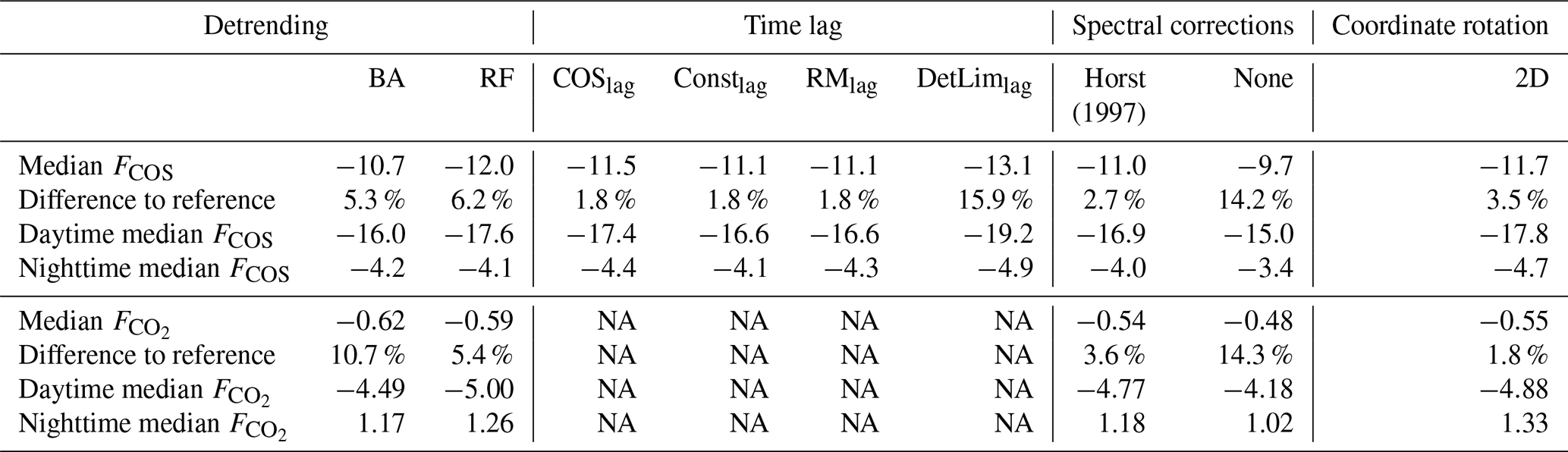
The largest median COS flux (most negative) was obtained from RF (−12.0 pmol m−2 s−1), while the smallest median (least negative) flux resulted from BA (−10.7 pmol m−2 s−1), and LD (−11.3 pmol m−2 s−1) differed by 5.3 % from BA (Table 2). The range of the 30 min COS flux was the largest (from −183.2 to 82.56 pmol m−2 s−1) when using the BA detrending method, consistent with a similar comparison in Gerdel et al. (2017). In comparison, it was from −107.3 to 73.1 pmol m−2 s−1 for LD and from −164.9 to 36.8 pmol m−2 s−1 for RF. While it was surprising that RF resulted in a more negative median flux than BA, it is likely explained by the large variation in BA with compensating high negative and positive flux values as the positive flux values with BA and LD are higher than with RF. In addition, it has to be kept in mind that the fluxes were corrected for low-frequency losses, which in part also accounts for the effects of detrending.
For CO2, the largest median flux resulted from BA (−0.62 µmol m−2 s−1). The smallest median flux resulted from LD (−0.56 µmol m−2 s−1) and RF (−0.59 µmol m−2 s−1). The difference between median CO2 flux with BA and LD was 10.7 %.
The most commonly recommended averaging methods are BA (Sabbatini et al., 2018; Nemitz et al., 2018; Moncrieff et al., 2004) and LD (Rannik and Vesala, 1999) because they have less of an impact on spectra (Rannik and Vesala, 1999) and require fewer low-frequency corrections. These are also the most used detrending methods in previous COS EC flux studies (Table 1). RF may underestimate the flux (Aubinet et al., 2012), but as spectroscopic analyzers are prone to fringe effects under field conditions, for example, the use of RF might still be justified (Mammarella et al., 2010). Regular checking of raw data provides information on instrumental drift and helps to determine the optimal detrending method. It is also recommended to check the contribution of each detrending method to the final flux to better understand what the low-frequency contribution in each measurement site and setup is.
Table 2Median COS fluxes ( pmol m−2 s−1) and CO2 fluxes ( µmol m−2 s−1) during 26 June to 2 November 2015 and their difference to the reference fluxes when using different processing options. Median reference fluxes are −11.3 pmol m−2 s−1 and −0.56 µmol m−2 s−1 for COS and CO2, respectively, and median daytime (nighttime) fluxes are −16.8 (−4.1) pmol m−2 s−1 and −4.58 (1.23) µmol m−2 s−1 when using linear detrending, CO2 time lag, and experimental high-frequency spectral correction. NA denotes that data are not available.
3.2 Effect of time lag correction
Different time lag methods resulted in slightly different time lags and COS fluxes. The most common time lags were 2.6 s from the COSlag, CO2lag, and DetLimlag methods and 1.5 s from RMlag, which was the lag window limit (Fig. 2). Time lags determined from the COSlag and RMlag methods were distributed evenly throughout the lag window, whereas the lags from the CO2lag and DetLimlag methods were normally distributed, with most lags detected at the window center.
We also tested determining time lags from the most commonly used method of maximizing the absolute covariance. If the time lag was determined from the absolute covariance maximum instead of the maximum difference to a line between covariance values at the lag window limits, the COSlag and RMlag had most values at the lag window limits (Fig. S2). This resulted in a “mirroring effect” (Langford et al., 2015); i.e., fluxes close to zero were not detected as often as with other methods since the covariance is always maximized, and the derived flux switches between positive and negative values of similar magnitude (Fig. S3). This issue should be taken into account in COS EC flux processing as absolute COS covariance maximum is by far the most commonly used method in determining the time lag in COS studies (Table 1). To make the different methods more comparable, the time lags were, in the end, determined from the maximum difference to a line between covariance values at the lag window limits in this study. In this way, time lags were not determined at the window borders, and most of the methods had the final flux probability distribution function (PDF) peak approximately at the same flux values and had otherwise small differences in the distributions (Fig. 3). The only method that was clearly different from the others was DetLimlag, which produced higher fluxes than other methods.
A constant time lag has been found to bias the flux calculation as the time lag can likely vary over time due to, for example, fluctuations in pumping speed (Langford et al., 2015; Taipale et al., 2010; Massman, 2000). However, as the CO2lag was often the same as the chosen constant lag of 2.6 s, we did not observe major differences between these two methods. A reduced bias in the flux calculation with smoothed cross-covariance was introduced by Taipale et al. (2010), who recommended using this method for any EC system with a low signal-to-noise ratio. However, we do not recommend this as a first choice since the time lags do not have a clear distribution, and if the maximum covariance method is used, we find a mirroring effect with the RMlag in the final flux distributions.
By using the DetLimlag method, the COS time lag was estimated for 54 % of cases from COSlag, while the CO2lag was used as a proxy for the COS time lag in about 46 % of cases. Figure 3 shows that the raw covariance of COS only exceeds the noise level at higher COS flux values, and thus the COSlag is chosen by this method only at higher fluxes, as expected. At lower flux rates, and especially close to zero, the COS fluxes are not high enough to surpass the noise level, and thus the CO2lag is chosen.
The median COS fluxes were highest when the time lag was determined from the DetLimlag (−13.1 pmol m−2 s−1) and COSlag (−11.5 pmol m−2 s−1) methods (Table 2). Using the COSlag results in both higher positive and negative fluxes and might thus have some compensating effect on the median fluxes. Constlag and RMlag produced the smallest median uptake (−11.1 pmol m−2 s−1), while the CO2lag had a median flux of −11.3 pmol m−2 s−1. The difference between the reference flux and the flux from the DetLimlag method was clearly higher (15.9 %) than with other methods (1.8 %) and had the largest variation (from −113.8 to 81.6 pmol m−2 s−1) and standard deviation (16.1 pmol m−2 s−1). This difference might become important at the annual scale, and as the most commonly used covariance maximization method does not produce a clear time lag distribution for DetLimlag or COSlag, we recommend using the CO2lag for COS fluxes as in most ecosystems the CO2 cross-covariance with w is more clear than the cross-covariance of COS and w signals.
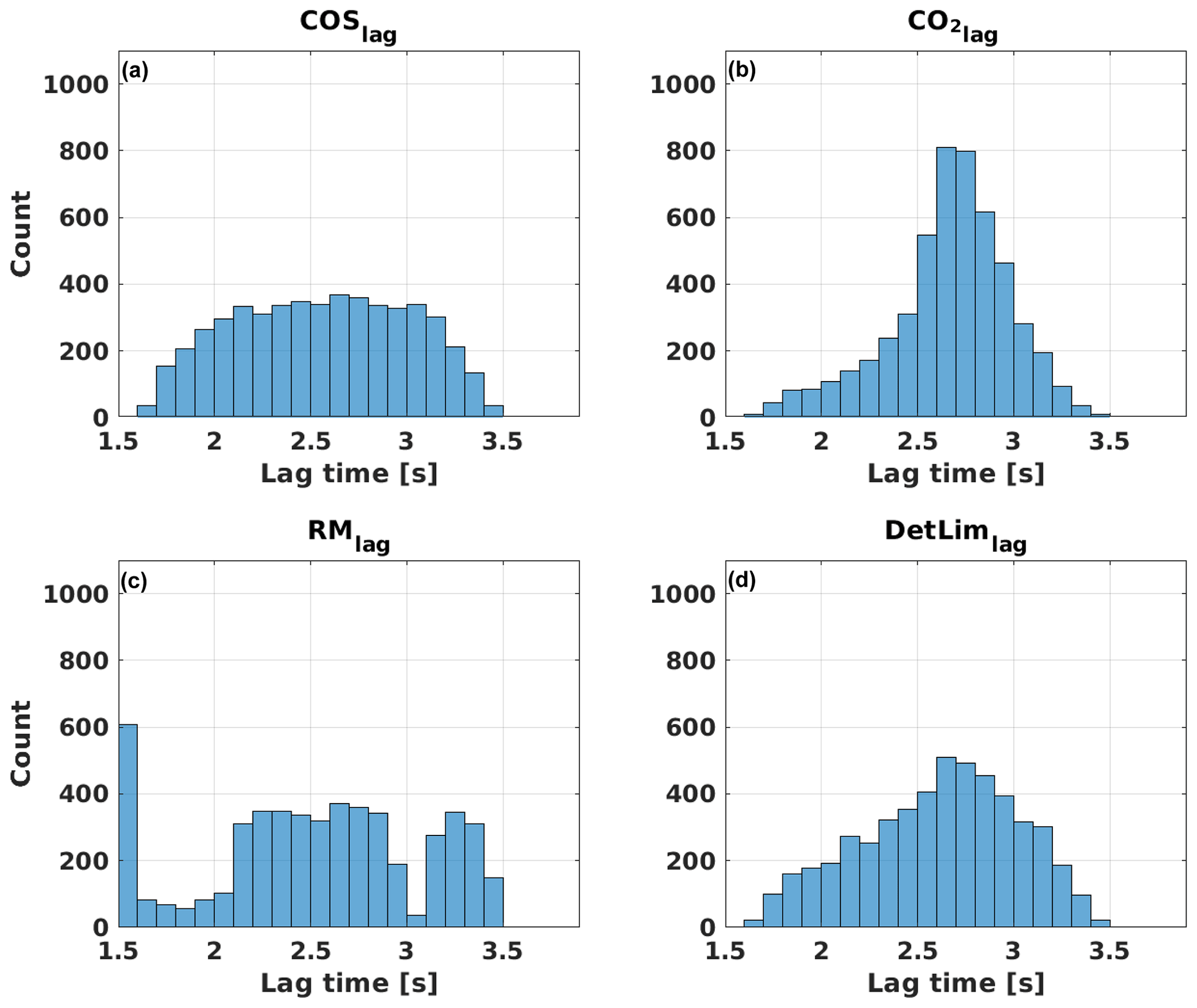
Figure 2Distribution of time lags derived from different methods: (a) COSlag, (b) CO2lag, (c) COS time lag from a running mean cross-covariance (RMlag), and (d) a combination of COSlag and CO2lag (DetLimlag).
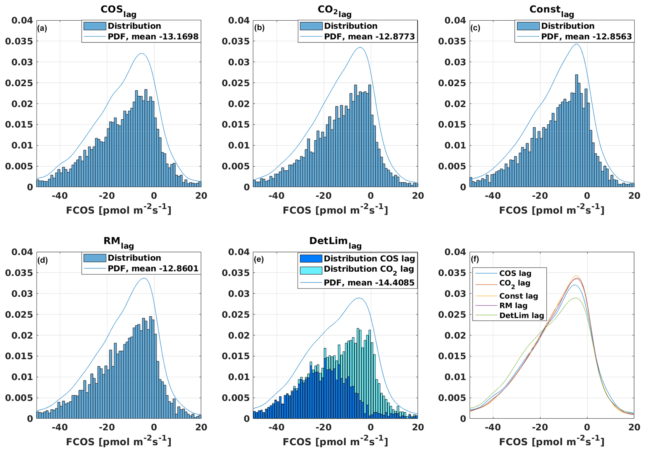
Figure 3Normalized COS flux distributions using different time lag methods: (a) COSlag, (b) CO2lag, (c) constant time lag of 2.6 s (Constlag), (d) time lag from a running mean COS cross-covariance (RMlag), (e) a combination of COS and CO2 time lags (DetLimlag), and (f) a summary of all probability distribution functions (PDFs).
3.3 High-frequency response correction
The mean COS cospectrum was close to the normal mean CO2 cospectrum (compare Fig. 4a and c). The power spectrum of COS was dominated by noise as can be seen from the increasing power spectrum with increasing frequency for normalized frequencies greater than 0.2, which is similar to what was measured for COS by Gerdel et al. (2017) and for N2O by Eugster et al. (2007). The fact that COS measurements are dominated by noise at high frequencies means that those measurements are limited by precision and that they likely do not capture the true variability in COS turbulence signals. This is less of a problem for CO2, where white noise only starts to dominate at higher frequencies (normalized frequency higher than 3). Cospectral attenuation was found for both COS and CO2 at high frequency.
High-frequency losses due to, for example, attenuation in sampling tubes and limited sensor response times are expected to decrease fluxes if not corrected for (Aubinet et al., 2012). The median COS flux, when using the CO2 time lag and keeping low-frequency correction and quality filtering the same, was the least negative without any high-frequency correction (−9.7 pmol m−2 s−1), most negative with the experimental correction (−11.3 pmol m−2 s−1), and in between with the analytical correction (−11.0 pmol m−2 s−1; Fig. S6). Correcting for the high-frequency attenuation thus made a maximum of 14.2 % difference in the median COS flux. In addition, daytime median flux magnitudes increased from −15.0 to −16.9 pmol m−2 s−1 with the analytical correction and to −16.8 pmol m−2 s−1 with the experimental high-frequency correction. However, the relative difference was larger during nighttime, when flux magnitudes increased from −3.4 to −4.0 and −4.1 pmol m−2 s−1 with analytical and experimental methods, respectively.
Similar results were found for the CO2 flux, but the differences were smaller: without any high-frequency correction the median flux was the least negative at −0.48 µmol m−2 s−1, most negative with experimental correction (−0.56 µmol m−2 s−1), and in between with the analytical correction (−0.54 µmol m−2 s−1), thus making a maximum of 14.3 % difference in the median CO2 flux, similar to COS. Very similar results were found for CH4 and CO2 fluxes in Mammarella et al. (2016), where the high-frequency correction made the largest difference in the final flux processing for closed-path analyzers. Similar to COS, CO2 flux magnitudes were also increased more during nighttime due to spectral correction than during daytime. Daytime median flux magnitude increased from −4.18 to −4.77 and −4.58 µmol m−2 s−1, and nighttime fluxes increased from 1.02 to 1.18 and 1.23 µmol m−2 s−1 when using analytical and experimental high-frequency spectral corrections, respectively. Flux attenuation was dependent on stability and wind speed for both correction methods, as also found in Mammarella et al. (2009; Fig. S7).
The site-specific model captures the cospectrum better than the model cospectrum by Horst (1997), as shown in Fig. 4. For high-frequency spectral corrections, it is recommended to use the site-specific cospectral model, as has been done in most previous COS studies (Table 1).
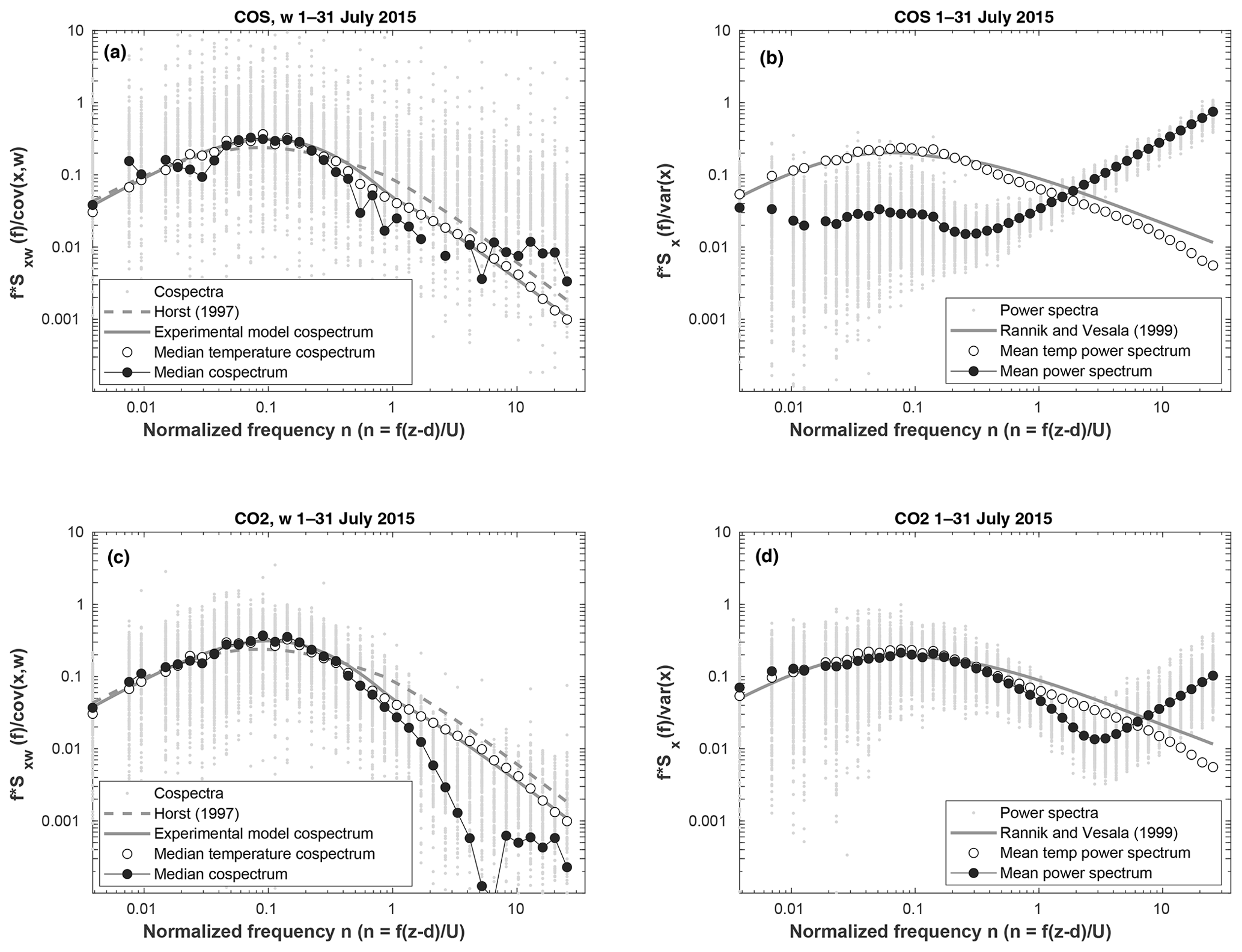
Figure 4Cospectrum and power spectrum for COS (panels a and b, respectively) and CO2 (panels c and d, respectively) in July 2015. All data were filtered by the stability condition , and COS data were only accepted when the covariance was higher than 3 times the random error due to instrument noise (Eq. 1). The cospectrum models by the experimental method and Horst (1997) that were used in the high-frequency spectral correction are shown in continuous and dashed gray lines, respectively.
3.4 Storage change fluxes
In the following, storage change fluxes based on profile measurements are listed as default, with fluxes based on the constant profile assumption listed in brackets.
The COS storage change flux was negative from 15:00 until 06:00, with a minimum of −1.0 pmol m−2 s−1 (−0.6 pmol m−2 s−1) reached at 20:00. A negative storage change flux of COS indicates that there is a COS sink in the ecosystem when the boundary layer and effective mixing layer is shallow. Neglecting this effect would lead to overestimated uptake at the ecosystem level later when the air at the EC sampling height is better mixed. The COS storage change flux was positive from around 06:00 until 15:00 and peaked at 09:00 with a magnitude of 1.9 pmol m−2 s−1 (0.8 pmol m−2 s−1). The storage change flux made the highest relative contribution to the sum of measured EC and storage change fluxes at midnight with 18 % (13 %; Fig. 5c). The difference between the two methods was a minimum of 13 % at 11:00 and a maximum of 56 % at 09:00. The two methods made a maximum of 7 % difference in the resulting cumulative ecosystem flux, as already reported in Kooijmans et al. (2017).
The CO2 storage change flux was positive from 15:00 until around 04:00, with a maximum value of 0.62 µmol m−2 s−1 (0.38 µmol m−2 s−1) reached at 21:00. A positive storage change flux indicates that the ecosystem contains a source of carbon when the boundary layer is less turbulent and accumulates the respired CO2 within the canopy. As turbulence would increase later in the morning, the accumulated CO2 would result in an additional flux that could mask the gas exchange processes occurring at that time step. The CO2 storage change flux minimum was reached with both methods at 08:00, with a magnitude of −1.01 µmol m−2 s−1 (−0.52 µmol m−2 s−1) when the boundary layer had already started expanding, and leaves are assimilating CO2. The maximum contribution of the storage change flux was as high as 89 % (36 %) compared to the EC flux at 18:00, when the CO2 exchange turned to respiration, and storage change flux increased its relative importance (Fig. 5d). The difference between the two storage change flux methods for CO2 was a maximum of 53 % at 21:00 and a minimum of 13 % at midnight. The maximum difference of 5 % was found in the cumulative ecosystem CO2 flux when the different methods were used.
In conclusion, the storage change fluxes are not relevant for budget calculations, as expected, and have not been widely applied in previous COS studies (Table 1) even though storage change flux measurements are mandatory in places where the EC system is placed at a height of 4 m or above according to the ICOS protocol for EC flux measurements (Montagnani et al., 2018). In addition, storage change fluxes are important at the diurnal scale to account for the delayed capture of fluxes by the EC system under low-turbulence conditions.
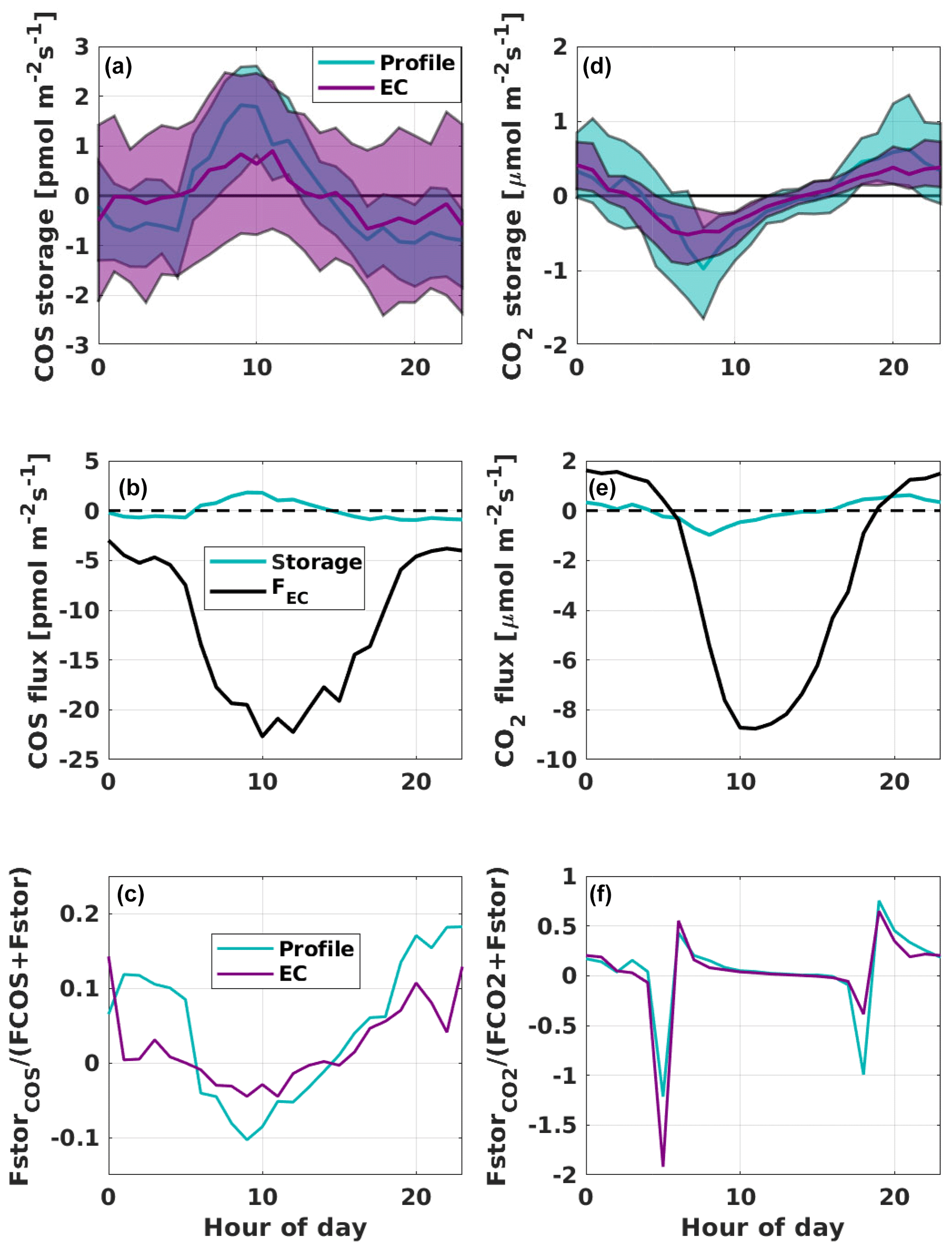
Figure 5Diurnal variation in the storage change flux, determined from (a) COS and (d) CO2 profile measurements (blue) and by assuming a constant profile up to 23 m height (purple), and diurnal variation in the EC flux (black) and storage change flux with the profile method (blue; panels b and e for COS and CO2 fluxes, respectively) during the measurement period 26 June to 2 November 2015. Contribution of storage change flux to the total ecosystem EC flux with the profile measurements and assuming a constant profile for (c) COS and (f) CO2.
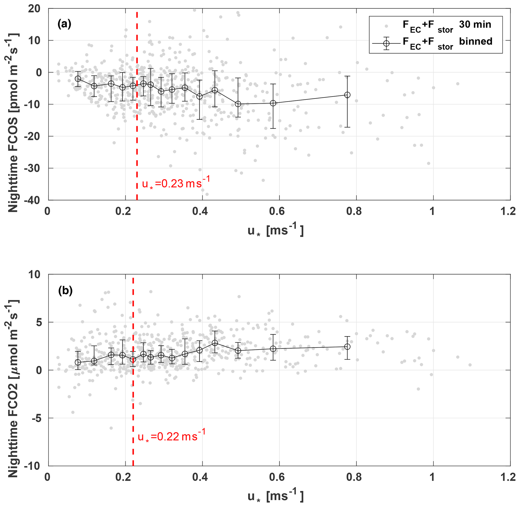
Figure 6Nighttime median ecosystem fluxes (black) of (a) COS and (b) CO2 binned into 15 equal-sized friction velocity bins. Error bars indicate ranges between the 25th and 75th percentiles. Friction velocity thresholds are shown with dashed red lines and single data points of 30 min fluxes with light gray dots.
3.5 u* filtering
Calm and low-turbulence conditions are especially common during nights with stable atmospheric stratification. In this case, storage change and advective fluxes have an important role, and the measured EC flux of a gas does not reflect the atmosphere–biosphere exchange, typically underestimating the exchange. This often leads to a systematic bias in the annual flux budgets (Moncrieff et al., 1996; Aubinet et al., 2000; Aubinet, 2008). Even after studies of horizontal and vertical advection, u* filtering still keeps its place as the most efficient and reliable tool to filter out data that are not representative of the surface–atmosphere exchange under low turbulence (Aubinet et al., 2010).
For COS, nighttime filtering is a more complex issue than it is for CO2. In contrast to CO2, COS is taken up by the ecosystem during nighttime (Kooijmans et al., 2017, 2019) depending on stomatal conductance and the concentration gradient between the leaf and the atmosphere. When the atmospheric COS mixing ratio decreases under low-turbulence conditions (due to nighttime COS uptake in the ecosystem), the concentration gradient between the leaf and the atmosphere goes down such that a decrease in COS uptake can be expected (Kooijmans et al., 2017). Thus, the assumption that fluxes do not go down under low-turbulence conditions, as is the case for respiration of CO2, does not necessarily apply to COS uptake. Gap-filling the u*-filtered COS fluxes may therefore create a bias due to false assumptions if the gap filling is only based on data from periods with high turbulence. However, as we did not see u* dependency disappearing even with a concentration-gradient-normalized flux, the u* filtering and proceeding gap filling were applied here as usual (Papale et al., 2006) to overcome the EC measurement limitations under low-turbulence conditions.
We determined u* limits of 0.23 m s−1 for COS and 0.22 m s−1 for CO2 (Fig. 6). Filtering according to these u* values would remove 12 % and 11 % of data, respectively. If the storage change flux was excluded when determining the u* threshold, the limits were 0.39 and 0.24 m s−1 from CO2 and COS fluxes, respectively. The increase in the u* threshold with CO2 is because the fractional storage change flux is larger for CO2 than for COS (Fig. 5c and f). On the other hand, the u* limit for COS stayed similar to the previous one. With these u* thresholds the filtering would exclude 30 % and 13 % of the data for COS and CO2 respectively.
If fluxes are not corrected for storage before deriving the u* threshold, there is a risk of flux overestimation due to double accounting. The flux data filtered for low turbulence would be gap-filled, thereby accounting for storage by the canopy, but then accounted for again when the storage is released and measured by the EC system during the flushing hours in the morning (Papale et al., 2006). Thus, it is necessary to make the storage change flux correction before deriving u* thresholds and applying the filtering.
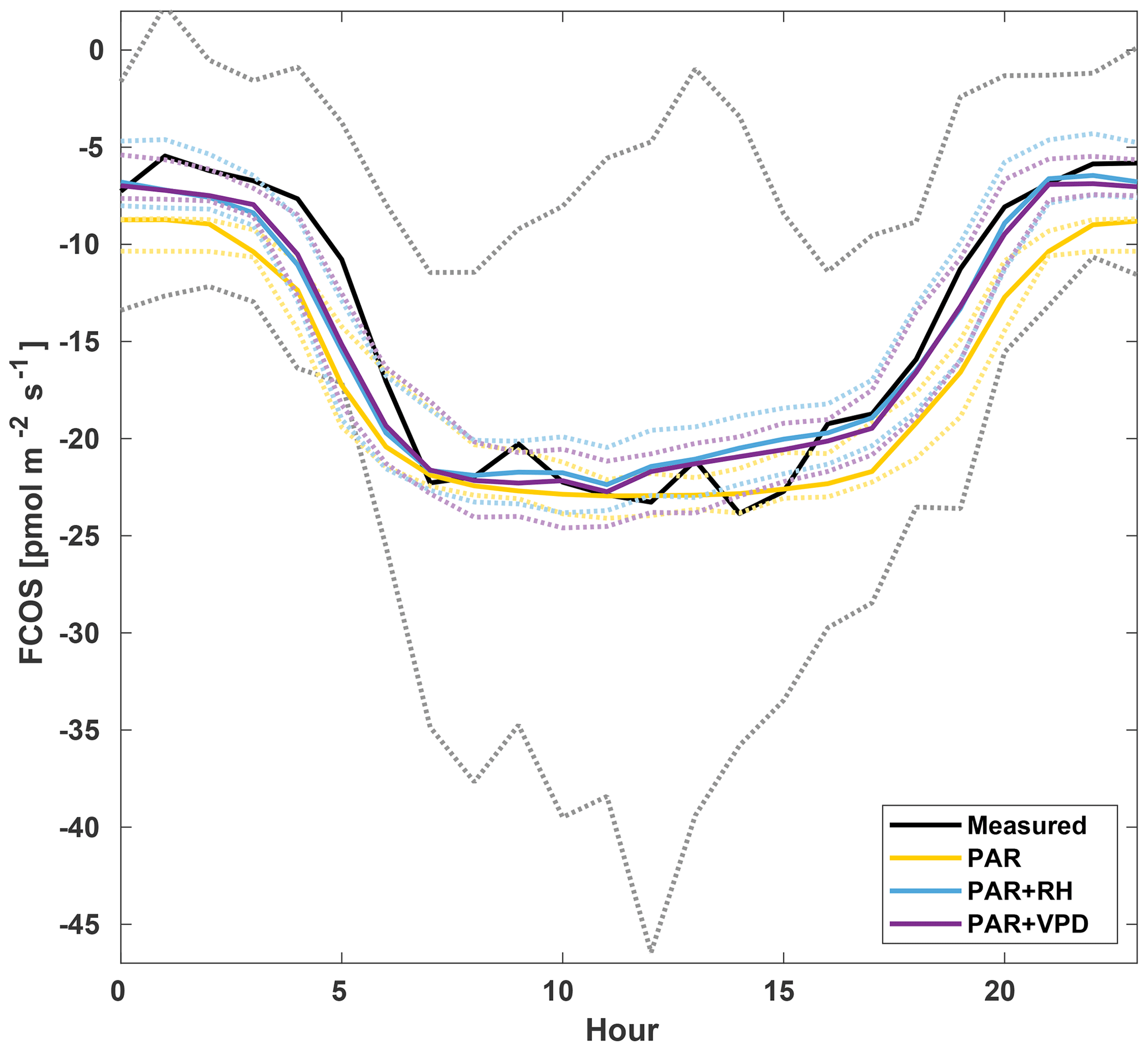
Figure 7Diurnal variation in the measured COS flux (black) and the flux from different gap-filling methods: gap filling with only saturating PAR function (yellow), saturating PAR and linear dependency on RH (blue), and saturating PAR and linear dependency on VPD (purple). Diurnal variation is calculated from 1 July to 31 August 2015 for periods when measured COS flux existed. Dashed lines represent the 25th and 75th percentiles.
3.6 Gap filling
Three combinations of environmental variables (PAR, PAR and RH, and PAR and VPD) were tested using the gap-filling function (Eq. 18). These environmental parameters were chosen because COS exchange has been found to depend on stomatal conductance, which in turn depends especially on radiation and humidity (Kooijmans et al., 2019). Development of the gap-filling parameters a, b, c, and d over the measurement period is presented in Fig. S10. While the saturating function of PAR alone already captured the diurnal variation relatively well, adding a linear dependency on VPD or RH made the diurnal pattern even closer to the measured one, although some deviation is still observed, especially in the early morning (Fig. 7). Therefore, the combination of saturating light response curve and linear VPD dependency was chosen. Furthermore, we chose a linear VPD dependency instead of a linear RH dependency due to smaller residuals in the former (Fig. S9). The mean residual of the chosen model was −0.54 pmol m−2 s−1, and the root mean square error (RMSE) was 18.7 pmol m−2 s−1, while the saturating PAR function with linear RH dependency had a mean residual of −0.84 and an RMSE of 19.3 pmol m−2 s−1, and the saturating PAR function had a residual of 0.97 pmol m−2 s−1 and an RMSE of 22.8 pmol m−2 s−1.
For COS fluxes, 44 % of daytime flux measurements were discarded due to the above-mentioned quality criteria (Sect. 2.4.4) and low-turbulence filtering. As expected, more data (66 %) were discarded during nighttime. Altogether, 52 % of all COS flux data were discarded and gap-filled with the gap-filling function presented in Eq. (18). The average of the corrected and gap-filled COS fluxes during the whole measurement period was −12.3 pmol m−2 s−1, while without gap filling the mean flux was 14 % more negative, −14.3 pmol m−2 s−1. This indicates that most gap filling was done for the nighttime data, when COS fluxes are less negative than during daytime.
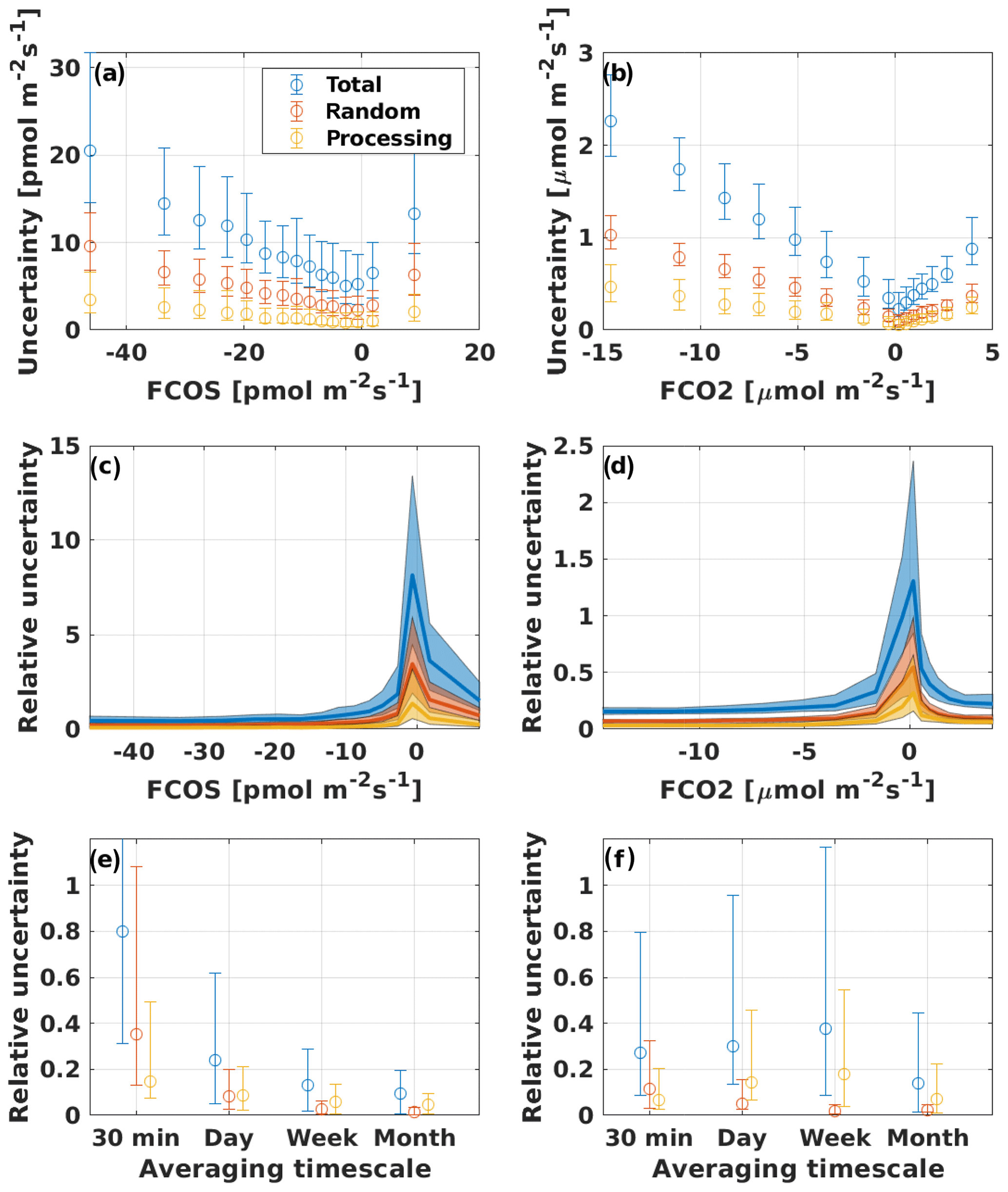
Figure 8Uncertainty of (a) COS and (b) CO2 fluxes, binned into 15 equal-sized bins that represent median values. Error bars show the 25th and 75th percentiles. Total uncertainty is represented as the 95 % confidence interval (1.96ϵcomb). Panels (c) and (d) represent the relative uncertainty, i.e., the uncertainty divided by the flux for COS and CO2, respectively. Panels (e) and (f) represent the relative uncertainties of time-averaged COS and CO2 fluxes, respectively.
For CO2, 41 % of daytime CO2 fluxes were discarded, while 67 % of fluxes were discarded during nighttime, altogether comprising 53 % of all CO2 flux data. CO2 fluxes were gap-filled according to standard gap-filling procedures presented in Reichstein et al. (2005). The average CO2 flux after all corrections and gap filling was −2.14 µmol m−2 s−1, while without gap filling the mean flux was 39 % more negative, −3.53 µmol m−2 s−1. Similar to COS, CO2 fluxes are also mostly gap-filled during nighttime. As nighttime CO2 fluxes are positive, gap-filled fluxes include more positive values than non-gap-filled fluxes, thus making the mean flux less negative.
Although the COS community has not been interested in the cumulative COS fluxes or yearly COS budget so far, it is important to fill short-term gaps in COS flux data to properly capture the diurnal variation, for example. The gap-filling method presented here is one option to be tested at other measurement sites as well.
3.7 Errors and uncertainties
The uncertainty due to the chosen processing scheme was determined from a combination of eight different processing schemes, as described in Sect. 2.4.6, that were equally reliable but caused the most variation in the final COS flux (Table 2). This processing uncertainty contributed 36 % to the total uncertainty of the 30 min COS flux, while the rest was composed of the random flux uncertainty (Fig. 8). For the CO2 flux uncertainty, the processing was more important than for COS (48 %), but the random uncertainty still dominated the combined flux uncertainty. The random error of the CO2 flux was found to be lower than in Rannik et al. (2016) for the same site, probably related to differences in the gas analyzers and overall setup. The mean noise estimated from Lenschow et al. (2000) was 0.06 µmol m−2 s−1 for our QCLS CO2 fluxes, while in Rannik et al. (2016) it was approximately 0.08 µmol m−2 s−1 for LI-6262 CO2 fluxes at the same site. Gerdel et al. (2017) found the total random uncertainty of COS fluxes to be mostly around 3–8 pmol m−2 s−1, comparable to our results.
The relative flux uncertainty for COS was very high at low flux (−3 pmol m−2 s pmol m−2 s−1) values (8 times the actual flux value) but leveled off to 45 % at fluxes higher (meaning more negative fluxes) than −27 pmol m−2 s−1 (Fig. 8c). The total uncertainty of the CO2 flux was also high at low fluxes (−1.5 µmol m−2 s µmol m−2 s−1, uncertainty reaching 130 % of the flux at 0.17 µmol m−2 s−1) and decreased to 15 % at fluxes more negative than −11 µmol m−2 s−1 (Fig. 8d). Higher relative uncertainty at low flux levels is probably due to the detection limit of the measurement system.
The median relative random uncertainty of COS flux decreased from 0.35 for single 30 min flux to 0.013 for monthly averaged flux (Fig. 8e). The processing uncertainty had a less prominent decrease, from 0.15 for 30 min fluxes to 0.05 for monthly fluxes. The strongest decrease in processing uncertainty was when moving from single 30 min flux values to daily average fluxes, after which the averaging period did not affect the processing uncertainty. This is probably due to the large scatter between the two detrending methods, which levels off when averaging over several flux values (Fig. S11a). Relative random uncertainty of CO2 flux decreased from 0.11 for 30 min fluxes to 0.021 for monthly fluxes. The processing uncertainty, however, did not change significantly between the different averaging periods, as would be expected.
In this study, we examined the effects of different processing steps on COS EC fluxes and compared them to CO2 flux processing. COS fluxes were calculated with five time lag determination methods, three detrending methods, two high-frequency spectral correction methods, and with no spectral corrections. We calculated the storage change fluxes of COS and CO2 from two different concentration profiles and investigated the diurnal variation in the storage change fluxes. We applied u* filtering and introduced a gap-filling method for COS fluxes. We also quantified the uncertainties of COS and CO2 fluxes.
The largest differences in the final fluxes came from time lag determination and detrending. Different time lag methods made a difference of a maximum of 15.9 % in the median COS flux. Different detrending methods, on the other hand, made a maximum of 6.2 % difference in the median COS flux, while it was more important for CO2 (10.7 % difference between linear detrending and block averaging). Omitting high-frequency spectral correction resulted in a 14.2 % lower median flux, while different methods used in high-frequency spectral correction resulted in only 2.7 % difference in the final median fluxes. We suggest using CO2 time lag for COS flux calculation so that potential biases due to a low signal-to-noise ratio of COS mixing ratio measurements can be eliminated. The CO2 mixing ratio is measured simultaneously with the COS mixing ratio with the Aerodyne QCLS, and in most cases it has a higher signal-to-noise ratio and more clear cross-covariance with w than COS. Experimental high-frequency correction is recommended for accurately correcting for site-specific spectral losses. We recommend comparing the effect of different detrending methods on the final flux for each site separately to determine the site- and instrument-specific trends in the raw data.
Flux uncertainties of COS and CO2 followed a similar trend of higher relative uncertainty at low flux values and random flux uncertainty dominating over uncertainty related to processing in the total flux uncertainty. The relative uncertainty was more than 5 times higher for COS than for CO2 at low flux values (absolute COS flux of less than 3 pmol m−2 s−1), while at higher fluxes they were more similar. When averaging fluxes over time, the relative random uncertainty decreased with increasing averaging period for both COS and CO2. Relative processing uncertainty decreased from single 30 min COS fluxes to daily averages but remained at the same level for longer averaging periods.
We emphasize the importance of time lag method selection for small fluxes, whose uncertainty may exceed the flux itself, to avoid systematic biases. COS EC flux processing follows similar steps as other fluxes with low signal-to-noise ratios, such as CH4 and N2O, but as there are no sudden bursts of COS expected, and its diurnal behavior is close to CO2, some processing steps are more similar to CO2 flux processing. In particular, time lag determination and high-frequency spectral corrections should follow the protocol of low signal-to-noise ratio fluxes (Nemitz et al., 2018), while quality assurance and quality control, despiking, u* filtering, and storage change correction should follow the protocol produced for CO2 flux measurements (Sabbatini et al., 2018). Our recommendation for time lag determination (CO2 cross-covariance) differs from the most commonly used method so far (COS cross-covariance), while experimental high-frequency spectral correction has already been widely applied before (Table 1). Many earlier studies have neglected the storage change flux, but we emphasize its importance in the diurnal variation in COS exchange. In addition, we encourage implementing gap filling in future COS flux calculations for eliminating short-term gaps in data.
The flux data used in this study are available in Kohonen (2020; https://doi.org/10.5281/zenodo.3907342). Environmental data are available on the AVAA open research data publishing platform (https://avaa.tdata.fi/web/smart/smear/download, last access: 17 March 2020; Junninen et al. , 2009). The metadata of the environmental observations are available via the ETSIN service. Raw data and flux data processed with different schemes other than the standard scheme are available upon request from the first author.
The supplement related to this article is available online at: https://doi.org/10.5194/amt-13-3957-2020-supplement.
K-MK and IM designed the study, and K-MK processed and analyzed the data. PK developed the gap-filling function for COS and participated in data processing. IM, LMJK, US, WS, and HC participated in field measurements. K-MK and IM wrote the manuscript, with major participation in editing by WS and LMJK and contributions from all coauthors.
The authors declare that they have no conflict of interest.
We thank the Hyytiälä Forestry Field Station staff for all their technical support, especially Helmi-Marja Keskinen and Janne Levula. Kukka-Maaria Kohonen thanks the Vilho, Yrjö and Kalle Väisälä foundation for its kind support.
This research has been supported by the ICOS Finland (grant no. 319871), the Academy of Finland Center of Excellence (grant no. 307331), the Academy of Finland Academy Professor project (grant no. 284701), and the ERC Advanced funding scheme (abbreviation: COS-OCS; grant no. 742798).
Open-access funding provided by Helsinki University Library.
This paper was edited by Christof Ammann and reviewed by Georg Wohlfahrt and two anonymous referees.
Asaf, D., Rotenberg, E., Tatarinov, F., Dicken, U., Montzka, S. A., and Yakir, D.: Ecosystem photosynthesis inferred from measurements of carbonyl sulphide flux, Nat. Geosci., 6, 186–190, https://doi.org/10.1038/NGEO1730, 2013. a, b, c, d
Aubinet, M.: Eddy covariance CO2 flux measurements in nocturnal conditions: an analysis of the problem, Ecol. Appl., 18, 1368–1378, 2008. a
Aubinet, M., Grelle, A., Ibrom, A., Rannik, Ü., Moncrieff, J., Foken, T., Kowalski, A. S., Martin, P. H., Berbigier, P., Bernhofer, C., Clement, R., Elbers, J., Granier, A., Grünwald, T., Morgenstern, K., Pilegaard, K., Rebmann, C., Snijders, W., Valentini, R., and Vesala, T.: Estimates of the annual net carbon and water exchange of forests: the EUROFLUX methodology, in: Advances in ecological research, 30, 113–175, 2000. a, b, c
Aubinet, M., Feigenwinter, C., Heinesch, B., Bernhofer, C., Canepa, E., Lindroth, A., Montagnani, L., Rebmann, C., Sedlak, P., and Van Gorsel, E.: Direct advection measurements do not help to solve the night-time CO2 closure problem: Evidence from three different forests, Agr. Forest Meteorol., 150, 655–664, 2010. a
Aubinet, M., Vesala, T., and Papale (Eds.), D.: Eddy covariance: a practical guide to measurement and data analysis, Springer Science & Business Media, 2012. a, b, c, d, e, f
Billesbach, D., Berry, J., Seibt, U., Maseyk, K., Torn, M., Fischer, M., Abu-Naser, M., and Campbell, J.: Growing season eddy covariance measurements of carbonyl sulfide and CO2 fluxes: COS and CO2 relationships in Southern Great Plains winter wheat, Agr. Forest Meteorol., 184, 48–55, https://doi.org/10.1016/j.agrformet.2013.06.007, 2014. a, b
Blonquist, J. M., Montzka, S. A., Munger, J. W., Yakir, D., Desai, A. R., Dragoni, D., Griffis, T. J., Monson, R. K., Scott, R. L., and Bowling, D. R.: The potential of carbonyl sulfide as a proxy for gross primary production at flux tower sites, J. Geophys. Res., 116, G04019, https://doi.org/10.1029/2011JG001723, 2011. a
Commane, R., Meredith, L., Baker, I. T., Berry, J. A., Munger, J. W., and Montzka, S. A.: Seasonal fluxes of carbonyl sulfide in a midlatitude forest, P. Natl. Acad. Sci. USA, 112, 14162–14167, https://doi.org/10.1073/pnas.1504131112, 2015. a, b
De Ligne, A., Heinesch, B., and Aubinet, M.: New transfer functions for correcting turbulent water vapour fluxes, Bound.-Lay. Meteorol., 137, 205–221, 2010. a
Eugster, W., Zeyer, K., Zeeman, M., Michna, P., Zingg, A., Buchmann, N., and Emmenegger, L.: Methodical study of nitrous oxide eddy covariance measurements using quantum cascade laser spectrometery over a Swiss forest, Biogeosciences, 4, 927–939, https://doi.org/10.5194/bg-4-927-2007, 2007. a
Finkelstein, P. and Sims, P.: Sampling error in eddy correlation flux measurements, J. Geophys. Res.-Atmos., 106, 3503–3509, 2001. a
Franz, D., Acosta, M., Altimir, N. et al.: Towards long-term standardized carbon and greenhouse gas observations for monitoring Europe’s terrestrial ecosystems: a review, Int. Agrophys., 32, 471–494, https://doi.org/10.1515/intag-2017-0039, 2018. a
Fratini, G., Sabbatini, S., Ediger, K., Riensche, B., Burba, G., Nicolini, G., Vitale, D., and Papale, D.: Eddy covariance flux errors due to random and systematic timing errors during data acquisition, Biogeosciences, 15, 5473–5487, https://doi.org/10.5194/bg-15-5473-2018, 2018. a
Gerdel, K., Spielmann, F. M., Hammerle, A., and Wohlfahrt, G.: Eddy covariance carbonyl sulfide flux measurements with a quantum cascade laser absorption spectrometer, Atmos. Meas. Tech., 10, 3525–3537, https://doi.org/10.5194/amt-10-3525-2017, 2017. a, b, c, d, e, f, g
Hari, P. and Kulmala, M.: Station for Measuring Ecosystem–Atmosphere Relations (SMEAR II), Boreal Environ. Res., 10, 315–322, 2005. a, b
Horst, T. W.: A Simple Formula for Attenuation of Eddy Fluxes, Bound.-Lay. Meteorol., 82, 219–233, 1997. a, b, c, d, e, f, g, h, i, j
Junninen, H., Lauri, A., Keronen, P., Aalto, P., Hiltunen, V., Hari, P., and Kulmala, M.: Smart-SMEAR: on-line data exploration and visualization tool for SMEAR stations, Boreal Environ. Res., 14, 447–457, 2009. a
Kaimal, J., Wyngaard, J., Izumi, Y., and Coté, O.: Spectral characteristics of surface-layer turbulence, Q. J. Roy. Meteor. Soc., 98, 563–589, 1972. a
Kaimal, J. C. and Finnigan, J. J.: Atmospheric boundary layer flows: their structure and measurement, Oxford university press, 1994. a
Kohonen, K.-M.: Data for “Towards standardized processing of eddy covariance flux measurements of carbonyl sulfide”, Zenodo, https://doi.org/10.5281/zenodo.3907342, 2020.
Kooijmans, L. M., Sun, W., Aalto, J., Erkkilä, K.-M., Maseyk, K., Seibt, U., Vesala, T., Mammarella, I., and Chen, H.: Influences of light and humidity on carbonyl sulfide-based estimates of photosynthesis, P. Natl. Acad. Sci. USA, 116, 2470–2475, 2019. a, b, c, d, e
Kooijmans, L. M. J., Uitslag, N. A. M., Zahniser, M. S., Nelson, D. D., Montzka, S. A., and Chen, H.: Continuous and high-precision atmospheric concentration measurements of COS, CO2, CO and H2O using a quantum cascade laser spectrometer (QCLS), Atmos. Meas. Tech., 9, 5293–5314, https://doi.org/10.5194/amt-9-5293-2016, 2016. a, b, c, d, e
Kooijmans, L. M. J., Maseyk, K., Seibt, U., Sun, W., Vesala, T., Mammarella, I., Kolari, P., Aalto, J., Franchin, A., Vecchi, R., Valli, G., and Chen, H.: Canopy uptake dominates nighttime carbonyl sulfide fluxes in a boreal forest, Atmos. Chem. Phys., 17, 11453–11465, https://doi.org/10.5194/acp-17-11453-2017, 2017. a, b, c, d, e, f, g, h
Kristensen, L.: Time series analysis, Dealing with imperfect data, Riso National Laboratory, Roskilde, Denmark, 1998. a
Langford, B., Acton, W., Ammann, C., Valach, A., and Nemitz, E.: Eddy-covariance data with low signal-to-noise ratio: time-lag determination, uncertainties and limit of detection, Atmos. Meas. Tech., 8, 4197–4213, https://doi.org/10.5194/amt-8-4197-2015, 2015. a, b
Lee, X. and Finnigan, J.: Coordinate systems and flux bias error, in: Handbook of Micrometeorology, 33–66, Springer, 2004. a
Lenschow, D., Mann, J., and Kristensen, L.: How long is long enough when measuring fluxes and other turbulence statistics?, J. Atmos. Ocean. Tech., 11, 661–673, 1994. a
Lenschow, D., Wulfmeyer, V., and Senff, C.: Measuring Second- through Fourth-Order Moments in Noisy Data, J. Atmos. Ocean. Tech., 17, 1330–1347, 2000. a, b
Mammarella, I., Launiainen, S., Grönholm, T., Keronen, P., Pumpanen, J., Rannik, Ü., and Vesala, T.: Relative humidity effect on the high-frequency attenuation of water vapor flux measured by a closed-path eddy covariance system, J. Atmos. Ocean. Tech., 26, 1856–1866, https://doi.org/10.1175/2009JTECHA1179.1, 2009. a
Mammarella, I., Werle, P., Pihlatie, M., Eugster, W., Haapanala, S., Kiese, R., Markkanen, T., Rannik, Ü., and Vesala, T.: A case study of eddy covariance flux of N2O measured within forest ecosystems: quality control and flux error analysis, Biogeosciences, 7, 427–440, https://doi.org/10.5194/bg-7-427-2010, 2010. a, b
Mammarella, I., Peltola, O., Nordbo, A., Järvi, L., and Rannik, Ü.: Quantifying the uncertainty of eddy covariance fluxes due to the use of different software packages and combinations of processing steps in two contrasting ecosystems, Atmos. Meas. Tech., 9, 4915–4933, https://doi.org/10.5194/amt-9-4915-2016, 2016. a
Maseyk, K., Berry, J. A., Billesbach, D., Campbell, J. E., Torn, M. S., Zahniser, M., and Seibt, U.: Sources and sinks of carbonyl sulfide in an agricultural field in the Southern Great Plains, P. Natl. Acad. Sci. USA, 111, 9064–9069, https://doi.org/10.1073/pnas.1319132111, 2014. a, b
Massman, W. J.: A simple method for estimating frequency response corrections for eddy covariance systems, Agr. Forest Meteorol., 104, 185–198, 2000. a, b
Mauder, M. and Foken, T.: Impact of post-field data processing on eddy covariance flux estimates and energy balance closure, Meteorol. Z., 15, 597–609, 2006. a
Mauder, M., Cuntz, M., Drüe, C., Graf, A., Rebmann, C., Peter, H., Schmidt, M., and Steinbrecher, R.: A strategy for quality and uncertainty assessment of long-term eddy-covariance measurements, Agr. Forest Meteorol., 169, 122–135, https://doi.org/10.1016/j.agrformet.2012.09.006, 2013. a
Moncrieff, J., Clement, R., Finnigan, J., and Meyers, T.: Averaging, detrending, and filtering of eddy covariance time series, in: Handbook of micrometeorology, edited by: Lee, X., Massman, W., and Law, B., 7–31, Springer, 2004. a
Moncrieff, J. B., Malhi, Y., and Leuning, R.: The propagation of errors in long-term measurements of land-atmosphere fluxes of carbon and water, Glob. Change Biol., 2, 231–240, 1996. a
Montagnani, L., Grünwald, T., Kowalski, A., Mammarella, I., Merbold, L., Metzger, S., Sedlàk, P., and Siebicke, L.: Estimating the storage term in eddy covariance measurements: the ICOS methodology, Int. Agrophys., 32, 551–567, https://doi.org/10.1515/intag-2017-0037, 2018. a
Montzka, S. A., Calvert, P., Hall, B. D., Elkins, J. W., Conway, T. J., Tans, P. P., and Sweeney, C.: On the global distribution, seasonality, and budget of atmospheric carbonyl sulfide (COS) and some similarities to CO2, J. Geophys. Res., 112, D09302, https://doi.org/10.1029/2006JD007665, 2007. a
Moore, C.: Frequency response corrections for eddy correlation systems, Bound.-Lay. Meteorol., 37, 17–35, 1986. a, b, c
Nemitz, E., Mammarella, I., Ibrom, A., Aurela, M., Burba, G. G., Dengel, S., Gielen, B., Grelle, A., Heinesch, B., Herbst, M., Hörtnagl, L., Klemedtsson, L., Lindroth, A., Lohila, A., McDermitt, D., Meier, P., Merbold, L., Nelson, D., Nicolini, G., Nilsson, M., Peltola, O., Rinne, J., and Zahniser, M.: Standardisation of eddy-covariance flux measurements of methane and nitrous oxide, Int. Agrophys., 32, 517–549, https://doi.org/10.1515/intag-2017-0042, 2018. a, b, c
Papale, D., Reichstein, M., Aubinet, M., Canfora, E., Bernhofer, C., Kutsch, W., Longdoz, B., Rambal, S., Valentini, R., Vesala, T., and Yakir, D.: Towards a standardized processing of Net Ecosystem Exchange measured with eddy covariance technique: algorithms and uncertainty estimation, Biogeosciences, 3, 571–583, https://doi.org/10.5194/bg-3-571-2006, 2006. a, b, c
Rannik, Ü.: On the surface layer similarity at a complex forest site, J. Geophys. Res.-Atmos., 103, 8685–8697, 1998. a
Rannik, Ü. and Vesala, T.: Autoregressive filtering versus linear detrending in estimation of fluxes by the eddy covariance method, Bound.-Lay. Meteorol., 91, 259–280, 1999. a, b, c, d
Rannik, Ü., Peltola, O., and Mammarella, I.: Random uncertainties of flux measurements by the eddy covariance technique, Atmos. Meas. Tech., 9, 5163–5181, https://doi.org/10.5194/amt-9-5163-2016, 2016. a, b, c
Rebmann, C., Aubinet, M., Schmid, H. et al.: ICOS eddy covariance flux-station site setup: a review, Int. Agrophys., 32, 471–494, 2018. a
Reichstein, M., Falge, E., Baldocchi, D., Papale, D., Aubinet, M., Berbigier, P., Bernhofer, C., Buchmann, N., Gilmanov, T., Granier, A., Grünwald, T., Havránková, K., Ilvesniemi, H., Janous, D., Knohl, A., Laurila, T., Lohila, A., Loustau, D., Matteucci, G., Meyers, T., Miglietta, F., Ourcival, J. M., Pumpanen, J., Rambal, S., Rotenberg, E., Sanz, M., Tenhunen, J., Seufert, G., Vaccari, F., Vesala, T., Yakir, D., and Valentini, R.: On the separation of net ecosystem exchange into assimilation and ecosystem respiration: Review and improved algorithm, Glob. Change Biol., 11, 1424–1439, https://doi.org/10.1111/j.1365-2486.2005.001002.x, 2005. a, b, c, d
Sabbatini, S., Mammarella, I., Arriga, N., Fratini, G., Graf, A., Hörtnagl, L., Ibrom, A., Longdoz, B., Mauder, M., Merbold, L., Metzger, S., Montagnani, L., Pitacco, A., Rebmann, C., Sedlak, P., Sigut, L., Vitale, D., and Papale, D.: Eddy covariance raw data processing for CO2 and energy fluxes calculation at ICOS ecosystem stations, Int. Agrophys., 32, 495–515, https://doi.org/10.1515/intag-2017-0043, 2018. a, b, c, d, e
Sandoval-Soto, L., Stanimirov, M., von Hobe, M., Schmitt, V., Valdes, J., Wild, A., and Kesselmeier, J.: Global uptake of carbonyl sulfide (COS) by terrestrial vegetation: Estimates corrected by deposition velocities normalized to the uptake of carbon dioxide (CO2), Biogeosciences, 2, 125–132, https://doi.org/10.5194/bg-2-125-2005, 2005. a
Spielmann, F., Wohlfahrt, G., Hammerle, A., Kitz, F., Migliavacca, M., Alberti, G., Ibrom, A., El-Madany, T. S., Gerdel, K., Moreno, G., Kolle, O., Karl, T., Peressotti, A., and Delle Vedove, G.: Gross primary productivity of four European ecosystems constrained by joint CO2 and COS flux measurements, Geophys. Res. Lett., 46, 5284–5293, 2019. a, b
Taipale, R., Ruuskanen, T. M., and Rinne, J.: Lag time determination in DEC measurements with PTR-MS, Atmos. Meas. Tech., 3, 853–862, https://doi.org/10.5194/amt-3-853-2010, 2010. a, b
Vesala, T., Suni, T., Rannik, Ü., Keronen, P., Markkanen, T., Sevanto, S., Grönholm, T., Smolander, S., Kulmala, M., Ilvesniemi, H., Ojansuu, R., Uotila, A., Levula, J., Mäkelä, A., Pumpanen, J., Kolari, P., Kulmala, L., Altimir, N., Berninger, F., Nikinmaa, E., and Hari, P.: Effect of thinning on surface fluxes in a boreal forest, Global Biogeochem. Cy., 19, GB2001, https://doi.org/10.1029/2004GB002316, 2005. a
Wehr, R., Commane, R., Munger, J. W., McManus, J. B., Nelson, D. D., Zahniser, M. S., Saleska, S. R., and Wofsy, S. C.: Dynamics of canopy stomatal conductance, transpiration, and evaporation in a temperate deciduous forest, validated by carbonyl sulfide uptake, Biogeosciences, 14, 389–401, https://doi.org/10.5194/bg-14-389-2017, 2017. a, b
Werle, P.: Time domain characterization of micrometeorological data based on a two sample variance, Agr. Forest Meteorol., 150, 832–840, 2010. a
Whelan, M. E., Lennartz, S. T., Gimeno, T. E., Wehr, R., Wohlfahrt, G., Wang, Y., Kooijmans, L. M. J., Hilton, T. W., Belviso, S., Peylin, P., Commane, R., Sun, W., Chen, H., Kuai, L., Mammarella, I., Maseyk, K., Berkelhammer, M., Li, K.-F., Yakir, D., Zumkehr, A., Katayama, Y., Ogée, J., Spielmann, F. M., Kitz, F., Rastogi, B., Kesselmeier, J., Marshall, J., Erkkilä, K.-M., Wingate, L., Meredith, L. K., He, W., Bunk, R., Launois, T., Vesala, T., Schmidt, J. A., Fichot, C. G., Seibt, U., Saleska, S., Saltzman, E. S., Montzka, S. A., Berry, J. A., and Campbell, J. E.: Reviews and syntheses: Carbonyl sulfide as a multi-scale tracer for carbon and water cycles, Biogeosciences, 15, 3625–3657, https://doi.org/10.5194/bg-15-3625-2018, 2018. a
Wilczak, J. M., Oncley, S. P., and Stage, S. A.: Sonic anemometer tilt correction algorithms, Bound.-Lay. Meteorol., 99, 127–150, 2001. a
Wohlfahrt, G., Anfang, C., Bahn, M., Haslwanter, A., Newesely, C., Schmitt, M., Drösler, M., Pfadenhauer, J., and Cernusca, A.: Quantifying nighttime ecosystem respiration of a meadow using eddy covariance, chambers and modelling, Agr. Forest Meteorol., 128, 141–162, 2005. a
Yang, F., Qubaja, R., Tatarinov, F., Rotenberg, E., and Yakir, D.: Assessing canopy performance using carbonyl sulfide measurements, Glob. Change Biol., 24, 3486–3498, https://doi.org/10.1111/gcb.14145, 2018. a, b, c