On the performance of satellite-based observations of XCO₂ in capturing the NOAA Carbon Tracker model and ground-based flask observations over Africa's land mass

Africa is one of the most data-scarce regions as satellite observation at the Equator is limited by cloud cover and there is a very limited number of ground-based measurements. As a result, the use of simulations from models is mandatory to fill this data gap. A comparison of satellite observation with model and available in situ observations will be useful to estimate the performance of satellites in the region. In this study, GOSAT column-averaged carbon dioxide dry-air mole fraction (XCO₂) is compared with the NOAA CT2016 and six flask observations over Africa using 5 years of data covering the period from May 2009 to April 2014. Ditto for OCO-2 XCO₂ against NOAA CT16NRT17 and eight flask observations over Africa using 2 years of data covering the period from January 2015 to December 2016. The analysis shows that the XCO₂ from GOSAT is higher than XCO₂ simulated by CT2016 by 0.28±1.05 ppm, whereas OCO-2 XCO₂ is lower than CT16NRT17 by 0.34±0.9 ppm on the African land mass on average. The mean correlations of 0.83±1.12 and 0.60±1.41 and average root mean square deviation (RMSD) of 2.30±1.45 and 2.57±0.89 ppm are found between the model and the respective datasets from GOSAT and OCO-2, implying the existence of a reasonably good agreement between CT and the two satellites over Africa's land region. However, significant variations were observed in some regions. For example, OCO-2 XCO₂ are lower than that of CT16NRT17 by up to 3 ppm over some regions in North Africa (e.g. Egypt, Libya, and Mali), whereas it exceeds CT16NRT17 XCO₂ by 2 ppm over Equatorial Africa (10^∘ S–10^∘ N). This regional difference is also noted in the comparison of model simulations and satellite observations with flask observations over the continent. For example, CT shows a better sensitivity in capturing flask observations over sites located in North Africa. In contrast, satellite observations have better sensitivity in capturing flask observations in lower-altitude island sites. CT2016 shows a high spatial mean of seasonal mean RMSD of 1.91 ppm during DJF with respect to GOSAT, while CT16NRT17 shows 1.75 ppm during MAM with respect to OCO-2. On the other hand, low RMSDs of 1.00 and 1.07 ppm during SON in the model XCO₂ with respect to GOSAT and OCO-2 are respectively determined, indicating better agreement during autumn. The model simulation and satellite observations exhibit similar seasonal cycles of XCO₂ with a small discrepancy over Southern Africa (35–10^∘ S) and during wet seasons over all regions.

1 Introduction

Changes in atmospheric temperature, hydrology, sea ice, and sea levels are attributed to climate forcing agents dominated by CO₂ (Santer et al., 2013; Stocker et al., 2013). However, understanding the climate response to anthropogenic forcing in a more traceable manner is still difficult due to a major uncertainty in carbon-climate feedbacks (Friedlingstein et al., 2006). Part of this uncertainty is due to a lack of sufficient data on the regional and global carbon cycle. This is compounded by inappropriate modelling practices to capture spatiotemporal variability of the carbon cycle. These problems can be solved by strengthening carbon monitoring networks, setting up proper modelling and reducing uncertainties in satellite retrieval. Models with appropriate physical and mathematical formulations and sufficiently constrained by observations can be used to understand the spatiotemporal nature of atmospheric CO₂.

Towards this, a number of national and international efforts have been initiated in the recent past by different government and non-government agencies across the globe. Among these efforts, ground-based observation of greenhouse gas using the Total Carbon Column Observing Network (TCCON) is a notable one since it provides accurate and high-frequency measurements of column-integrated CO₂ mixing ratios. For example, it has been established that TCCON has a precision of 0.25 % for measurements taken under clear-sky conditions (Wunch et al., 2011). However, the number of TCCON sites is limited and can not establish an accurate CO₂ amount and flux on a subcontinental or regional scale. Moreover, some studies show that the large uncertainty is amplified due to the uneven global distribution of TCCON sites (Velazco et al., 2017). In addition, none of these ground-based observation networks were found in Africa's land mass. However, there are a few TCCON sites around the continent plus some flask observations in and around Africa. For example, the TCCON station on Ascension Island records direct solar absorption spectra of the atmosphere in the near-infrared and retrieved accurate and precise column-averaged abundances of atmospheric constituents including CO₂, CH₄, N₂O, HF, CO, H₂O, and HDO (Feist et al., 2014).

On the other hand, the CO₂ concentrations retrieved from the satellite-based CO₂ absorption spectra have the advantages of being unified, long-term, and global observations as compared to ground-based measurements. It has been established from theoretical studies that accurate and precise satellite-derived atmospheric CO₂ can appreciably minimize the uncertainties in estimated CO₂ surface flux (Rayner and O'Brien, 2001; Chevallier, 2007). Other studies have revealed that significant improvement in the estimation of weekly and monthly CO₂ fluxes can be achieved subject to a CO₂ retrieval error of less than 4 ppm from satellite and modelling schemes whereby CO₂ concentration is an independent parameter of the carbon cycle model (Houweling et al., 2004; Hungershoefer et al., 2010). However, XCO₂ shows temporal variability on different timescales: diurnal, synoptic, seasonal, inter-annual, and long-term (Olsen and Randerson, 2004; Keppel-Aleks et al., 2011). More recent missions such as the Greenhouse gases Observing SATellite (GOSAT) (Hamazaki et al., 2005), the Orbiting Carbon Observatory-2 (OCO-2) (Boesch et al., 2011) and planned missions such as the Active Sensing of CO₂ Emissions over Nights, Days, and Seasons (ASCENDS) (Dobler et al., 2013) have been and are being developed specifically to resolve surface sources and sinks of CO₂ and provide information on these different scales of temporal variability. For example, GOSAT observations started in 2009 and provide XCO₂ based on spectra in the Short-Wavelength InfraRed (SWIR) region with a standard deviation of about 2 ppm with respect to ground-based and in situ air-borne observations (Yokota et al., 2009; NIES GOSAT Project, 2012). The bias and performance of column-averaged carbon dioxide dry-air mole fraction (XCO₂) retrievals from an algorithm could change in different regions with differing land surfaces and anthropogenic emissions (Bie et al., 2018).

Moreover, the NOAA Carbon Tracker (CT) is an integrated modelling system that assimilates CO₂ from other observations in order to complement satellite observations in understanding CO₂ surface sources and sinks as well as its spatiotemporal variabilities. However, both satellite and model data should be validated against other independent satellite observations and/or in situ observations before using them to answer scientific questions. As a result, a lot of validation and intercomparisons have been conducted in previous studies. For example, Kulawik et al. (2016) found root mean square deviations of 1.7 and 0.9 ppm in GOSAT and CT2013b XCO₂ relative to 17 TCCON sites across the globe respectively. Other authors have undertaken validation exercises and found a bias of $-\mathrm{8.85}\pm \mathrm{4.75}$ ppm in retrieving XCO₂ from the GOSAT-observed spectrum by the Japanese National Institute for Environmental Studies (NIES) level 2 V02.xx XCO₂ (Yoshida et al., 2013) with respect to TCCON (Morino et al., 2011). In addition, Chevallier (2015) shows retrieved XCO₂ from the GOSAT-observed spectrum by NASA Atmospheric CO₂ Observations from Space (ACOS) (O'Dell et al., 2012) suffers a systematic error over African savanna. Lei et al. (2014) also showed a regional difference of XCO₂ between the ACOS and NIES datasets. For example, a larger regional difference from 0.6 to 5.6 ppm was obtained over China's land region, while it is from 1.6 to 3.7 ppm over the global land region and from 1.4 to 2.7 ppm over the US land region. These findings suggest that it is important to assess the accuracy and uncertainty of XCO₂ from satellite observations with respect to more accurate models (e.g. NOAA Carbon Tracker) and ground-based observations over other regions as well, as satellite retrievals are strongly constrained by cloud cover, aerosol loading, and land use change and Africa is a continent with wide extremes in surface type (which ranges from desert, rainforest to savanna) and aerosol loading. In addition, there is seasonal variation of biomass burning in Africa: agricultural residues burned in the field, savanna burning, and forest wildfires result in a very seasonal aerosol loading in Africa. Africa is under the influence of semi-permanent high-pressure cells which led to the Sahara in the north and the Kalahari in the south. The equatorial low-pressure cell which allows the formation of the seasonally migrating Inter-Tropical Convergence Zone (ITCZ) is part of the major large-scale atmospheric circulation systems. These large-scale pressure systems, oceanic circulations and their interaction with the atmosphere coupled with diverse topographies of the region allow for the formation of different climates (e.g. equatorial, tropical wet, tropical dry, monsoon, semi desert (semi arid), desert (hyper arid), subtropical high climates). Geographically, the Sahel, a narrow steppe, is located just south of the Sahara; the central part of the continent constitutes the largest rainforest next to the Amazon, whereas most southern areas contain savanna plains. The continent gets rainfall from the migrating ITCZ, the West African monsoon, the intrusion of mid-latitude frontal systems, and travelling low-pressure systems (Hulme et al., 2001, and references therein). Since CO₂ fluxes exhibit seasonal variability and Africa experiences different seasons as noted above, it is important to divide Africa into three major regions, namely North Africa (10 to 35^∘ N), Equatorial Africa (10^∘ S to 10^∘ N), and Southern Africa (35 to 10^∘ S), and to conduct the comparison of the two XCO₂ datasets. Assessing the performance of satellites over the region can tell much about how these systematic errors vary geographically over the continent.

Therefore, this paper aims to assess the performance of observed XCO₂ from GOSAT and OCO-2 satellites in capturing simulated XCO₂ from the NOAA Carbon Tracker model over Africa. These satellite observations and Carbon Tracker mixing ratios near the surface are also compared to available in situ CO₂ flask data from Assekrem, Algeria; Mt. Kenya; Gobabeb, Namibia; and Cape Town; as well as to data off the coast of Seychelles, Ascension Island, and at Izana, Tenerife. Moreover, the consistency between the model and satellite observations in capturing the amplitudes and phases of observed seasonal cycles over different parts of the continent is evaluated. The agreement of modelled spatiotemporal variability with the known seasonal climatology of the regions, which determines carbon source and sink levels, is also assessed.

2 Data and methodology

2.1 Carbon Tracker model and data

Carbon Tracker provides an analysis of atmospheric carbon dioxide distributions and their surface fluxes (Peters et al., 2007). It is a data assimilation system that combines observed in situ carbon dioxide concentrations from 81 sites around the world with model predictions of what concentrations would be based on a preliminary set of assumptions (“the first guess”) about sources and sinks for carbon dioxide. Carbon Tracker compares the model predictions with reality and then systematically tweaks and evaluates the preliminary assumptions until it finds the combination that best matches the real-world data. It has modules for atmospheric transport of carbon dioxide by weather systems, for photosynthesis and respiration, air–sea exchange, fossil fuel combustion, and fires. Transport of atmospheric CO₂ is simulated by using the global two-way nested transport model (TM5). TM5 is an offline atmospheric tracer transport model (Krol et al., 2005) driven by meteorology from the European Centre for Medium-Range Weather Forecasts (ECMWF) operational forecast model and from the ERA-Interim reanalysis (Dee et al., 2011) to propagate surface emissions. TM5 is based on a global 3⁰×2⁰ and at a 1⁰×1⁰ spatial grid over North America. The model can be used in a wide range of applications, which includes aerosol modelling, stratospheric chemistry simulations, and hydroxyl-radical trend estimates. A detailed description of the TM5 model can be found in the works of Peters et al. (2004) and Krol et al. (2005).

CT data from the CT2015 release and onwards use aircraft profiles from the stratosphere to the top of the atmosphere (Inoue et al., 2013; Frankenberg et al., 2016), and co-location errors are also quantified (Kulawik et al., 2016). The older data versions have been used and also compared with different datasets over other parts of the globe in previous studies (Nayak et al., 2014; Kulawik et al., 2016). Most of the studies confirm that CT XCO₂ captures observations reasonably well. In this study, we use Carbon Tracker release version CT2016 (Peters et al., 2007), hereafter CT2016, and a near-real-time version (CT-NRT.v2017). Both versions of NOAA CT provide 3-hourly CO₂ mole-fraction data for the global atmosphere at 25 pressure levels at a 3⁰×2⁰ spatial resolution for a period covering 2000 to 2016. The data can be accessed freely in the public domain (ftp://aftp.cmdl.noaa.gov/products/carbontracker, last access: 27 February 2018).

2.2 GOSAT measurements

GOSAT is the world's first spacecraft particularly designed to measure the concentrations of carbon dioxide and methane, the two major greenhouse gases, from space. The spacecraft was launched successfully on 23 January 2009 and has been operating properly since then. GOSAT records reflected sunlight using three near-infrared band sensors. The field of view at nadir allows a circular footprint of about 10.5 km in diameter (Kuze et al., 2009; Yokota et al., 2009; Crisp et al., 2012). GOSAT consists of two instruments. The sensors for the two instruments can be broadly labelled as thermal, near infrared and imager. The first two sensors are used as part of a Fourier transform spectrometer for carbon monitoring which is referred to as TANSO-FTS, while the imager for cloud and aerosol observations is referred to as TANSO-CAI. The details on spectral coverage, resolution, field of view, and different products of TANSO-FTS in the three SWIR bands can be found in a number of previous studies (Kuze et al., 2009; Saitoh et al., 2009; Yokota et al., 2009, 2011; Crisp et al., 2012; Nayak et al., 2014; Deng et al., 2016a, and references therein). In this study ACOS B3.5 Lite XCO₂ from GOSAT Level 2 (L2) retrieval based on the SWIR spectra of FTS observations and made available by Atmospheric CO₂ Observations from Space (ACOS) of NASA is used. ACOS B3.5 Lite XCO₂ has lower bias and better consistency than NIES GOSAT SWIR L2 CO₂ globally (Deng et al., 2016a). However, this version of ACOS XCO₂ was found to suffer systematic retrieval error over the dark surfaces of high-latitude lands and over African savanna (Chevallier, 2015). Chevallier (2015) shows systematic error in the African savanna associated with underestimating the intensity of fire during March at the end of the savanna burning season. Therefore, our choice of the ACOS B3.5 Lite, hereafter GOSAT XCO₂, is motivated by these differences.

2.3 OCO-2 measurements

OCO-2 is the world's second full-time dedicated CO₂ measurement satellite. It was successfully launched by the National Aeronautics and Space Administration (NASA) on 2 July 2014 (Crisp et al., 2012). OCO-2 measures atmospheric carbon dioxide with the accuracy, resolution, and coverage required to detect CO₂ source and sink on a global and regional scale. OCO-2 has a three-band spectrometer, which measures reflected sunlight in three separate bands. The O₂ A-band measures molecular absorption of oxygen from reflected sunlight near 0.76 µm, while the CO₂ bands are located near 1.61 and 2.06 µm (Liang et al., 2017). In this study, both the nadir and glint-mode measurements of OCO-2 XCO₂ V7 lite level 2 covering the period from January 2015 to December 2016, hereafter referred to as OCO-2 XCO₂, are used. Due to the scarcity of data, CT values from the two releases CT2016 for the year 2015 and CT-NRT.v2017 for the year 2016, hereafter CT16NRT17, are employed in this study. The OCO-2 project team at the Jet Propulsion Laboratory, California Institute of Technology, produced the OCO-2 XCO₂ data used in this study. The data can be accessed from NASA Goddard Earth Science Data and Information Service Center.

2.4 Flask observations

Measurements of CO₂ from nine ground-based flask observations near and within Africa's land mass were accessed from the NOAA/ESRL/GMD CCGG cooperative air sampling network https://www.esrl.noaa.gov/gmd/ccgg/flask.php (last access: 1 May 2019). Site description is given in Table 1.

Table 1 Information on flask observation sites near and within Africa's land mass.

^* Indicates discontinued site or project.

2.5 Methods

The GOSAT and CT model XCO₂ time series used in this investigation span 5 years, ranging from May 2009 to April 2014. Atmospheric CO₂ concentrations of NOAA Carbon Tracker have global coverage with a 3⁰×2⁰ longitude–latitude resolution which covers 426 grid boxes in our study area. Satellite observations, however, are different from model assimilation and have gaps for various reasons (e.g. cloud and the observational mode of the satellite). As a result, there is no one-to-one spatiotemporal match between the two datasets. For example, CO₂ products from the two datasets are not directly comparable since CT is a 3-hourly smooth and regular grid dataset, whereas GOSAT XCO₂ is irregularly distributed in space and time. Thus, the CT CO₂ is extracted on the time and location of GOSAT-XCO₂ data. Using the grid point of CT as a reference bin, the corresponding GOSAT XCO₂ found within a rectangle of 3⁰×3⁰ with centre at the reference bin and with a temporal mismatch of a maximum of 3 h is extracted. Moreover, CT has higher vertical resolutions than GOSAT. As a result, the two can not be directly compared. It is customary to smooth the high-resolution data (in this case CT) with averaging kernels and a priori profiles of the low-resolution satellite measurements (in this case GOSAT). Besides, due to a difference between CT and GOSAT on the number of vertical levels, CT CO₂ is interpolated to vertical levels of GOSAT. The CT XCO₂ (XCO₂^model) used in the comparison is computed from the interpolated CT CO₂ (CO₂^interp), pressure weighting function (w), XCO₂ a priori (XCO_2a), column averaging kernel of the satellite retrievals (A) and a priori profile (CO_2a) of the retrievals as per the procedure discussed by Rodgers and Connor (2003), Connor et al. (2008), O'Dell et al. (2012), Chevallier (2015), and Jing et al. (2018) and given as

$$\begin{array}{}\text{(1)}& {X{\mathrm{CO}}_{\mathrm{2}}}^{\mathrm{model}}=X{\mathrm{CO}}_{\mathrm{2}\mathrm{a}}+\sum _i{w}_i^T{A}_i\times ({\mathrm{CO}}_{\mathrm{2}}^{\mathrm{interp}}-{\mathrm{CO}}_{\mathrm{2}\mathrm{a}}{)}_i,\end{array}$$

where i is the index of the satellite retrieval vertical level and T is the matrix transpose. To compare the CT simulations and the satellite observations with the flask observations, the vertical profiles of the satellite and CT were extracted at the corresponding pressure level and location within a box of 1.5⁰.

Correlation coefficients (R), bias and root mean square deviation (RMSD) are used to assess the level of agreement between the two datasets. The mean bias determines the average deviations in XCO₂ between Carbon Tracker simulation and satellite observations. In this work the bias at the jth grid point is computed as

$$\begin{array}{}\text{(2)}& {\mathrm{Bias}}_j={\displaystyle \frac{\mathrm{1}}{n}}\sum _{i=\mathrm{1}}^n(S_i-O_i),\end{array}$$

where S_i and O_i are CT and GOSAT XCO₂ values over the jth pixel at the ith time respectively. To quantify the extent to which XCO₂ of CT and GOSAT agree, the pattern correlations at the jth grid point are computed as

$$\begin{array}{}\text{(3)}& R_j={\displaystyle \frac{\frac{\mathrm{1}}{n}{\sum }_{i=\mathrm{1}}^n(S_i-\stackrel{\mathrm{‾}}{S})(O_i-\stackrel{\mathrm{‾}}{O})}{\sqrt{\frac{\mathrm{1}}{n}{\sum }_{i=\mathrm{1}}^n(S_i-\stackrel{\mathrm{‾}}{S}{)}^{\mathrm{2}}}\sqrt{\frac{\mathrm{1}}{n}{\sum }_{i=\mathrm{1}}^n(O_i-\stackrel{\mathrm{‾}}{O}{)}^{\mathrm{2}}}}},\end{array}$$

where $\stackrel{\mathrm{‾}}{S}$ and $\stackrel{\mathrm{‾}}{O}$ are the mean values of S_i and O_i over the jth pixel. The RMSD which shows the standard error of the model with respect to the observation at the jth grid point is computed as

$$\begin{array}{}\text{(4)}& {\mathrm{RMSD}}_j=\sqrt{{\displaystyle \frac{\mathrm{1}}{n}}\sum _{i=\mathrm{1}}^n\left(\right(S_i-\stackrel{\mathrm{‾}}{S})-(O_i-\stackrel{\mathrm{‾}}{O}){)}^{\mathrm{2}}};\end{array}$$

this is the centered pattern root mean squared (rms) difference which is obtained from the rms error after the difference in the mean has been removed (Taylor, 2001).

Comparison with in situ flask observation is achieved in a way that the Carbon Tracker and satellite observations are taken at a corresponding pressure level of the in situ flask observation (as mentioned in Table 1) in order to correspond to flux towers' surface observation. Furthermore, the datasets are resampled to fit the flask observations in a 3⁰X3⁰ window centered on the flux towers, and the available months were averaged.

3 Results and discussions

3.1 Comparison of XCO₂ mean climatology from NOAA CT2016 and GOSAT

The column-averaged mole fraction of CO₂ obtained from the NOAA Carbon Tracker model and GOSAT observation was compared. The results are based on 426 grid boxes uniformly distributed to cover the whole of Africa's land region. The analysis was based on 5 years of daily data starting from May 2009 to April 2014.

Figure 1 shows the temporal average of CT2016 (Fig. 1a) and GOSAT (Fig. 1b) XCO₂ distribution. The major common spatial feature in the mean map of XCO₂ from GOSAT and CT2016 reanalysis is dipole structure characterized by high XCO₂ northward of the Equator and low XCO₂ southward of the Equator, with the exception of some part of Equatorial Guinea and the Republic of Congo for CT (Fig. 1a) and part of the Democratic Republic of Congo for GOSAT (Fig. 1b); these are characterized by spatially anomalous high XCO₂. The Southern Africa region is characterized by weaker anthropogenic CO₂ emission and higher CO₂ uptake by the vegetation than North Africa (Ciais et al., 2011). This contributed to the observed dipole distribution. Another important pattern is the anomalous peak over the annual average location of the ITCZ (Fig. 1b) which appears to fade over eastern Africa. This is in agreement with the fact that carbon stocks and net primary production per unit land area are high over Equatorial Africa and decrease northward and southward of the Equator over arid environments (Williams et al., 2007). However, Fig. 1b shows that GOSAT observations have some limitations in simulating this spatial pattern in comparison to CT.

Figure 1c shows the mean difference (CT2016−GOSAT) XCO₂ which ranges from −4 to 2 ppm. The highest difference between the CT2016 and GOSAT XCO₂ (as high as −4 ppm) is observed over the northern part of Equatorial Africa (e.g. southern Guinea, southern Ghana, southern Nigeria, south-east of central Africa, western Ethiopia and South Sudan.), which is also known for near-year-round rainfall and relatively dense vegetation. The regions are known for their rainforest (Malhi et al., 2013). The likely explanation could be that the XCO₂ mean (over 5 years) may be slightly positively biased due to fewer GOSAT observations as shown in Fig. 1d. The satellite retrievals have noise which can be smoothed out when a large number of datasets is averaged. The strategy and methods for cloud screening in GOSAT retrievals could lead to a smaller number of observations in the equatorial region (Crisp et al., 2012; O'Dell et al., 2012; Yoshida et al., 2013; Chevallier, 2015; Deng et al., 2016b). The number of datasets used for comparison range from 14 to 4288 from grid box to grid box, with a spatial mean of 1109 data over the continent. Figure 1c also shows CT2016 simulations are overall lower than the values of GOSAT observation over most regions, with exceptions in Gabon, Congo, southern Kenya and southern Tanzania, where CT2016 simulations are higher than GOSAT observations by more than 1 ppm. The spatial distribution of global atmospheric CO₂ is not uniform because of the irregularly distributed sources of CO₂ emissions, such as large power plant and forest fire and biospheric assimilation as clearly noted above.

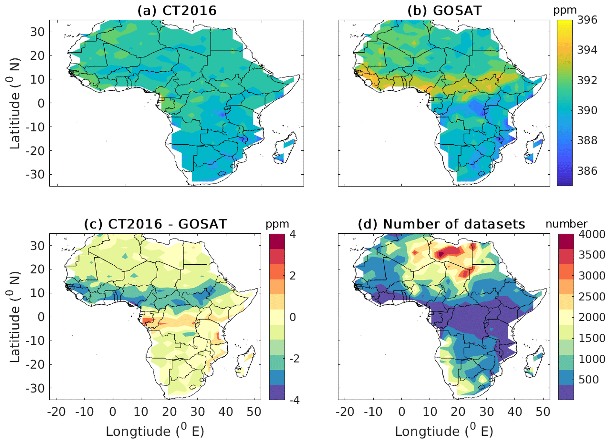
Figure 1 Distribution of 5-year averages of CT2016 (a) and GOSAT (b) XCO₂ and their difference (c) gridded in 3⁰×2⁰ bins over Africa's Land mass; and the total number of datasets at each grid from the GOSAT observations (d).

Figure 2a shows differences between CT2016 and GOSAT XCO₂, which ranges from −4 to 3 ppm. Out of 100 % occurrence, more than 90 % of observed differences are within ±2 ppm. The mean difference between CT2016 and GOSAT means is about −0.27 ppm, with the standard deviation of 0.98 ppm indicating better regional consistency and low potential outliers. Moreover, a negative mean of the difference implies that XCO₂ simulated from CT2016 is lower than that of GOSAT retrievals over Africa's land mass.

Because of selection criteria which permit a difference of 3^∘ long and wide, the two datasets are not exactly at the same point. The impact of the relative distance between them should be assessed before performing any statistical comparison. Figure 2b depicted the colour-coded scatter plot of CT2016 model simulation versus GOSAT to determine whether the discrepancy between the datasets arises from the spatial mismatch. The colour code indicates the relative distance between the model and observation datasets. For these datasets the 50th percentile has a relative distance of 1.19⁰, which means 50 % of the data have a relative distance of shorter than 1.19⁰. The maximum relative distance between them is 2.12⁰. However, there is no indication that this has been the case since the scatter is not a function of the relative distance between the datasets. For example, data points with blue colour with the lowest location difference are scattered everywhere instead of along the 1:1 line. Furthermore, we found the bias of −0.26 ppm, correlation coefficient of 0.86 and RMSD of 2.19 ppm for datasets which have a relative distance shorter than 1.19⁰. On the other hand, the bias, correlation coefficient, and RMSD are −0.33, 0.86 and 2.22 ppm for those which are above 1.19⁰. These statistics confirm that there is no strong discrepancy due to our selection criteria.

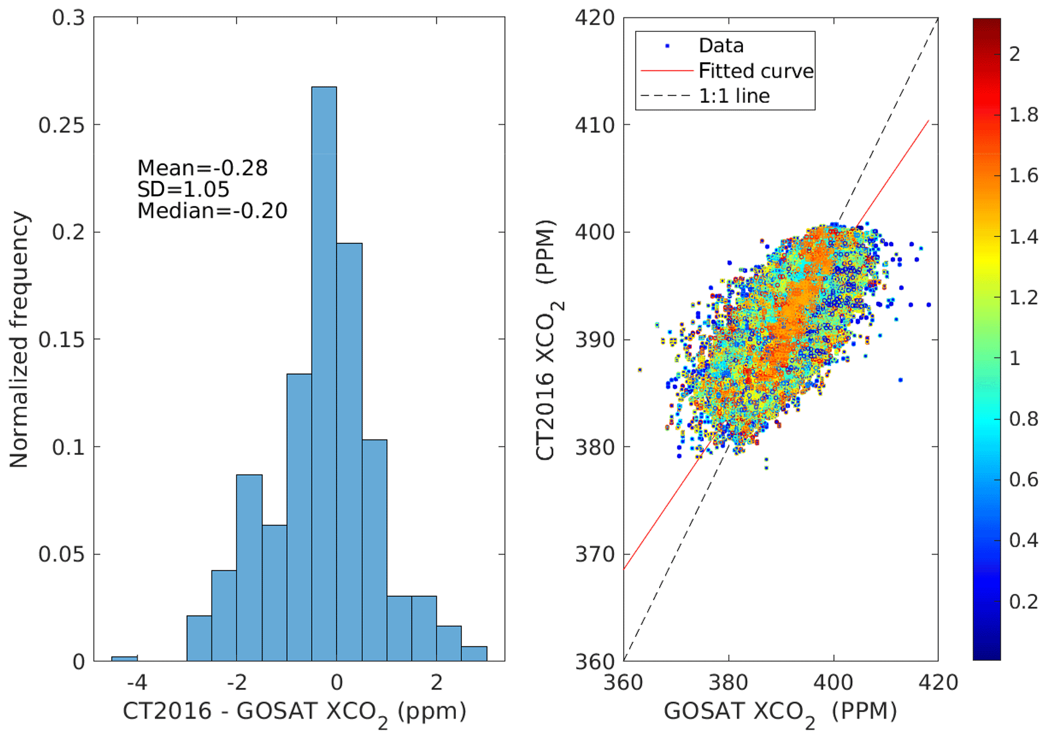
Figure 2 Histogram of the difference of CT2016 relative to GOSAT (a) and colour code scatter diagram of XCO₂ concentration as derived from CT2016 and GOSAT (b). Colour indicates the relative distance in unit of degrees as shown in the colour bar between datasets.

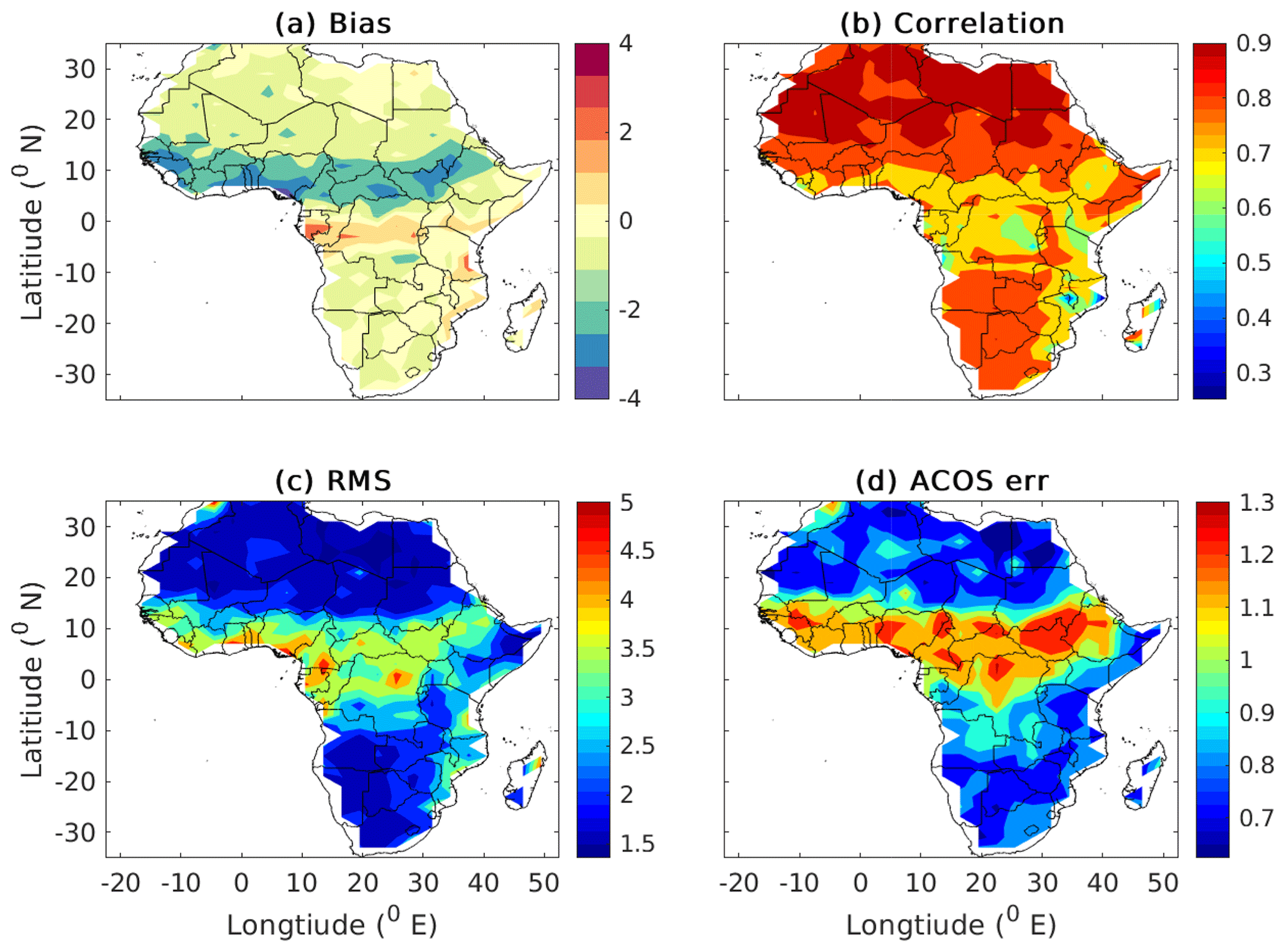
Figure 3 Spatial patterns of bias (a), correlation (b), RMSD (c) of the two datasets, and mean posteriori estimate of XCO₂ uncertainty from GOSAT (d).

Figure 3 shows a statistical comparison of XCO₂ from the CT2016 and GOSAT over Africa. The number of data used in this comparison are shown in Fig. 1d. As is depicted in Fig. 3a, the bias ranges from −4 to 2 ppm with a mean bias of $-\mathrm{0.28}\pm \mathrm{1.05}$ ppm (see Table 2). A larger negative bias of about −2 ppm was found along the annual mean position of the ITCZ, the main climatic mechanisms controlling rainfall in Africa. Systematic errors due to the ITCZ and the East African Monsoon need to be addressed well in satellite retrievals and modelling works. The correlation varies from 0.4 over some isolated pockets in Congo, Tanzania, Mozambique, Uganda, and western Ethiopia to 0.9 over the northern part of Africa above 13^∘ N, eastern Ethiopia and the Kalahari. Figure 3b depicts the correlation coefficient between GOSAT and Carbon Tracker XCO₂. The region with poor correlation also exhibits high RMSD as shown in Fig. 3c. To understand whether this discrepancy originates from model weakness alone or terrible satellite visibility when the ITCZ is present and clouds are extremely thick and widely present, we have looked at the GOSAT posterior estimates of XCO₂ error (Fig. 3d), which are high over regions where the bias and RMSD between GOSAT and Carbon Tracker XCO₂ is high. GOSAT's posterior estimate of XCO₂ error is a combination of instrument noise, smoothing error and interference error (Connor et al., 2008; O'Dell et al., 2012). This posterior estimate of XCO₂ error does not include forward model error, which may lead to underestimation of the true error of satellite XCO₂ by a factor of 2 (O'Dell et al., 2012). Therefore, part of the discrepancy is clearly linked to satellite retrieval uncertainty, which might have been amplified due to the small number of data points used to calculate the mean error of GOSAT XCO₂ measurements (see Fig. 1d). In general, the two datasets are characterized by a high spatial mean correlation of 0.83±1.20, a global offset of $-\mathrm{0.28}\pm \mathrm{1.05}$ ppm, which is the average bias, a regional precision of 2.30±1.46 ppm, which is average RMSD, and a relative accuracy of 1.05 ppm, which is the standard deviation in the bias as depicted in Table 2.

Table 2 Summary of the statistical relation between CT2016 and GOSAT observation. The statistical tools shown are the mean correlation coefficient (R), the spatial average of bias (Bias), the spatial average root mean square deviation (RMSD), the standard deviation in bias (SD of bias), GOSAT posteriori estimate of XCO₂ error (GOSAT err), the standard deviation in CT2016 XCO₂ (CT2016 SD) and the standard deviation in GOSAT XCO₂ (GOSAT SD). The number of data used in the statistics is 472 792 over 426 pixels covering the study period; the distribution at each grid point is shown in Fig. 1d. Negative bias indicates that CT2016 XCO₂ is lower than GOSAT XCO₂ values.

3.2 Comparison of monthly average time series of NOAA CT2016 and GOSAT XCO₂

Table 3 Summary of statistical relation between CT2016 and GOSAT observation. The statistical analysis was made using monthly averaged time series of 60 months (i.e. months from May 2009 to April 2014).

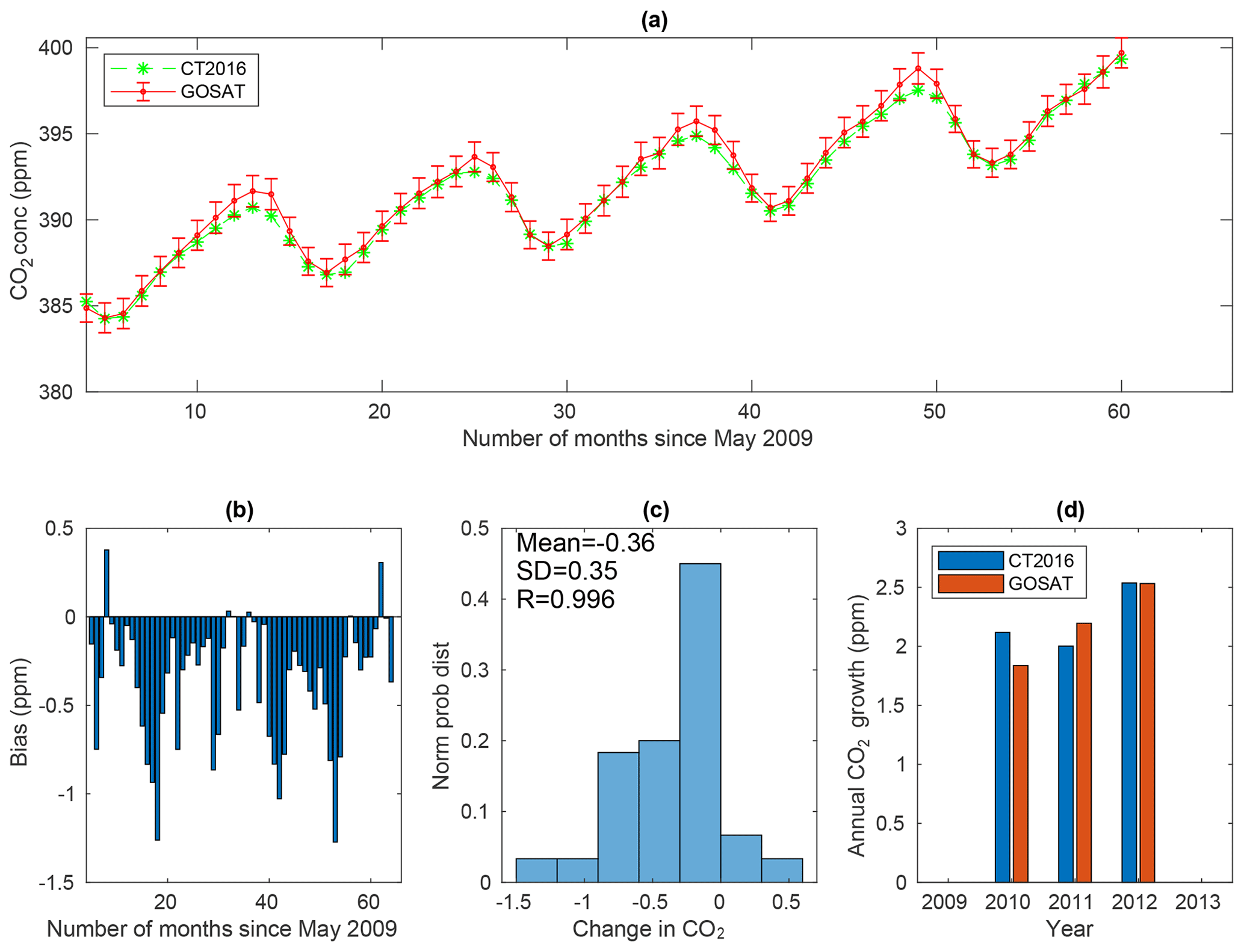
Figure 4 The monthly mean time series of CT2016 and GOSAT from May 2009 to April 2014 averaged over North Africa (a), bias associated with the monthly means (b), the histogram of difference (c) and the annual growth rate obtained by subtracting the mean from the mean of the next year (d). The error bars in (a) show the GOSAT a posteriori XCO₂ uncertainty.

Figure 5 The same as Fig. 4 but over Equatorial Africa.

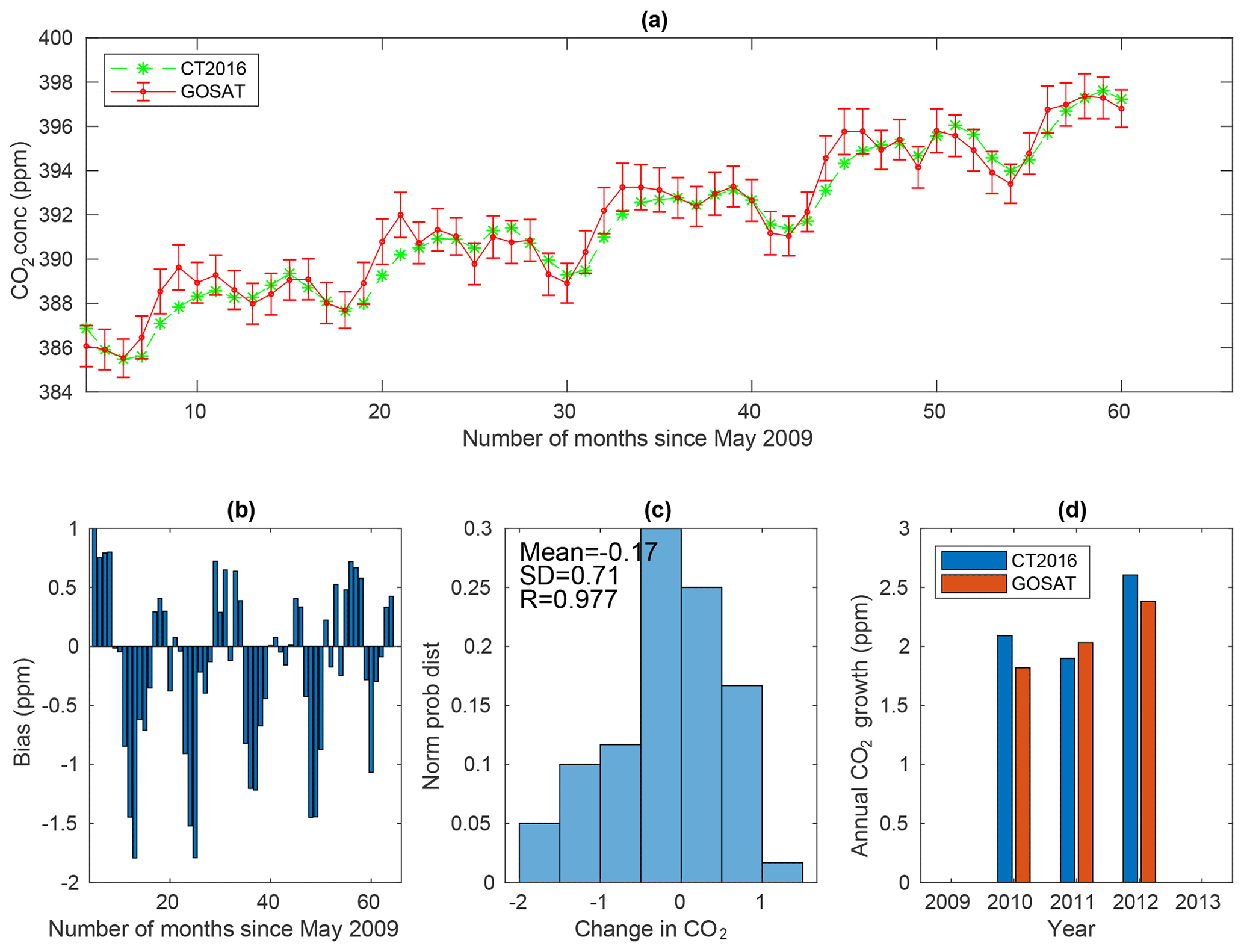
Figures 4–6 show monthly mean XCO₂ from CT2016 and GOSAT averaged over North Africa, Equatorial Africa, and Southern Africa respectively. Figures 4a–6a depict the existence of an overall very good agreement for the monthly averages with respect to amplitudes and phases of XCO₂. However, XCO₂ from the two datasets slightly disagree in capturing the seasonal cycle over Southern Africa.

Figure 6 The same as Fig. 4 but over Southern Africa.

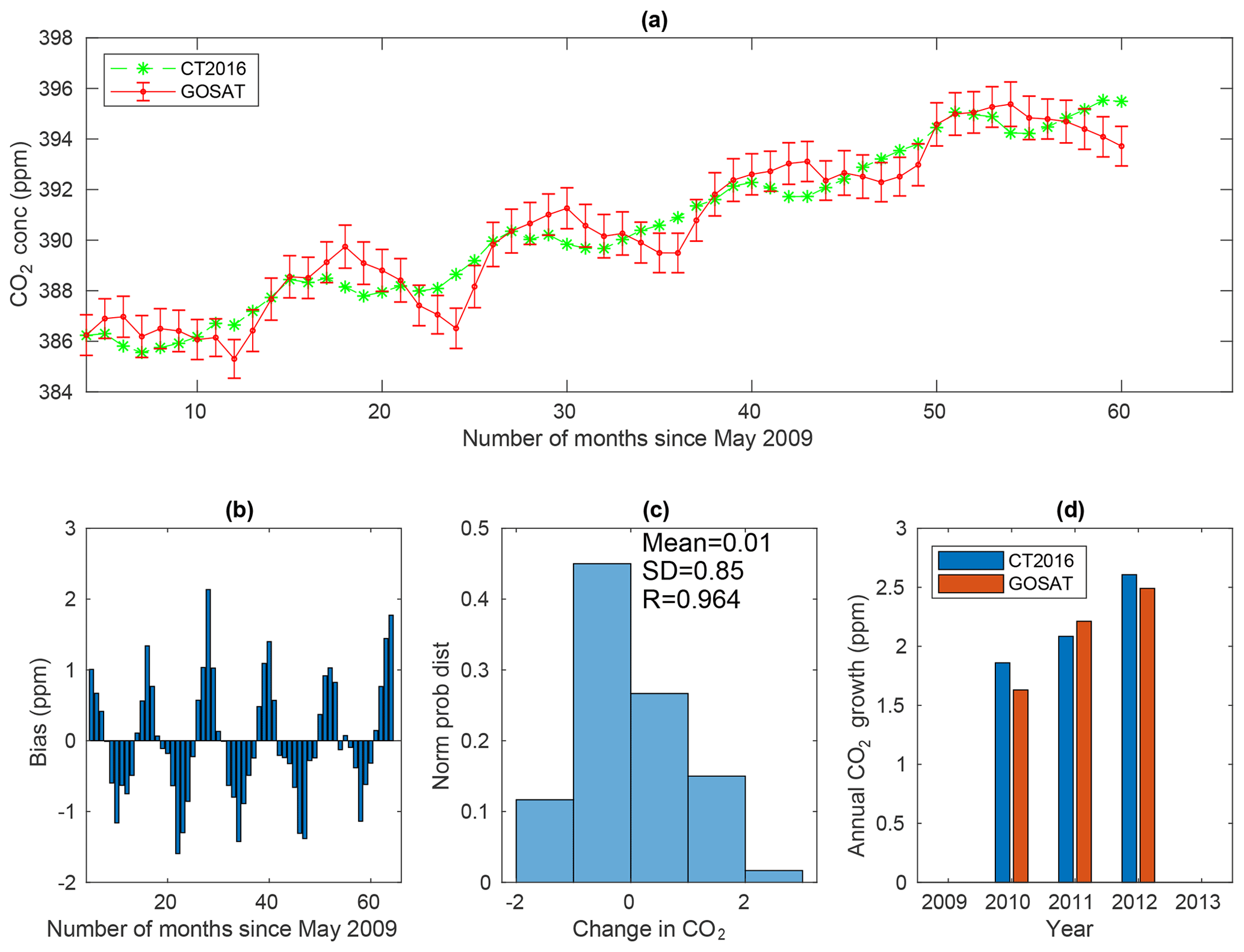
Figure 4a shows that XCO₂ concentration reaches maximum in April and minimum in September over North Africa. Consistent with this evidence, other authors (e.g. Zhou et al., 2008) have indicated the presence of strong absorption of CO₂ by vegetation during August in the Northern Hemisphere. This is the most likely the cause of the minimum concentration observed during September over North Africa. Both datasets show a concentration of XCO₂ increases from October to April and decreases from May to September (see also Table 4). Moreover, the two datasets show a monthly mean regional mean bias of −0.36 ppm with a correlation of 1.0 and a small root mean square deviation of 0.36 ppm (see Table 3).

Figure 5a shows that XCO₂ concentration reaches maxima (392.99 ppm) for CT2016 in March and (393.53 ppm) for GOSAT in January and minima (389.56 ppm for CT2016 and 389.32 ppm for GOSAT) in October over Equatorial Africa. The largest monthly mean difference of −1.34 ppm and the smallest of −0.05 ppm between the two datasets were observed in December and in April respectively (Table 4). Moreover, both datasets show that concentration of CO₂ increases from October to March, while it decreases from June to October. This similarity in the seasonal variability of the two datasets shows that they are in good agreement in terms of amplitude and phase. In addition, the two datasets show a monthly average regional average bias of −0.17 ppm, correlation of 0.98 and a small root mean square deviation of 0.71 ppm over Equatorial Africa (see Table 3). Figure 6a shows maximum XCO₂ concentration in April (391.04 ppm) for CT2016 and in October (391.28 ppm) for GOSAT and minimum in May (389.30 ppm) for CT2016 and (388.46 ppm) for GOSAT over Southern Africa. The largest monthly mean difference of 1.53 and 0.03 ppm between the two datasets is observed in April and in July (Table 4) respectively. Both datasets show a concentration of CO₂ increases from May to July, while it decreases from October to November. However, the XCO₂ from CT2016 shows a gradually increasing trend from January to April. Conversely, GOSAT XCO₂ shows decreasing values. This is most likely the result of the fact that CT2016 simulation is more sensitive to the growing size of the sink following the rainy season. Moreover, the two datasets show a monthly mean regional mean bias of 0.07 ppm, correlation of 0.97 and RMSD of 0.87 ppm over Southern Africa (see Table 3).

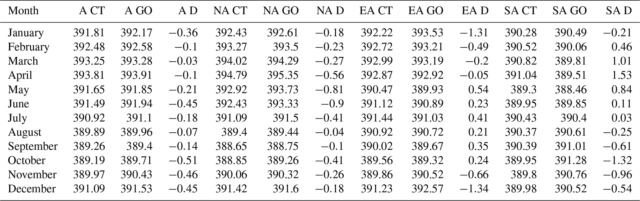
Table 4 Five-year monthly averaged XCO₂ concentration in ppm obtained from CT2016 (CT) and GOSAT (GO) and their difference CT−GO (D) in ppm over Africa (A), North Africa (NA), Equatorial Africa (EA) and Southern Africa (SA).

Figures 4b–6b show regional averaged bias in the monthly mean XCO₂ from CT2016 and GOSAT. Figure 4b shows the presence of seasonally varying negative bias over North Africa. A high ($<-\mathrm{0.5}$ ppm) negative bias in dry seasons (April to June) and low (≧−0.1 ppm) negative bias in wet seasons (August to September) are observed. Moreover, the strength of the bias increases from February to June. Conversely, the bias decreases from June to September. Similarly, Figs. 5b and 6b show seasonally fluctuating bias. For example, Fig. 6b shows a positive bias from February to July and negative bias from August to December over Southern Africa.

Figures 4c–6c show the histogram of difference. The mean difference between CT2016 simulation and GOSAT observation of XCO₂ is −0.36 ppm with a standard deviation of 0.35 ppm over North Africa (see Fig. 4c); Fig. 5c presents a mean difference of −0.17 ppm with a standard deviation of 0.71 ppm over Equatorial Africa and Fig. 6c reveals a mean difference of 0.01 ppm and a standard deviation of 0.85 ppm, which indicates that XCO₂ from CT2016 was slightly higher than that of GOSAT over Southern Africa on average. In addition, the low standard deviation of monthly mean difference over North Africa typically indicates good regional consistency between CT2016 and GOSAT. This is mainly because North Africa is dominated by the Sahara, which is a vegetation-free area, and the systematic bias due to the local atmosphere–biosphere interaction is minimum. However, the spatial mean of monthly mean bias is slightly higher (−0.36 ppm) over North Africa than over Equatorial Africa (−0.17 ppm) and Southern Africa (0.01 ppm). This is possibly due to the presence of strong local emissions from Egypt, Algeria and Libya as well as due to long-range transport from the Northern Hemisphere as reported in other studies (Williams et al., 2007; Carré et al., 2010).

Figure 7 Seasonal climatology of XCO₂ for NOAA CT2016 (left panels) and GOSAT (middle panels) and their difference (right panels).

Figures 4d–6d display the annual growth rate of XCO₂, which ranges from 1.5 to 2.7 ppm yr⁻¹. Moreover, the two datasets are consistent in determining the annual growth rate. The results are found to be in good agreement with the observed variability in the global annual growth rate from surface measurements (http://www.esrl.noaa.gov/ gmd/ccgg/trends/global.html, last access: 20 March 2018) which is 1.67, 2.39, 1.70, 2.40, and 2.51 ppm yr⁻¹ globally during 2009–2013 respectively and 1.89, 2.42, 1.86,2.63, and 2.06 ppm yr⁻¹ for Mauna Loa during 2009–2013 respectively, with error bars of 0.05–0.09 ppm yr⁻¹ for global datasets and 0.11 ppm yr⁻¹ for Mauna Loa datasets (Kulawik et al., 2016). The growth rate may not be conclusive due to the short length of the datasets used. However, it reflects how the CT and GOSAT observations perform with respect to each other.

3.3 Comparison of seasonal climatology

The seasonal cycle has important implications for flux estimates (Keppel-Aleks et al., 2012). It is important to analyse whether there are seasonally dependent biases that are affecting the seasonal cycle and whether the datasets are capturing the same seasonal cycle. The four seasons considered here are December/January/February (DJF), March/April/May (MAM), June/July/August (JJA), and September/October/November (SON). DJF corresponds to northern winter/southern summer, MAM to northern spring/southern autumn, JJA to northern summer/southern winter, and SON to northern autumn/southern spring respectively. Figure 7 shows the seasonal distributions of CT2016 (left panels) and GOSAT (middle panels) XCO₂ and their difference (CT2016−GOSAT, right panels). The distribution clearly shows that XCO₂ concentration is maximum during MAM and minimum during SON over the North Africa. On the other hand, maxima are found during SON and minima during DJF over Southern Africa. These features are in good agreement with the rainfall climatology of the Northern Hemisphere and Southern Hemisphere. Moreover, Table 5 shows seasonally varying biases. Seasonal biases affect the seasonal cycle and amplitudes, which are important for biospheric flux attribution (Lindqvist et al., 2015).

Figure 8 Histogram of difference for the seasonal XCO₂ climatology for the DJF (a), MAM (b), JJA (c) and SON (d) seasons.

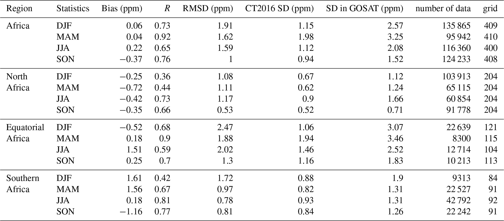
Table 5 Summary of statistical relation between CT2016 and GOSAT XCO₂: bias, correlation (R), root mean square deviation (RMSD), standard deviation of XCO₂ from CT2016 simulation (CT2016 SD), standard deviation of XCO₂ from GOSAT observation (GOSAT SD), aggregate number of coincident observations (number of data) and number of grids over the region (grid). Negative bias means CT2016 is lower than GOSAT. The statistics are on the basis of spatial averages of seasonal averages of bias, correlation, RMSD and standard deviations.

The right panels in Fig. 7 show that the seasonal mean difference (CT2016−GOSAT) ranges from −4 to 6 ppm, with a maximum difference of 6 ppm over the Gulf of Guinea and Congo during JJA. However, such a maximum difference was also observed over Southern Africa during DJF. A minimum of −4 ppm over the annual mean ITCZ region was observed during DJF and MAM. Moreover, the difference is above 1 ppm over Southern Africa during DJF and MAM (wet season of the region). This implies high spatial variability of the seasonal mean difference during different seasons (see also Table 5). It also suggests that the discrepancy between the CT2016 and GOSAT becomes significant when vegetation cover is weak during DJF and MAM (dry seasons) over North Africa.

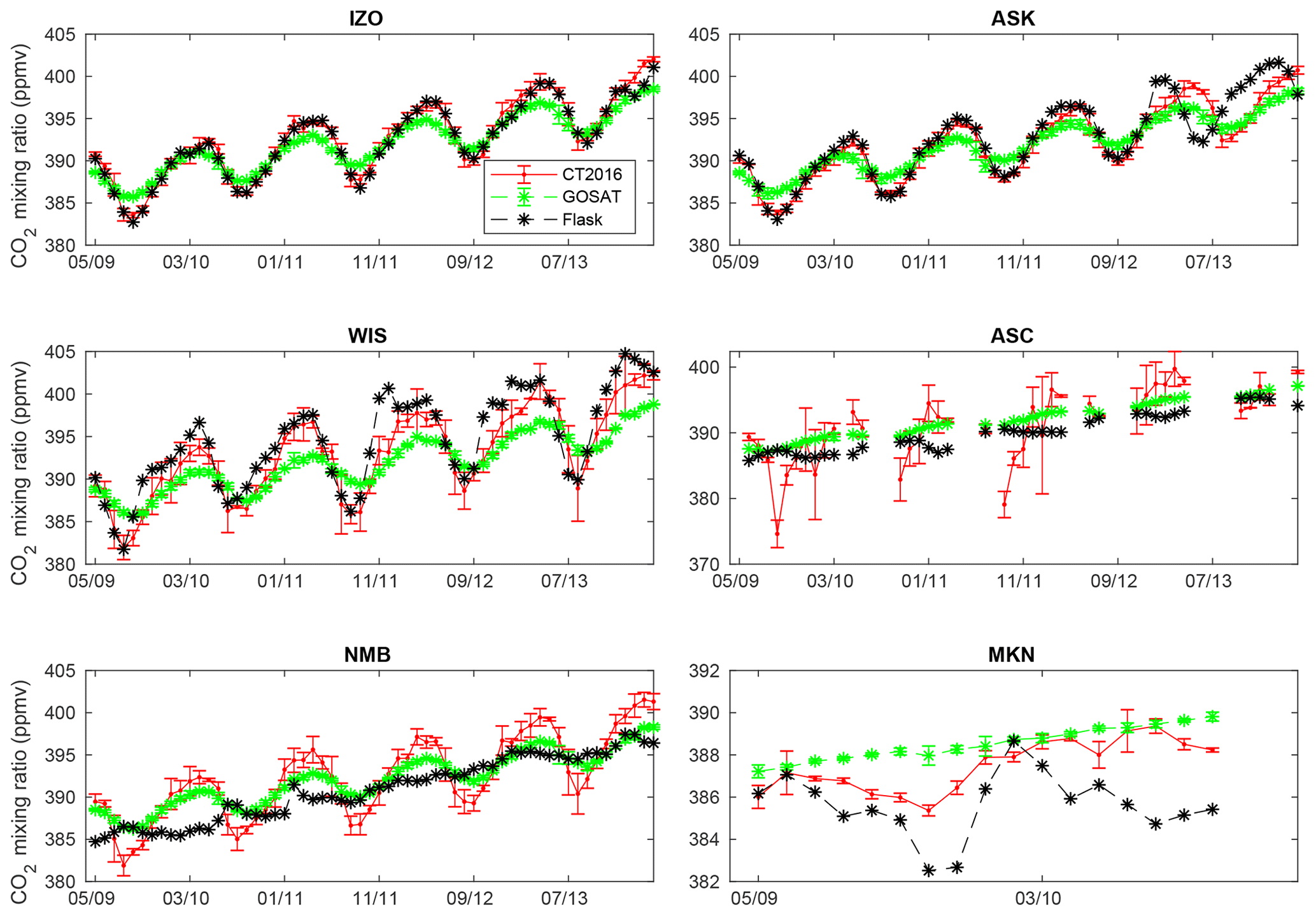
Figure 9 CO₂ time series for the coincident period for CT2016 (red), GOSAT (green) and flask (black). The standard deviation in computing the monthly mean is indicated by the vertical error bar.

During SON the seasonal difference in most of Africa's land region ranges from −2 to 1 ppm. The result implies that CT2016 simulates lower values of XCO₂ than that of GOSAT observation, indicating that there is a better spatial consistency during this season. Furthermore, during these seasons both North and Southern Africa have a moderate vegetation cover following their respective summer seasons. The two datasets show lower regional variation (i.e. only from −2 to 2 ppm) over most of Africa's land mass. However, Equatorial Africa exhibits a mean difference lower than −2 ppm during DJF and MAM. This indicates that the model tends to simulate lower than GOSAT XCO₂ over the region. Figure 7 (right panels) reveals XCO₂ from CT2016 is lower than GOSAT XCO₂ over North Africa. The underestimation of observed XCO₂ by the NOAA CT2016 model is likely related to the skill of driving ERA-Interim data as noted from previous studies. For example, Mengistu Tsidu (2012) has shown that the ERA-Interim data have a wet bias over Ethiopian highlands. Mengistu Tsidu et al. (2015) have also shown that ERA-Interim precipitable water is higher than measurements from radio-sonde, FTIR and GPS observations. Therefore, such wet bias in the driving ERA-Interim global circulation model (GCM) might have forced NOAA CT2016 to generate dense vegetation which serves as a CO₂ sink.

Figure 8 shows the mean difference between CT2016 and GOSAT XCO₂ seasonal means which ranges from −0.37 to 0.04 ppm with a standard deviation within a range of 1.00 to 1.91 ppm over the continent. The highest mean difference of XCO₂ (−0.37 ppm) occurs during SON and the lowest (0.04 ppm) occurs during MAM. Table 5 presents the summary of statistical values for the spatial mean of each season means. The comparison between the two datasets also shows there is a strong correlation (>0.5) during each season over the continent. However, there are moderate correlations (0.3 to 0.5) during DJF and MAM over North Africa and during DJF over Southern Africa. The low correlation over North Africa may be linked to a weak absorption by vegetation and a strong emission from human activities during winter as reported elsewhere (Liu et al., 2009; Kong et al., 2010). Moreover, Table 5 shows that the seasonal biases are negative over North Africa, while they are mostly positive over Equatorial and Southern Africa. Negative biases are observed during DJF and SON over Equatorial and Southern Africa respectively, implying that XCO₂ from CT2016 are lower than from GOSAT during dry seasons.

3.4 Comparison of GOSAT and CT2016 with flask observations

Comparison of GOSAT and CT2016 with flask observation is carried out over six available ground-based flask observations. For the comparison, the volume mixing ratio of CO₂ from GOSAT and CT2016 at the pressure level that corresponds to surface flask observations (see Table 1) was considered.

Monthly mean CO₂ from flask observations at IZO and ASK in North Africa shows an excellent agreement with both CT2016 and GOSAT CO₂. Moreover, CT2016 has a better sensitivity in capturing the amplitudes than GOSAT, where observations from GOSAT mostly underestimate higher values of flask CO₂ (Fig. 9). However, this agreement has deteriorated over sites in Equatorial Africa (ASC and MKN) and Southern Africa (MNB). Over MKN, CT2016 shows better correlation (0.43) than GOSAT observation (0.08). In addition, monthly amplitudes from CT2016 were closer to the flask observations, suggesting that satellite retrievals need much attention over the region. On the other hand, GOSAT observations were found to be in better agreement with flask observations over ASC. Zhang et al. (2015) also show that GOSAT data were correlated well with ground observation and found to be more centralized, having high system stability, especially over the ocean.

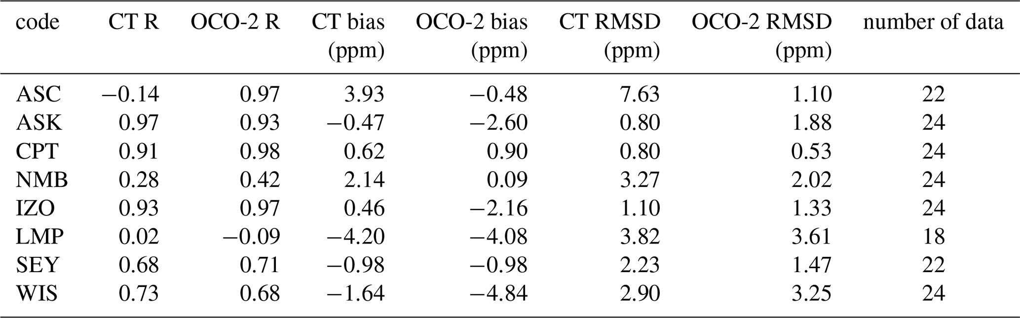
Table 6 Summary of statistical relations of CT2016 and GOSAT observation with respect to flask observations. The statistical analysis was made using monthly averages covering the period from May 2009 to April 2014).

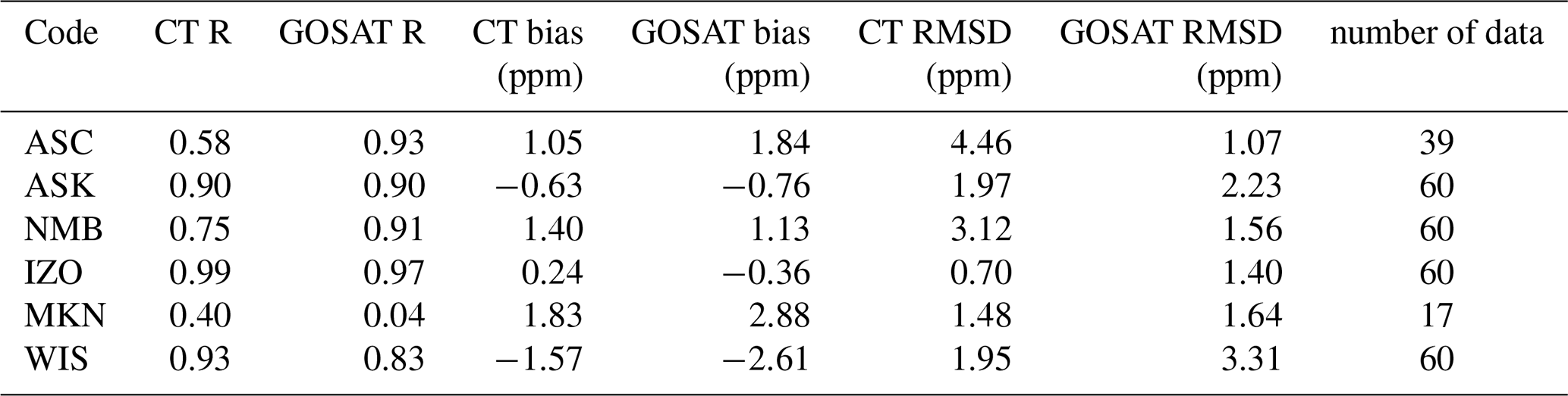
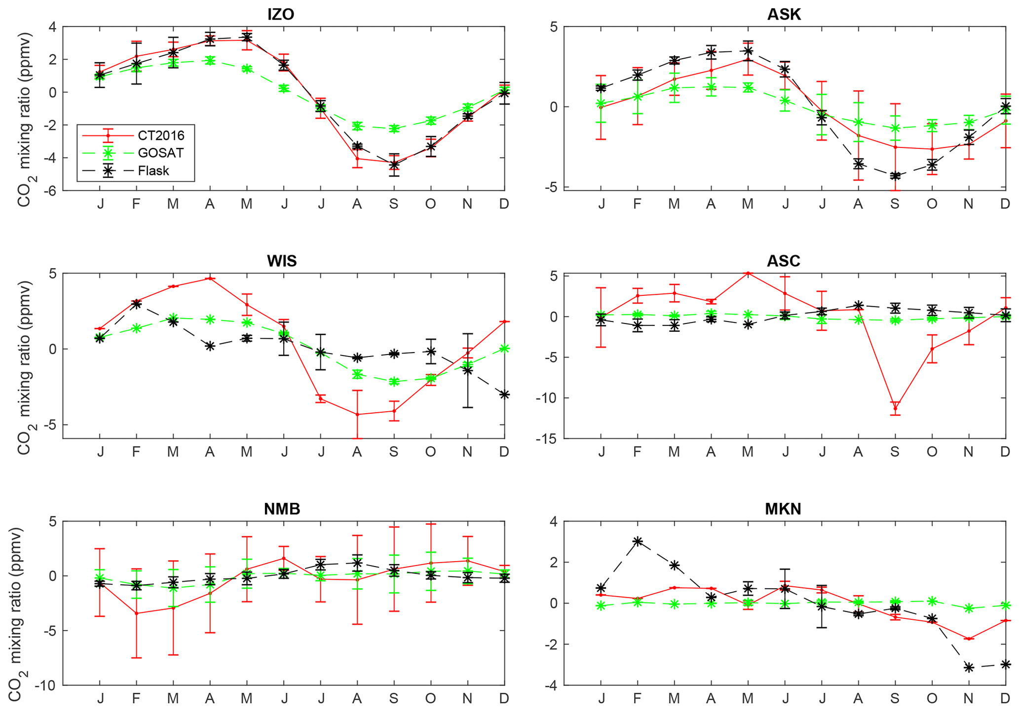
Figure 10 De-trended seasonal cycle of XCO₂ during 2009–2014 from CT2016 (red), GOSAT (green) and flask (black) observations. The standard deviation of the monthly variables is indicated by error bars.

CT2016 has a better sensitivity over IZO, ASK and NMB. Moreover, CT2016 compared better with flask observations than GOSAT over these sites; almost all flask observations are within the standard deviations of the monthly mean of CT2016. However, GOSAT observations were found to be in better agreement with flask observations than CT2016 was over WIS and ASC. On the other hand, both CT2016 and GOSAT have low sensitivity to flask observation over MKN (see Fig. 10). Similar to our previous discussion on sites in North Africa (IZO, ASK and WIS), CT2016 underestimates XCO₂ during August, September, and October (wet season) compered to GOSAT observation and overestimates XCO₂ during January to June. However, the CT2016 and the flask observations exhibit better agreement, indicating a bias in GOSAT observation during the wet season.

3.5 Comparison of mean XCO₂ from NOAA CT16NRT17 and OCO-2

The strong El Niño event that occurred during 2015–2016 provides an opportunity to compare the performance of CT16NRT17 during strong El Niño events. Because of the decline in terrestrial productivity and enhancement of soil respiration, the concentration of CO₂ increases during El Niño events (Jones et al., 2001). In this section we compare mean XCO₂ of NOAA CT16NRT17 and NASA's OCO-2 covering the period from January 2015 to December 2016.

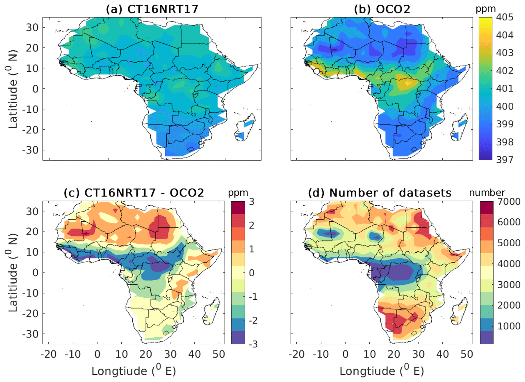
Figure 11 Distribution of 2-year average XCO₂ of CT16NRT17 (a) and OCO-2 (b) XCO₂ and their difference (c) gridded in 3⁰×2⁰ bins; and (d) the total number of datasets at each grid.

The comparison was made based on the selection criteria discussed in Sect. 2.5. Figure 11 shows the mean distribution of XCO₂ from CT16NRT17 (Fig. 11a) and OCO-2 (Fig. 11b) over Africa's land mass. CT16NRT17 shows high (>400 ppm) XCO₂ values over North Africa, while these high XCO₂ values are observed over Equatorial Africa in the case of OCO-2 observation. The two datasets show a discrepancy over Equatorial Africa, where CT16NRT17 simulates low XCO₂ values (<401 ppm), while OCO-2 observes high values of XCO₂ (>401 ppm). Both datasets show moderate XCO₂ values which range from 397 to 400 ppm over Southern Africa. The XCO₂ distribution from OCO-2 is consistent with the maximum CO₂ concentration reported in a past study by Williams et al. (2007), implying that the CT16NRT17 likely underestimates XCO₂ values over Equatorial Africa. It is also possible that the discrepancy is a compounded effect of OCO-2 XCO₂ positive bias over the region (O'Dell et al., 2012; Chevallier, 2015). Figure 11c shows the mean difference between the 2-year mean of XCO₂ from CT16NRT17 and OCO-2, which is in the range from −2 to 2 ppm. However, high ($<-\mathrm{2}$ ppm) negative mean difference between the two datasets over rainforest regions (Gulf of Guinea and Congo basin) and the ITCZ over eastern Africa (South Sudan and south-eastern Sudan) is observed, implying that CT16NRT17 simulates lower XCO₂ values than that of OCO-2 observation over regions where vegetation uptake is strong. Conversely, high (>1) positive mean difference over the Sahara, Somalia and Tanzania implies CT16NRT17 simulates higher XCO₂ values than OCO-2 observation where the vegetation uptake is weak. Moreover, a positive (>2) mean difference over Egypt, Libya, Sudan, Chad, Niger, Mali and Mauritania is likely due to overestimates of XCO₂ emission from local sources by CT16NRT17. Overall, the two datasets show a fairly reasonable agreement with a correlation of 0.60 and an offset of 0.36 ppm, a regional precision of 2.51 ppm and a regional accuracy of 1.21 ppm.

Table 7 Summary of the statistical relation between CT16NRT17 and OCO-2 observation. The statistical tools shown are the mean correlation coefficient (R), the average of bias (Bias), the average root mean square deviation (RMSD), the standard deviation in bias (SD of bias), mean posteriori estimate of XCO₂ error from OCO-2 (OCO-2 err), the standard deviation in CT16NRT17 XCO₂ (CT16NRT17 SD) and the standard deviation in OCO-2 XCO₂ (OCO-2 SD). Positive bias indicates that CT16NRT17 is higher than OCO-2. The number of data used in the statistics is 1 659 411 over 426 pixels covering the study period; the distribution at each grid point is shown in Fig. 11d.

Figure 12a shows the histogram of 2-year mean difference, which is characterized by a positive mean of 0.34 ppm and a standard deviation of 1.21 ppm. This suggests that CT16NRT17 simulates high XCO₂ as compared to observations from OCO-2 over Africa’s land mass.

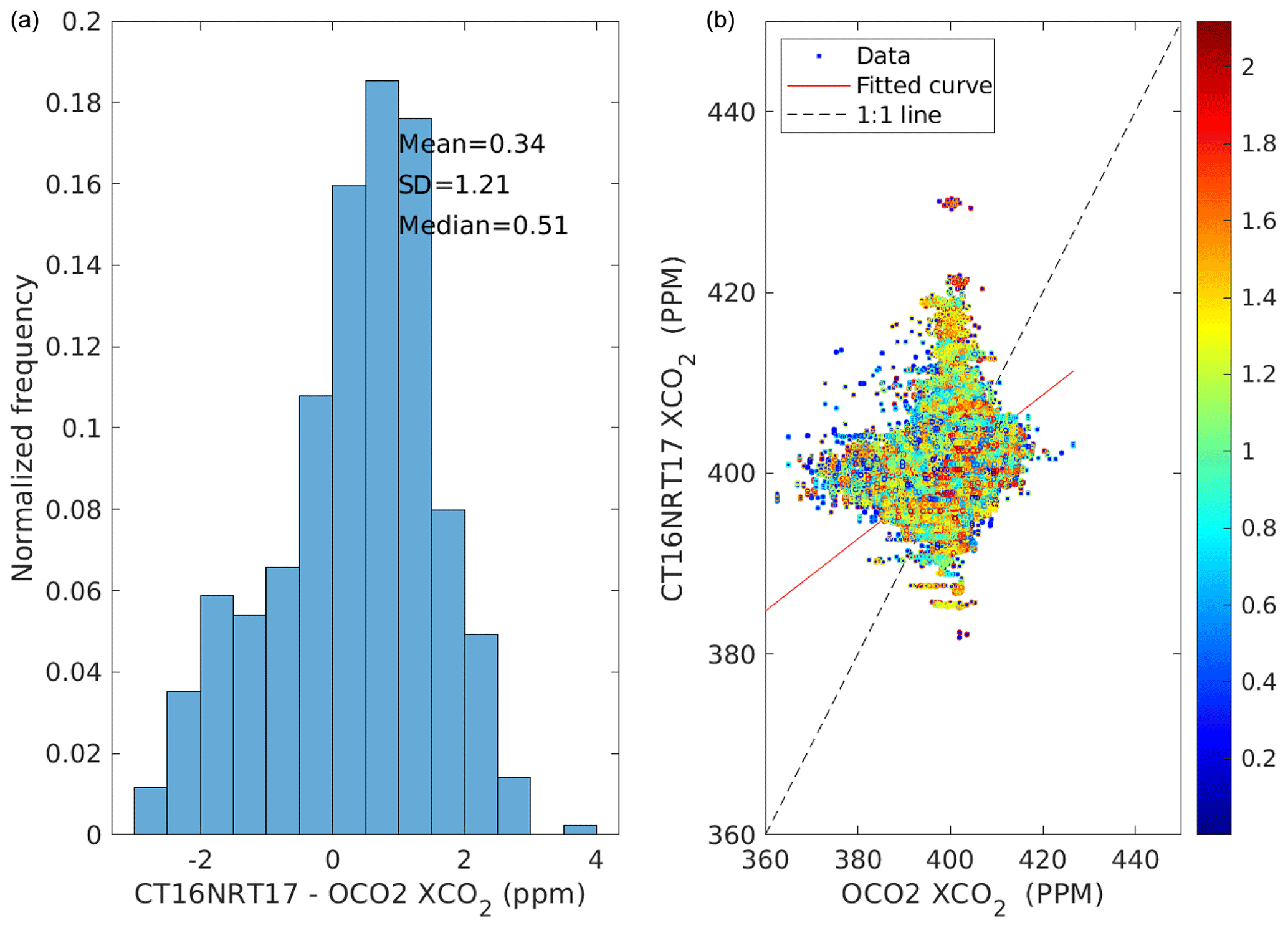
Figure 12 Histogram of the difference of CT16NRT17 relative to OCO-2 (a) and colour code scatter diagram of XCO₂ concentration as derived from CT16NRT17 and OCO-2 (b). Colour indicates the relative distance in unit of degrees as shown in the colour bar between datasets.

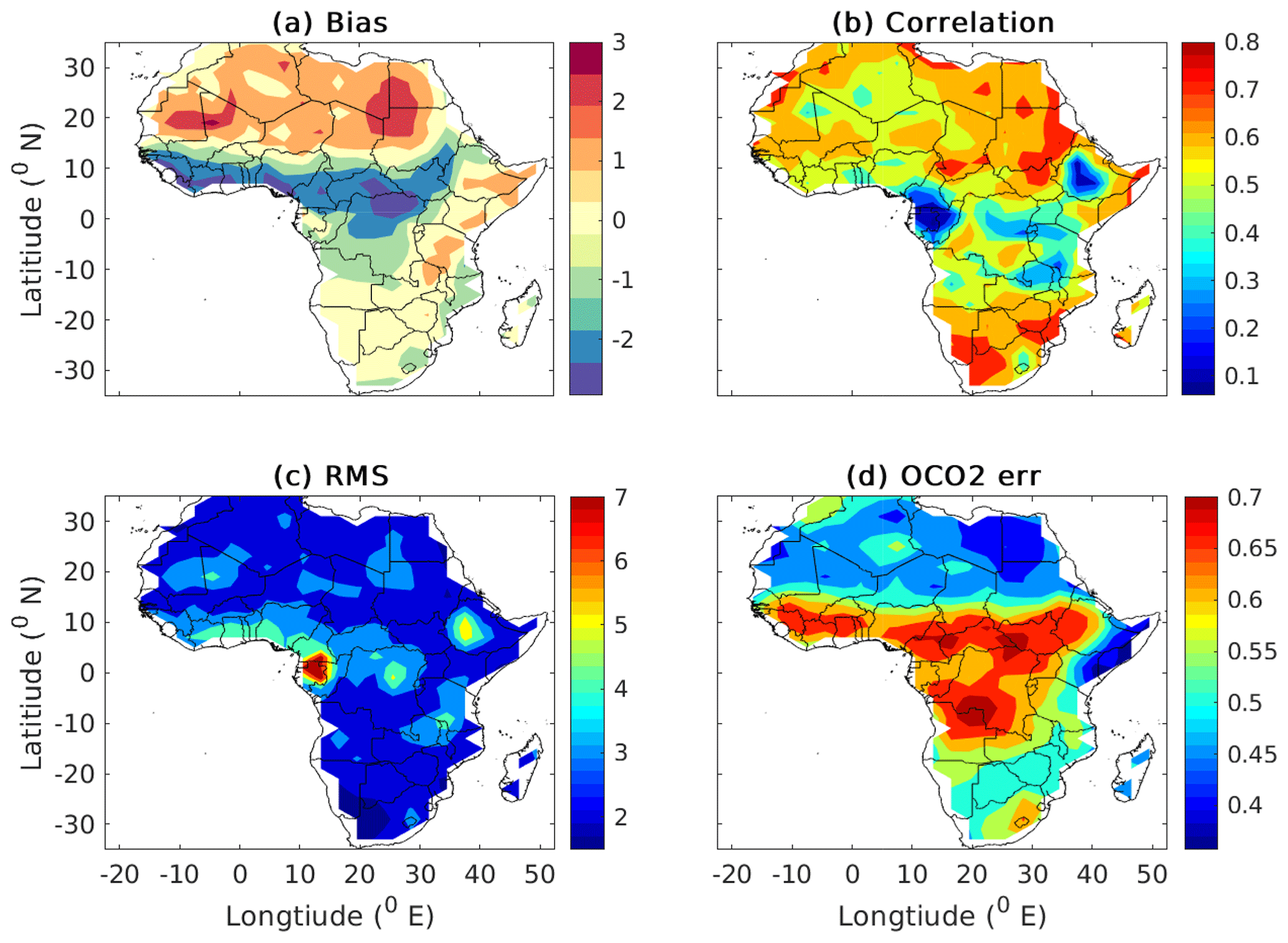
Figure 13 The bias (a), correlation (b), RMSD (c) of model and OCO-2 XCO₂ and mean posteriori estimate of XCO₂ error from OCO-2 (d).

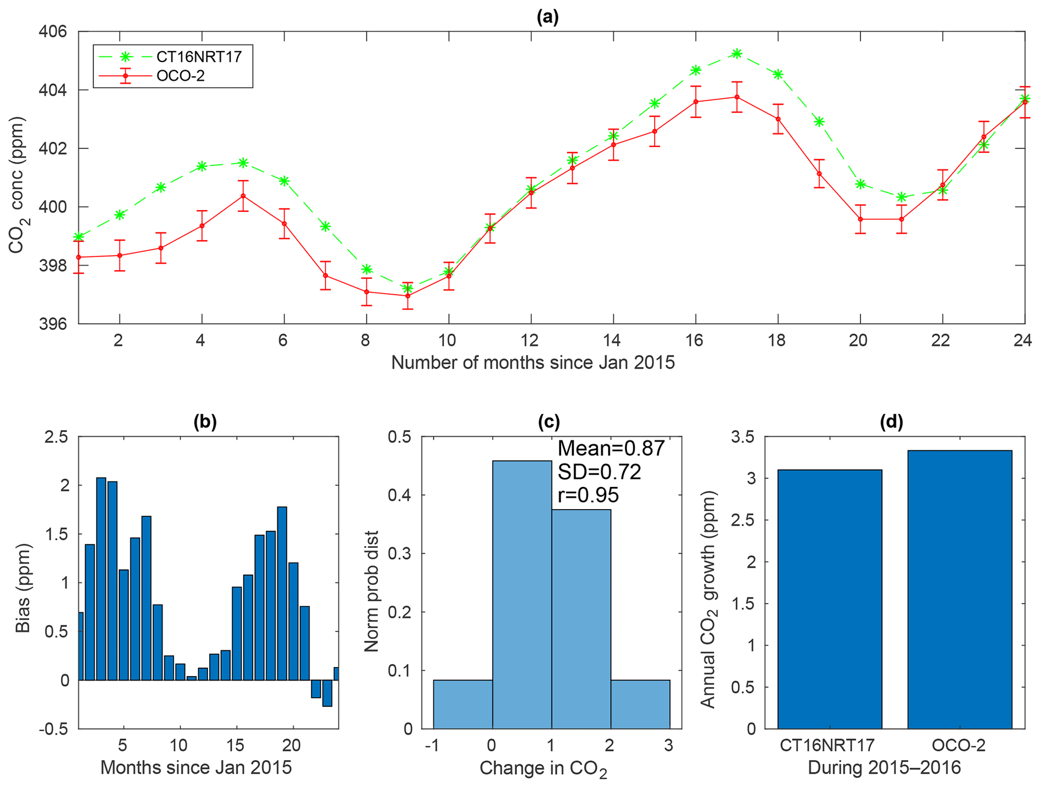
Figure 14 The monthly mean time series of CT16NRT17 and OCO-2 from January 2015 to December 2016 averaged over North Africa (a), bias associated with the monthly means (b), the histogram of difference (c) and the annual growth rate obtained by subtracting the mean from the mean of the next year (d). The error bars in (a) show the OCO-2 a posteriori XCO₂ uncertainty.

Because of the presence of spatial and temporal mismatch of some level between CT16NRT17 and OCO-2 datasets, it is important to assess the effect of relative distance between the datasets. Figure 12b shows a colour-coded distribution of the two datasets. In the figure colour codes indicate the relative distance. The random scatter of blue dots implies that the statistical discrepancies do not arise from the relative distance between the two datasets. More specifically, a statistical comparison of datasets lower and higher than the 50th percentile (1.2⁰) shows bias of 0.58 and 0.57 ppm, correlation of 0.57 and 0.57 and RMSD of 2.65 and 2.67 ppm respectively.

Table 8 Annual growth rate (AGR) of XCO₂ over Africa's land mass from CT16NRT17 and OCO-2. The results are obtained as the mean annual difference of 2015 and 2016 values.

Figure 13 shows the comparison of mean XCO₂ from CT16NRT17 and OCO-2 covering the period from January 2015 to December 2016. The number of data used are displayed in Fig. 11d. Figure 13a depicts the bias which ranges from −2 to 2 ppm with a mean bias of 0.34 ppm. However, higher biases ($<-\mathrm{2}$ ppm) are observed over Equatorial Africa along the annual average location of the ITCZ. Figure 13b shows the correlation map with values from 0.2 to 0.8 over Africa's land mass. Good correlations of above 0.6 are seen over many regions of the continent, while weak correlation of less than 0.2 and higher root mean square error (>3 ppm) are observed over small pockets of the Equatorial and eastern Africa regions (see Fig. 13c). These regions also show a higher (>0.65 ppm) error in satellite retrieval (see Fig. 13d). In addition, Fig. 11d shows the number of observations are small (<1000) over these regions. This may contribute to the observed discrepancy over these regions. However, weak correlations are also observed over a wider area in North Africa such as Mauritania, Mali, Algeria and some regions of Niger, where satellite errors are low and sufficient data are obtained. Poor correlation and higher RMSD values are observed over south-western Ethiopia.

Figure 15 The same as in Fig. 14 but over Equatorial Africa.

Figure 16 The same as in Fig. 14 but over Southern Africa.

3.6 Comparison of monthly average time series of NOAA CT16NRT17 and OCO-2 XCO₂

Figures14–16 show a 2-year monthly average time series comparison of XCO₂ from CT16NRT17 and OCO-2 over North Africa, Equatorial Africa and Southern Africa respectively. Figure 14a shows the existence of good agreement between the two datasets in describing patterns over North Africa. Moreover, both datasets show a decreasing trend of XCO₂ from May to September but an increasing trend from October to April. On the other hand, consistent with the climate condition and associated CO₂ exchange, the monthly mean XCO₂ shows a maximum value of 403.37 ppm for CT16NRT17 and 402.06 ppm for OCO-2 during May. Conversely, minimum concentrations of 398.77 ppm from CT16NRT17 simulation and 398.27 ppm from OCO-2 observation are found in September. In addition, both CT16NRT17 and OCO-2 show maximum XCO₂ values (402.15 ppm for CT16NRT17 and 402.03 ppm for OCO-2) in December. These peak values in December are not surprising, because the 2015–2016 El Niño started in March 2015 and reached its peak in December 2015, which added extra CO₂ to the atmosphere (Chatterjee et al., 2017). Figure 14a also shows that XCO₂ from CT16NRT17 simulation is higher than OCO-2 observation over North Africa.

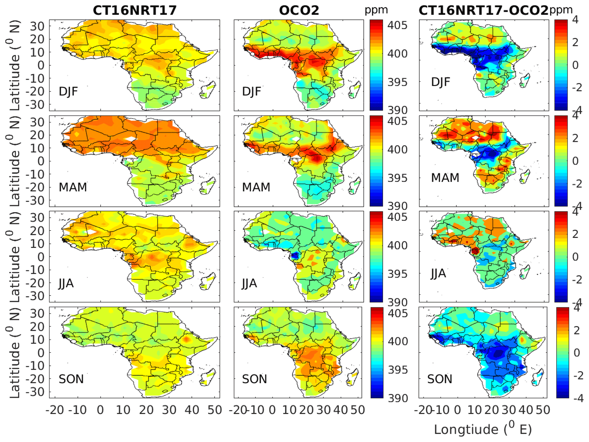
Figure 17 Seasonal mean of CO₂ for NOAA CT16NRT17 (left panels) and OCO-2 (middle panels) and their difference (right panels).

Figure 14b shows the monthly mean difference between CT16NRT17 and OCO-2 which ranges from −0.5 to 2 ppm. OCO-2 XCO₂ observations are lower than CT16NRT17 by 2 ppm during March and April 2015. Starting from August 2015, the difference between the two datasets is minimum; On the other hand, a maximum difference exceeding 1.5 ppm was observed during MAM which can be mentioned as a burning season of North Africa, as the area north of the Equator was burned mostly from March to June (Hao and Liu, 1994). The observed lower XCO₂ values from OCO-2 observations than that of CT16NRT17 simulation will be a consequence of much respiration which exceeded photosynthesis when vegetation uptake is weak following the strong El Niño and dry season over North Africa. Furthermore, intense burning of the forest during this season which will further be intensified by the strong El Niño may cause unpredicted aerosol loading, and thereby this inaccurate estimation of aerosol loading could be suggested as the most likely source for the observed discrepancy. Moreover, Fig. 14c displays a monthly mean regional mean bias of 0.87 ppm, correlation of 0.95 and root mean square deviation of 0.72 ppm between CT16NRT17 and OCO-2 XCO₂. This implies that CT16NRT17 is in good agreement with OCO-2. However, small discrepancies arose, most likely due to a strong anthropogenic emission from Nigeria, Egypt and Algeria.

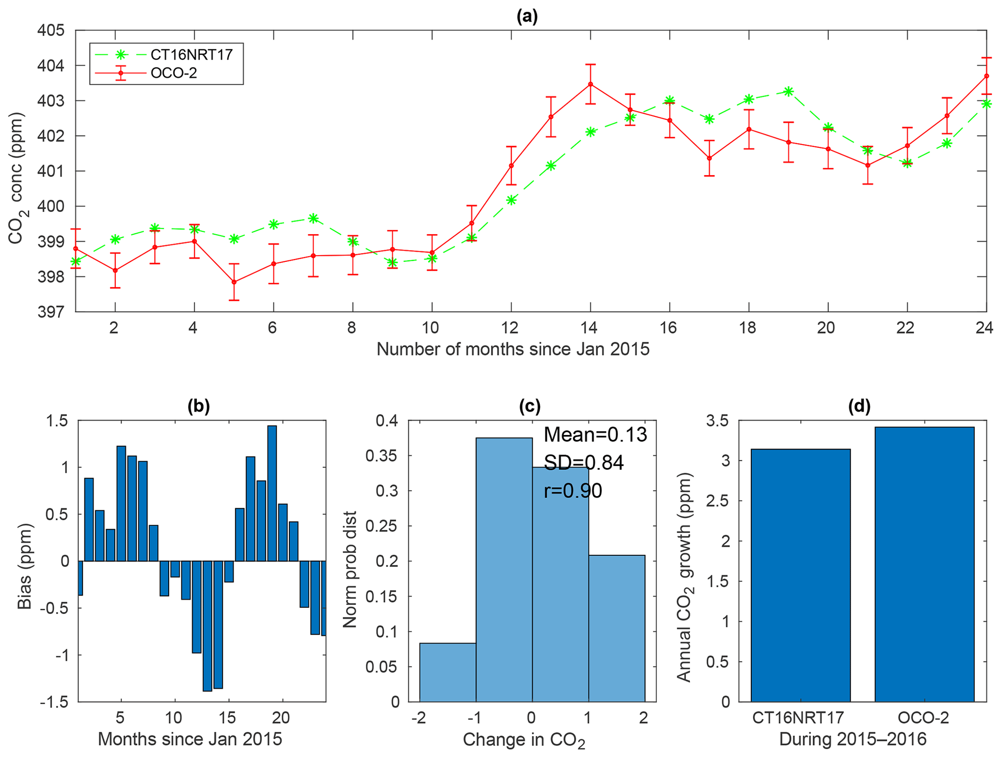
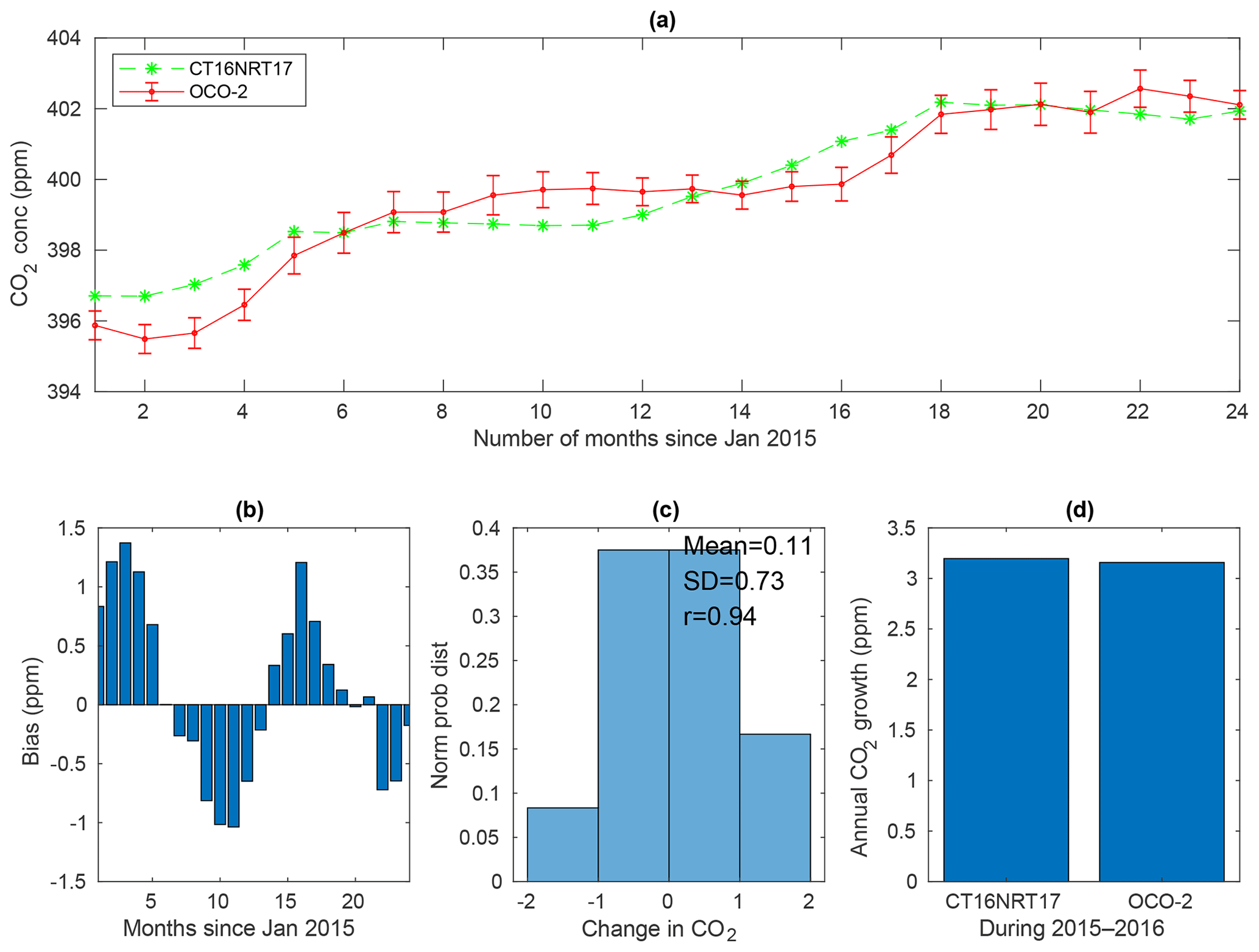
Figures 15a–16a show monthly mean time series of XCO₂ from the model and OCO-2 instrument over Equatorial Africa and Southern Africa, which are also in good agreement in terms of pattern. However, the figures show that CT16NRT17 simulations are lower than those of OCO-2 during October, November and December, whereas it is opposite during April, May and June over Equatorial Africa and Southern Africa. Figures 15b and 16b depict a seasonal bias in the monthly time series over Equatorial Africa and Southern Africa respectively. Positive biases are observed during dry seasons, while negative biases are during wet seasons. Moreover, the datasets have monthly averaged regional mean biases of 0.13 and 0.11 ppm, correlation of 0.90 and 0.94, and RMSD of 0.84 and 0.73 ppm over Equatorial Africa and Southern Africa respectively. This shows the existence of better agreement between CT16NRT17 and OCO-2 over these regions in terms of monthly average regional mean values. Figures 14d–16d show both CT16NRT17 and OCO-2 are in good agreement in estimating the annual growth rate. Patra et al. (2017) found a global mean of more than 3 Gt of CO₂ added to the atmosphere due to the strong El Niño event that occurred during 2015–2016. In agreement with this, both CT16NRT17 and OCO-2 show an annual growth rate that ranges from 3.10 to 3.42 ppm yr⁻¹ of XCO₂ over Africa's land mass (see also Table 8). However, over all regions of Africa's land mass CT16NRT17 shows a lower XCO₂ annual growth rate than those of OCO-2.

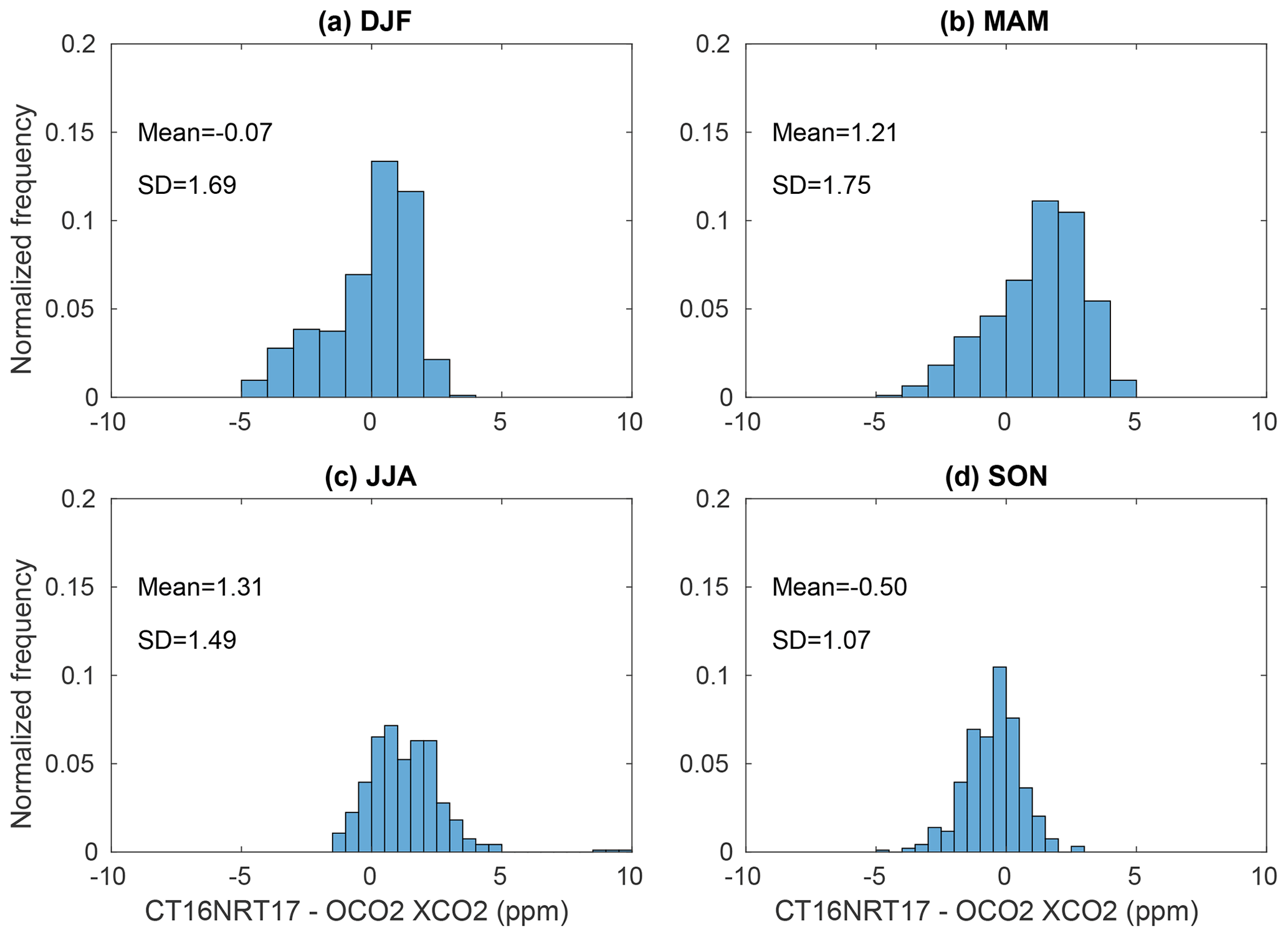
Figure 18 Histogram of difference for the seasonal CO₂ climatology for the DJF (a), MAM (b), JJA (c) and SON (d) seasons.

3.7 Comparison of seasonal means of NOAA CT16NRT17 and OCO-2 XCO₂

Figure 17 depicts seasonal means of XCO₂ over Africa's land mass from CT16NRT17 (left panels), OCO-2 (middle panels) and their difference (right panels) covering the period of January 2015 to December 2016. The white space seen over some regions (e.g. Mali during JJA) is due to insufficient coincident satellite data according to the selection criteria during these seasons. XCO₂ increases from winter to spring and then decreases from spring peak to summer minimum over the whole continent. The decrease from spring maximum to summer continued into autumn over the northern half of Africa in contrast to the southern half of Africa, which exhibits an increase in XCO₂. The decrease from spring to autumn (northward of the Equator) and until summer (southward of the Equator) is likely to be a consequence of the land vegetation awakening from dormancy of winter and partly spring. Conversely, the decomposition of died and decayed vegetation which began in autumn and continued throughout winter adds extra CO₂, leading to a maximum concentration during spring (Idso et al., 1999). In agreement with this, both CT16NRT17 and OCO-2 show maximum XCO₂ during MAM over North Africa and during SON over Southern Africa. Conversely, minimum concentrations are observed during SON over North Africa and during DJF over Southern Africa.

Figure 17 (right panels) shows the seasonal mean difference of CT16NRT17 and OCO-2. A higher mean difference greater than 1 ppm is observed over North Africa during DJF and MAM, when the vegetation cover over the region decreases and also in the presence of an intensive burning of the northern savanna during this season (Hao and Liu, 1994). This indicates that XCO₂ values from CT16NRT17 are higher than that of OCO-2 when vegetation uptake is weak and there is more fire. On the other hand, higher negative mean differences of less than −2 ppm are observed over Equatorial Africa during DJF and SON over Southern Africa. This difference between the CT and OCO-2 arises likely due to grass fires from the dry savanna. Consistent with the report by Liang et al. (2017), low seasonal variability is observed between CT16NRT17 and OCO-2 in the range from −4 to 4 ppm, with greater amplitude over North and Equatorial Africa than over Southern Africa (see Fig. 17, right panels). During dry seasons OCO-2 overestimates values over the North Africa, but it underestimates them for Southern Africa.

Figure 18 shows the histogram of seasonal mean difference of CT16NRT17 and OCO-2. The smaller standard deviations of 1.49 and 1.07 are observed during JJA and SON. On the other hand, higher standard deviations of 1.69 and 1.75 ppm are observed during DJF and MAM respectively. These results indicate that CT16NRT17 and OCO-2 show a better consistency during wet seasons, and this consistency decreases as the vegetation cover decreases over most regions of Africa's land mass during dry seasons.

3.8 Comparison of OCO-2 and CT16NRT17 with flask observations

Monthly CT16NRT17 XCO₂ has a better sensitivity over IZO and ASK both in terms of temporal pattern (phase) and amplitude than OCO-2 (see Fig. 19), where observations from OCO-2 mostly underestimate XCO₂ at the two flask sites. Over LMP and WIS, both CT16NRT17 and OCO-2 have moderate sensitivity in capturing the seasonal cycle. On the other hand, OCO-2 has a better sensitivity over ASC and SEY. In addition, XCO₂ from both CT16NRT17 and OCO-2 is found to have poor correlations with flask observations over NMB and CPT. However, OCO-2 has closer sensitivity in capturing amplitudes than CT16NRT, where CT16NRT17 overestimates XCO₂ at these flask sites. In general, CT has a better performance over sites located at high altitude (IZO, ASK) where satellite observations underestimate XCO₂. Conversely, satellite observations have better performance over low-altitude island sites (ASC and SEY) as revealed by better agreement with flask XCO₂ observations.

Figure 19 CO₂ from CT16NRT17, OCO-2 and flask observations.

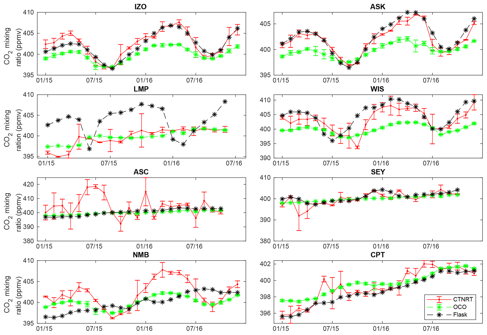
Table 9 Summary of the statistical relation of CT16NRT17 and OCO-2 observations with respect to flask observations. The statistical analysis were made using monthly averages covering the period from May 2009 to April 2014).

4 Conclusions

In this study, the GOSAT and OCO-2 XCO₂ observation values are compared with NOAA CT XCO₂ and available ground-based flask observations over Africa's land mass. Comparison between GOSAT and CT2016 was made using 5 years of datasets covering the period from May 2009 to April 2014. Comparison of OCO-2 with CT16NRT17 and eight flask observations was also made using 2 years of data during the strong El Niño event from January 2015 to December 2016. This provides an opportunity to assess the performance of OCO-2 Observation during strong El Niño events. Comparison of Carbon Tracker with the two satellites reveals biases of $-\mathrm{0.28}\pm \mathrm{1.05}$ and 0.34 ppm, correlations of 0.83±1.2 and 0.60 and root mean square deviations of 2.30±1.46 and 2.57 ppm with respect to GOSAT and OCO-2 respectively.

The monthly average time series of CT2016 over North Africa, Equatorial Africa and Southern Africa are separately compared with XCO₂ from the two satellites. CT2016 agrees well with measurements from the two instruments in terms of pattern and amplitude. However, this agreement deteriorates over Equatorial and Southern Africa in terms of amplitude. It is also found that there is a seasonally dependent bias between them which is negative during dry seasons, while it is positive during wet seasons. This indicates results of CT2016 are mostly lower than the GOSAT observation during dry seasons. High spatial mean of a seasonal mean RMSD of 1.91 during DJF and 1.75 ppm during MAM and low RMSD of 1.00 and 1.07 ppm during SON in the model XCO₂ with respect to GOSAT and OCO-2 are observed respectively, thereby indicating better agreement between CT and the satellites during autumn. CT2016 has the ability to capture monthly time series and seasonal cycles. However, XCO₂ from CT2016 is lower than GOSAT observations over North Africa during all seasons, whereas XCO₂ from CT2016 is higher than that of GOSAT over Equatorial and Southern Africa, with the exceptions of DJF over Equatorial Africa and SON over Southern Africa. In addition, CT2016 simulates lower XCO₂ than the observations over some regions (e.g. Congo, South Sudan and south-western Ethiopia) and during the summer season over the whole continent following large vegetation uptake. In contrast, XCO₂ from CT16NRT17 is higher than that of OCO-2 over North Africa, whereas it is lower than that of OCO-2 during DJF and SON over Equatorial and Southern Africa respectively. Comparison of satellite and CT with ground-based flask observation shows CT has a better performance over sites located at high altitude (IZO, ASK), as determined from good agreement with flask XCO₂ observations where satellite observations underestimates XCO₂. Conversely, satellite observations have better performance over low-altitude sites (ASC and SEY).

In general, XCO₂ from NOAA CT shows a very small bias with respect to GOSAT and OCO-2 observation over Africa’s land mass. Moreover, there is a good agreement between CT simulation and observations in terms of spatial distribution, monthly average time series and seasonal climatology. However, there are some discrepancies between the model and the two XCO₂ datasets from GOSAT and OCO-2, implying that the accuracy of the model data needs further improvements for the rainforest regions (e.g. Congo) through assimilation of in situ observations and tuning of the model through process studies.