Temperature and water vapour measurements in the framework of the Network for the Detection of Atmospheric Composition Change (NDACC)

The BASIL Raman lidar system entered the International Network for the Detection of Atmospheric Composition Change (NDACC) in 2012. Since then, measurements have been carried out routinely on a weekly basis. This paper reports specific measurement results from this effort, with a dedicated focus on temperature and water vapour profile measurements. The main objective of this research effort is to provide a characterisation of the system performance. The results illustrated in this publication demonstrate the ability of BASIL to perform measurements of the temperature profile up to 50 km and of the water vapour mixing ratio profile up to 15 km, when considering an integration time of 2 h and a vertical resolution of 150–600 m; the mean measurement accuracy, determined based on comparisons with simultaneous and co-located radiosondes, is 0.1 K (for the temperature profile) and 0.1 g kg⁻¹ (for the water vapour mixing ratio profile) up to the upper troposphere. The relative humidity profiling capability up to the tropopause is also demonstrated by combining simultaneous temperature and water vapour profile measurements.

Raman lidar measurements are compared with measurements from additional instruments, such as radiosondes and satellite sensors (IASI and AIRS), as well as with model reanalyses data (ECMWF and ECMWF-ERA). We focused our attention on six case studies collected during the first 2 years of system operation (November 2013–October 2015). Comparisons between BASIL and the different sensor/model data in terms of the water vapour mixing ratio indicate biases in the altitudinal interval between 2 and 15 km that are always within ±1 g kg⁻¹ (or ±50 %), with minimum values being observed in the comparison between BASIL and radiosonde measurements (±20 % up to 15 km). Results also indicate a vertically averaged mean mutual bias of −0.026 g kg⁻¹ (or −3.8 %), 0.263 g kg⁻¹ (or 30.0 %), 0.361 g kg⁻¹ (or 23.5 %), −0.297 g kg⁻¹ (or −25 %) and −0.296 g kg⁻¹ (or −29.6 %) when comparing BASIL with radiosondes, IASI, AIRS, ECMWF and ECMWF-ERA respectively. The vertically averaged mean absolute mutual biases are somewhat higher, i.e. 0.05 g kg⁻¹(or 16.7 %), 0.39 g kg⁻¹ (or 23.0 %), 0.57 g kg⁻¹ (or 23.5 %), 0.32 g kg⁻¹ (or 29.6 %) and 0.52 g kg⁻¹ (or 53.3 %), when comparing BASIL with radiosondes, IASI, AIRS, ECMWF and ECMWF-ERA respectively. The comparisons in terms of temperature measurements indicate mutual biases in the altitudinal interval between 3 and 30 km that are always within ±3 K, with minimum values being observed in the comparison between BASIL and radiosonde measurements (±2 K within this same altitudinal interval). Results also reveal mutual biases within ±3 K up to 50 km for most sensor/model pairs. Furthermore, a vertically averaged mean mutual bias of −0.03, 0.21, 1.95, 0.14 and 0.43 K is found between BASIL and the radiosondes, IASI, AIRS, ECMWF and ECMWF-ERA respectively. The vertically averaged absolute mean mutual biases between BASIL and the radiosondes, IASI, AIRS, ECMWF and ECMWF-ERA are 1.28, 1.30, 3.50, 1.76 and 1.63 K respectively. Based on the available dataset and benefiting from the fact that the BASIL Raman lidar could be compared with all other sensor/model data, it was possible to estimate the overall bias of all sensors/datasets: −0.04 g kg⁻¹ ∕ 0.19 K, 0.20 g kg⁻¹ ∕ 0.22 K, −0.31 g kg⁻¹ ∕ −0.02 K, −0.40 g kg⁻¹ ∕ −1.76 K, 0.25 g kg⁻¹ ∕ 0.04 K and 0.25 g kg⁻¹ ∕ −0.24 K for the water vapour mixing ratio/temperature profile measurements carried out by BASIL, the radiosondes, IASI, AIRS, ECMWF and ECMWF-ERA respectively.

1 Introduction

Water vapour is the most important atmospheric greenhouse gas, and its increasing tropospheric concentration is primarily driven (although indirectly) by human activities. Increasing concentrations of CO₂ and CH₄, which are primarily associated with fossil fuel combustion, lead to warmer tropospheric temperatures, which are responsible for increased atmospheric humidity and ultimately lead to a warmer climate (IPCC, 2007). Water vapour in the upper troposphere–lower stratosphere (UTLS) region plays a crucial role in the Earth's radiative budget, and consequently in the climate system. Its presence at these altitudes is primarily associated with two main sources: transport from the troposphere, which mainly takes place in the tropics, and the in situ oxidation of methane. Temperature and water vapour concentration changes in the UTLS result in radiative forcing alterations (e.g. Riese et al., 2012). Observations have demonstrated that the stratospheric water vapour concentration increases with increasing tropospheric temperature, implying the existence of a stratospheric water vapour feedback (Dessler et al., 2013). The strength of this feedback has been estimated to be ∼0.3 W m⁻² K⁻¹ (Dessler et al., 2013). Stratospheric water vapour also has an important role in stratospheric cloud formation, which is a key element in stratospheric ozone depletion mechanisms (di Sarra et al., 1992; Di Girolamo et al., 1994). Furthermore, stratospheric water vapour has a primary importance in the processes leading to the formation of hydrogen radicals, and consequently in stratospheric chemistry and ozone depletion mechanisms (Lossow et al., 2013).

Despite the well recognised importance of having accurate tropospheric and stratospheric water vapour and temperature profile measurements, datasets of these variables and their long-term variability are limited, especially in the UTLS region. Quality water vapour measurements in the UTLS region are provided by radiosondes or balloon-borne frost-point hygrometers. The latter is considered to be the most accurate water vapour sensor for the low humidity levels found in the UTLS region (Vomel et al., 2007). However, the global radiosonde network, which includes ∼800 stations, is quite sparse and has limited coverage in oceanic areas. Additionally, radiosondes are quite expensive and their operational launch schedule (typically two or four times per day) is not intense enough to guarantee the temporal resolution required for the above-mentioned scientific scopes. Water vapour measurements by satellite limb sounders, both in the infrared and microwave domains, have demonstrated an inadequacy with respect to both time and horizontal resolution (Griessbach et al., 2016; Hurst et al., 2014). Similar considerations apply to temperature profiling, with the main sensors covering the upper troposphere and the stratosphere being microwave and infrared satellite sounders (Thorne et al., 2005).

All of the above weather- and climate-related issues call for highly accurate measurements of both the water vapour and temperature profiles throughout the troposphere and stratosphere, with a specific focus on the UTLS region. These motivations pushed the Network for the Detection of Atmospheric Composition Change (NDACC), formerly the international Network for the Detection of Stratospheric Change (NCSC), to include water vapour and temperature lidars among its ensemble of instruments in the early 2000s. NDACC, which originally focused on the long-term monitoring of stratospheric ozone changes, has progressively broadened its priorities to include the monitoring of other atmospheric species and assessing their impacts on the stratosphere and troposphere. Atmospheric composition changes have a significant impact on the atmospheric thermal structure and this makes atmospheric temperature measurements of paramount importance for NDACC.

The University of BASILicata Raman lidar system (BASIL) entered NDACC in November 2012. The primary contribution of BASIL to NDACC is the provision of accurate routine measurements of the vertical profiles of both the water vapour mixing ratio and temperature. Water vapour profile measurements by BASIL cover the altitudinal interval from the surface up to ∼15 km, whereas temperature profile measurements cover the altitudinal interval from the surface up to the stratopause (∼50 km). The possibility of measuring down to the proximity of the surface is guaranteed by the very compact optical design of the lidar receiver, which translates into negligible differences between the overlap functions of the two ratioed Raman signals (see details in Sect. 4.2.1). Temperature measurements over such a wide altitudinal interval are possible due to the combined use of the pure rotational Raman technique (Behrendt and Reichardt, 2000), which allows the lowest 20 km to be covered, and the integration technique (Hauchercorne et al., 1992), which covers the altitudinal region from 20 km to typically 50–55 km. The combined application of these two techniques is possible owing to the presence of an overlap region (20–25 km) where both techniques work properly.

In the present research work, we illustrate and discuss temperature and water vapour profile measurements from BASIL with the purpose of assessing system performance in terms of measurement bias. Specific measurement examples are considered for this effort, which are compared with measurements from other instruments, such as radiosondes and satellite sensors (IASI and AIRS), and with model reanalyses data (ECMWF and ECMWF-ERA).

The paper outline is as follows: Sect. 2 gives a brief description of the Raman lidar set-up and its operation schedule in the framework of NDACC; Sect. 3 describes the additional profiling sensors and model data involved in the present intercomparison effort; Sect. 4 illustrates the different lidar techniques considered to measure atmospheric thermodynamic variables; Sect. 5 defines the statistical quantities used in the intercomparison for the assessment of the measurement performance; Sect. 6 illustrates the intercomparison results and provides an assessment of the performance of the sensors and models considered; and Sect. 7 summarises all of the results reported and illustrates some possible future developments of the present study.

2 The BASIL Raman lidar and its operation in the framework of NDACC

The Network for the Detection of Atmospheric Composition Change (NDACC) became operational in 1991. It includes more than 70 globally distributed, ground-based remote-sensing research stations for the observation of the physical and chemical state of the upper troposphere and stratosphere as well as their changes and for assessing the impact of these changes on global climate. Trends in the chemical and physical state of the atmosphere can be detected based on the collection of long-term databases. NDACC includes approximately 25 ground-based lidar systems distributed worldwide, which are routinely operated for the monitoring of atmospheric temperature, ozone, aerosols, water vapour and polar stratospheric clouds. To extend its research, NDACC has also established formal collaboration agreements with eight other major research networks (De Mazière et al., 2018), namely the AErosol RObotic NETwork (AERONET), the Baseline Surface Radiation Network (BSRN), the Advanced Global Atmospheric Gases Experiment (AGAGE), the Global Climate Observing System (GCOS) Reference Upper-Air Network (GRUAN), the National Aeronautics and Space Administration (NASA) Micro-Pulse Lidar Network (MPLNET), the Halocarbons and other Trace Species Network (HATS), the Southern Hemisphere Additional Ozonesonde Network (SHADOZ) and the Total Carbon Column Observing Network (TCCON).

A fundamental aspect of NDACC is represented by the high standard of quality of the data collected; we demonstrate, based on the results illustrated in this paper, that this standard is also reached by BASIL. Measurements of vertical profiles of atmospheric temperature, water vapour mixing ratio and the particle backscattering coefficient at 354.7 nm from BASIL are included in the NDACC database. BASIL is the only lidar system within the network that provides simultaneous and co-located measurements of these three atmospheric variables, with the data for these three variables being ingested into the NDACC repository and made available to the NDACC community.

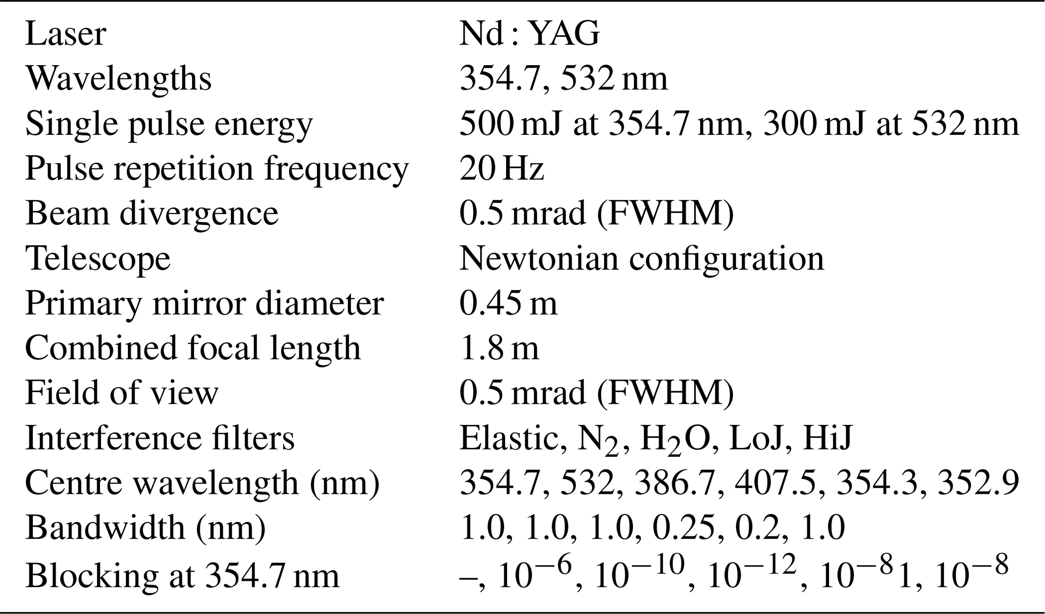
BASIL in situated in Potenza, Italy (40^∘38^′45^′′ N, 15^∘48^′29^′′ E, elevation: 730 m). The system is located in a shipping container on the roof of Scuola di Ingegneria (main building) at Università degli Studi della Basilicata. The system includes a neodymium-doped yttrium aluminium garnet (Nd : YAG) laser, with both second and third harmonic generation crystals (average power at 354.7 nm of 10 W). BASIL uses a telescope in Newtonian configuration, with a 40 cm diameter primary mirror (f∕1.8). The main characteristics of the lidar system are summarised in Table 1. BASIL performs accurate and high-resolution measurements of atmospheric water vapour and temperature, at both daytime and night-time, based on the exploitation of the vibrational and rotational Raman lidar techniques respectively, in the ultraviolet (Whiteman, 2003; Di Girolamo et al., 2009, 2004, 2006, 2018a; Behrendt and Reichardt, 2000; Bhawar et al., 2011). BASIL also carries out measurements of the particle backscattering as well as the extinction coefficient and depolarisation at 354.7 nm. Relative humidity (RH) profiles are obtained from simultaneous water vapour mixing ratio and temperature profile measurements (Di Girolamo et al., 2009b). A transportable version of the system, emitting two additional wavelengths (523 and 1064 nm), has been deployed in a variety of international field experiments (Bhawar et al., 2008; Serio et al., 2008; Wulfmeyer et al., 2008; Bennett et al., 2011; Kiemle et al., 2011; Ducrocq et al., 2014; Macke et al., 2017; Steinke et al., 2015; Di Girolamo et al., 2012a, b, 2016, 2017, 2018b). BASIL was included in NDACC with the primary aim of providing water vapour mixing ratio and temperature profile measurements. Thus, a major emphasis has been put on the collection and data processing for these variables, especially with respect to the calibration and validation efforts. In the framework of NDACC, BASIL performs routine measurements each Thursday, typically from local noon to midnight or a couple of hours after sunset.

Table 1 The main characteristics of the BASIL Raman lidar system.

In addition to a higher accuracy and better vertical resolution, a further advantage of lidar techniques with respect to traditional passive remote sensors is represented by the accurate characterisation of the random uncertainty affecting the measurements, which is available for all altitudes and each individual profile. This is determined from the signal photon number based on the application of Poisson statistics. The application of Poisson statistics to lidar signals is correct when dealing with lidar echoes acquired in both photon-counting and analogical mode. In the latter case, analogical lidar signals must first be converted into “virtual” counts. Considering an integration time of 5 min and a vertical resolution of 150 m, measurement precision at 10 km is typically 5 % for the water vapour mixing ratio and 1 K for temperature for night-time measurements. A detail description of the system set-up has been provided in several previous publications (e.g. Di Girolamo et al., 2009a, b).

2.1 Additional profiling sensors and model data involved in the intercomparison effort

2.2 IASI

The Infrared Atmospheric Sounding Interferometer (IASI), onboard the polar orbiting MetOp satellite series, is a nadir-viewing Fourier transform spectrometer measuring the radiation emitted from Earth's atmosphere in the thermal infrared region (3.2–15.5 µm or 645–2760 cm⁻¹), with an apodised spectral resolution of 0.5 cm⁻¹ (Siméoni et al., 1997 and Rabier et al., 2002; Collard, 2007). With a horizontal resolution of 12 km over a swath width of 2200 km, the IASI performs 14 sun-synchronous orbits with overpasses at 09:30 LT (local time), ensuring global coverage twice per day. The main objective of IASI is to provide accurate and high-resolution measurements of atmospheric temperature and humidity profiles. Temperature profiles are measured in the troposphere and stratosphere under clear-sky conditions, with an accuracy of 1 K and a vertical and horizontal resolution of 1 and 25 km in the lower troposphere respectively. Humidity profiles are measured in the troposphere under cloud-free conditions, with an accuracy of 10 % and a vertical and horizontal resolution of 1–2 and 25 km respectively (Wulfmeyer et al., 2005). Such performance may have a major impact on many scientific areas, especially on numerical weather prediction, where at present only IASI radiances are directly assimilated. IASI also provides measurements of trace gas concentrations, land and sea surface temperature, and emissivity and cloud properties. For the purpose of this paper, we used the IASI L2 TWT data product, available via EUMETCast, which contains atmospheric temperature and humidity profiles at 101 pressure levels and surface skin temperature. Profiles are provided at single IASI footprint resolution, with a horizontal resolution at nadir of about 25 km. The quality of the vertical profiles retrieved in cloudy instantaneous fields of view is strongly dependent on the cloud properties available in the IASI CLP product and from co-located microwave measurements.

2.3 AIRS

The Atmospheric Infrared Sounder (AIRS), launched aboard NASA's Aqua EOS satellite in 2002, is a hyper-spectral sensor including 2378 infrared channels and 4 visible/near-infrared channels, covering the spectral interval from 3.7 to 15.4 µm (2665 to 650 cm⁻¹), with a spectral resolution λ ∕ Δλ of 1200. AIRS is operated in combination with two microwave instruments, the Advanced Microwave Sounding Unit-A (AMSU-A) and the Humidity Sounder for Brazil (HSB), which are equipped with 15 and 4 microwave channels respectively.

The combined use of this ensemble of sensors allows for the provision of global coverage, as well as accurate and high-resolution measurements of atmospheric temperature and humidity profiles. Temperature profiles are measured in the troposphere and stratosphere under clear-sky conditions, with an accuracy of 1 K and a horizontal resolution of 50 km. The vertical resolution is 1 and 4 km for tropospheric and stratospheric measurements respectively. Tropospheric humidity profiles are measured under cloud-free conditions, with a vertical resolution of 2 km and an accuracy of 15 and 50 % in lower and upper troposphere respectively. The Aqua satellite is located on a sun-synchronous orbit with a nominal altitude of 705 km and an orbiting period of 98.8 min, corresponding to ∼14.5 orbits per day. Overpasses are at 01:30 LT and 013:30 LT in the descending and ascending orbits respectively. As for IASI, AIRS provides concentration measurements for a variety of trace gases. For the purpose of this paper, we used the AIRS Version 6 Level 2 standard retrieval product, which is based on 6 min data averaging (Boylan et al., 2015).

2.4 ECMWF

Reanalysis from the European Centre for Medium-Range Weather Forecasts (ECMWF) are also considered in this intercomparison effort. Two distinct reanalysis products are considered: ERA-15 (ECMWF, 2006), covering the 15-year period from December 1978 to February 1994, hereafter referred to as ECMWF; and ERA-40 (Uppala et al., 2005), hereafter referred to as ECMWF-ERA, which was originally intended to cover a 40-year period but finally included a 45-year period from 1957 (International Geophysical Year) to 2002. This latter reanalysis makes use of a larger ensemble of archived data, which was not available at the time of the original analyses. The horizontal resolution of the dataset is ∼80 km, covering 60 vertical levels from the surface up to 0.1 hPa. It is to be specified that IASI and AIRS data, as well as a variety of additional sensors, are assimilated in the ECMWF reanalyses, which makes the ECMWF reanalyses partially dependent on IASI and AIRS data, with possible non-negligible effects on the mutual biases between the satellite and the model reanalyses data. However, the mutual biases between the radiosondes and the Raman lidar, and between these two sensors and the different satellite sensors and ECMWF reanalyses are completely unaffected by sensor/model cross-dependences, as in fact radiosondes from IMAA-CNR are not assimilated by ECMWF and the Raman lidar provides completely independent measurements, which are calibrated with unassimilated radiosonde data.

3 Lidar measurements of atmospheric thermodynamic variables

3.1 Water vapour mixing ratio

Raman lidar measurements of the water vapour mixing ratio profile have been extensively reported in the literature (Whiteman et al., 1992; Whiteman, 2003). The approach makes use of the roto-vibrational Raman lidar signals from water vapour and nitrogen molecules at the two Raman-shifted wavelengths ${\mathit{\lambda }}_{{\mathrm{H}}_{\mathrm{2}}\mathrm{O}}$ and ${\mathit{\lambda }}_{{\mathrm{N}}_{\mathrm{2}}}$ respectively. These signals, expressed as the number of detected photons from a given altitude z above station level, are given by the following expressions:

$$\begin{array}{}\text{(1)}& P_{{\mathrm{H}}_{\mathrm{2}}\mathrm{O}}\left(z\right)=P_{\mathrm{0}}{\displaystyle \frac{c\mathrm{\Delta }t}{\mathrm{2}}}{\displaystyle \frac{A_{\text{tel}}}{R^{\mathrm{2}}}}{\mathit{\eta }}_{{\mathrm{H}}_{\mathrm{2}}\mathrm{O}}\text{O}\left(z\right)n_{{\mathrm{H}}_{\mathrm{2}}\mathrm{O}}\left(z\right){\mathit{\sigma }}_{{\mathrm{H}}_{\mathrm{2}}\mathrm{O}}{T}_{{\mathit{\lambda }}_{\mathrm{0}}}\left(z\right)T_{{\mathit{\lambda }}_{{\mathrm{H}}_{\mathrm{2}}\mathrm{O}}}\left(z\right)\end{array}$$

$$\begin{array}{}\text{(2)}& P_{N_{\mathrm{2}}}\left(z\right)=P_{\mathrm{0}}{\displaystyle \frac{c\mathrm{\Delta }t}{\mathrm{2}}}{\displaystyle \frac{A_{\mathrm{tel}}}{R^{\mathrm{2}}}}{\mathit{\eta }}_{{\mathrm{N}}_{\mathrm{2}}}\text{O}\left(z\right)n_{{\mathrm{N}}_{\mathrm{2}}}\left(z\right){\mathit{\sigma }}_{{\mathrm{N}}_{\mathrm{2}}}{T}_{{\mathit{\lambda }}_{\mathrm{0}}}\left(z\right)T_{{\mathit{\lambda }}_{N_{\mathrm{2}}}}\left(z\right),\end{array}$$

where P₀ is the number of transmitted photons of each laser pulse at wavelength λ₀, c is the speed of light, A_tel is the telescope aperture area, ${\mathit{\eta }}_{{\mathrm{H}}_{\mathrm{2}}\mathrm{O}/{\mathrm{N}}_{\mathrm{2}}}$ is the overall transmitter–receiver efficiency at wavelength ${\mathit{\lambda }}_{{\mathrm{H}}_{\mathrm{2}}\mathrm{O}/{\mathit{\lambda }}_{{\mathrm{N}}_{\mathrm{2}}}}$, Δt is the laser pulse duration, $n_{{\mathrm{H}}_{\mathrm{2}}\mathrm{O}}\left(z\right)$/$n_{{\mathrm{N}}_{\mathrm{2}}}\left(z\right)$ represents the water vapour/molecular nitrogen number density, ${\mathit{\sigma }}_{{\mathrm{H}}_{\mathrm{2}}\mathrm{O}}$ ∕ ${\mathit{\sigma }}_{{\mathrm{H}}_{\mathrm{2}}\mathrm{O}}$ is the water vapour/molecular nitrogen roto-vibrational Raman cross section, and $T_{{\mathit{\lambda }}_{\mathrm{0}}}\left(z\right)$ and $T_{{\mathit{\lambda }}_{{\mathrm{H}}_{\mathrm{2}}\mathrm{O}}}\left(z\right)$ ∕ $T_{{\mathit{\lambda }}_{N_{\mathrm{2}}}}\left(z\right)$ are the atmospheric transmission profiles from surface up to the scattering volume altitude z at λ₀ and ${\mathit{\lambda }}_{{\mathrm{H}}_{\mathrm{2}}\mathrm{O}}$ ∕ ${\mathit{\lambda }}_{{\mathrm{N}}_{\mathrm{2}}}$ respectively. The water vapour mixing ratio profile, $x_{{\mathrm{H}}_{\mathrm{2}}\mathrm{O}}\left(z\right)$, can be determined from the power ratio of $P_{{\mathrm{H}}_{\mathrm{2}}\mathrm{O}}\left(z\right)$ and $P_{{\mathrm{N}}_{\mathrm{2}}}\left(z\right)$ using the following expression:

$$\begin{array}{}\text{(3)}& x_{{\mathrm{H}}_{\mathrm{2}}\mathrm{O}}\left(z\right)=K\left(z\right)\cdot {\displaystyle \frac{P_{{\mathrm{H}}_{\mathrm{2}}\mathrm{O}}\left(z\right)}{P_{N_{\mathrm{2}}}\left(z\right)}}.\end{array}$$

The calibration function K(z) is determined via a calibration procedure, which is described in detail in Di Girolamo et al. (2017), based on the comparison between simultaneous and co-located water vapour mixing ratio profiles from the lidar and an independent humidity sensor. For the purpose of this study, the estimate of K(z) is based on an extensive comparison between BASIL and the radiosonde data from the nearby CIAO station. The calibration function $K\left(z\right)=c\cdot f\left(z\right)$ includes an altitude-dependent term f(z) associated with the different atmospheric transmission by molecules and aerosols at the two wavelengths corresponding to the water vapour and molecular nitrogen Raman signals and with the use of narrow-band interference filters and the consequent temperature and altitude dependencies of $P_{{\mathrm{H}}_{\mathrm{2}}\mathrm{O}}\left(z\right)$ and $P_{N_{\mathrm{2}}}\left(z\right)$ (Whiteman, 2003). c is the calibration constant, which is an altitude-independent term obtained from the comparison of the Raman lidar signal ratio $P_{{\mathrm{H}}_{\mathrm{2}}\mathrm{O}}\left(z\right)$ ∕ $P_{{\mathrm{N}}_{\mathrm{2}}}\left(z\right)$ and, in our specific case, the radiosondes launched from the nearby IMAA-CNR station. While the calibration procedure applied to BASIL has been illustrated in previous papers (e.g. Di Girolamo et al., 2009a, b, 2017), the sensor performance assessment purposes of the present publication require a proper and detailed description of the calibration procedure applied to BASIL before the intercomparison effort reported in this paper. This is illustrated in Sect. 6.1.

3.2 Temperature

In the recent past, temperature lidar measurements have become more and more important in weather and climate studies. Several lidar techniques have been demonstrated to be effective for routine measurements (Behrendt, 2005), including the rotational Raman technique (Behrendt and Reichardt, 2000) and the integration technique (Hauchecorne and Chanin, 1980; Hauchercorne et al., 1992) among others. The rotational Raman technique, especially if implemented in the UV domain, allows for the measurement of temperature profiles typically up to the lower stratosphere, whereas the integration technique is successfully used to measure temperature profiles throughout the stratosphere and mesosphere.

The Raman lidar system considered in the present paper performs simultaneous temperature measurements using both the rotational Raman technique (up to approximately 25 km) and the integration technique (from 20 km up to approximately 50 km), with a partial superimposition of the two sounded ranges in the altitudinal interval from 20 to 25 km and with no contamination of the elastic signals due to signal-induced noise effects. To the best of our knowledge, these measurements represent the first successful demonstration of the simultaneous application of both the rotational Raman and integration lidar techniques in a single instrument in the ultraviolet spectral region, i.e. in the region where the simultaneous exploitation of these two techniques has the highest potential.

3.2.1 Rotational Raman technique

Rotational Raman lidar measurements of the atmospheric temperature profile rely on the use of the rotational Raman backscattered signals from nitrogen and oxygen molecules within two narrow spectral regions encompassing rotational lines from these two species with opposite sensitivity to temperature changes: rotational lines that are closer to the laser wavelength λ₀, characterised by lower values of the rotational quantum number J, increase in intensity with decreasing temperature, whereas rotational lines that are distant from the laser wavelength, characterised by higher values of J, show the opposite behaviour, with their intensity increasing with increasing temperature.

Atmospheric temperature measurements are obtained from the ratio of the signal including low quantum number J rotational lines, P_LoJ(z), over the signal including high quantum number J rotational lines, P_HiJ(z), with the centre wavelengths for the two signals being λ_LoJ and λ_HiJ respectively. Specifically, the atmospheric temperature profile, T(z), is obtained from the signal ratio $R\left(T\right)=P_{\text{HiJ}}\left(z\right)/P_{\text{LoJ}}\left(z\right)$, via the inversion of the following expression:

$$\begin{array}{}\text{(4)}& R\left(z\right)={\displaystyle \frac{P_{\text{HiJ}}\left(z\right[T\left]\right)}{P_{\text{LoJ}}\left(z\right[T\left]\right)}}\cong \exp \left({\displaystyle \frac{a}{T\left(z\right)}}+b\right),\end{array}$$

where a and b are two calibration constants, which can be determined based on the comparison of Raman lidar measurements with simultaneous and co-located temperature measurements from a different sensor. Thus, T(z) is obtained via the following analytical expression:

$$\begin{array}{}\text{(5)}& T\left(z\right)={\displaystyle \frac{a}{\ln R\left(z\right)-b}}.\end{array}$$

In the case of BASIL, a two-parameter calibration function is well suited for the determination of the temperature profile from the P_LoJ(z) and P_HiJ(z) as a limited number of rotational lines are in fact selected for this purpose both in the low J and high J portions of the pure-rotational Raman spectrum (Di Girolamo et al., 2006). The use of a very compact optical design for the lidar receiver significantly reduces the differences between the overlap functions of the roto-vibrational Raman signals $P_{{\mathrm{H}}_{\mathrm{2}}\mathrm{O}}\left(z\right)$ and $P_{N_{\mathrm{2}}}\left(z\right)$ used to determine the water vapour mixing ratio profile, as well as the differences between the overlap functions of the pure-rotational Raman signals P_LoJ(z) and P_HiJ(z)) used to determine the temperature profile. For the present system, this translates into the capability to extend water vapour mixing ratio and temperature profile measurement down to the proximity of the surface, with a marginal blind region corresponding to the lowest 100–150 m.

The location of the rotational Raman signals' centre wavelengths λ_LoJ and λ_HiJ was determined using a specific sensitivity study that accounted for the temperature sensitivity of the rotational lines' intensity and the variable solar background conditions (Hammann and Behrendt, 2015). In the definition of the properties of the spectral selection devises (interference filters), λ_LoJ and λ_HiJ were selected with the purpose of guaranteeing comparable performance at daytime and night-time and maximising measurement precision in the temperature range that is typically found throughout the troposphere (Di Girolamo et al., 2004). Based on this selection, when using a UV laser wavelength at λ₀=354.7 nm, λ_LoJ and λ_HiJ are located at 354.3 and 352.9 nm respectively.

3.2.2 Lidar integration technique

The atmospheric number density profile, N(z), can be determined from the elastic backscatter signal at wavelength λ₀, $P_{{\mathit{\lambda }}_{\mathrm{0}}}\left(z\right)$, based on the application of a methodology defined by Hauchecorne and Chanin (1980). This approach assumes that aerosol and cloud contributions to $P_{{\mathit{\lambda }}_{\mathrm{0}}}\left(z\right)$ are negligible, which is a hypothesis verified only in unperturbed stratospheric conditions at altitudes above 25–30 km, i.e. above the background stratospheric aerosol occasionally observed in the lower stratosphere.

Once N(z) is determined, the temperature profile can easily be derived. For this purpose the ideal gas law is considered in the following form:

$$\begin{array}{}\text{(6)}& p\left(z\right)=kN\left(z\right)T\left(z\right),\end{array}$$

with p(z) being the atmospheric pressure profile, T(z) being the atmospheric temperature profile and k being the Boltzmann constant ($\mathrm{1.38}\times {\mathrm{10}}^{-\mathrm{23}}$ J K⁻¹). The barometric altitude equation, also known as hydrostatic equation, is also considered:

$$\begin{array}{}\text{(7)}& \mathrm{d}p\left(z\right)=-\mathit{\rho }\left(z\right)g\left(z\right)\mathrm{d}z,\end{array}$$

where ρ(z) is the atmospheric mass density profile and g(z) is the gravitational acceleration. Equation (7) is valid under hydrostatic equilibrium conditions. The combination of Eqs. (6) and (7) leads to the following expression (Hauchecorne and Chanin, 1980):

$$\begin{array}{}\text{(8)}& T\left(z\right)={\displaystyle \frac{N\left(z_{\text{ref, 2}}\right)}{N\left(z\right)}}T\left(z_{\text{ref,2}}\right)+{\displaystyle \frac{M}{kN\left(z\right)}}\underset{z_{\text{ref,2}}}{\overset{z}{\int }}g\left(\mathit{\varsigma }\right)N\left(\mathit{\varsigma }\right)\mathrm{d}\mathit{\varsigma },\end{array}$$

where the atmospheric mass density profile has been expressed as $\mathit{\rho }\left(z\right)=M\times N\left(z\right)$, with M being the apparent molecular weight of atmosphere (28.97), which is considered to be constant throughout the homosphere (up to 80 km).

This algorithm can be applied starting from a reference maximum altitude, hereafter identified using the symbol z_ref,2 assuming that the atmospheric number density and temperature values at this altitude are known, i.e. N(z_ref,2) and T(z_ref,2). Imposing these boundary conditions, T(z) can be derived starting from the reference altitude z_ref,2 and progressively applying the algorithm down to lower levels. Temperature at an altitude z_ref,2+1, immediately below z_ref,2, can be expressed as follows:

$$\begin{array}{}\text{(9)}& \begin{array}{rl}T\left(z_{\text{ref,2+1}}\right)=& {\displaystyle \frac{N\left(z_{\text{ref,2}}\right)}{N\left(z_{\text{ref,2+1}}\right)}}T\left(z_{\text{ref,2}}\right)\\ +& {\displaystyle \frac{M}{kN\left(z_{\text{ref},\mathrm{2}+\mathrm{1}}\right)}}{g}_{\text{med}}{N}_{\text{med}}\mathrm{\Delta }z,\end{array}\end{array}$$

with $\mathrm{\Delta }z=z_{\text{ref,2+1}}-z_{\text{ref,2}}$ and g_med and N_med being the mean gravitational acceleration and atmospheric number density between z_ref,2 and z_ref,2+1 respectively. These can be expressed as (Behrendt, 2005)

$$\begin{array}{}\text{(10)}& g_{\text{med}}={\displaystyle \frac{g\left(z_{\text{ref,2}}\right)+g\left(z_{\text{ref,2+1}}\right)}{\mathrm{2}}}\end{array}$$

and

$$\begin{array}{}\text{(11)}& N_{\text{med}}={\displaystyle \frac{N\left(z_{\text{ref,2}}\right)-N\left(z_{\text{ref,2+1}}\right)}{\ln \frac{N\left(z_{\text{ref,2}}\right)}{N\left(z_{\text{ref,2+1}}\right)}}}.\end{array}$$

The algorithm can be applied in both the downward and upward directions. Consequently, the reference altitude z_ref,2 can be taken at the highest or lowest boundary level of the vertical region where the integration technique is applied (Behrendt, 2005). However, boundary values T(z_ref,2) and N(z_ref,2) must be known with sufficiently high accuracy if temperature profiles are to be extrapolated upward because errors build up exponentially when proceeding in this direction (Behrendt, 2005). On the contrary, when an upper reference altitude is taken and the algorithm is applied downward, errors affecting T(z_ref,2) and N(z_ref,2) do not affect the temperature profile T(z) a few kilometres below the reference altitude, with the systematic uncertainty affecting T(z) quickly reducing (Behrendt, 2005), mainly due to the stability of the equation that limits the error propagation. This is why most lidar groups, including us, usually apply this algorithm downward, typically considering values of T(z_ref,2) and N(z_ref,2) from atmospheric climatological models or satellite data (Behrendt, 2005). Systematic errors associated with the incorrect selection of T(z_ref,2) and N(z_ref,2) in the downward integration of the algorithm, given in expression Eq. (7), were investigated by Leblanc et al. (1998); they considered a value for z_ref,2 of 90 km and used (as a worst-case scenario) a reference value of T(z_ref,2) that exceeded the corresponding model value at this same altitude by 15 K. Leblanc et al. (1998) revealed that the bias was already reduced to 4 K at 80 km and to 1 K at 70 km. In real measurements, the considered value for T(z_ref,2) is expected to be much closer to its correct value. Consequently, systematic errors in the temperature profile associated with the selection of incorrect temperature boundary conditions and the application of the downward-integration technique are very small (∼1 K; Behrendt, 2005). Similar considerations are also valid for BASIL. In this case, the elastic signals extend with sufficiently high signal-to-noise up to approximately 55 km; thus, z_ref,2 is taken as equal to 55 km and the boundary values T(z_ref,2) and N(z_ref,2) are taken from the midlatitude reference atmospheric models of U.S. Standard Atmosphere (1976), considering the different seasonal options included therein (Kantor and Cole, 1962). The systematic uncertainty affecting the temperature measurement at an altitude of 5 km below z_ref,2, i.e. at 50 km, is lower than 1 K, as clearly highlighted by the results reported in Sect. 6.1 and 6.2, which reveal deviations at this altitude between BASIL and the ECMWF and ECMWF-ERA model reanalyses lower than 1 K for the case studies, i.e. considerably lower than the statistical uncertainty affecting BASIL temperature measurements at this altitude (±2 K). It is to be specified that only systematic errors associated with the selection of an incorrect value of T(z_ref,2) are to be considered, whereas those associated with the selection of an incorrect value of N(z_ref,2) are always negligible because deviations of the real atmospheric number density profiles from climatological profiles are always very small (1 %–2 %) in the altitudinal region where boundary conditions are typically selected (50–90 km). The bias values listed above are in agreement with those reported for a variety of other Rayleigh lidars operated in the framework of NDACC. Specifically, Marenco et al. (1977) reported a potential systematic uncertainty, or bias, associated with the selection of incorrect upper boundary values lower than the statistical uncertainty affecting the measurements (±2 K) for the Rayleigh lidar in Thule (Greenland). These results were obtained based on a dedicated sensitivity analysis, with the upper boundary values varied by 5 %. Leblanc et al. (1998b) reported bias values from a variety of temperature lidar systems based on Rayleigh technique included in NDACC. Specifically, temperature measurements from the CNRS-SA Rayleigh lidars at the Observatoire de Haute Provence (France) and at the Centre d'Essais des Landes were found to be characterised by a bias lower than 1 K at 55 km, whereas those from the NASA Jet Propulsion Laboratory Rayleigh lidars located at Table Mountain (California) and at Mauna Loa (Hawaii) were characterised by a bias lower than 1 K at 55 and 50 km respectively. A bias of ∼1 and ∼2 K, again associated with the selection of incorrect upper boundary values, was found to characterise the Rayleigh lidars located at Hohenpeissenberg (Germany) and Sondre Stromfjord (Greenland) respectively (Dou et al., 2009).

3.3 Relative humidity

The availability of simultaneous and co-located measurements of the water vapour mixing ratio and temperature profiles, as is the case for BASIL, makes the determination of the relative humidity profile straightforward. Relative humidity is defined as the ratio, expressed as a percentage, between the water vapour partial pressure profile e(z) and the saturated vapour pressure profile e_sat(z), i.e. RH$\left(z\right)=\mathrm{100}\times e\left(z\right)/e_{\text{sat}}\left(z\right)$. e(z) can be expressed as

$$\begin{array}{}\text{(12)}& e\left(z\right)={\displaystyle \frac{p\left(z\right)x_{{\mathrm{H}}_{\mathrm{2}}\mathrm{O}}\left(z\right)}{\mathrm{0.622}+x_{{\mathrm{H}}_{\mathrm{2}}\mathrm{O}}\left(z\right)}},\end{array}$$

with p(z) being the atmospheric pressure profile, usually taken from simultaneous measurements with other sensors (for example radiosondes) or obtained from surface pressure measurements, assuming hydrostatic equilibrium and applying the hydrostatic equilibrium equation. A commonly used expression for e_sat (z) (List, 1951) is given by

$$\begin{array}{}\text{(13)}& e_s\left(z\right)=\mathrm{6.108}\exp \left\{{\displaystyle \frac{\mathrm{17.08}\left[T\right(z)-\mathrm{273.15}]}{T\left(z\right)-\mathrm{38.97}}}\right\},\end{array}$$

with T(z) being expressed in degrees Celsius. As e_sat (z) only depends on T(z), RH(z) can be determined from BASIL measurements of $x_{{\mathrm{H}}_{\mathrm{2}}\mathrm{O}}\left(z\right)$ and T(z), based only on the knowledge of the surface pressure value.

4 Statistical quantities used for the intercomparison

In order to assess the performance of the different profiling sensors and models considered in the study, an appropriate statistical analysis has to be carried out based on the estimation of specific statistical quantities. Specifically, for each sensor/model pair, the percentage mean bias and root-mean-square (RMS) deviation profile between two sensors/models, can be determined using the following expressions (Behrendt et al., 2007a, b, Bhawar et al., 2011):

$$\begin{array}{}\text{(14)}& \begin{array}{rl}\text{bias}=& {\displaystyle \frac{\mathrm{1}}{N}}\sum _{i=\mathrm{1}}^N{\text{bias}}_i\\ =& {\displaystyle \frac{\mathrm{2}}{N}}\sum _{i=\mathrm{1}}^N\left\{{\displaystyle \frac{\sum _{z=z_{\mathrm{1}}}^{z_{\mathrm{2}}}\left[q_{\mathrm{1}}\right(z)-q_{\mathrm{2}}(z\left)\right]}{\sum _{z=z_{\mathrm{1}}}^{z_{\mathrm{2}}}\left[q_{\mathrm{1}}\right(z)+q_{\mathrm{2}}(z\left)\right]}}\right\}\end{array}\end{array}$$

$$\begin{array}{}\text{(15)}& \begin{array}{rl}\text{RMS}=& {\displaystyle \frac{\mathrm{1}}{N}}\sum _{i=\mathrm{1}}^N{\text{RMS}}_i\\ =& {\displaystyle \frac{\mathrm{2}}{N}}\sum _{i=\mathrm{1}}^N\left\{{\displaystyle \frac{\sqrt{N_z\sum _{z=z_{\mathrm{1}}}^{z_{\mathrm{2}}}\left[q_{\mathrm{1}}\right(z)-q_{\mathrm{2}}(z){]}^{\mathrm{2}}}}{\sum _{z=z_{\mathrm{1}}}^{z_{\mathrm{2}}}\left[q_{\mathrm{1}}\right(z)+q_{\mathrm{2}}(z\left)\right]}}\right\},\end{array}\end{array}$$

where q₁(z) and q₂(z) represent the water vapour mixing ratio or temperature values at altitude z for sensor/model 1 and sensor/model 2 respectively; z₁ and z₂ are the lower and upper levels of the considered altitudinal interval respectively; and N_z is the number of data points for each sensor/model in this interval. In the expressions above, we used the mean of the measurement result of the two sensors/models as a reference instead of using the measurement result of one of the two. This approach leads to more objective results than considering one of the sensors/models as a reference (Behrendt et al. (2007a, b).

For all intercomparisons reported in this paper, the bias and RMS deviation are computed over 500 m width altitudinal intervals ($z_{\mathrm{2}}-z_{\mathrm{1}}=\mathrm{500}$ m).

The index i, which has values in the range from 1 to N, identifies the specific intercomparison sample, where N is the total number of possible comparisons for each sensor/model pair. Profiles of mean bias and RMS deviation are computed taking the total number N of possible intercomparisons for each sensor/model pair into consideration. In the present intercomparison effort, we consider six case studies collected during the first 2 years of system operation in the framework of NDACC, so N is equal to 6. For the purpose of applying expressions Eqs. (14) and (15), we considered a common altitude array for each pair of sensors. Consequently, when there are different altitude arrays for the profiles compared, data from one sensor/model have to be interpolated to the other sensor/model altitude levels. A linear interpolation is used in the present effort for the water vapour mixing ratio and temperature data. Additionally, the altitudinal intervals considered in the computation of the bias and RMS deviation profiles may vary for the different sensor/model pairs depending on the vertical coverage of the sensor considered (more details in Sect. 6.3). The bias and root-mean-square deviation can be determined from expressions Eqs. (14) and (15) respectively, via their multiplication by the mean of the two profiles:

$$\begin{array}{}\text{(16)}& {\displaystyle \frac{\mathrm{2}\sum _{z=z_{\mathrm{1}}}^{z_{\mathrm{2}}}\left\{q_{\mathrm{1}}\left(z\right)+q_{\mathrm{2}}\left(z\right)\right\}}{N}}.\end{array}$$

The estimate of the bias and root-mean-square deviation between two sensors/models allows for the quantification of the mutual performance of the two, i.e. how one performances with respect to the other. The bias, which quantifies the relative accuracy of the sensors/models compared, identifies an offset between the two, which is attributable to different sources of systematic uncertainty affecting one or both sensors/models. In contrast, the root-mean-square deviation includes all possible differences between the two sensors/models, associated with both systematic and statistical uncertainties and with changes of the measured/modelled atmospheric parameter (water vapour mixing ratio or temperature) as a result of differences in the air masses considered. Based on expressions Eqs. (14) and (16), the bias and percentage bias of the sensor/model 1 vs. the sensor/model 2 have positive values when q₁(z) is larger than q₂(z), i.e. q₁(z) overestimates q₂(z) or q₂(z) underestimates q₁(z).

5 Intercomparison results

BASIL was approved to enter NDACC in November 2012 and started operations shortly afterwards. However, routine measurements on a weekly basis started only 1 year later. In this paper we report measurements performed during the 2-year period from 7 November 2013 to 5 October 2015. During this time interval BASIL collected 385 h of measurements distributed over 80 d. Lidar measurements are compared with model reanalyses (ECMWF and ECMWF-ERA40), satellite data (IASI and AIRS), and radiosondes from CNR in Tito, Italy. Figure 1 shows the location of BASIL (40^∘60 N, 14^∘85 E) as well as the footprint of AIRS (centred 40^∘50 N, 15^∘50 E, and with a size of 72 km×72 km) and IASI (centred at 40^∘89 N, 16^∘2 E, and with a size of 12 km ×12 km) and the size of the grid point of ECMWF ERA-15 and ECMWF ERA-40 (centred at 40^∘63^′′ N, 15${{}^{\circ }}^{\prime }$75^′′ E and with a size of 9 km ×9 km). The distance between BASIL and the centre point of the other sensors/models is variable, i.e. 8 km to the CIAO radiosonde launching facility at IMAA-CNR, 25 km to AIRS, 25 km to IASI and 4 km to ECMWF ERA-15 and ECMWF ERA-40.

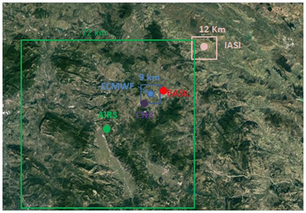
Figure 1 The location of BASIL (red dot) and the footprint of AIRS (green square centred on the green dot) and IASI (pink square centred on the pink dot), the IMAA-CNR radiosonde launching facility (purple dot) and the grid point of ECMWF ERA-15 and ECMWF ERA-40 (blue square centred on the blue dot). Map data ©2018 Google.

For the purpose of this paper, we focused our attention on six case studies collected during the first 2 years of system operation, namely 7 November, 19 December 2013, 9 October, 27 November 2014, and 2 and 9 April 2015. While a larger dataset could have been chosen, we decided to focus our attention on clear-sky cases only. In fact, clear-sky conditions represent the most suitable conditions for both water vapour and temperature measurements with Raman lidar, with water vapour profile measurements extending up to the UTLS region and temperature profile measurements extending up to 50 km. An appropriate assessment of the measurement performance based on a sensor/model intercomparison effort requires the sensors to be operated under clear-sky conditions, which is not always the case for the Raman lidar or the two passive space sensors IASI and AIRS. More specifically, the BASIL Raman lidar system does not have an all-weather measurement capability, which implies that the system is shut down in the case of precipitation. Additionally, BASIL – and this is true for all lidar systems – cannot penetrate thick clouds, as the laser beam is completely extinguished at optical thicknesses of around 2. Acceptable Raman lidar performance is still possible above thin clouds, with optical thickness less than 0.3. Thus, for the purposes of the present intercomparison effort, even the presence of high cirrus clouds makes case studies ineligible for the comparison. In other case studies, IASI and/or AIRS data were characterised by a very poor quality and unrealistic biases, which forced us to remove them from the intercomparison effort. After April 2015, the laser experienced a period during which the emitted power was reduced, possibly as a results of an unidentified internal optical misalignment. This caused a decline in the lidar's performance, which prevented us from considering measurements carried out after April 2015 within this intercomparison effort.

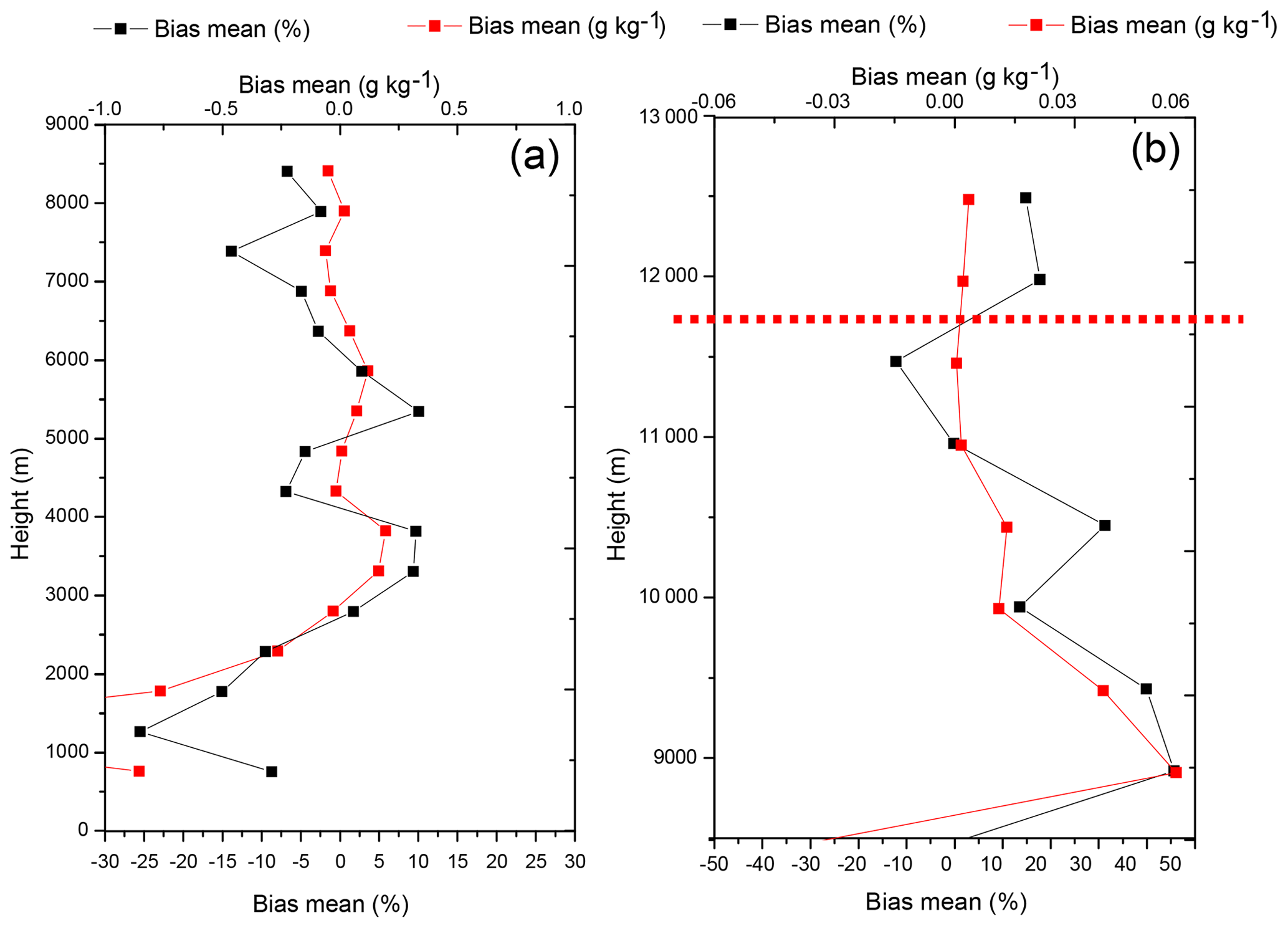
Figure 2 Vertical profiles of the water vapour mixing ratio mean bias and RMS deviation for the 11 comparisons of BASIL with the radiosondes available in the period from 9 October 2014 to 7 May 2015: (a) water vapour mixing ratio in the vertical interval between 0 and 8.5 km; and (b) water vapour mixing ratio in the vertical interval between 8.5 and 13 km. The dashed red line in (b) represents the mean tropopause altitude.

5.1 Raman lidar calibration

The Raman lidar has been calibrated based on an extensive comparison with the radiosondes launched from the nearby IMAA-CNR station, which is only 8.2 km from the Raman lidar. Launched radiosondes are manufactured by Vaisala (model RS92-SGP). For the purpose of determining the calibration constant, c, the Raman lidar and radiosonde profiles are compared over the altitudinal interval from 2.5 to 4 km, i.e. above the atmospheric boundary layer (ABL). In fact, under clear-sky conditions, the horizontal homogeneity of the humidity field above the ABL top is high enough to allow one to assume that the Raman lidar and the radiosonde are sounding the same air masses. Within this altitudinal interval, the Raman lidar signals are strong and are characterised by high signal-to-noise ratios and small statistical uncertainties. At the same time, within this low-level altitudinal interval, the horizontal drift of the radiosonde with respect to the position of lidar station is limited; thus, again, the two sensors can be assumed to be sounding the same air masses. The calibration constant, c, is obtained via a best-fit procedure applied to the Raman lidar and radiosonde data, with the value of the constant being determined by minimising the root-mean-square deviation between the single data points from the two profiles within the altitudinal interval from 2.5 to 4 km. As the Raman lidar and the radiosonde data have different altitudinal arrays, for the purpose of applying the best-fit algorithm, radiosonde data have been interpolated to the Raman lidar altitude levels.

For the purpose of determining the calibration constant, c, a specific intercomparison effort between BASIL and the radiosondes launched from IMAA-CNR was carried out in the period from 9 October 2014 to 7 May 2015. An overall number of 11 comparisons, including all coincident measurements, were possible. In this respect, it is to be specified that routine radiosonde launches started at IMAA-CNR only in October 2014; thus, intercomparisons before this date were very infrequent. Figure 2 illustrates the vertical profiles of the water vapour mixing ratio and temperature mean bias and RMS deviation for the 11 comparisons considered. The mean value of the calibration constant, $\stackrel{\mathrm{‾}}{c}$, is obtained by averaging the single calibration coefficient values from all 11 intercomparisons. The uncertainty affecting the calibration constant, σ_c, has been estimated as the standard deviation of all single calibration values from the mean value. The value of $\stackrel{\mathrm{‾}}{c}$ is found to be equal to 82.33, whereas the value of σ_c is found to be equal to 3.72. The standard deviation, expressed as a percentage ($\mathrm{100}\times {\mathit{\sigma }}_c/\stackrel{\mathrm{‾}}{c}$), is found to be equal to 4.5 %.

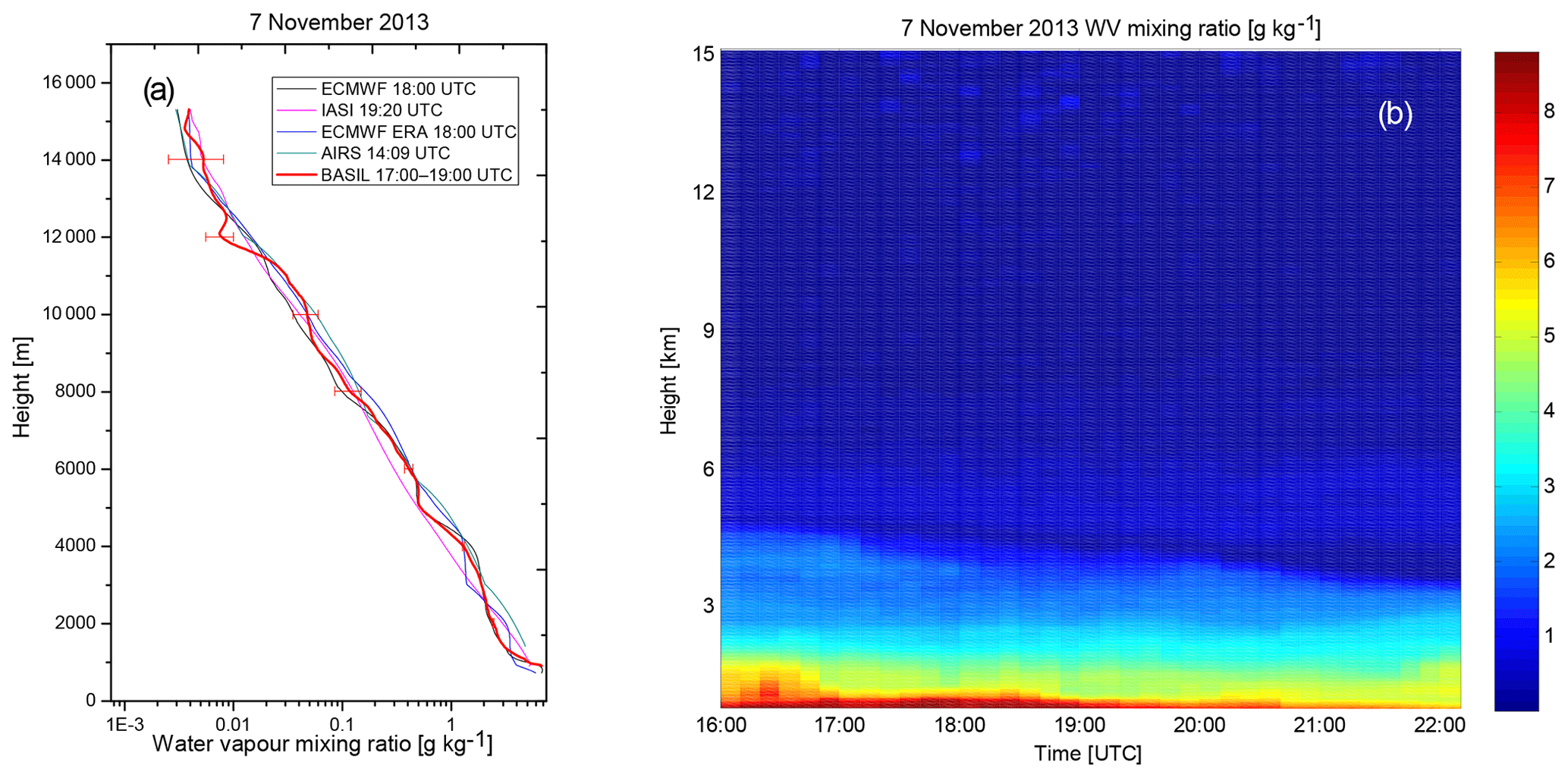
Figure 3 Water vapour mixing ratio profile as measured by BASIL over the time period from 17:00 to 19:00 UTC on 7 November 2013, as well as the closest profiles (in time) from IASI (at 19:29 UTC), AIRS (at 14:09 UTC) and the ECMWF (ERA-15 and ERA-40, at 18:00 UTC) model reanalysis (a). Time evolution of the water vapour mixing ratio profile as measured by BASIL over the interval from 16:00 to 22:00 UTC on 7 November 2013 (b).

A very similar procedure was applied to calibrate temperature measurements. However, for the purpose of determining the calibrating constants a and b, a higher altitudinal interval is considered, typically extending from 3 to 6–8 km. This is possible because pure-rotational Raman signals from N₂ and O₂ molecules are much stronger than roto-vibrational signals from water vapour molecules. Additionally, pure-rotational Raman signals are collected at wavelengths much shorter (by ∼50 nm) than the water vapour roto-vibrational Raman signal wavelength. This translates into a much smaller solar background noise affecting the signals, especially at daytime. Ultimately, N₂ and O₂ pure-rotational Raman lidar signals are characterised by much higher signal-to-noise ratios and vertical coverage and smaller statistical uncertainties than roto-vibrational signals from water vapour molecules, which allows for a higher and more extended altitudinal interval to be considered for the application of the calibration procedure. The effectiveness of the calibration procedure for temperature measurements was verified based on dedicated comparisons between calibrated Raman lidar measurements and simultaneous radiosonde profiles, which reveal the Raman lidar's capability to properly reproduce the temperature profile throughout the troposphere and stratosphere, with high accuracy at the tropopause as well. The mean and standard deviation values of the calibration constants a and b were determined to be $\stackrel{\mathrm{‾}}{a}\pm {\mathit{\sigma }}_a=\mathrm{760}\pm \mathrm{7}$ and $\stackrel{\mathrm{‾}}{b}\pm {\mathit{\sigma }}_b=\mathrm{0.97}\pm \mathrm{0.03}$ respectively.

The constancy of the calibration constant was verified over the 2-year measurement period, appearing quite stable, as neither short-term or long-term time variations were revealed. Ageing of transmitter/receiver components was verified to not produce any appreciable variation in the calibration coefficients.

With respect to the water vapour mixing ratio measurements, above the planetary boundary layer and up to 8.5 km (Fig. 2a), the mean bias is found not to exceed ±0.25 g kg⁻¹ (or ±10 %). Even above 8.5 km (Fig. 2b), bias values are very low and do not exceed ±0.06 g kg⁻¹ (or ±50 %). With respect to the temperature measurements, above the planetary boundary layer and up to 9.5 km, biases are within ±1 K.

The above-specified uncertainties affecting the water vapour measurements are in agreement with those reported for a variety of other Raman lidars operated within the framework of NDACC. Specifically, Whiteman et al. (2012) reported a 5 % uncertainty in the upper troposphere based on an extended comparison of the NASA-GSFC Raman lidar system ALVICE with Vaisala RS92 radiosondes. For the Maïdo Lidar on Réunion island, Dionisi et al. (2015) reported a relative difference below 10 % in the low and middle troposphere (2–10 km) based on a comparison with 15 co-located and simultaneous Vaisala RS92 radiosondes. The upper troposphere, up to 15 km, is found to be characterised by a larger spread (approximately 20 %), attributed to the increasing distance between the two sensors. Leblanc et al. (2012) reported water vapour mixing ratio profile measurements from the JPL Raman lidar at the Table Mountain Facility (California); these lidar have demonstrated the capability to cover the region from ∼1 km above the ground to the lower stratosphere with a precision better than 10 % below an altitude of 13 km and an estimated accuracy of 5 %. The same authors also reported very good agreement between the Raman lidar and a cryogenic frost-point hygrometer over the entire lidar range from 3 to 20 km, with a mean bias not exceeding 2 % (lidar dry) in the lower troposphere and 3 % (lidar moist) in the UTLS.

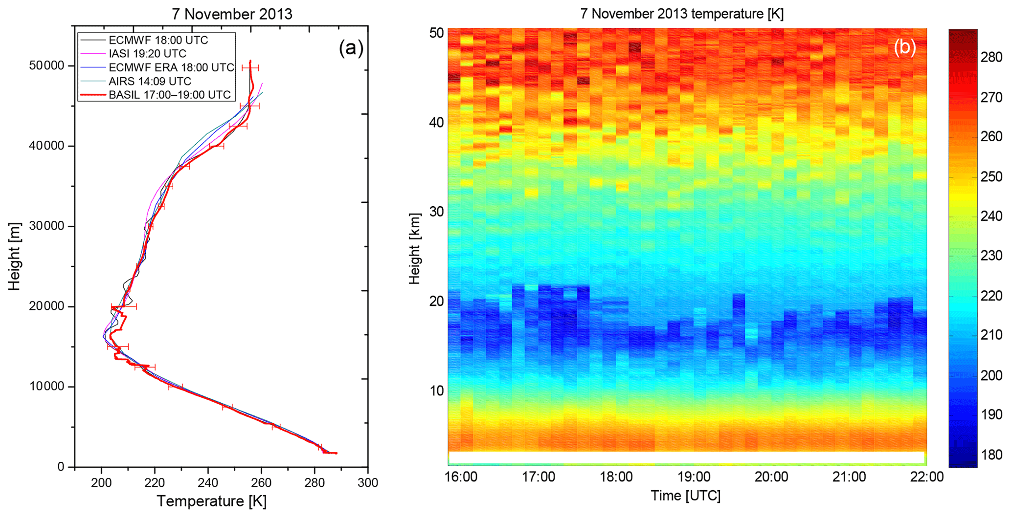
Figure 4 Vertical profile of atmospheric temperature as measured by BASIL over the time period from 17:00 to 19:00 UTC on 7 November 2013 as well as the closest profiles (in time) from IASI (at 19:20 UTC), AIRS (at 14:09 UTC) and the ECMWF (ERA-15 and ERA-40, at 18:00 UTC) model reanalysis (a). Time evolution of the atmospheric temperature profile as measured by BASIL over the interval from 18:00 to 22:00 UTC on 7 November 2013 (b).

5.2 Case studies

Figure 3a illustrates the mean water vapour mixing ratio profile measured by BASIL on 7 November 2013 over the time interval from 17:00 to 19:00 UTC. The vertical resolution of the data is 150 m from the surface up to 6 km, 300 m between 6 and 8 km, and 600 m above 8 km. The water vapour mixing ratio profile from BASIL reaches an altitude of approximately 15 km, with the capability of measuring humidity levels as low as 0.003–0.004 g kg⁻¹, with a sensitivity level of 0.001–0.002 g kg⁻¹; these two levels are defined as the mixing ratio values corresponding to 50 % and 100 % relative uncertainty in the UTLS region. The capability of reaching an altitude of 14–15 km, with a measurement detection level of 0.001–0.002 g kg⁻¹, has been verified in most of the 2 h water vapour profiles measured by BASIL in the framework of NDACC under clear-sky conditions. When considering measurements integrated in time over the entire night, the water vapour mixing ratio profile from BASIL is found to extend up to approximately 16–18 km. For this case study, the closest (in time) water vapour mixing ratio profiles from IASI (at 19:20 UTC) and AIRS (at 14:09 UTC) and the ECMWF ERA-15 and ECMWF ERA-40 model reanalysis (at 18:00 UTC) are also illustrated in Fig. 3a. In the present case study, no radiosondes were launched from the nearby CIAO launching station. The agreement between BASIL and the different sensors/models is very good, even at low altitudes where effects of water vapour heterogeneity are usually important. For this specific case study, at all altitudes between 2.5 and 15 km, deviations of BASIL vs. AIRS and IASI are lower than 0.2 g kg⁻¹ (or 40 %) and 0.1 g kg⁻¹ (or 30 %) respectively, whereas deviations between BASIL and ECMWF (ERA-15 and ERA-40) do not exceed 0.1 g kg⁻¹ (or 30 %). The mean bias of BASIL vs. AIRS, IASI, ECMWF and ECMWF-ERA40 are −16 % (or −0.13 g kg⁻¹), 7 % (or 0.08 g kg⁻¹), −5 % (or 0.0032 g kg⁻¹) and −11 % (or −0.05 g kg⁻¹) respectively. For this case study, IASI and AIRS properly reproduce the water vapour mixing ratio profile observed by BASIL over a large portion of the sounded interval, but fail to correctly reproducing the mixing ratio values observed in the ABL. This inability of IASI and AIRS to properly reproduce water vapour structures within the boundary layer has already been reported by Chazette et al. (2014), based on an extensive comparison of Raman lidar and IASI profile measurements carried out in the framework of the HyMeX and ChArMEx programmes; the authors attributed this to the weighting functions of IASI not correctly sampling layers close to the ground.

Figure 3b shows the time evolution of the water vapour mixing ratio over a 6 h time interval from 16:00 to 22:00 UTC on this same day (7 November 2013). The figure is a succession of 72 consecutive 5 min averaged profiles. For the purpose of reducing signal statistical fluctuations, a vertical smoothing filter was applied to the data, finally achieving an overall vertical resolution of 150 m. The vertical smoothing filter considered is a simple central moving running average computed using equally spaced data (vertical step = 30 m) on either side of the point where the mean is calculated, which requires using an odd number of data points in the filter window. Figure 3b reveals the presence of a well-defined humid layer extending from the surface up to ∼1.5 km between 16:00 and 17:00 UTC and then progressively reducing in depth down to 2–300 m, which identifies the evolution of the convective boundary layer in its final decaying phase during the solar portion of the day. A variety of humidity layers are visible above, with humidity values as large as 2 g kg⁻¹ up to 4 km. The ability to perform water vapour mixing ratio profile measurements with such high time resolution is a unique feature of Raman lidars.

Figure 4a illustrates the mean atmospheric temperature profile measured by BASIL on 7 November 2013 over the same time interval considered in Fig. 3a. The measurement is based on the use of the rotational technique up to 20 km and the integration technique above 20 km. The combined use of these two techniques allows for temperature profile measurements up to typically 50–55 km. In the altitudinal region exploited using the rotational Raman technique, the vertical resolution is 150 m from the surface up to 6 km and 600 m above this altitude. The integration technique is applied downward, initialising the algorithm at an altitude of 55 km. As mentioned above, although the boundary value of T(z_ref,2) taken from a model atmosphere may differ from the real value, the systematic error affecting the measurement becomes negligible 5–7.5 km below this level (Hauchercorne et al., 1992). Therefore, profiles in Fig. 4a and b are only shown below 50 km.

Again, the closest (in time) temperature profiles from the IASI (at 19:20 UTC) and AIRS (at 14:09 UTC) sensors and the ECMWF and ECMWF-ERA40 (at 18:00 UTC) model reanalysis are also illustrated in Fig. 4a. The agreement between BASIL and the different sensors/models is very good. Specifically, deviations between BASIL and AIRS/IASI are lower than 2 K from the surface up to 40 km and lower than 3–5 K above this altitude. Deviations between BASIL and the ECMWF analyses (ERA-15 and ERA-40) also do not exceed 2 K all the way up to 50 km. It is noteworthy that deviations between BASIL and the other sensors/models may be the result of the random and systematic uncertainties affecting the different sensors, as well as of the different air masses sounded by the different sensors or encompassed in the different grid points. However, it is to be added that temperature measurements by lidar frequently reveal temperature fluctuations associated with the propagation of internal gravity waves (Di Girolamo et al., 2009a). These fluctuations have amplitudes that increase with increasing altitude and can be as large as 5–15 K (Chanin et al., 1994; Zhao et al., 2017). Consequently, deviations between BASIL and the other sensors/models are possibly associated in part with the effects of gravity waves. The mean bias of BASIL vs. AIRS, IASI, ECMWF and ECMWF-ERA40 is 1.05, 0.83, 0.41 and −0.72 K respectively.

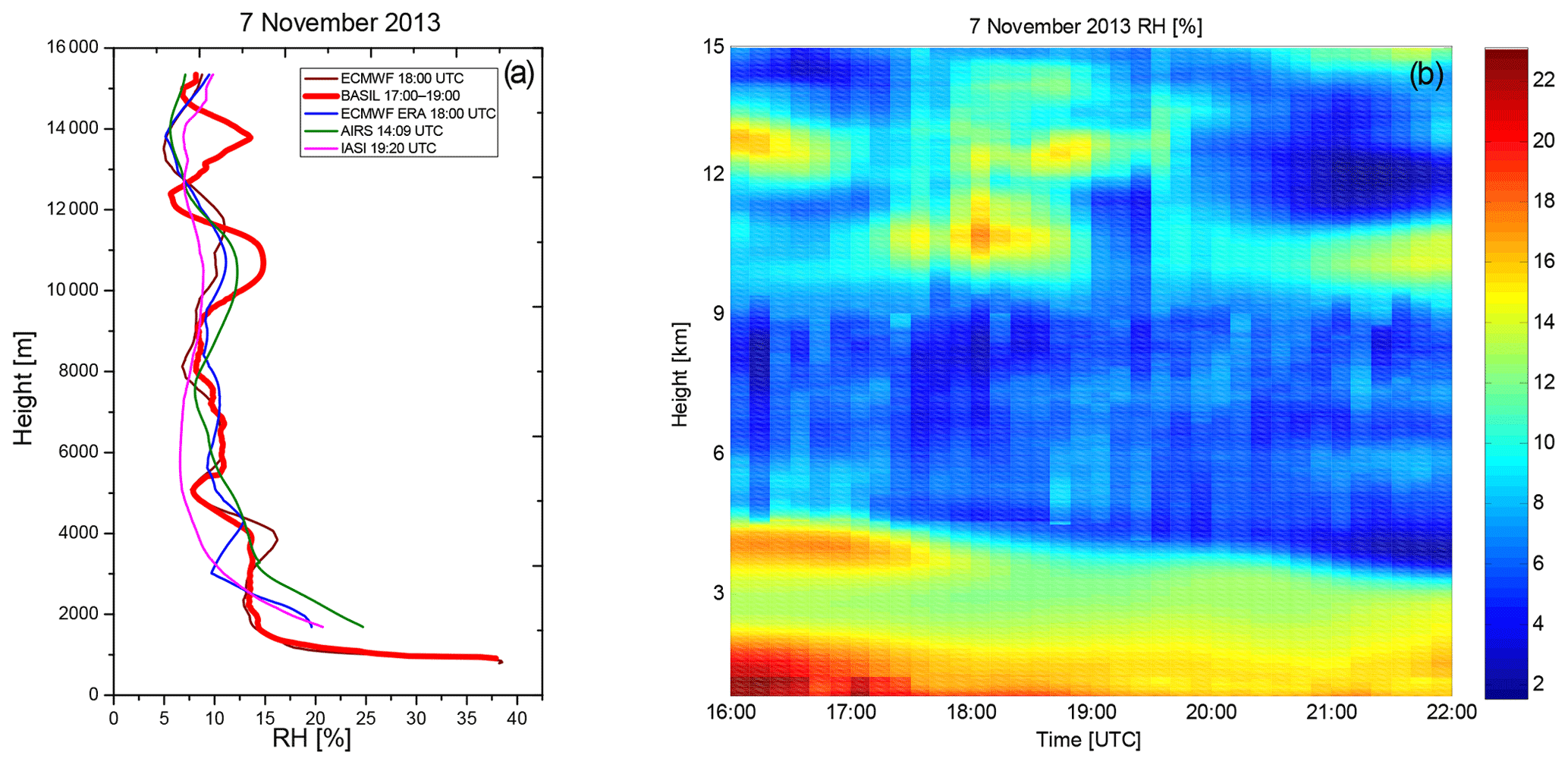
Figure 5 Vertical profile of relative humidity as measured by BASIL over the time period from 17:00 to 19:00 UTC on 7 November 2013 and the closest profiles (in time) from IASI (at 19:20 UTC), AIRS (at 14:09 UTC) and the ECMWF (ERA-15 and ERA-40, at 18:00 UTC) model reanalysis (b). Time evolution of the relative humidity profile as measured by BASIL over the interval from 18:00 to 22:00 UTC on 7 November 2013 (a).

Figure 4b shows the evolution of the atmospheric temperature profile over the same 6 h time interval considered in Fig. 3b. Again, the figure is a succession of 72 consecutive 5 min averaged profiles. In this case, for the purpose of obtaining sufficiently high signal statistics, a vertical resolution of 150 m was considered. It is to be noticed that, despite the short integration time, the strong signal intensities, in combination with favourable clear weather conditions, allow for an altitude of 50 km to be reached. The tropopause region and its fluctuations are clearly visible in the figure.

Accurate relative humidity (RH) measurements are of paramount importance to determine cloud and aerosol radiative properties and related microphysical processes. RH has been demonstrated to have a critical influence on aerosol climate forcing (Pilins et al., 1995). Aerosol hygroscopic growth at high relative humidity levels may significantly influence the aerosol direct effect on climate (Wulfmeyer and Feingold, 2000). As described in Sect. 4.3, RH profiles are obtained from the simultaneous and independent measurements of the water vapour mixing ratio and temperature profiles carried out by BASIL. Figure 5a illustrates the mean atmospheric relative humidity profile measured by BASIL on 7 November 2013 over the same time period considered in Figs. 3a and 4a. The agreement between BASIL and the different sensors/models is good, with deviations not exceeding 10 % up to 15 km.

Figure 5b shows the time evolution of relative humidity over the same 6 h interval considered in Figs. 3b and 4b, the present figure is again a succession of 72 consecutive 5 min averaged profiles with a vertical resolution of 150 m. It is to be noticed that, despite the short integration time, an altitude of 15 km is reached, with measurements revealing a RH variability in the UTLS region that is systematically larger than the random uncertainty affecting the Raman lidar measurements.

5.3 Assessment of the bias and RMS deviation between the different sensors/models

The performance of the different profiling sensors and models considered in the present study are assessed using a dedicated statistical analysis. Specifically, for each sensor/model pair and each case study, the relative bias and root-mean-square (RMS) deviation profiles are determined in terms of both the water vapour mixing ratio and temperature.

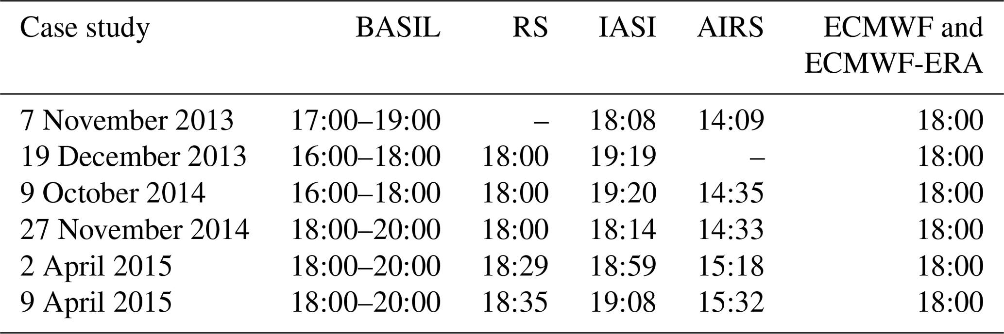
The overall number of all possible sensor/model pairs is 15, which is the maximum number of pairs possible when five sensors/models are available. More specifically, these are BASIL vs. radiosondes (RS), BASIL vs. IASI, BASIL vs. AIRS, BASIL vs. ECMWF, BASIL vs. ECMWF-ERA, RS vs. IASI, RS vs. AIRS, RS vs. ECMWF, RS vs. ECMWF-ERA, IASI vs. AIRS, IASI vs. ECMWF, IASI vs. ECMWF-ERA, AIRS vs. ECMWF, AIRS vs. ECMWF-ERA and ECMWF vs. ECMWF-ERA. The altitudinal intervals considered in the computation of the bias and RMS deviation profiles may vary for the different sensor/model pairs depending on the vertical coverage of the sensor considered, with the selection being driven by the sensor with lower coverage. In this regard, we have to recall that BASIL measurements of the water vapour mixing ratio and temperature profile extend up to 15 and 50 km respectively, whereas the radiosondes considered in the present study, which are those launched from the nearby IMAA-CNR station, provide profiles extending up to ∼30 km. Consequently, the altitudinal interval considered in the computation of the temperature bias and RMS deviation profiles is up to 30 km for those sensor/model pairs including the radiosondes, whereas is up to 50 km for all remaining sensor/model pairs. Conversely, the altitudinal interval considered in the computation of the water vapour mixing ratio bias and RMS deviation profiles is up to 15 km for all sensor/model pairs, owing to the lack of interest in water vapour profiles above the tropopause. For each sensor/model pair, we consider six comparisons, one for each of the case studies considered (7 November, 19 December 2013, 9 October, 27 November 2014, and 2 and 9 April 2015). The time interval considered is always the closest (in time) to the 2 h integration interval considered for the Raman lidar. Table 2 lists the time intervals for all sensors/models for all case studies considered.

Table 2 Time intervals for all sensors/models for all case studies considered.

For all intercomparisons reported in this paper, we computed bias and RMS deviation considering vertical intervals of 500 m (i.e. z₂–z₁ in Eqs. (14) and (15) is taken as equal to 500 m). Considering equally spaced data points with a vertical step of 30 m, the statistical analysis to compute the bias and RMS deviation is applied over 17 data points within each 500 m vertical interval.

Figure 6 shows the water vapour mixing ratio bias and RMS deviation profiles for all sensor/model pairs. As expected, the bias shows higher values in the ABL (in the range between −3 and +5 g kg⁻¹), with values typically being lower than ±1 g kg⁻¹ above 2 km. More specifically, in the ABL, the bias of BASIL vs. the radiosondes is in the range of ±0.3 g kg⁻¹, with similar small values also being observed in the comparison of BASIL with  ECMWF-ERA40. Higher bias values in the ABL are found to characterise the comparisons of BASIL/radisondes/ECMWF-ERA40 with IASI and AIRS, with values up to 5 g kg⁻¹. In this regard, it is to be pointed out that, while the distance between BASIL and the radiosonde launching facility (IMAA-CNR) is only ∼7 km and the grid point of ECMWF ERA-15 and ECMWF ERA-40 has a size of 9×9 km, is centred in between BASIL and IMAA-CNR, and includes both sites, the distance between the BASIL and IASI/AIRS footprint centres is ∼25 km, with these footprints being 12×12 km and 72×72 km respectively. Consequently, when comparing BASIL/radisondes/ECMWF-ERA40 with IASI and AIRS, the effects associated with water vapour heterogeneity are more important (see Fig. 1).

For all sensor/model pairs, the bias shows values lower than ±0.1 g kg⁻¹ above 8 km and lower than ±0.02 g kg⁻¹ above 10 km. In the altitudinal region from 8 to 16 km, the mutual bias of BASIL vs.  the radiosondes or ECMWF is lower than ±0.01 g kg⁻¹, whereas above 10 km the mutual bias of BASIL vs. ECMWF-ERA40 and AIRS vs. IASI is lower than ±0.07 g kg⁻¹. The mutual bias of BASIL vs. AIRS or IASI is lower than 0.01 g kg⁻¹ above 11 km. The RMS deviation values are comparable with bias values for all sensor/model pairs, which testifies to the fact that statistical uncertainties and changes in the measured/modelled atmospheric parameters poorly contribute to profiles' deviations. More specifically, for all sensor/model pairs, the RMS deviation shows values lower than ±1.5 g kg⁻¹ above 2 km, lower than ±0.1 g kg⁻¹ above 8 km and lower than ±0.02 g kg⁻¹ above 10 km.

For all sensor/model pairs, the percentage bias shows values in the range of ±60 % all the way up to 16 km. The smallest percentage bias is found in the comparison of BASIL with the radiosondes, with values not exceeding ±18 % all the way up to 12 km and values in the range of ±13 % above the ABL and up to 4 km. A small percentage bias is also found in the comparison of BASIL with ECMWF, with values not exceeding ±30 %. Positive percentage bias values in the range of 0 %–60 % are found to characterise the comparison of BASIL/radisondes/ECMWF-ERA40 with IASI and AIRS at all altitudes, which testifies to the fact that IASI and AIRS underestimate all other sensors/models. Percentage bias values in the range of ±25 % are found in the comparison of IASI with AIRS in the altitude region between 6 and 16 km, while higher values (up to 50 %) are found below 6 km; the agreement between the two sensors in the upper portion of the profile follows the fact that they both underestimate all of the other sensors/models considered (BASIL/radisondes/ECMWF-ERA). Values of the percentage RMS deviation for the comparison of BASIL with the radiosondes and ECMWF are lower than 40 % up to 11 km and lower than 30 % above. Values of the percentage RMS deviation that are typically lower than 50 %, but with sporadic values as large as 65 %–70 %, are found to characterise the comparison of BASIL/radiosondes/ECMWF-ERA with IASI and AIRS at all altitudes.

Figure 7 illustrates the temperature bias and RMS deviation profiles for all sensor/model pairs. The bias of BASIL vs. the radiosondes is in the range of ±1 K above the ABL up to 12 km, with deviations in the ABL not exceeding 2 K.

Except for a few points, bias values are within ±2 K up to 30 km, with this being the maximum altitude typically reached by the radiosondes. The bias of BASIL vs. ECMWF-ERA40 is within the range of ±0.8 K up to 12.5 km. For all sensor/model pairs, the bias shows values in the range of ±5 K all the way up to 50 km. As for the water vapour mixing ratio, RMS deviation values for all sensor/model pairs slightly exceed bias values, which testifies to the limited contribution of statistical uncertainties and changes in the measured/modelled atmospheric parameters in determining the deviations between profile pairs.

So far, we have reported and discussed the mutual bias and RMS deviation profiles between different sensors/models, highlighting the altitude variability of these quantities. However, in order to assess sensors' and models' performance, it is often preferable to use a single bias ∕ RMS deviation value. This leads us to the definition of the vertically averaged mean bias and the vertically averaged mean absolute bias.

The vertically averaged mean bias, $\stackrel{\mathrm{‾}}{\text{bias}}$, and RMS deviation, $\stackrel{\mathrm{‾}}{\text{RMS}}$, over the entire intercomparison range is determined via the application of the weighted mean (Bhawar et al., 2011):

$$\begin{array}{}\text{(17)}& \stackrel{\mathrm{‾}}{\text{bias}/\text{RMS}}={\displaystyle \frac{\sum _{i=\mathrm{1}}^M{w}_i\left({\text{bias}}_i/{\text{RMS}}_i\right)}{\sum _{i=\mathrm{1}}^M{w}_i}},\end{array}$$

where bias_i ∕ RMS_i is the mean bias ∕ RMS within the ith vertical interval, w_i is the corresponding weight and M is the number of vertical windows (each with a vertical extent of 500 m; see Sect. 4). M may vary for the different sensor/model pairs. For the comparisons in terms of the water vapour mixing ratio, which extend up to 15 km, the number of vertical windows N is equal to 30. The comparisons in terms of temperature extend up to 50 km for all of the different sensor/model pairs, with the number of vertical windows M being equal to 100; the only exceptions to this are comparisons including the radiosondes, as these profiles extend up to ∼30 km, and, in this case, the number of vertical windows M is typically equal to 60.

The weight w_i is given by the number of intercomparisons possible in the ith vertical window and varies between 0 (minimum weight) and 6 (maximum weight), this latter value representing the total number of case studies included in this intercomparisons effort. A weighted mean is necessary because the number of intercomparisons may be smaller when data are missing at some specific altitudes; thus, data from these altitudes must have a lower weight in the vertically averaged mean. The use of a weighted mean is particularly important in intercomparison efforts where the vertical coverage of the sensors/models compared may vary from one case study to the next.

The vertically averaged absolute mean bias, $\stackrel{\mathrm{‾}}{\left|\text{bias}\right|}$, and the RMS deviation, $\stackrel{\mathrm{‾}}{\left|\text{RMS}\right|}$, defined as the weighted mean of the moduli of the single bias values at different altitudes, can be determined via the following expression:

$$\begin{array}{}\text{(18)}& \stackrel{\mathrm{‾}}{\left|\text{bias/RMS}\right|}={\displaystyle \frac{\sum _{i=\mathrm{1}}^M{w}_i\left|{\text{bias}}_i/{\text{RMS}}_i\right|}{\sum _{i=\mathrm{1}}^N{w}_i}}.\end{array}$$

In the vertically averaged absolute mean bias, $\stackrel{\mathrm{‾}}{\left|\text{bias}\right|}$, values at different altitudes with different signs will not cancel out. Consequently, values of $\stackrel{\mathrm{‾}}{\left|\text{bias}\right|}$ are higher than the corresponding $\stackrel{\mathrm{‾}}{\text{bias}}$ values.

Figure 6 Vertical profiles of the water vapour mixing ratio mean bias and RMS deviation for all sensor/model pairs: bias (a), RMS (b), percentage bias (c) and percentage RMS (d).

Table 3 includes the vertically averaged mean mutual bias, $\stackrel{\mathrm{‾}}{\text{bias}}$, and RMS deviation, $\stackrel{\mathrm{‾}}{\text{RMS}}$, values and the vertically averaged absolute mean mutual bias values, $\stackrel{\mathrm{‾}}{\left|\text{bias}\right|}$, for the water vapour mixing ratio intercomparison, which includes all possible sensor/model pairs. The lowest $\stackrel{\mathrm{‾}}{\text{bias}}$ value is found to characterise the comparison of radiosondes with BASIL (0.025 g kg⁻¹). Low values of $\stackrel{\mathrm{‾}}{\text{bias}}$ are also found in the comparison of ECMWF and ECMWF-ERA40 with IASI and AIRS (ECMWF vs. IASI = −0.0295 g kg⁻¹, ECMWF vs. AIRS = −0.042 g kg⁻¹, ECMWF-ERA40 vs. IASI = 0.053 kg⁻¹ and ECMWF-ERA40 vs. AIRS = 0.086 g kg⁻¹). As a possible reason for these low values, it should be considered that ECMWF reanalysis products, such as those used in the present intercomparison effort (ECMWF ERA-15 and ERA-40), heavily rely on the assimilation of IASI and AIRS data, especially in the UTLS region. This aspect is also responsible for the low $\stackrel{\mathrm{‾}}{\text{bias}}$ value of ECMWF vs. ECMWF ERA (−0.056 g kg⁻¹). Higher $\stackrel{\mathrm{‾}}{\text{bias}}$ values are found to characterise the comparison of BASIL/radiosondes with IASI, AIRS, ECMWF and ECMWF-ERA40. With respect to the vertically averaged absolute mean bias, $\stackrel{\mathrm{‾}}{\left|\text{bias}\right|}$, values are somewhat higher than those of the $\stackrel{\mathrm{‾}}{\text{bias}}$. Specifically, the value of $\stackrel{\mathrm{‾}}{\left|\text{bias}\right|}$ for the comparison of radiosondes with BASIL is 0.05 g kg⁻¹. Relatively small values of $\stackrel{\mathrm{‾}}{\left|\text{bias}\right|}$ are also found in the comparison of ECMWF and ECMWF-ERA40 with IASI and AIRS (ECMWF vs. IASI = 0.16 g kg⁻¹, ECMWF vs. AIRS = 0.29 g kg⁻¹, ECMWF-ERA40 vs. IASI = 0.41 kg⁻¹ and ECMWF-ERA40 vs. AIRS = 0.27 g kg⁻¹).

The value of $\stackrel{\mathrm{‾}}{\text{RMS}}$ for the comparison of radiosondes with BASIL is 0.135 g kg⁻¹, which is significantly higher than the corresponding $\stackrel{\mathrm{‾}}{\text{bias}}$ values. This is most probably owing to the large statistical uncertainty affecting BASIL measurements in the UTLS region and the radiosonde horizontal drift, which determines humidity profile variations that are associated with different sounded air masses. High $\stackrel{\mathrm{‾}}{\text{RMS}}$ values are also found to characterise the comparison of AIRS with all other sensors/models (AIRS vs. BASIL = 0.446 g kg⁻¹, AIRS vs. CNR = 0.687 g kg⁻¹, AIRS vs. IASI = 0.381 g kg⁻¹, AIRS vs. ECMWF = 0.33 g kg⁻¹ and AIRS vs. ECMWF-ERA40 = 0.216 g kg⁻¹). The reason for these large values is the large size of the AIRS footprint (72×72 km), which results in a measurement loss of representativeness when compared with all other localised sensor/model data. Large values of $\stackrel{\mathrm{‾}}{\text{RMS}}$ are also found to characterise the comparison of IASI with all other sensors/models (IASI vs.  BASIL = 0.302 g kg⁻¹, IASI vs. RS = 0.63 g kg⁻¹, IASI vs. ECMWF = 0.165 g kg⁻¹ and IASI vs. ECMWF-ERA40 = 0.252 g kg⁻¹). Such large values are possibly associated with the considerable distance between the IASI footprint and all other sensors and models, especially in the presence of horizontal heterogeneities in the humidity field. The high $\stackrel{\mathrm{‾}}{\text{RMS}}$ values characterising the comparisons of BASIL/radiosondes with ECMWF/ECMWF-ERA40 are again possibly associated with the limited effectiveness of these reanalyses within the ABL, where most humidity is located, as well as with their poor effectiveness in the UTLS region.

Table 3 Water vapour mixing ratio vertically averaged mean and absolute mean bias and the RMS deviation values for all of the sensor/model pairs considered.

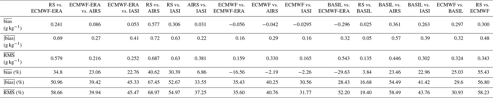
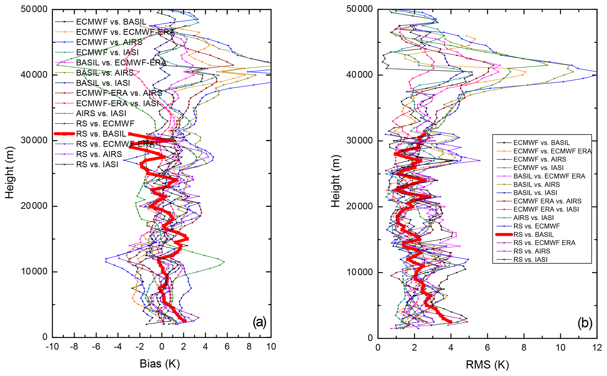
Figure 7 Vertical profiles of the temperature mean bias and RMS deviation for all sensor/model pairs: (a) bias and (b) RMS .

Values of the percentage $\stackrel{\mathrm{‾}}{\text{bias}}$ confirm most of the considerations above. It is to be pointed out that the percentage $\stackrel{\mathrm{‾}}{\text{bias}}$ is a quantity very sensitive to the variability of water vapour mixing ratio values in the UTLS region, more than the $\stackrel{\mathrm{‾}}{\text{bias}}$, as the water vapour mixing ratio actually has a large variability within the troposphere, varying over 4 orders of magnitude from the surface to the UTLS region. A very small percentage $\stackrel{\mathrm{‾}}{\text{bias}}$ value is found to characterise the comparison of radiosondes with BASIL (3.84 %), testifying to the accuracy and agreement of these two sensors throughout the sounded vertical interval, especially in the ABL and UTLS. Low percentage $\stackrel{\mathrm{‾}}{\text{bias}}$ values are also found to characterise the comparison of ECMWF with IASI/AIRS (ECMWF vs. IASI = −2.26 % and ECMWF vs. AIRS = −2.19 %). Relatively low $\stackrel{\mathrm{‾}}{\left|\text{bias}\right|}$ values are also found to characterise the comparison of radiosondes with BASIL (16.7 %) and the comparison of ECMWF with IASI/AIRS (ECMWF vs. IASI = 30.56 % and ECMWF vs. AIRS = 29.6 %).

Figure 8 Overall bias affecting the water vapour profile (a) and temperature (b) data.

Table 4 includes the vertically averaged mean mutual bias and RMS deviation values, $\stackrel{\mathrm{‾}}{\text{bias}}$ and $\stackrel{\mathrm{‾}}{\text{RMS}}$, and the vertically averaged absolute mean mutual bias values, $\stackrel{\mathrm{‾}}{\left|\text{bias}\right|}$, for the temperature intercomparison for all sensor/model pairs considered. It is to be specified that, while an estimate of the percentage bias and RMS deviation is necessary for the adequate assessment of the quality (accuracy/precision) of the water vapour mixing ratio measurements/analyses, as these quantities may vary by more than 4 orders of magnitude in the altitudinal interval considered in this intercomparison effort (0–16 km), there is no need for an estimate of the percentage bias and RMS deviation characterising temperature measurements/analyses; this is due to the fact that the latter quantities are characterised by a much lower variability (not exceeding 30 %) in the interval considered (0–50 km), with the highest values at the surface (typically 280–300 K) and the lowest values at the tropopause (typically 200–210 K). The lowest $\stackrel{\mathrm{‾}}{\text{bias}}$ values characterise the comparison of radiosondes with BASIL (0.03 K) and ECMWF-ERA40 with IASI (−0.14 K). Low $\stackrel{\mathrm{‾}}{\text{bias}}$ values are also found in the comparison of ECMWF with BASIL (−0.14 K), BASIL with ECMWF-ERA40 (0.43 K), BASIL with IASI (0.21 K), RS with ECMWF (0.57 K), ECMWF-ERA40 with RS (0.28 K) and RS with IASI (0.51 K). Low $\stackrel{\mathrm{‾}}{\text{bias}}$ values are also found to characterise the comparison of ECMWF with ECMWF-ERA40 (0.58 K) and ECMWF with IASI (0.65 K). Higher $\stackrel{\mathrm{‾}}{\text{bias}}$ values are found to characterise the comparison of AIRS with all other sensors/models (BASIL vs. AIRS = 1.95 K, RS vs. AIRS = 0.89, AIRS vs. IASI = −1.33 K, ECMWF vs. AIRS = 2.14 K and ECMWF-ERA40 vs. AIRS = 1.19 K), with AIRS always underestimating all of the other sensors and models. The above results reveal, with the exception of AIRS, very good agreement between all sensors and a remarkable capability for the models considered to reproduce the measured temperature profiles. As clearly shown by the bias profiles in Fig. 7a, most of the bias between AIRS and all of the other sensors/models is found above 37 km, which reveals a negative systematic uncertainty affecting AIRS temperature profile measurements above this altitude (AIRS underestimates all other sensors/models) up to 5 K. Part of this bias is also attributed to the fact that AIRS slightly underestimates all of the other sensors/models around the tropopause. Additionally, the small bias characterising the comparisons of IASI with all other sensors/models testify to the very good performance of this sensor in terms of temperature profile measurements and its correct assimilation in ECMWF analyses. With a few exceptions, values of $\stackrel{\mathrm{‾}}{\left|\text{bias}\right|}$ are in the range of 1–2 K. A low $\stackrel{\mathrm{‾}}{\text{RMS}}$ deviation value characterises the comparison of BASIL with the radiosondes (1.86 K). This low value is attributed to the fact that the comparison between BASIL and the radiosondes only extends up to 30 km; consequently, the effects associated with the large statistical fluctuations affecting BASIL signals in the 30–50 km region, with the sounding of different air masses and with gravity wave propagation, are significantly reduced. Relatively small $\stackrel{\mathrm{‾}}{\text{RMS}}$ values are also found in the comparison of ECMWF/ECMWF-ERA40 with IASI (1.88 and 1.83 K respectively).

Table 4 Temperature vertically averaged mean and absolute mean bias and RMS deviation values for all considered sensor/model pairs.

5.4 Overall bias affecting all sensors/models

Making use of the available statistics of comparison results, an approach is considered to determine the overall bias values for all sensors/models involved in this intercomparison effort. This approach, originally proposed by Behrendt et al. (2007a, b), can be applied when there is at least one sensor whose measurements are comparable with all other sensors/models. For this purpose we considered the BASIL Raman lidar. Assuming equal weight on the data reliability of each sensor/model, an estimate of the overall bias affecting all sensors/models is obtained by imposing the condition that the summation of all mutual biases between the sensor/model pairs is equal to zero. The choice of attributing equal weight to the data reliability of each sensor/model is driven by the awareness that none of them can be assumed a priori to be more accurate than the others and, thus, by the assumption that the closest profile to a reference profile can be obtained by taking the mean of all of the available profiles. Based on this approach, the overall bias affecting the water vapour profile data from BASIL, the radiosondes, IASI, AIRS, ECMWF and ECMWF-ERA40 is estimated to be −0.04, 0.20, −0.31, −0.40, 0.25 and 0.25 g kg⁻¹ respectively, as shown in Fig. 8a.

The same approach was applied to determine the overall bias for temperature profile data from all of the sensors/models involved in this intercomparison effort. In this case, as we have previously identified a significant systematic uncertainty affecting AIRS measurements, this sensor was excluded from the summation of all mutual biases between sensor/model pairs. Thus, assuming equal weight on the data reliability of all of the other sensors/models, the overall bias affecting temperature profile data from BASIL, the radiosondes, IASI, AIRS, ECMWF and ECMWF-ERA40 is found to be 0.19, 0.22, −0.02, −1.76, 0.04 and −0.24 K respectively, as shown in Fig. 8b.

6 Summary

Case studies illustrated in this paper demonstrate the ability of BASIL to perform temperature profile measurements up to 50 km and water vapour mixing ratio profile measurements up to 15 km, considering an integration time of 2 h and a vertical resolution of 150–600 m, with a measurement accuracy of 0.1 K and 0.1 g kg⁻¹ respectively. Temperature and water vapour profile measurements carried out by BASIL are compared with profiles from a variety of other sensors/models, namely radiosondes, the IASI and AIRS satellite instruments, and model reanalyses data (ECMWF and ECMWF-ERA). Comparisons between BASIL and the different sensor/model data in terms of the water vapour mixing ratio indicate a vertically averaged mean mutual bias of −0.026 g kg⁻¹ (or −3.8 %), 0.263 g kg⁻¹ (or 30.0 %), 0.361 g kg⁻¹ (or 23.5 %), −0.297 g kg⁻¹ (or −25 %) and −0.296 g kg⁻¹ (or −29.6 %), when compared with radiosondes, IASI, AIRS, ECMWF and ECMWF-ERA respectively. The vertically averaged absolute mean mutual biases are somewhat higher, i.e. 0.05 g kg⁻¹ (or 16.7 %), 0.39 g kg⁻¹ (or 23.0 %), 0.57 g kg⁻¹(or 23.5 %), 0.32 g kg⁻¹ (or 29.6 %) and 0.52 g kg⁻¹ (or 53.3 %), when comparing BASIL with radiosondes, IASI, AIRS, ECMWF and ECMWF-ERA respectively. Comparisons in terms of the temperature measurements reveal a mean/absolute mean mutual bias between BASIL and the radiosondes, IASI, AIRS, ECMWF and ECMWF-ERA of $-\mathrm{0.03}/\mathrm{1.28}$, 0.21∕1.30, 1.95∕3.50, 0.14∕1.76 and 0.43∕1.63 K respectively. Higher temperature biases are found between AIRS and all of the other sensors/models, which is the result of AIRS slightly underestimating all of the other sensors/models around the tropopause and above 37 km.

The possibility of assessing the overall bias values for all of the sensors/models included in this intercomparison effort was also exploited, benefiting from the circumstance that the BASIL Raman lidar could be compared with all other sensor/model data. The overall bias affecting water vapour/temperature profile data from BASIL, the radiosondes, IASI, AIRS, ECMWF and ECMWF-ERA40 was estimated to be −0.04 g kg${}^{-\mathrm{1}}/\mathrm{0.19}$ K, 0.20 g kg${}^{-\mathrm{1}}/\mathrm{0.22}$ K, −0.31 g kg${}^{-\mathrm{1}}/-\mathrm{0.02}$ K, −0.40 g kg${}^{-\mathrm{1}}/-\mathrm{1.76}$ K, 0.25 g kg${}^{-\mathrm{1}}/\mathrm{0.04}$ K and 0.25 g kg${}^{-\mathrm{1}}/-\mathrm{0.24}$ K respectively.

The present study allows us to gain confidence in the high quality of the water vapour and temperature profiling carried out by BASIL and included in the NDACC database as well as in the possibility of using long-term records of these measurements for monitoring atmospheric composition and thermal structure changes and, ultimately, for climate trend studies.