the Creative Commons Attribution 4.0 License.
the Creative Commons Attribution 4.0 License.
 | 29 Jul 2020
Capturing temporal heterogeneity in soil nitrous oxide fluxes with a robust and low-cost automated chamber apparatus
Nathaniel C. Lawrence
Soils play an important role in Earth's climate system through their regulation of trace greenhouse gases. Despite decades of soil gas flux measurements using manual chamber methods, limited temporal coverage has led to high uncertainty in flux magnitude and variability, particularly during peak emission events. Automated chamber measurement systems can collect high-frequency (subdaily) measurements across various spatial scales but may be prohibitively expensive or incompatible with field conditions. Here we describe the construction and operational details for a robust, relatively inexpensive, and adaptable automated dynamic (steady-state) chamber measurement system modified from previously published methods, using relatively low cost analyzers to measure nitrous oxide (N2O) and carbon dioxide (CO2). The system was robust to intermittent flooding of chambers, long tubing runs (>100 m), and operational temperature extremes (−12 to 39 ∘C) and was entirely powered by solar energy. Using data collected between 2017 and 2019 we tested the underlying principles of chamber operation and examined N2O diel variation and rain-pulse timing that would be difficult to characterize using infrequent manual measurements. Stable steady-state flux dynamics were achieved during 29 min chamber closure periods at a relatively low flow rate (2 L min−1). Instrument performance and calculated fluxes were minimally impacted by variation in air temperature and water vapor. Measurements between 08:00 and 12:00 LT were closest to the daily mean N2O and CO2 emission. Afternoon fluxes (12:00–16:00 LT) were 28 % higher than the daily mean for N2O (4.04 vs. 3.15 nmol m−2 s−1) and were 22 % higher for CO2 (4.38 vs. 3.60 ). High rates of N2O emission are frequently observed after precipitation. Following four discrete rainfall events, we found a 12–26 h delay before peak N2O flux, which would be difficult to capture with manual measurements. Our observation of substantial and variable diel trends and rapid but variable onset of high N2O emissions following rainfall supports the need for high-frequency measurements.
- Article
(1866 KB) - Full-text XML
-
Supplement
(227 KB) - BibTeX
- EndNote


Soils play a critical role in Earth's carbon (C) and nitrogen (N) cycles. Managing soils to sequester C or reduce the emission of the trace greenhouse gases N2O and methane (CH4) is often suggested as an effective tool to combat climate change (Minasny et al., 2017; Paustian et al., 2016). Therefore, reliable trace gas measurements are critical for informing management. Although manual soil gas flux measurements have been collected for several decades, the high temporal and spatial variability of emissions has often plagued attempts to obtain accurate and precise flux estimates needed to calculate annual budgets (Davidson et al., 2002; Groffman et al., 2009; Hutchinson and Mosier, 1981). Sampling at higher frequency than is practical with manual measurements may be required to constrain the role of soils in global biogeochemical cycles and validate the impacts of management practices on trace gas emissions (Barton et al., 2015; Merbold et al., 2015; Parkin, 2008). N2O emissions are particularly variable, so relatively less is known about peak emissions such as the time between rainfall and the subsequent N2O pulse that is frequently observed (Groffman et al., 2006, 2009). High-frequency automated flux measurements that can span the large (>100 m) spatial scales that frequently accompany local topographical and hydrological variation at a site may be critical to capture the dual spatial–temporal dynamics which are key to generating robust emission estimates.
Prefabricated automated chambers capable of measuring soil trace gas fluxes are available commercially and can be plumbed to a wide range of analyzers – most commonly, infrared gas analyzers that measure CO2. Commercially available chambers typically rely on electric components for movement which are sensitive to moisture, and they are substantially more expensive (often many thousands of US dollars, USD) than the chamber design described here (materials costs of ∼ USD 500 per chamber). Other custom-built chamber designs have been developed to address specific research needs (e.g., Ambus and Robertson, 1998; Butterbach-Bahl et al., 1997; Savage et al., 2014). Chambers have been paired with analyzers to measure other trace gases, including N2O and CH4, by utilizing methods such as gas chromatography (GC), photoacoustic infrared detection, tunable diode laser (TDL), or cavity ring-down laser spectroscopy (Ambus and Robertson, 1998; Breuer et al., 2000; Courtois et al., 2019; Papen and Butterbach-Bahl, 1999; Pihlatie et al., 2005). Fassbinder et al. (2013) provide a detailed summary of the advantages and limitations of commonly used analyzers that we briefly summarize here. GC systems with electron capture detectors (ECDs) have often been used to measure N2O from automated chambers (Breuer et al., 2000; Papen and Butterbach-Bahl, 1999). However, GC systems typically have high power demand and require carrier gases and radioactive elements for ECD operation that may limit their field practicality. Interference from water vapor and other gases potentially limits the use of photoacoustic analyzers in the field (Rosenstock et al., 2013). Laser-based analytical approaches are capable of rapid (e.g., 10 Hz) and precise N2O measurements, but these analyzers are considerably more expensive (> USD 70 000) and often have relatively high power requirements for autonomous field deployment (Fassbinder et al., 2013; Pihlatie et al., 2005). We sought to implement a lower-cost, solar-powered, soil gas flux measurement system capable of operating unattended in a harsh field environment and where analyzers could feasibly be replaced if stolen or damaged. For these reasons, we utilized a gas filter correlation (GFC) infrared N2O analyzer in our study (∼ USD 16 000), similar to that described previously by Fassbinder et al. (2013), along with an infrared gas analyzer for CO2 and H2O measurement (∼ USD 4000). However, other analyzers could be readily employed with the chamber and manifold system described below.
Environmental conditions, particularly those posed by flooding and agricultural management, created several unique challenges for trace gas measurement in our study system that could be expected in many field settings. Extreme heat and cold (−12 to 39 ∘C) and occasional submergence of chambers mandated that our apparatus be tolerant of a wide range of conditions. Frequent agricultural management (tillage, planting, fertilization, harvest, etc.) at our field site required the chambers and associated equipment to be relatively portable so they could be removed to the field edge (∼100 m away) and reinstalled several times per year (Fig. 1a). To avoid damaging crops, all equipment had to be movable on foot. Because electric power was unavailable, solar panels and batteries had to provide all necessary energy. Our core measurement system consisted of eight steady-state, flow-through chambers that quantified soil gas fluxes at each chamber every 4 h. For 1 year, a second set of chambers was paired with the original 8 for a total of 16 chambers without sacrificing measurement frequency. With our design, chamber number and measurement frequency can be readily adjusted to fit study questions. The gas analyzers were maintained in an instrument shed at the field edge (Fig. 1a). This location was not impacted by flooding or agricultural management but was subjected to the temperature extremes noted above.
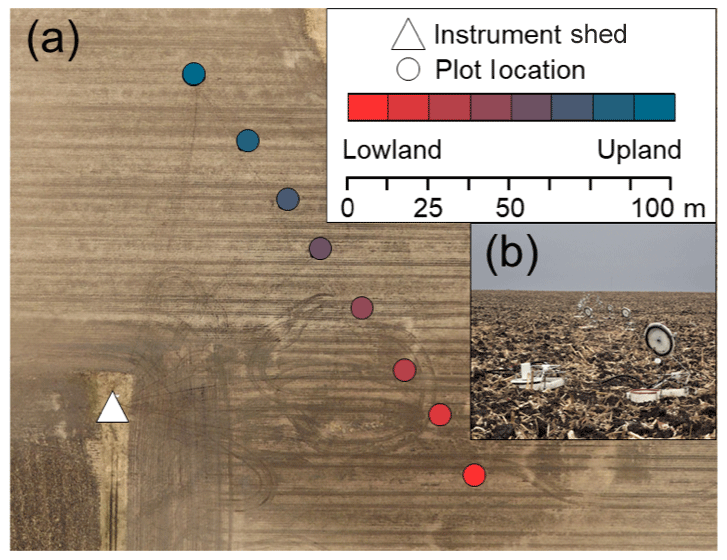
Figure 1(a) Aerial image of the field site with plot locations. (b) Image from the lowest topographic position along the transect (front left: a closed chamber; front right: an open chamber between measurements); the transect is visible in the background. Aerial image source: Esri, DigitalGlobe, GeoEye, Earthstar Geographics, CNES/Airbus DS, USDA, USGS, AeroGRID, IGN, and the GIS user community.
There is a rich literature on the impacts of chamber design and the potential biases of soil trace gas flux measurements. We chose a chamber design that has been shown in field and laboratory experiments to provide accurate estimation of soil gas fluxes and isotopic composition (Bowling et al., 2015; Moyes et al., 2010a; Norman et al., 1997; Pumpanen et al., 2004). In one comparison of different chambers, a variant of the open, flow-through design we used here measured known CO2 fluxes produced in the laboratory to within 2 %–4 % of the actual values, which was relatively accurate compared to the other designs tested (Pumpanen et al., 2004). Pressure differential between the inside and outside of some chamber designs can create measurement artifacts (Fang and Moncrieff, 1998; Xu et al., 2006). The chambers described here utilize an open-lid design (Fig. 2) that limits pressure differential to less than −0.2 Pa at the flow rate (2 L min−1) we utilized (Moyes et al., 2010b; Rayment and Jarvis, 1997). When using static chamber designs, soil gas flux is calculated as a function of the change in gas concentration over time within a closed chamber headspace. In contrast, with dynamic chambers we derive gas flux from the steady-state difference in concentration between air at the chamber inlet and air pumped out of a chamber outlet (Fig. 2). When the outlet gas concentration is approximately constant, the chamber is at a steady state. Steady-state chambers with low pressure differential have been shown to reproduce known δ13C values of CO2 fluxes (Moyes et al., 2010b), possibly because they have less impact on the diffusive profile than many non-steady-state chamber designs (Nickerson and Risk, 2009). For our study, an additional consideration was that chambers needed to be located at variable distances (80–115 m) from the gas analyzers (Fig. 1a). We required this attribute to span a large (120 m) topographic gradient and to maintain analyzers and related instruments in a permanent location with vehicle access. As sampled gas can be vented downstream of the analyzers instead of routed back to the chamber (as is required for closed-loop static chamber designs), dynamic chambers can be located at varying distances from the instruments without impacting the effective volume of the chamber headspace.
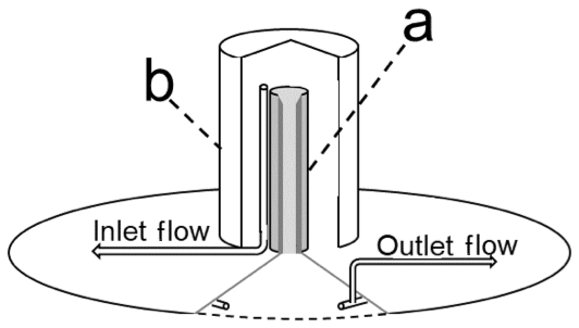
Figure 2Illustration modified from Rayment and Jarvis (1997) depicting the chamber lid with cutout to show the inlet tube (a) and the polyvinyl chloride (PVC) cap (b). Inlet and outlet sampling points are noted.
In this publication we present a method to construct a robust system of dynamic automated soil trace gas chambers along with the maintenance and troubleshooting lessons learned over the 3-year period the chambers were running. In addition to presenting these operational details, we tested three underlying assumptions of our chamber design: (1) did chambers reach steady-state dynamics, (2) how did broad temperature fluctuations affect instrument performance in the field, and (3) to what extent could water vapor impact our measurement values? We further utilized the high-frequency flux data to test two questions related to the temporal dynamics of gas emissions to inform manual sampling efforts: (4) how strong was the diel signal in trace gas emissions and (5) what was the average delay between isolated rainfall events and the elevated N2O emissions that frequently followed?
2.1 Study site
Our chambers were located at eight plots on 17 m intervals along a topographic gradient in a conventionally managed corn–soybean (Zea mays–Glycine max) agricultural field in central Iowa, USA (41.98∘ N, 93.69∘ W). The transect spanned a distance of 120 m (Fig. 1a), 2.25 m elevation, and included very poorly to moderately poorly drained soils (Mollisols classified as Okoboji to Clarion series under the US Department of Agriculture taxonomy). Chambers were placed immediately adjacent to crop plants; due to frequent tillage and herbicide application, recruitment of other plants inside the chamber collars was uncommon, but any plants were removed from the chamber interiors as soon as they were observed. Roots from crop plants were not excluded and likely grew beneath chambers. The lower half of the transect often experienced flooding after large rain events (Logsdon and James, 2014), and chambers were occasionally completely inundated. The foreground of Fig. 1b shows one open and one closed chamber located in the lowest topographic position. The open chambers in the background are positioned along the topographic transect.
2.2 Chamber design
The chambers we utilized were constructed in-house, and various aspects were modified from previously published methods. The chamber lid was first described by Rayment and Jarvis (1997), and Riggs et al. (2009) pioneered a pneumatic piston and stainless-steel frame that opened and closed a chamber lid relative to a collar installed in the soil. Bowling et al. (2015) implemented a similar chamber design to measure CO2 and δ13C fluxes from a forest but did not include extensive details on chamber design, construction, or operation.
The dimensions of many of the materials used were commercially specified with imperial units but are reported here in metric equivalents for consistency. A table providing the instrument part names in the order that they are described, along with use, supplier, part number, and total cost, is supplied in the Supplement. Small, unspecified items (e.g., bolts) which do not require exact dimensions are not listed. Approximately 130–260 h of labor was required to construct nine chambers and assemble the associated control system. Figure 3 shows the chamber design. Here we define the chamber base as the rigid, rectangular polyethylene structure (Fig. 3a) and the chamber frame as the metal structure superior to the base which allows for movement of the chamber lid (Fig. 3). The chamber collar is defined as the length of polyvinyl chloride (PVC) pipe that forms the interface between the chamber lid and the soil. Chamber bases were constructed from 2.54 cm×7.62 cm high-density polyethylene (HDPE) plastic (Fig. 3a). Custom L brackets cut from 5.08 cm aluminum angle stock and bolted to the plastic base provided two horizontal platforms to attach female spherical rod ends that served as the pivot point for opening and closing the chamber (Fig. 3b). By routing vertical slots in the L brackets, we provided a means to adjust the lateral orientation of the pivot rod on each chamber after installation in the field (Fig. 3b). This was useful to ensure that the chamber lid sealed against the collar given the inherent variability of soil microtopography. A 0.64 cm diameter threaded rod between the rod ends provided an axle to attach the chamber frame (Fig. 3c). Most of the chamber frame was constructed from 0.95 cm diameter stainless-steel tubing; dimensions are listed in the caption and correspond to the numbered labels in Fig. 3. To drill holes in the stainless-steel tubing, we flattened the ends of each piece of tubing to a length of 1 cm in a bench vise and then drilled holes through the flattened portion to accommodate attachment bolts. The stainless-steel tubing was attached to the threaded rod described above or to aluminum angle brackets bolted to the chamber lid, noted by yellow or red circles respectively in Fig. 3. Two lengths of 1.27 cm diameter stainless-steel tubing surrounding a second 0.64 cm diameter threaded rod and inserted into a 5.08 cm×2.54 cm HDPE bar with a slot for a spherical rod end were attached to the end of a pneumatic cylinder rod piston (Clippard, UDR-17-6) (Fig. 3d). Extension of the piston moved the chamber lid open or closed, and the HDPE bar and stainless-steel tubing were used to prevent the threaded rod from flexing during movement of the chamber lid. The three spherical rod ends, two located on the pivot point and one at the end of the cylinder piston, served as rotational degrees of motion (Fig. 3, yellow circles). All other connection points were rigid (Fig. 3, red circles).
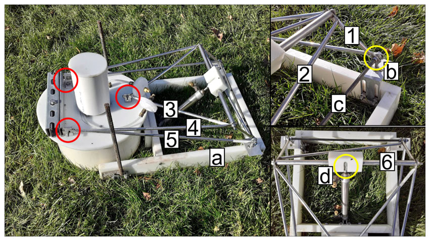
Figure 3Image of chamber design: HDPE base (a), aluminum L bracket (b), threaded rod (c), and pneumatic cylinder rod end (d). The length of each numbered stainless-steel tube is as follows: 1 (16 cm), 2 (47 cm), 3 (41 cm), 4 (56 cm), 5 (65 cm), and 6 (18 cm). The yellow circles indicate points of rotation while red circles denote rigid, fixed connection points.
The chamber lid followed a previous design which was shown to minimize the pressure differential between the inside and outside of the chamber (<0.2 Pa at flow rates of 4.5 L min−1) (Moyes et al., 2010b; Rayment and Jarvis, 1997). The circular chamber lid (38 cm diameter) was cut from an HDPE panel (1.27 cm thick). A 2.54 cm diameter hole cut into the center of the lid allowed a vertical gas inlet tube (Fig. 2a) to be fixed to the lid via custom-machined threads and a nut on the bottom of the tube. The inlet tube (15 cm length) was machined from aluminum bar stock and had internal and external diameters of 2.54 and 3.81 cm, respectively, and a taper (2.54 cm length) at the superior end (Fig. 2a). The inlet tube was covered by a PVC cap (10.16 cm diameter and 16 cm length; Fig. 2b) attached to the lid surface with three bolts, each with 1 cm spacers to create an air gap between the cap and the lid surface (Fig. 2). The gap created by the spacers allowed air to flow to the inlet while preventing the direct horizontal flow of wind over the inlet tube opening. On the lower surface of the lid, a D-shaped rubber seal (EPDM foam, 2.54 cm width) was affixed with silicone caulk in a ring where the lid contacted the collar to create an airtight seal when pressure was applied to the piston that closed the chamber (Fig. 1b). Early in our study, we observed that high pressure (>550 kPa) was needed to ensure a tight seal between the collar and chamber lid. To minimize the piston air pressure required to seal the chamber lid against the collar, and thus conserve power, we bolted two nested, 26 cm sections of slotted steel construction strut to the top of the chamber lid to provide additional mass (Fig. 3). Gas from the inside of the chamber was sampled via a circular outlet manifold consisting of polyethylene tubing (6.4 mm o.d., 3.2 mm i.d.) perforated by drilling 2 mm diameter holes through the tubing at 2 cm intervals, and it was held in place approximately 3 cm below the lower surface of the lid with three stainless-steel eyebolts. All tubing connections in our chamber and instrument manifolds were made using 0.64 cm brass Swagelok compression fittings. A threaded bulkhead union and tee fitting were used to connect to the outlet manifold to external tubing above the chamber lid.
Chamber collars were made from PVC pipe segments (20 cm length, 30.48 cm i.d.) with the lower edge beveled with a belt sander to facilitate insertion into the soil. The beveled edge was pounded 10 cm into the soil for a total collar height of 10 cm and volume of approximately 7.3 L. The volume of air inside the longest length of tubing (120 m) connecting the chamber lid to the gas analyzers was <1.8 L. To hold the chamber base in place relative to the collar, we initially used a ratchet strap. However, we found that pressure exerted by the pneumatic arm when opening or closing the chamber occasionally shifted the position of the chamber base or collar and prevented a seal between the chamber lid, collar, and soil. This occasionally occurred following tillage or when soils were extremely dry, given that these soils contained swelling clays. To address this problem, we anchored the chamber base using two steel rebar rods (60 cm length, 1.27 cm diameter) pounded 45 cm into the ground on either side of the chamber base and affixed to the outside of the chamber base with U bolts positioned along the central axis of the collar (Fig. 3). We periodically checked that the chamber lids were effectively sealing against the collars. Application of this method to true Vertisols, with even greater shrink/swell behavior, could likely be achieved using similar use of rebar to anchor the chamber.
2.3 Chamber lid operation
Chambers were opened and sealed by alternatively applying 550 kPa pressurized air to either side of the pneumatic cylinder described above via two lengths of tubing connecting each chamber and the instrument shed (Fig. 4a). We used 0.64 cm o.d., 0.43 cm i.d. low-density polyethylene (LDPE) plastic tubing. We initially used aluminum composite tubing (Synflex 1300), which has been commonly used in other field trace gas measurement studies (e.g., Bowling et al., 2015), but we found this to be impractical for our application given its vulnerability to kinking during chamber installation and removal through dense vegetation. Pressurized gas tubing was connected to the pneumatic cylinder via national pipe thread (NPT) to Swagelok connections (Fig. 4a). Needle valves (Clippard JFC-2A) located between the pressurized tubing and either side of the pneumatic piston were used to manually adjust the rate of chamber opening and closing to prevent damage to the frame. Pressurized gas was initially supplied by a pressurized cylinder and regulator as described in Riggs et al. (2009). However, we found that cylinders were impractical to supply the volume of gas necessary to pressurize the ∼100 m lengths of tubing between the cylinder and chambers with frequent opening and closing. To provide a less-labor-intensive source of pressurized air, we installed a Gast 12 VDC oil-less air compressor regulated by an air compressor switch (Condor MDR 3) with cut-in pressure set to 450 kPa and cut-out pressure set to 550 kPa (Fig. 4b). It was important to remove excess moisture from the pressurized air to maintain downstream metal components and valves. A 15 m coil of copper tubing immediately downstream of the compressor allowed the pressurized air to cool and water to condense. Excess moisture was removed by a water trap (Speedaire no. 4ZL49) connected to an additional 1 L reservoir made from PVC pipe and Swagelok fittings, which was periodically drained via a needle valve to the exterior of the instrument enclosure (Fig. 4c). From the water trap, the pressurized air flowed to a manifold of four-channel, two-way valves (Clippard MME-41PEEC-W012) which controlled the open/sealed position of each chamber by supplying pressure to either of two lengths of tubing extending to each chamber (Fig. 4a, d). Each valve was wired to one channel of a 12 V data-logger-controlled relay controller (Campbell Scientific SDM-CD16AC) such that pressurized air maintained the chamber in an open position when the relay was closed.
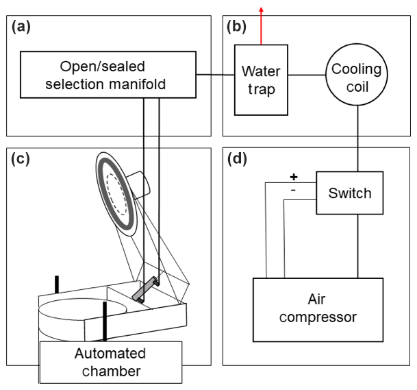
Figure 4Illustration of the chamber pneumatic system that controls opening and closing of chambers. The red arrow denotes the tube to drain the water trap reservoir. Figure panel labels are defined in the main text.
2.4 Principles of chamber gas sampling
Figure 5 outlines the movement of sample gas between chamber and analyzers. Air was pulled through two separate 0.64 cm o.d., 0.43 cm i.d. LDPE plastic tubes. One tube sampled gas adjacent to the chamber inlet tube (Fig. 2), while the second pulled air from the perforated tubing manifold inside the chamber (Fig. 2). The second sampling tube is referred to here as the chamber outlet, as it served to pull ambient air from the chamber inlet tube through the chamber. Both sampling tubes were filtered through 1 µm Teflon (i.e., hydrophobic) filters (Pall Corporation) affixed to LDPE tubing via Swagelok connections immediately outside the chamber to prevent any particulates and liquid water from being pulled through the tubing (Fig. 5a).
Chamber sample selection was achieved by two sets of eight normally closed solenoid valves, one for inlet and one for outlet selection (Clippard, DV-2M-12-L, Fig. 5b). Solenoid valves were controlled by a second Campbell relay controller. Downstream of the chamber selection manifolds, both inlet and outlet gases flowed through additional 1 µm filters. Inlet and outlet flow rates were set independently by two mass flow controllers (Aalborg, GFCS-010201) upstream of two 12V diaphragm gas pumps (KNF Neuberger UNMP830; Fig. 5c). Both flow rates were set to 2 L min−1 by the mass flow controllers, and actual flow rates were recorded on the data logger (which was important for diagnosing potential problems during operation, as discussed later). To mediate selection of the gas sample that flowed to the analyzers, a third sample selection manifold with four normally closed solenoid valves selected among gas sources: chamber inlet, chamber outlet, high concentration standard, or low concentration standard (Fig. 5d). To operate 16 chambers without reducing measurement period or frequency, separate parallel selection manifolds, additional mass flow controllers for chamber inlet/outlet, and diaphragm pumps were added. Two additional solenoid valves on the sample selection manifold allowed selection between each of the two inlet and outlet manifolds. To maintain a constant flow rate through the inlet and outlet sampling tubes when the sample was not being routed to the analyzers, needle valves vented excess flow between the gas pumps and the selection manifold (Fig. 5). The selected sample gas flowed through a common sample gas mass flow controller set to 0.9 L min−1 (Fig. 5e). An internal pump in the N2O analyzer sampled gas at 0.8 L min−1, and this pump also served to pull sample through the CO2 analyzer which had no internal pump. The remaining 0.1 L min−1 was vented through a final needle valve placed upstream of the CO2 analyzer (Fig. 5e).
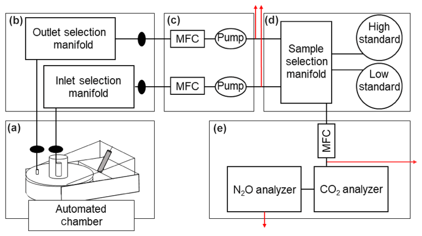
Figure 5Schematic of the sample selection system. Mass flow controllers are abbreviated MFC. Filters are denoted by black ovals. Red arrows indicate where needle valves vent excess flow. Figure panel labels are defined in the main text.
Two instruments in series were used to analyze CO2 and N2O, respectively (Fig. 5e). The CO2 analyzer was placed upstream of the N2O analyzer to avoid artifacts from the high oven temperature and Nafion drying column in the latter. We used a LI-COR 830 (or, subsequently, a LI-COR 850) analyzer to measure CO2 concentrations by infrared absorbance. Downstream, a Teledyne 320U gas filter correlation analyzer measured N2O concentration via infrared absorbance by frequently comparing the sample to a reference gas in a rotating filter (Fassbinder et al., 2013). Instantaneous gas concentrations, as well as the air temperature, inlet flow, outlet flow, and sample flow, were measured every 10 s and recorded on a data logger (Campbell CR3000).
2.5 Measurement principle
Each chamber flux measurement was conducted over the course of a half-hour cycle. When 16 chambers were deployed, a new chamber was closed every 15 min and two chambers were closed simultaneously with the sample gases vented during a 15 min equilibration period prior to a 15 min measurement period. Here we describe the eight-chamber arrangement. To reduce possible conflation between measurement time and plot topographic position, we chose a consistent but staggered plot measurement sequence for each 4 h period (1, 5, 3, 7, 2, 6, 4, 8), where plot one was the lowest topographic position. When 16 chambers were deployed, the plot sequence was maintained so paired chambers at each plot were measured in a single half-hour cycle. At the beginning of each half-hour cycle when a new chamber was going to be measured, a chamber lid was closed by triggering a relay to apply pneumatic pressure to the piston, and the inlet and outlet sampling tubes of the respective chamber began to be sampled at 2 L min−1. Both inlet and outlet tubes were sampled continuously at a constant rate during the half-hour cycle while a downstream selection manifold alternated which gas was routed to the instruments, with residual flow vented to the instrument shed through needle valves (Fig. 5). All pneumatic and sample selection valves were controlled by the data logger. Calibration gases (standards) were measured every 2 h (Fig. 5d). If standards were measured during a given chamber measurement sequence, this was conducted at the beginning of the half-hour period: each standard was measured for 3 min by opening a valve on the gas selection manifold while chamber inlet and outlet flows were vented (Fig. 6a, b). During measurement periods where standards were not measured, the inlet sample was opened first on the selection manifold (Fig. 6c). After 11 min, the inlet was vented while the outlet sample was routed to the instruments until the 16th minute of the half hour (Fig. 6d). The first inlet and outlet gas concentration values from a given chamber measurement cycle (Figs. 6c and 7d respectively) were not used to calculate fluxes, as the chamber headspace concentrations of CO2 and N2O were often not at a steady state during this time. These values, however, were useful for troubleshooting and assessing temporal trends in chamber gas concentrations. Between 16–21 and 21–29 min, the inlet and outlet were respectively measured for a second time (Fig. 6e, f). The minimum 5 min measurement period for inlet and outlet samples was chosen to overcome a lagged response in the N2O analyzer following a switch in sample gas composition, which was as long as 2 min when there were large concentration differences between the inlet and outlet samples; the CO2 analyzer typically stabilized much faster (tens of seconds). The differences between the inlet and outlet gas concentrations averaged over the last 2 min of their second respective measurement periods (Fig. 6e, f) were used to calculate soil gas fluxes (units of ) using Eq. (1). The last 10 s of data from each period were excluded because of transient values during valve switching.
where P is equal to mean atmospheric pressure at our study site (atm), F is the outflow rate (L s−1), ConcOut is the standard-corrected second outlet measurement period gas concentration (µmol mol−1) (Fig. 6f), ConcIn is the standard-corrected second inlet gas concentration (µmol mol−1) (Fig. 6e), R is the ideal gas constant (L atm K−1 mol−1), T is temperature (K), and A is the area covered by the chamber (m2). Following the end of the measurement period (29 min total), the chamber was opened by applying pneumatic pressure to the opposite end of the piston via the open/sealed manifold (Fig. 4a, d) and would remain open prior to the next measurement sequence.
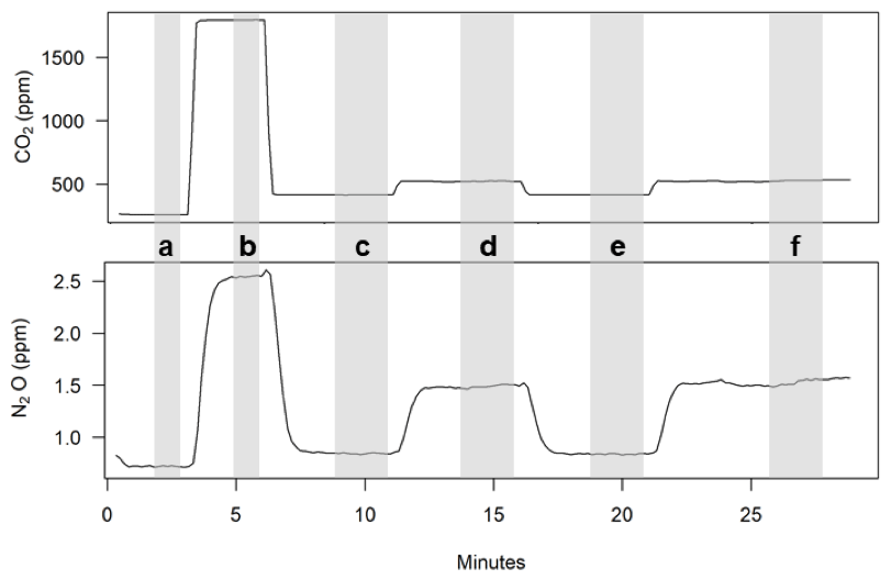
Figure 6Raw instrument output over a representative half-hour chamber measurement period: low standard (a), high standard (b), first inlet measurement (c), first outlet measurement (d), second inlet measurement (e), and second outlet measurement (f). The second set of inlet/outlet measurements was used for flux calculations. Shaded bars indicate periods where output was averaged for subsequent calculations.
Corrected gas concentration values were obtained by applying two-point linear standard corrections updated every 2 h (e.g., Fig. 6a, b). The instrument output during the last minute of each standard measurement, again excluding the last 10 s, was averaged for calibration. Corrected gas concentrations were obtained by regressing measured standard values against known values to obtain a linear slope and intercept used to correct raw values. Working standards were prepared by filling two 50 L gas cylinders with higher and lower concentrations of analytes by mixing CO2- and N2O-free air (zero air) with a concentrated standard gas to achieve values that approximately spanned the range of CO2 and N2O concentrations observed in the field. The mole fractions of each standard gas were verified in our laboratory by analyzing five replicates each on a gas chromatograph (Shimadzu 2014A) with thermal conductivity and electron capture detectors, which were calibrated according to additional NIST-traceable standards using a four-point curve. Gas cylinders filled to 140 MPa lasted approximately 9 months.
All data cleaning, flux calculation, and data analysis were conducted with R statistical software version 3.6.1 (R Core Team, 2019). Cleaning and calibration required R packages lubridate, nlme, and reshape (Grolemund and Wickham, 2011; Pinheiro et al., 2020; Wickham, 2007). The CR3000 data logger code we used to operate the chambers and record data, along with an example dataset and R script for data cleaning and flux calculations, is provided as archived files associated with this publication.
2.6 Power supply: solar panel/batteries
At our field site, six 265 W solar panels (Kyocera) with 16 deep cell marine batteries (Trojan J305E-AC 6V) were able to power the analysis system for much of the year. Figure 7 illustrates the solar charging and battery storage system. Two sets of three solar panels each were wired in series through parallel 15 A circuit breakers within a combiner box. The positive lead flows through a 30 A circuit breaker with a second combiner box before joining the negative at a charge controller (Morningstar TS-MPPT-60, Fig. 7). Indicator lights on the charge controller were used to assess the remaining battery charge, and we occasionally shut the entire system down during prolonged periods of low sunlight to avoid completely discharging the batteries. The charge controller positive output flowed through a 63 A circuit breaker (Fig. 7) to the final positive lead of a battery bank consisting of four sets of four serially wired batteries, each connected in parallel (Fig. 7). The negative output from the charge controller flowed to the negative lead at the opposite end of the battery bank. A 24 V DC output connected to a 60 A breaker (Fig. 7) and a DC/AC converter provided power for the 110 V AC N2O analyzer. A subset of two batteries provided 12 V DC power to the other components (data logger, CO2 analyzer, switches, valves, and additional sensors).
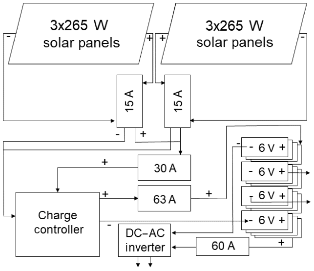
Figure 7Schematic of the solar and power supply system with wiring and circuit breakers. Wires are noted positive (+) and negative (−). Arrows from the DC–AC inverter supply 120 V AC to power the N2O analyzer. Arrows from the battery back supply 12 V DC. Circuit breakers are labeled by their ampere rating. Batteries for the battery bank are labeled by individual battery voltage.
3.1 Troubleshooting
While often no maintenance was required, we typically checked the measurement system every several days to prevent data gaps if a failure occurred. Under ideal conditions (permanent chamber installation, ample sunlight, no flooding), the analysis system may be able to operate over periods of weeks to months without maintenance. However, we found that problems related to chamber submergence, component failure, or unintended faunal interactions occurred on occasion. This section highlights some common issues and practices that we found helpful for addressing them.
3.1.1 Excess moisture
Periodic flooding presented one of the greatest challenges at our field site. Chambers could not sample gas when the water level was above the height of the perforated outlet manifold suspended from the chamber lid (∼7 cm above the soil surface). When water exceeded this height, the filter located at the chamber outlet (Fig. 5a) became saturated with water and stopped flow, preventing damage to the downstream components. If flooding exceeded the height of the inlet (∼30 cm depth), the inlet filter was similarly impacted. Data affected by saturated filters were flagged by noting below-normal inlet/outlet flows during postprocessing and were removed. We replaced saturated filters after the water level receded to return the chamber to operation. Wet filters were dried at 100 ∘C and reused. Excess water also created problems when it condensed downstream of the air compressor. During humid summer conditions the compressor water trap reservoir (Fig. 4c) was emptied at least once every 2 weeks. In subfreezing conditions the trap rarely collected water but was emptied after warmer periods to prevent expansive bursting when temperatures fell below 0 ∘C. Pumps and valves occasionally failed for unknown reasons. In general, we identified problems related to gas flow and sample selection by plotting flow rates over time for each chamber measurement sequence during data postprocessing and replaced any faulty components.
3.1.2 Gnawing animals
Early in our experiment, animals occasionally chewed through the gas tubing between the instrument shed and the chambers. For protection and organization, all four tubes connecting each chamber to the instrument shed (comprising chamber inlet and outlet gas samples, and compressed air for opening and closing the chamber, respectively) were subsequently wrapped in 2.54 cm diameter polyethylene split corrugated wire loom tubing (Drossbach 25D260). The last several cm of each of the four tubes must be able to move independently to allow the piston to move and the chamber lid to open and close. To protect these final portions of tubing which could not be wrapped in protective loom tubing, we replaced the last 30 cm of tubing with semiflexible 0.64 cm diameter copper tubing connected with Swagelok fittings. The copper tubing was molded by hand to enable necessary movement of chamber components and was not impacted by animals. We documented and isolated leaks by capping the chamber end of each tubing line, applying pressure with an air tank to each individual tube, and checking for a drop in regulator pressure. Large leaks were audible and could be easily found and repaired by splicing in replacement tubing using Swagelok union fittings. To test for small leaks, we plumbed the valves to a tank of industrial-grade helium and used a helium-specific leak detector (Restek 28500). After protecting against animal damage, leaks were infrequent.
3.1.3 Power limitation
We experienced occasional power outages during extended periods of cloudy weather and during winter. By periodically turning the analysis system off for several days to allow the batteries to reach full charge, we could collect 2–3 d of measurements even in cold/cloudy conditions. During periods of chamber closure (3 out of every 24 h during typical operation), rainfall was excluded from the chamber enclosure, which could potentially alter soil moisture. Elsewhere, a rain gauge has been used to signal automated chambers to remain open during rainfall events (Butterbach-Bahl and Dannenmann, 2011). Here, we elected to maintain a consistent measurement schedule irrespective of rainfall, due to the logistical challenges posed by prolonged rainfall events (when no measurements would be collected). A rainfall rate threshold required to open the automated chambers could be useful in future studies to limit the frequency and duration of data gaps. Future measurements will also quantify the potential magnitude of any soil moisture effect associated with our automated chamber system. To reduce the duration that the chambers were closed when the system was off for power conservation or maintenance, we either left the compressor on and the chambers in the open position or propped the chambers open. The Teledyne N2O analyzer has an internal component (heated to near 70 ∘C) which consumed additional power during cold weather. We found that enclosing the N2O analyzer in a plywood box with 2.54 cm polystyrene foam insulation on four sides (leaving one side and the back open for ventilation) reduced power use. We also adjusted the angle of the solar array at least twice a year to increase efficiency. Collectively, these energy-efficient measures allowed the instrument to operate for longer periods when solar energy was limiting. Occasionally, however, the DC/AC converter would shut down during the night due to power limitation and would turn on again when sunlight was available. Data from the N2O analyzer were consistently biased during an 8 h period as the instrument warmed up. We flagged and discarded these data during postprocessing by plotting analyzer output over time and removing peaks following periods where no output was recorded.
3.2 Measurement assumptions
A key principle of steady-state chamber operation is that the gas concentration inside the chamber headspace is approximately at equilibrium (gas flux from the soil is balanced with gas removed via the chamber outlet) when the flux measurement is made. The time to achieve steady-state conditions is a balance between the soil flux rate and the flow of gas through the chamber. Here, to enable the use of smaller pumps and conserve power we employed lower flow rates (2 L min−1) than often employed previously in dynamic chambers (e.g., 4 L min−1; Bowling et al., 2015). Initial tests revealed that use of larger pumps needed to achieve 4 L min−1 flow rates over >100 m tubing runs was not sustainable from the perspective of power supply. To validate the steady-state assumption at 2 L min−1, we analyzed the slope of a linear regression between concentration of CO2 and N2O and time over the final outlet measurement period (Fig. 6f, approximately 27–29 min) using data from three separate periods chosen to cover a broad range of fluxes and spanning 2 weeks in total. We found an average increase of 0.18±10.51 ppm CO2 min−1 (mean and SD) and 0.57±8.40 ppb N2O min−1, respectively, indicating that both gases were approximately at a steady state at the end of the measurement period (relative to mean chamber outlet values of 684 ppm and 494 ppb for CO2 and N2O, respectively). We repeated this analysis for the final inlet measurement period (Fig. 6e, approximately 19–21 min) and found a change of less than 1 ppm or ppb min−1 CO2 and N2O relative to mean chamber inlet concentrations of 539 ppm and 331 ppb, respectively.
To assess temperature sensitivity of both gas analyzers under field conditions we examined the slope and intercept of standard curves measured during a 20 d period when air temperature ranged from −4 to 21 ∘C and during which the instruments ran continuously. There was no significant directional trend in air temperature over this period to avoid conflating temperature-related drift and drift of the instrument over time unrelated to temperature. All four metrics examined (slope and intercept of CO2 and N2O calibration curves) displayed correlations with temperature. However, the impact of temperature on the slope of the CO2 and N2O calibrations was less than 10−3 ppm ∘C−1 for both values. These values correspond to <1 % difference in instrument output between the highest and lowest observed temperature values at CO2 and N2O concentrations of 400 and 0.3 ppm, respectively. The intercept values showed greater sensitivity (0.02 and 0.003 ppm ∘C−1 for CO2 and N2O, respectively). These values correspond to a ∼0.5 ppm difference in CO2 and ∼0.08 ppm difference in N2O at the high and low temperature range observed. Taken together, we found that the N2O instrument had a −0.006 ppm ∘C−1 sensitivity, in close agreement to the −0.009 ppm ∘C−1 found by Fassbinder et al. (2013) for a similar instrument from the same manufacturer. As detailed above, standards were measured every 2 h to account for instrument sensitivity to environmental conditions. Additionally, because gas flux was calculated as the difference between and inlet and outlet concentration the intercept values canceled mathematically, thereby removing any additional bias due to temperature-related intercept drift between standard measurements. Therefore, temperature variation between measurements had negligible impact on the final flux calculation.
Optical trace gas measurements may be affected by a number of interacting factors including temperature, pressure, and water vapor pressure (McDermitt et al., 1993). Water vapor can be removed through chemical traps. However, the high gas flow in our system (2 L min−1) made reagent replacement in chemical traps impractical, and preliminary work showed that membrane-based driers did not always completely remove water vapor in our operating environment, where relative humidity often reached 100 %. The N2O analyzer we utilized removed moisture through a multitube Nafion dryer (Model NMP850KNDCB, KNF Neuberger Inc.). Water vapor was not removed prior to measuring CO2 concentration. As we calculated the soil CO2 flux as proportional to the concentration difference between the inlet and outlet gases, we were primarily concerned with a change in water vapor between the inlet and outlet measurement (Fig. 6e, f). In 2019, measurements were made with a LI-COR 850 that included a water vapor correction and measurement, which we used to constrain the potential impact of water vapor on our previous CO2 measurements. McDermitt et al. (1993) found that the required water vapor correction using a similar analysis was <10 ppm CO2 at water vapor pressure of 25.3 mmol mol−1 and CO2 concentration up to 1000 ppm. Water vapor pressure in the gases we measured spanned 1.0–53.6 mmol mol−1, with an average difference between the inlet and outlet gas of 1.8 mmol mol−1 and a maximum of 36.4 mmol mol−1. These small observed changes in water vapor between the inlet and outlet measurements indicate a minor impact on measured CO2 fluxes: if the water vapor difference between the inlet and outlet caused a <10 ppm bias in the measured CO2 concentration (as expected in >99.9 % of our observations), this would impact the average measured CO2 flux (3.47 ) by <5.2 % (0.18 ), which is within the typical range of measurement uncertainty for reproducing a known flux value under controlled conditions (Pumpanen et al., 2004). The correction under a more moderate water vapor difference between the inlet and outlet (<12.6 mmol mol−1) that spans >97 % of observed differences is approximately half the impact of this extreme example (0.09 ). Unrelated to its impacts on instrument performance, water vapor can also impact flux measurements by dilution (Harazono et al., 2015). Given an average water vapor difference between the inlet and outlet of 1.8 mmol mol−1 and maximum of 36.4 mmol mol−1, impacts of dilution on measured fluxes would also be small: typically <0.18 % and as much as 3.6 %.
To constrain the potential impacts of water vapor on measured N2O concentrations, we conducted a laboratory experiment comparing the N2O instrument output between a high and low moisture measurement on a three-point standard curve. Water vapor was measured with a LI-COR 850 installed in-line and upstream of the N2O sensor. To quantify the impact of water vapor on instrument output, we compared the standard curve created from dry standards to a curve created after bubbling the gas through a jar of deionized water. The bubbling technique added a mean of 25.4 mmol mol−1 of water vapor, spanning >99.9 % of observations of the difference between water vapor at the inlet and outlet in the field. Standard gases ranged up to 9.96 ppm N2O, greater than all differences between the inlet and outlet observed in the field. No difference was noted in N2O instrument output due to the presence of water vapor, which suggested the drying column was effective at removing water vapor or that the gas filter correlation method corrected for any impacts of residual vapor.
3.3 Temporal dynamics
Manual trace gas sampling by field crews is generally accomplished during normal daytime work hours. In contrast, automated measurements can be scheduled throughout the 24 h diel period. Figure 8 displays boxplots of N2O emission from days when chambers were measured at each 4 h interval during 2017 and 2019 (the years of Zea mays cultivation). Though infrequent, we observed occasional instantaneous negative N2O flux values, as observed in other ecosystems (Schlesinger, 2013; Wu et al., 2013). Figure 9 shows the N2O and CO2 emissions from two typical 1-week periods from September 2017 and August 2018. A diel trend is visible for most chambers in August and some chambers and time periods in September. In general agreement with previously published automated chamber N2O studies from agricultural soils, we found the lowest rates of emission during early morning (04:00–08:00 LT) and highest emissions during early afternoon (12:00–16:00 LT) (Akiyama et al., 2000; Alves et al., 2012; Bai et al., 2019; Flessa et al., 2002; Savage et al., 2014). Early afternoon measurements were on average 28 % greater than the daily average from each chamber (4.04 vs. 3.15 nmol m−2 s−1), but this difference varied from −13.9 to 110 nmol m−2 s−1 among all chambers/days that were compared. The relative difference between average and peak daily emissions was in reasonable agreement with previous data from agricultural fields in the United Kingdom, Australia, and the United States (approximately 31, 47, and 33 % respectively; Alves et al., 2012; Bai et al., 2019; Savage et al., 2014). Although CO2 fluxes were highest and lowest during the same time periods as N2O, early afternoon CO2 fluxes were 22 % greater than the daily mean, on average (4.38 and 3.60 ), and this difference varied between −7.72 and 21.1 among all chambers/days that were compared.
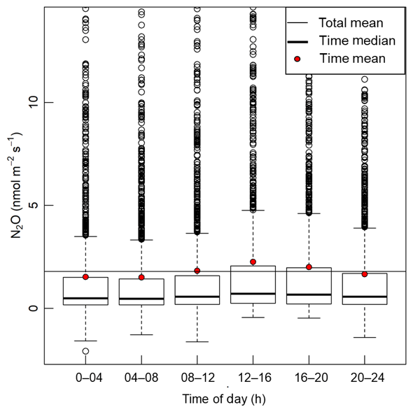
Figure 8Boxplot of N2O fluxes during each 4 h interval. Positive outliers >14 nmol m−2 s−1 that comprised 1.9 % of the total dataset are not shown for clarity.
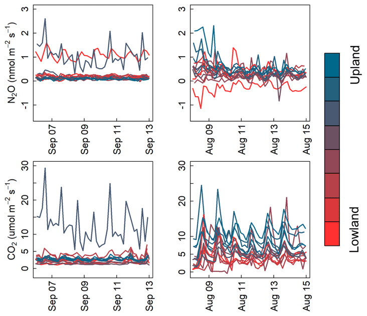
Figure 9N2O and CO2 flux time series shaded by plot topographic location over two 1-week periods in September 2017 and August 2018.
N2O emissions pulses have often been observed following rain events (Savage et al., 2014; Sehy et al., 2003). To assess the length of the delay between rainfall and peak emissions, we analyzed the number of hours between heavy rainfall (defined as >2 cm total over 24 h) and subsequent peak N2O emission rate averaged over all chambers. A rain gauge located on-site recorded precipitation data that were obtained through the Iowa Flood Center (2017). There were 45 d with total rainfall >2 cm. To avoid conflating more than one rain event, we chose isolated events without rainfall >4 mm d−1 in the preceding or the following 2 d. Of the 15 isolated rain events observed, 4 were analyzed that did not span data gaps (Fig. 10). The rain-to-peak-emission delay varied from 12 to 26 h among precipitation events which varied from 2.4 to 4.4 cm.

Figure 10N2O flux time series shaded by plot topographic location over four 1-week periods in May 2017, August 2017, September 2017, and May 2019. The dashed black lines denote rain events analyzed for peak delay, and gray lines indicate rain events that did not fit our selection criteria and were >2 mm d−1.
Our results indicate that steady-state flux conditions were achieved under reasonable periods of chamber closure (29 min), equivalent to the common 30 min averaging interval for eddy covariance measurements (Loescher et al., 2006) and flow rates (2 L min−1) that could be attained using low-power 12 V pumps. The results were minimally impacted by measurement error due to water vapor and were robust to changes in air temperature. We applied our high-frequency data to address two questions, how strong does diel variation impact trace gas emissions and how long is the delay between precipitation and the frequently observed pulse in N2O. Our observations showed that the average daily emissions were most closely approximated by measurements made between 08:00 and 12:00 LT. Although CO2 emissions were best approximated during the same time interval, the difference between peak emissions and the daily average was less pronounced and displayed less variability than observed for N2O. We found the delay between rainfall and peak N2O emissions varied between 12 and 26 h – intervals that would be difficult to capture using manual sampling methods. Both findings of temporal variability support the need for high-frequency measurements to calculate annual soil trace gas emissions budgets. This measurement system could also be adapted to study other gases provided that the gas analyzers chosen are able to tolerate field conditions. In particular, the steady-state chamber design used here provides a powerful tool for future studies to couple gas flux with isotopic measurements that may uncover the source and processes underlying the observed flux.
Agricultural management required us to remove the chambers and associated equipment several times of year. Without these constraints, experiments utilizing this method could examine processes that take place on even greater spatial scales than those utilized here (tubing runs >100 m) and with a greater number of chambers. Despite these challenges, we were able to construct and maintain eight (with one spare) high-frequency automated chambers for subdaily N2O and CO2 flux measurements in a temperate agricultural field, with a total materials cost (∼ USD 40 000, including parts for nine chambers, gas analyzers, control system, and power supply) that is a fraction of the cost of many laser-based N2O analyzers alone. We estimate that the chambers and control system took us 130–260 h to construct and troubleshoot (with concomitant labor/salary costs) and did not require specialized tools beyond those available in a typical workshop.
Raw data, data logger code, and data processing scripts are available from the Iowa State University DataShare repository at https://doi.org/10.25380/iastate.12550790 (Lawrence and Hall, 2020).
The supplement related to this article is available online at: https://doi.org/10.5194/amt-13-4065-2020-supplement.
NCL and SJH jointly designed and carried out research and prepared the manuscript.
The authors declare that they have no conflict of interest.
We thank Carlos Tenesaca, Anthony Mirabito, Lucio Reyes, and Lindsay Mack for field assistance, as well as Dave Bowling for critical advice regarding chamber construction.
This research has been supported by the USDA (award no. 2018-67019-27886), the Leopold Center for Sustainable Agriculture (award no. E2017-02), and the Iowa Nutrient Research Center (award no. 109-47-03-39-3650).
This paper was edited by Christian Brümmer and reviewed by two anonymous referees.
Akiyama, H., Tsuruta, H., and Watanabe, T.: N2O and NO emissions from soils after the application of different chemical fertilizers, Chemosphere, 2, 313–320, https://doi.org/10.1016/S1465-9972(00)00010-6, 2000.
Alves, B. J. R., Smith, K. A., Flores, R. A., Cardoso, A. S., Oliveira, W. R. D., Jantalia, C. P., Urquiaga, S., and Boddey, R. M.: Selection of the most suitable sampling time for static chambers for the estimation of daily mean N2O flux from soils, Soil Biol. Biochem., 46, 129–135, https://doi.org/10.1016/j.soilbio.2011.11.022, 2012.
Ambus, P. and Robertson, G. P.: Automated near-continuous measurement of carbon dioxide and nitrous oxide fluxes from soil, Soil Sci. Soc. Am. J., 62, 394–400, https://doi.org/10.2136/sssaj1998.03615995006200020015x, 1998.
Bai, M., Suter, H., Lam, S. K., Flesch, T. K., and Chen, D.: Comparison of slant open-path flux gradient and static closed chamber techniques to measure soil N2O emissions, Atmos. Meas. Tech., 12, 1095–1102, https://doi.org/10.5194/amt-12-1095-2019, 2019.
Barton, L., Wolf, B., Rowlings, D., Scheer, C., Kiese, R., Grace, P., Stefanova, K., and Butterbach-Bahl, K.: Sampling frequency affects estimates of annual nitrous oxide fluxes, Scientific Reports, 5, 15912, https://doi.org/10.1038/srep15912, 2015.
Bowling, D. R., Egan, J. E., Hall, S. J., and Risk, D. A.: Environmental forcing does not induce diel or synoptic variation in the carbon isotope content of forest soil respiration, Biogeosciences, 12, 5143–5160, https://doi.org/10.5194/bg-12-5143-2015, 2015.
Breuer, L., Papen, H., and Butterbach-Bahl, K.: N2O emission from tropical forest soils of Australia, Res., 105, 26353–26367, https://doi.org/10.1029/2000JD900424, 2000.
Butterbach-Bahl, K. and Dannenmann, M.: Denitrification and associated soil N2O emissions due to agricultural activities in a changing climate, Cur. Opin. Env. Sust., 3, 389–395, https://doi.org/10.1016/j.cosust.2011.08.004, 2011.
Butterbach-Bahl, K., Gasche, R., Breuer, L., and Papen, H.: Fluxes of NO and N2O from temperate forest soils: impact of forest type, N deposition and of liming on the NO and N2O emissions, Nutr. Cycl. Agroecosys., 48, 79–90, https://doi.org/10.1023/A:1009785521107, 1997.
Courtois, E. A., Stahl, C., Burban, B., Van den Berge, J., Berveiller, D., Bréchet, L., Soong, J. L., Arriga, N., Peñuelas, J., and Janssens, I. A.: Automatic high-frequency measurements of full soil greenhouse gas fluxes in a tropical forest, Biogeosciences, 16, 785–796, https://doi.org/10.5194/bg-16-785-2019, 2019.
Davidson, E. A., Savage, K., Verchot, L. V., and Navarro, R.: Minimizing artifacts and biases in chamber-based measurements of soil respiration, Ag. Forest Meteorol., 113, 21–37, https://doi.org/10.1016/S0168-1923(02)00100-4, 2002.
Fang, C. and Moncrieff, J. B.: An open-top chamber for measuring soil respiration and the influence of pressure difference on CO2 efflux measurement, Funct. Ecol., 12, 319–325, https://doi.org/10.1046/j.1365-2435.1998.00189.x, 1998.
Fassbinder, J. J., Schultz, N. M., Baker, J. M., and Griffis, T. J.: Automated, low-power chamber system for measuring nitrous oxide emissions, J. Environ. Qual., 42, 606–614, https://doi.org/10.2134/jeq2012.0283, 2013.
Flessa, H., Ruser, R., Schilling, R., Loftfield, N., Munch, J. C., Kaiser, E. A., and Beese, F.: N2O and CH4 fluxes in potato fields: automated measurement, management effects and temporal variation, Geoderma, 105, 307–325, https://doi.org/10.1016/S0016-7061(01)00110-0, 2002.
Groffman, P. M., Altabet, M. A., Böhlke, J. K., Butterbach-Bahl, K., David, M. B., Firestone, M. K., Giblin, A. E., Kana, T. M., Nielsen, L. P., and Voytek, M. A.: Methods for measuring denitrification: diverse approaches to a difficult problem, Ecol. Appl., 16, 2091–2122, https://doi.org/10.1890/1051-0761(2006)016[2091:MFMDDA]2.0.CO;2, 2006.
Groffman, P. M., Butterbach-Bahl, K., Fulweiler, R. W., Gold, A. J., Morse, J. L., Stander, E. K., Tague, C., Tonitto, C., and Vidon, P.: Challenges to incorporating spatially and temporally explicit phenomena (hotspots and hot moments) in denitrification models, Biogeochemistry, 93, 49–77, https://doi.org/10.1007/s10533-008-9277-5, 2009.
Grolemund, G. and Wickham, H.: Dates and times made easy with lubridate, J. Stat. Softw., 40, 1–25, https://doi.org/10.18637/jss.v040.i03, 2011.
Harazono, Y., Iwata, H., Sakabe, A., Ueyama, M., Takahashi, K., Nagano, H., Nakai, T., and Kosugi, Y.: Effects of water vapor dilution on trace gas flux, and practical correction methods, J. Agric. Meteorol., 71, 65–76, https://doi.org/10.2480/agrmet.D-14-00003, 2015.
Hutchinson, G. L. and Mosier, A. R.: Improved soil cover method for field measurement of nitrous oxide fluxes, Soil Sci. Soc. Am. J., 45, 311–316, https://doi.org/10.2136/sssaj1981.03615995004500020017x, 1981.
Iowa Flood Center: Iowa Flood Information System, available at: http://ifis.iowafloodcenter.org (last access: 21 November 2019), 2017.
Lawrence, N. and Hall, S.: Files accompanying “Capturing temporal heterogeneity in soil nitrous oxide fluxes with a robust and low-cost automated chamber apparatus”, Iowa State University, https://doi.org/10.25380/iastate.12550790, 2020.
Loescher, H. W., Law, B. E., Mahrt, L., Hollinger, D. Y., Campbell, J., and Wofsy, S. C.: Uncertainties in, and interpretation of, carbon flux estimates using the eddy covariance technique, J. Geophys. Res., 111, D21S90, https://doi.org/10.1029/2005JD006932, 2006.
Logsdon, S. D. and James, D. E.: Closed depression topography Harps soil, revisited, Soil Horizons, 55, 1–7, https://doi.org/10.2136/sh13-11-0025, 2014.
McDermitt, D. K., Welles, J. M., and Eckles, R. D.: Effects of temperature, pressure and water vapor on gas phase infrared absorption by CO2, available at: https://www.licor.com/documents/sul40zcvtnr8t71arbua (last access: 21 November 2019), 1993.
Merbold, L., Wohlfahrt, G., Butterbach-Bahl, K., Pilegaard, K., DelSontro, T., Stoy, P. and Zona, D.: Preface: Towards a full greenhouse gas balance of the biosphere, Biogeosciences, 12, 453–456, https://doi.org/10.5194/bg-12-453-2015, 2015.
Minasny, B., Malone, B. P., McBratney, A. B., Angers, D. A., Arrouays, D., Chambers, A., Chaplot, V., Chen, Z.-S., Cheng, K., Das, B. S., Field, D. J., Gimona, A., Hedley, C. B., Hong, S. Y., Mandal, B., Marchant, B. P., Martin, M., McConkey, B. G., Mulder, V. L., O'Rourke, S., Richer-de-Forges, A. C., Odeh, I., Padarian, J., Paustian, K., Pan, G., Poggio, L., Savin, I., Stolbovoy, V., Stockmann, U., Sulaeman, Y., Tsui, C.-C., Vågen, T.-G., van Wesemael, B., and Winowiecki, L.: Soil carbon 4 per mille, Geoderma, 292, 59–86, https://doi.org/10.1016/j.geoderma.2017.01.002, 2017.
Moyes, A. B., Schauer, A. J., Siegwolf, R. T. W., and Bowling, D. R.: An injection method for measuring the carbon isotope content of soil carbon dioxide and soil respiration with a tunable diode laser absorption spectrometer, Rapid Commun. Mass Sp., 24, 894–900, https://doi.org/10.1002/rcm.4466, 2010a.
Moyes, A. B., Gaines, S. J., Siegwolf, R. T. W., and Bowling, D. R.: Diffusive fractionation complicates isotopic partitioning of autotrophic and heterotrophic sources of soil respiration, Plant Cell Environ., 33, 1804–1819, https://doi.org/10.1111/j.1365-3040.2010.02185.x, 2010b.
Nickerson, N. and Risk, D.: Physical controls on the isotopic composition of soil-respired CO2, J. Geophys. Res., 114, G01013, https://doi.org/10.1029/2008JG000766, 2009.
Norman, J. M., Kucharik, C. J., Gower, S. T., Baldocchi, D. D., Crill, P. M., Rayment, M., Savage, K., and Striegl, R. G.: A comparison of six methods for measuring soil-surface carbon dioxide fluxes, J. Geophys. Res., 102, 28771–28777, https://doi.org/10.1029/97JD01440, 1997.
Papen, H. and Butterbach-Bahl, K.: A 3-year continuous record of nitrogen trace gas fluxes from untreated and limed soil of a N-saturated spruce and beech forest ecosystem in Germany: 1. N2O emissions, J. Geophys. Res., 104, 18487–18503, https://doi.org/10.1029/1999JD900293, 1999.
Parkin, T. B.: Effect of sampling frequency on estimates of cumulative nitrous oxide emissions, J. Environ. Qual., 37, 1390–1395, https://doi.org/10.2134/jeq2007.0333, 2008.
Paustian, K., Lehmann, J., Ogle, S., Reay, D., Robertson, G. P., and Smith, P.: Climate-smart soils, Nature, 532, 49–57, https://doi.org/10.1038/nature17174, 2016.
Pihlatie, M., Rinne, J., Ambus, P., Pilegaard, K., Dorsey, J. R., Rannik, Ü., Markkanen, T., Launiainen, S., and Vesala, T.: Nitrous oxide emissions from a beech forest floor measured by eddy covariance and soil enclosure techniques, Biogeosciences, 2, 377–387, https://doi.org/10.5194/bg-2-377-2005, 2005.
Pinheiro, J., Bates, D., DebRoy, S., Sarkar, D., and R Core Team: nlme: linear and nonlinear mixed effects models, R package version 3.1-140, available at: https://cran.r-project.org/web/packages/nlme/index.html, last access: 1 June 2020.
Pumpanen, J., Kolari, P., Ilvesniemi, H., Minkkinen, K., Vesala, T., Niinistö, S., Lohila, A., Larmola, T., Morero, M., Pihlatie, M., Janssens, I., Yuste, J. C., Grünzweig, J. M., Reth, S., Subke, J.-A., Savage, K., Kutsch, W., Østreng, G., Ziegler, W., Anthoni, P., Lindroth, A., and Hari, P.: Comparison of different chamber techniques for measuring soil CO2 efflux, Agr. Forest Meteorol., 123, 159–176, https://doi.org/10.1016/j.agrformet.2003.12.001, 2004.
Rayment, M. B. and Jarvis, P. G.: An improved open chamber system for measuring soil CO2 effluxes in the field, J. Geophys. Res., 102, 28779–28784, https://doi.org/10.1029/97JD01103, 1997.
R Core Team: R: A Language and Environment for Statistical Computing, R Foundation for Statistical Computing, Vienna, Austria, available at: https://www.R-project.org/ (last access: 1 June 2020), 2019.
Riggs, A. C., Stannard, D. I., Maestas, F. B., Karlinger, M. R., and Striegl, R. G.: Soil CO2 flux in the Amargosa Desert, Nevada, during El Nino 1998 and La Nina 1999, US Geol. Surv. Sci. Investig. Rep., 2009–5061, 25 pp., available at: https://pubs.usgs.gov/sir/2009/5061/ (last access: 1 June 2020), 2009.
Rosenstock, T. S., Diaz-Pines, E., Zuazo, P., Jordan, G., Predotova, M., Mutuo, P., Abwanda, S., Thiong'o, M., Buerkert, A., Rufino, M. C., Kiese, R., Neufeldt, H., and Butterbach-Bahl, K.: Accuracy and precision of photoacoustic spectroscopy not guaranteed, Glob. Change Biol., 19, 3565–3567, https://doi.org/10.1111/gcb.12332, 2013.
Savage, K., Phillips, R., and Davidson, E.: High temporal frequency measurements of greenhouse gas emissions from soils, Biogeosciences, 11, 2709–2720, https://doi.org/10.5194/bg-11-2709-2014, 2014.
Schlesinger, W. H.: An estimate of the global sink for nitrous oxide in soils, Glob. Change Biol., 19, 2929–2931, https://doi.org/10.1111/gcb.12239, 2013.
Sehy, U., Ruser, R., and Munch, J. C.: Nitrous oxide fluxes from maize fields: relationship to yield, site-specific fertilization, and soil conditions, Agr. Ecosyst. Environ., 99, 97–111, https://doi.org/10.1016/S0167-8809(03)00139-7, 2003.
Wickham, H.: Reshaping data with the reshape package, J. Stat. Softw., 21, 1–20, https://doi.org/10.18637/jss.v021.i12, 2007.
Wu, D., Dong, W., Oenema, O., Wang, Y., Trebs, I., and Hu, C.: N2O consumption by low-nitrogen soil and its regulation by water and oxygen, Soil Biol. Biochem., 60, 165–172, https://doi.org/10.1016/j.soilbio.2013.01.028, 2013.
Xu, L., Furtaw, M. D., Madsen, R. A., Garcia, R. L., Anderson, D. J., and McDermitt, D. K.: On maintaining pressure equilibrium between a soil CO2 flux chamber and the ambient air, J. Geophys. Res., 111, D08S10, https://doi.org/10.1029/2005JD006435, 2006.