CLIMCAPS observing capability for temperature, moisture, and trace gases from AIRS/AMSU and CrIS/ATMS

The Community Long-term Infrared Microwave Combined Atmospheric Product System (CLIMCAPS) retrieves vertical profiles of temperature, water vapor, greenhouse and pollutant gases, and cloud properties from measurements made by infrared and microwave instruments on polar-orbiting satellites. These are AIRS/AMSU on Aqua and CrIS/ATMS on Suomi NPP and NOAA20; together they span nearly 2 decades of daily observations (2002 to present) that can help characterize diurnal and seasonal atmospheric processes from different time periods or regions across the globe. While the measurements are consistent, their information content varies due to uncertainty stemming from (i) the observing system (e.g., instrument type and noise, choice of inversion method, algorithmic implementation, and assumptions) and (ii) localized conditions (e.g., presence of clouds, rate of temperature change with pressure, amount of water vapor, and surface type). CLIMCAPS quantifies, propagates, and reports all known sources of uncertainty as thoroughly as possible so that its retrieval products have value in climate science and applications. In this paper we characterize the CLIMCAPS version 2.0 system and diagnose its observing capability (ability to retrieve information accurately and consistently over time and space) for seven atmospheric variables – temperature, H₂O, CO, O₃, CO₂, HNO₃, and CH₄ – from two satellite platforms, Aqua and NOAA20. We illustrate how CLIMCAPS observing capability varies spatially, from scene to scene, and latitudinally across the globe. We conclude with a discussion of how CLIMCAPS uncertainty metrics can be used in diagnosing its retrievals to promote understanding of the observing system and the atmosphere it measures.

1 Introduction

Instruments onboard satellites observe the global Earth atmosphere with unprecedented regularity in space and time. For any given scene on Earth today there are multiple observations from a range of different instruments measuring any number of atmospheric variables. While the record of hyperspectral infrared measurements spans nearly 2 decades, differences in technology and instrumentation pose a significant challenge to data continuity (Smith et al., 2013). Two space-based systems may observe the same atmospheric variable but at different view angles, different times of day, and different spatial or spectral resolutions, measuring different aspects of the Earth's atmosphere. The challenge in intercomparing different sources of remote observations is well documented (Stubenrauch et al., 1999; Rodgers and Connor, 2003; Wylie et al., 2005; von Clarmann and Grabowski, 2007; Smith et al., 2013, 2015; Hearty et al., 2014; Gaudel et al., 2018). Straightforward side-by-side comparisons of disparate data sets can fail to yield meaningful insights because their differences cannot be explained by natural variability or instrument capability alone. Uncertainty masks the measured signal. Only with rigorous quantification and deliberate propagation of uncertainty through all data processing steps can a degree of transparency in space-based observations be achieved so that the measured signal can be distinguished, uncertainty can be characterized, and data set differences can be understood (Pougatchev et al., 1996; Ceccherini et al., 2003; Pougatchev, 2008; Ceccherini and Ridolfi, 2010; Hulley et al., 2012; Xiong et al., 2013; Merchant et al., 2017, 2019).

Pougatchev (2008) classified uncertainty in remote observations into two primary sources, namely (i) “state noncoincidence” or scene-dependent effects, such as spatial heterogeneity and temporal variation, and (ii) “characteristic differences” or observing system effects such as spectral resolution, footprint size, and retrieval algorithm design. Uncertainty, irrespective of its source, can be random (unreproducible) or systematic (reproducible). Random uncertainty can average out when data are aggregated, but systematic uncertainty propagates through analysis steps and obscures the measured signal in final results (Smith et al., 2015). It is therefore imperative to characterize systematic uncertainty as rigorously as possible.

In this paper we focus on satellite sounding systems that retrieve atmospheric variables as vertical profiles from top-of-atmosphere radiance measurements, more specifically on the Community Long-term Infrared Microwave Combined Atmospheric Product System (CLIMCAPS; Smith and Barnet, 2019). CLIMCAPS is the National Aeronautics and Space Administration (NASA) system for sounder instruments on the polar-orbiting satellites Aqua (2002–present), Suomi NPP (2012–present), and NOAA20 (2017–present) that is the first of the Joint Polar Satellite System (JPSS) series of four satellites scheduled to maintain operational orbit through 2040. CLIMCAPS implements Bayesian optimal estimation (OE) (Rodgers, 2000) as an inversion technique and employs explicit background error quantification with uncertainty propagation. Other sounding systems offer variations of the OE approach in practice, depending on their respective data product requirements (Susskind et al., 2003, 2014; Fu et al., 2016; DeSouza-Machado et al., 2018; Irion et al., 2018). We designed CLIMCAPS to achieve and maintain consistent observing capability across different satellite platforms so that we can generate a long-term, continuous record of satellite soundings for a nearly 2-decade period of hyperspectral infrared (IR) observations from space.

Smith and Barnet (2019) described how CLIMCAPS quantifies and propagates scene-dependent uncertainty using error covariance matrices (ECMs) in a sequential retrieval approach that starts with retrieving clouds, followed by temperature, water vapor, and the trace gas species O₃, CO, CH₄, CO₂, N₂O, SO₂, and HNO₃. Averaging kernel matrices (AKMs) characterize the degree to which each of the retrieved variables depends on information contributed by the measurements about the true state of that variable. Averaging kernels have value in data intercomparison studies (Rodgers and Connor, 2003; Maddy and Barnet, 2008; Maddy et al., 2009; Gaudel et al., 2018; Iturbide-Sanchez et al., 2017) and form a critical component of data assimilation models (Levelt et al., 1998; Clerbaux et al., 2001; Yudin, 2004; Segers et al., 2005; Pierce et al., 2009; Liu et al., 2012).

We present CLIMCAPS version 2.0 AKMs for a range of different retrieval variables, different scenes across time and space, and multiple satellite platforms and instrument types with the goal of characterizing CLIMCAPS observing capability and promoting a better understanding of its retrieved soundings and their value in applications.

Terminology and notation

We define an observing system, such as CLIMCAPS, as the space-based instrument along with its inversion algorithm. Observing system characteristics that affect product quality include spectral resolution, spatial footprint (“pixel” or “field of view”) size, shape, arrangement, instrument noise, view angles across satellite swath, which for CrIS is 2200 km (±50^∘), and effects due to the regularization and stabilization of its retrieval algorithm. With observing system capability, we mean the potential a space-based system has for measuring the atmospheric state at a specific scene given the instrument type, retrieval system design, and prevailing conditions. Observing capability is akin to the signal-to-noise ratio (SNR) and should ideally be high enough to add independent, new information to background knowledge about the atmospheric state at any given point in time and space. CLIMCAPS employs Bayesian inversion as a retrieval scheme and generates AKMs to quantify the sensitivity of retrieved variables to the true state of those variables (Rodgers, 2000) as a metric of uncertainty. CLIMCAPS product files available through the NASA Earth Observing System Data and Information System (EOSDIS; Ramapriyan et al., 2010) contain AKMs for seven retrieval variables – temperature (T), water vapor (H₂O), ozone (O₃), carbon monoxide (CO), methane (CH₄), carbon dioxide (CO₂), and nitric acid (HNO₃) – at every scene. We define a CLIMCAPS retrieval scene (or “field of regard”) as the spatial and spectral aggregate of radiance measurements that results from performing cloud clearing (Chahine, 1982; Susskind et al., 1998; Smith and Barnet, 2019). Cloud clearing removes the radiative effect of clouds from IR measurements by aggregating cloud-sensitive channels from nine neighboring CrIS (or AIRS) instrument footprints. Cloud clearing requires no prior knowledge of scene-specific cloud properties nor does it depend on radiative transfer calculations through clouds. Instead, cloud clearing is a robust linear method that uses the 3×3 spatial cluster of instrument footprints as spectrally independent information about scene cloudiness and, together with knowledge of the cloud-free state retrieved from coincident microwave measurements (ATMS or AMSU), derives a set of cloud-cleared spectral channels for use in subsequent retrievals. In the case in which no clouds are detected, the relevant channels are simply averaged across the 3×3 array (nine footprints in total) with the assumption that it is a uniformly clear scene. While CLIMCAPS aggregates spectral radiance before retrieval (known as an “average-then-retrieve” approach), the retrieved soundings are still considered instantaneous observations because CLIMCAPS limits its radiance aggregation to small spatial clusters (an aggregate scene of 3×3 CrIS footprints has ∼50 km diameter at nadir and ∼150 km at the edge of a scan) and performs no temporal averaging ahead of inversion. We use the term measurement to refer to the measured spectrum (i.e., top-of-atmosphere radiance either for a single footprint or cloud-cleared scene) and distinguish it from retrieval, which is the inverse measurement or retrieved pressure-dependent atmospheric variable at every scene (e.g., water vapor). We maintain consistency with the mathematical notations adopted by Rodgers (2000) for the sake of simplicity and relevance to other OE systems (Bowman et al., 2006; Ceccherini et al., 2009; Ceccherini and Ridolfi, 2010; Fu et al., 2016; DeSouza-Machado et al., 2018; Irion et al., 2018); a measured spectrum is represented by the vector y with m spectral channels, and the retrieved parameter is represented by vector x with n vertical pressure layers (for trace gases) or n pressure levels (for temperature).

This paper starts with Sect. 2 as an overview of the CLIMCAPS version 2.0 (v2) observing system and a discussion of how its OE implementation deviates from the Rodgers (2000) theoretical OE approach. We give a detailed explanation of CLIMCAPS AKMs and how they can be employed as uncertainty metrics and indicators of observing capability. In Sect. 3 we present CLIMCAPS AKMs for its seven retrieval variables, T, H₂O, O₃, CO, CH₄, CO₂, and HNO₃. We diagnose and interpret these AKMs to conclude in Sect. 4 with a preliminary assessment of the CLIMCAPS observing capability and the degree of continuity in its sounding observations across satellite platforms.

2 Data and methods

2.1 CLIMCAPS observing system

CLIMCAPS is NASA's sounding observing system for the Atmospheric Infrared Sounder (AIRS; Aumann et al., 2003; Chahine et al., 2006) and the Cross-track Infrared Sounder (CrIS; Han et al., 2013; Strow et al., 2013). AIRS has been on Aqua since 2002 together with the Advanced Microwave Sounding Unit (AMSU). CrIS and the Advanced Technology Microwave Sounder (ATMS) have been on the Suomi National Polar-orbiting Partnership (SNPP) since 2011 and National Oceanic and Atmospheric Administration (NOAA20) satellites since 2017. We give a detailed tabulation of the main instrument characteristics in Table 1 from Smith and Barnet (2019). Hereafter we respectively refer to these various systems as CLIMCAPS-Aqua, CLIMCAPS-SNPP, and CLIMCAPS-NOAA20. Traditionally, observing systems were optimized for a specific instrument suite on a target satellite platform (Susskind et al., 2003). With CLIMCAPS, we instead focus our efforts on promoting continuity in observing capability across different instrument suites and satellite platforms so that a long-term record of satellite soundings can be generated. This means we optimize our algorithm design for consistency.

AIRS and CrIS are both new-generation hyperspectral infrared sounders that measure energy emitted at the top of the Earth's atmosphere in hundreds of narrow spectral channels. With such a high spectral resolution, these instruments can measure atmospheric conditions at multiple pressure layers so that vertical structure (e.g., temperature inversions and dry layers) and atmospheric composition (e.g., stratospheric O₃ or mid-tropospheric CO) can be retrieved and characterized. Using the principles of information theory (Shannon, 1948), Rodgers (2000) developed a method for quantifying the information content of a spectral measurement as either the number of significant eigenvectors (k) from a radiance decomposition or as degrees of freedom (DOFs) for the signal calculated as the trace of the AKM diagonal vector. These information content metrics, DOF and the magnitude of k, reflect the number of independent pieces of information about the vertical atmospheric state. We can calculate these metrics for simulated spectra to quantify instrument observing capability in general given certain design criteria like spectral resolution and noise. Or we can calculate them for real spectral measurements to quantify satellite system observing capability for specific atmospheric conditions.

In Fig. 1a, we depict the total information content for all spectral channels from a global ensemble of simulated AIRS and CrIS measurements. We contrast their information content with that from the European IASI instrument (Siméoni et al., 1997; Aires et al., 2002; Chalon et al., 2017) in polar orbit on the MetOp series since 2006. Despite instrument differences such as spectral resolution, number of channels, instrument calibration, and noise (Fig. 1b), CrIS, IASI, and AIRS all have a total information content of k=100 significant eigenvectors. This means that on a global scale, all three instruments have the ability to distinguish on the order of ∼100 individual Earth system variables about the vertical atmospheric state. These include thermodynamic variables, such as temperature and moisture, along multiple layers from the surface to the top of the atmosphere, trace gas species, cloud, and surface parameters.

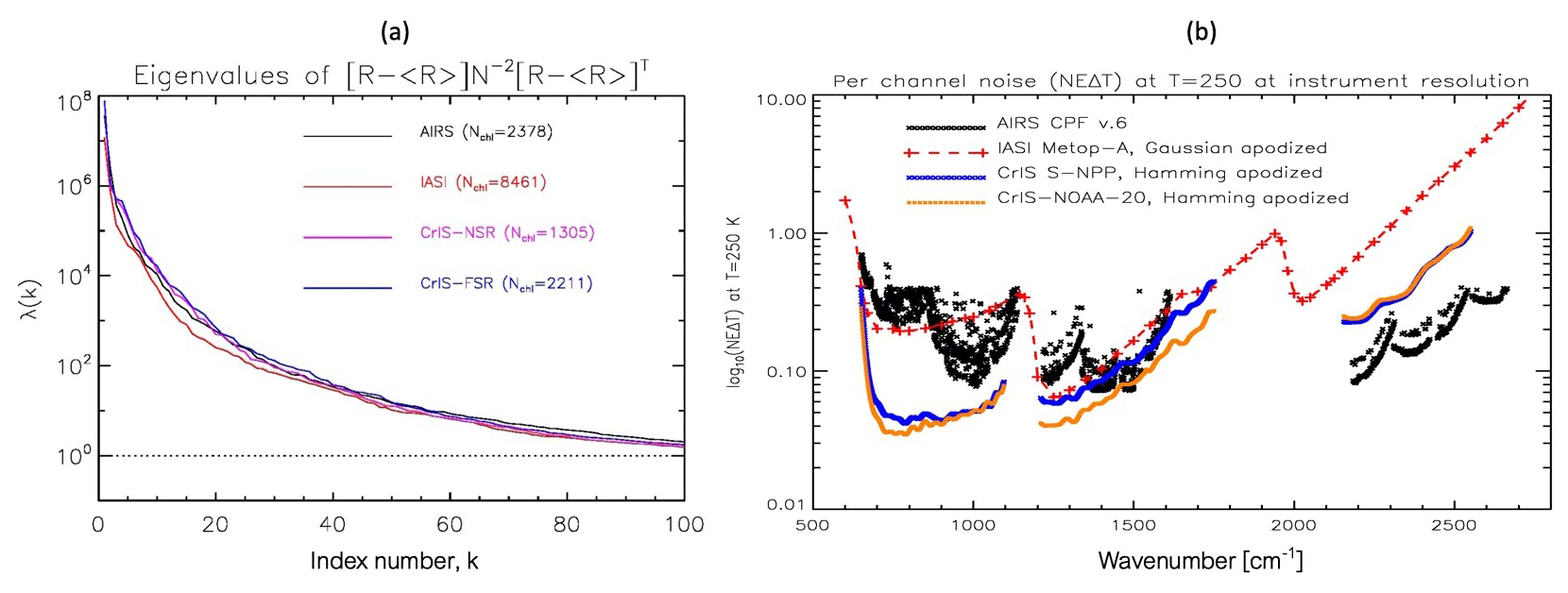
Figure 1 Information content analysis of four operational hyperspectral infrared instruments, AIRS (Atmospheric Infrared Sounder) in orbit on Aqua since 2002, IASI (Infrared Atmospheric Sounding Interferometer) in orbit on multiple MetOp platforms since 2006, and CrIS (Cross-track Infrared Sounder) in orbit on SNPP since 2011 and NOAA20 since 2017. We depict the SNPP CrIS in nominal-spectral-resolution (NSR) mode, with spectral resolution in its mid-wave and shortwave bands reduced to 1.25 and 2.5 cm⁻¹, respectively. NOAA20 CrIS is in full-spectral-resolution (FSR) mode with all spectral bands sampled at 0.625 cm⁻¹. (a) Eigenvector decomposition of the radiance covariance matrix as a measure of the information content in each instrument. The eigenvalues, λ, from an eigenvector decomposition of simulated radiances are plotted against the index number of each eigenvector, k. Information content is calculated as all eigenvalues λ>0. The total number of channels, N_chl, is listed in the figure legend. (b) Instrument noise, measured as the noise-equivalent delta temperature, NEΔT, for a scene with surface temperature equal to 250 K.

CLIMCAPS adopted the AIRS Science Team version 5 (v5) algorithm as its baseline retrieval method, which follows a sequential OE approach in solving the nonlinear inversion of infrared radiances into multiple distinct atmospheric variables (Maddy et al., 2009; Susskind et al., 2003). The inversion of top-of-atmosphere radiances is an ill-conditioned, under-determined, nonlinear problem that requires some form of stabilization to find a solution. In Bayesian (or probabilistic) OE systems, this is predominantly achieved with the introduction of an a priori (or background) estimate of the atmospheric state such that the solution is not an independent observation but instead represents an improvement on the background state given the top-of-atmosphere measurement of the true state (Rodgers, 1976, 1998, 2000).

The AIRS v5 system employed a linear regression as a priori for T, H₂O, and O₃ in the OE inversion step, which is generally referred to as a “physical” retrieval because it requires radiative transfer calculations, not regression correlation coefficients, to minimize the cost function at every scene. CLIMCAPS does not calculate a regression a priori for T, H₂O, and O₃ but instead uses a data assimilation product, specifically the Modern-Era Retrospective Analysis for Research and Applications version 2.0 (MERRA2; Gelaro et al., 2017; Molod et al., 2015). We argued in Smith and Barnet (2019) that a linear regression a priori amplifies instrument effects in the OE retrieval and thus hampers data continuity across platforms. Regression retrievals typically employ all spectral channels (Blackwell, 2005; Goldberg et al., 2003; Milstein and Blackwell, 2016; Smith et al., 2012) to retrieve atmospheric state variables simultaneously. If a regression retrieval is ingested as a priori then instrument artifacts can be propagated and even amplified in the retrieval product because OE uses the same spectral channels (albeit a subset) a second time. CLIMCAPS deliberately employs an instrument-independent a priori, i.e., MERRA2, for its T, H₂O, and O₃ retrievals to minimize instrument artifacts and promote data continuity across platforms. MERRA2 assimilates a small subset of IR channels (i.e., by selecting channels that are primarily sensitive to T but largely insensitive to H₂O, clouds, and trace gases) only sometimes (i.e., for clear-sky scenes only) and weighs them based on the time of measurement within the reanalysis window and with an assumed representation error across all scenes. This gives us confidence to argue that the IR channels used in CLIMCAPS rarely duplicate the information content of the IR channels used in MERRA2 at a specific scene. We argue that the IR information content from AIRS or CrIS in CLIMCAPS is much higher than in MERRA2 because CLIMCAPS retrieves the atmospheric state along the line of sight from a greater selection of cloud-cleared IR channels (i.e., all scenes except those with uniform cloud cover) and a full accounting of trace gas absorption. We contrast the CLIMCAPS a priori approach with those systems that employ a regression first guess such as AIRS v6 (Susskind et al., 2014) that runs a nonlinear regression using all IR channels to derive its a priori for T, H₂O, and O₃. Unlike AIRS v6, CLIMCAPS does not use the information content of IR channels twice because we designed it to minimize systematic instrument uncertainty and an aliasing of its retrieval null space error as a result. For the trace gas species, we adopted the same approach in CLIMCAPS as that used in AIRS v6 for CO, CO₂, HNO₃, N₂O, and SO₂ (AIRS Science Team/Joao Texeira, 2013). The CO climatology has no intra-annual variation but does vary seasonally and latitudinally, while the CO₂ climatology is a static value across all latitudes that increases annually according to a linear fit developed by Maddy (2007). The climatologies for the remaining trace gas species, HNO₃, N₂O, and SO₂, are static over time and space. The CLIMCAPS climatology for CH₄ is derived from a set of coefficients developed by Xiong et al. (2008, 2013) that is also used in the NOAA Unique Combined Atmospheric Processing System (NUCAPS).

The CLIMCAPS retrieval algorithm is outlined in Fig. 2, and we highlight four major steps here. (1) Local angle correction removes satellite view angle differences among a spatial cluster of 3×3 instrument footprints, also known as the “field of regard” or retrieval scene. (2) MW-only retrieval retrieves vertical profiles of T, H₂O, and liquid water path (LIQ), as well as surface emissivity (ε) using spectral channels from the microwave measurements (AMSU on Aqua, ATMS on SNPP and NOAA20). This results in an estimate of cloud-free vertical atmospheric structure in all but precipitating scenes. (3) Cloud clearing removes the radiative effects of clouds from hyperspectral IR channels in each field of regard using MW-only retrievals of LIQ and ε from step (2), profiles of T, H₂O, and O₃ from MERRA2, and climatologies of CO, CH₄, CO₂, HNO₃, N₂O, and SO₂. Cloud clearing is described in detail elsewhere (Smith, 1968; Chahine, 1974, 1977, 1982; Susskind et al., 2003) and remains one of the most robust approaches for the retrieval of atmospheric parameters within complex cloudy conditions and up to 90 % cloud cover. This step aggregates the cluster of 3×3 IR spectra into a single cloud-cleared IR spectrum from which all subsequent retrievals are done. In the case in which a scene has no cloud cover or IR channels are insensitive to clouds, the 3×3 cluster of IR channels is simply averaged. Note that cloud clearing reduces the spatial resolution of CrIS or AIRS footprints from ∼15 km instrument resolution at nadir to ∼50 km at nadir. (4) Stepwise OE retrieval sequentially retrieves surface temperature (T_s), ε, reflectivity (ρ), T, H₂O, and O₃, CO, CH₄, CO₂, HNO₃, N₂O, and SO₂. It is important to note that for cloud-cleared scenes, the profile retrievals do not represent conditions within the cloud fields but rather around or past the clouds. This is a subtle distinction, but it is meaningful in scientific studies and applications.

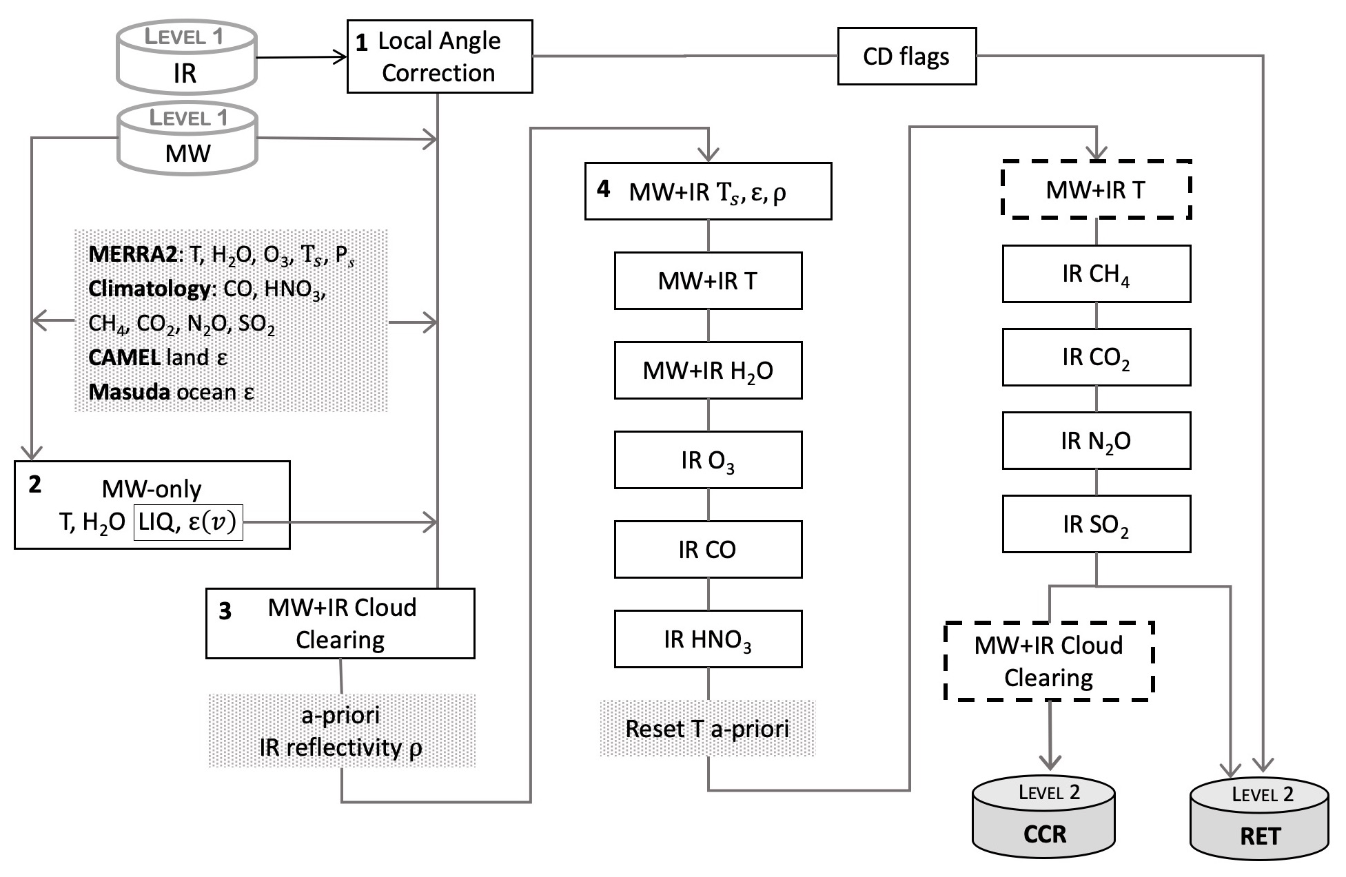
Figure 2 High-level abstraction of the CLIMCAPS retrieval method highlighting its stepwise optimal estimation (OE) retrieval. Steps 1 through 4 are discussed in the text. Boxes in grey indicate steps in which the a priori variables are defined. MERRA2 (GMAO, 2015) is the a priori for temperature (T), water vapor (H₂O), ozone (O₃), skin temperature (T_s), and surface pressure (P_s). We use the AIRS v6 climatologies for carbon monoxide (CO), carbon dioxide (CO₂), nitric acid (HNO₃), nitrous oxide (N₂O), and sulfur dioxide (SO₂) (AIRS Science Team/Joao Texeira, 2013); for methane (CH₄) the linear fit developed by Xiong et al. (2013) is used. The CLIMCAPS a priori for surface emissivity over land is based on the CAMEL database (Hook, 2019) and for ocean the Masuda model (Masuda et al., 1988) as modified by Wu and Smith (1997). The OE retrieval steps are listed in the order in which they appear in the code with MW+IR, indicating that the retrieval step depends on a subset of channels from both the microwave and infrared sounders, as well as infrared-only channels. Temperature and cloud-cleared radiances are retrieved twice, with the second step distinguished by dashed lines. Constituent detection (CD) flags indicate the presence of isoprene, ethane, propylene, and ammonia as calculated from single-field-of-view IR radiance channels.

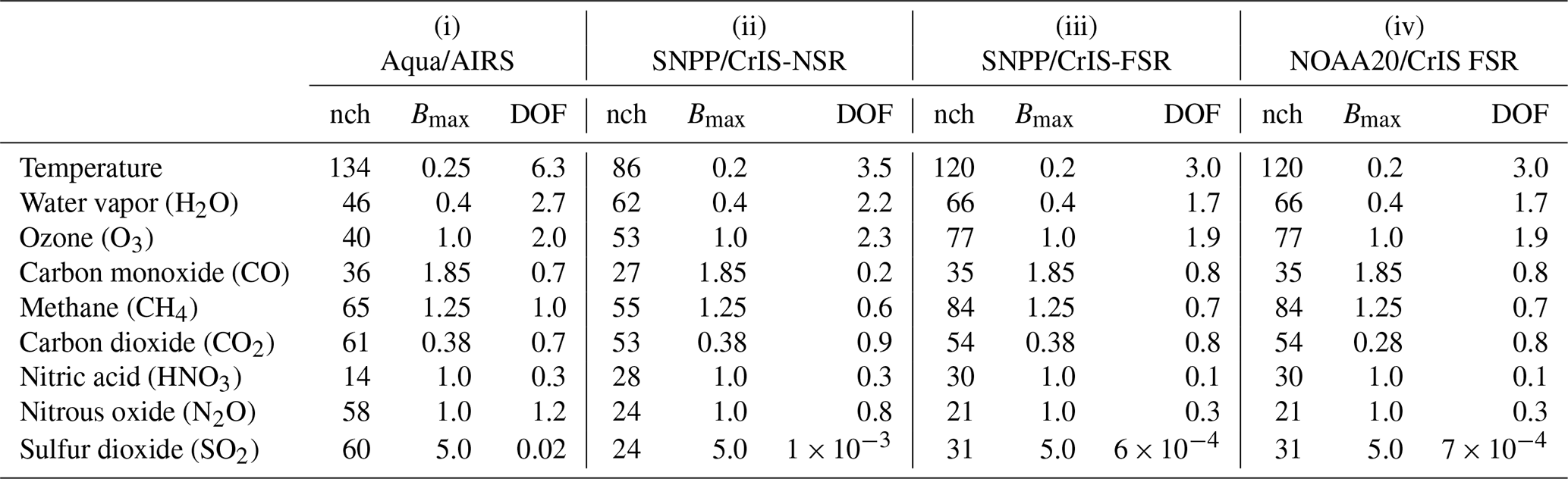
Each retrieval step (Fig. 2) is performed on a subset of channels with maximum sensitivity to the target variable and minimum sensitivity to all other variables. We adopted the channel selection method as described in Gambacorta and Barnet (2013). The channel sets for cloud clearing and all trace gases – O₃, CO, CH₄, CO₂, HNO₃, N₂O, and SO₂ – are selected from the IR measurements only, while the channel sets for surface parameters as well as atmospheric T and H₂O are selected from the IR and microwave measurements (MW+IR). The number of IR channels for each variable and each instrument is listed in Table 1 and represents the size, m, of the measurement vector, y, for each retrieval variable. While m varies among instruments and retrieval variables, the size, n, of the retrieval vector, x, remains constant at 100 vertical pressure levels (for temperature) and layers (for trace gas column densities) for the sake of accurate radiative transfer calculations. CLIMCAPS employs the stand-alone radiative transfer algorithm (Strow et al., 2003), originally developed for AIRS and later adopted for CrIS. Table 1 additionally lists two values: the maximum value (B_max) for each retrieval damping factor (i.e., a static scalar threshold below which spectral channels are damped according to their information content) and the degrees of freedom (DOFs) for the signal as the global average of CLIMCAPS cloud-cleared radiance spectra with m channels. We discuss the damping factor in Sect. 2.2 below, but in short, it determines the degree to which CLIMCAPS retains information from the radiance channels in the retrieved product.

Table 1 For each CLIMCAPS instrument and/or platform configuration, we list three parameters: the number of spectral channels (nch) used in the retrieval of temperature, H₂O, O₃, CO, CH₄, CO₂, HNO₃, N₂O, and SO₂; the damping factors applied as a regularization parameter (B_max); and degrees of freedom as a metric for vertically integrated observing capability. CLIMCAPS version 2.0 is configured for retrievals from (i) the Atmospheric Infrared Sounder (AIRS) on Aqua, (ii) the Cross-track Infrared Sounder in nominal-spectral-resolution mode (CrIS-NSR) on the Suomi National Polar-orbiting Partnership (SNPP) satellite, (iii) the CrIS in full-spectral-resolution mode (CrIS-FSR) on SNPP, and (iv) CrIS-FSR on NOAA20, the first of four Joint Polar Satellite Systems. The DOF values represent the mean from all ascending orbits (∼ 13:30 local overpass time) on 1 July 2018 from retrievals that were flagged as successful and rounded off to one decimal place.

2.2 CLIMCAPS averaging kernels

Rodgers (2000) defines averaging kernels as the sensitivity of the retrieved variable, $\widehat{\mathit{x}}$, to the true state of the variable, x, for a given moment in time and space. In its most basic form, an n×n AKM can be calculated for each retrieved variable as depicted in Eq. (1):

$$\begin{array}{}\text{(1)}& \mathbf{AKM}={\left[{\mathbf{K}}^{\mathbf{T}}{\mathbf{S}}_m^{-\mathrm{1}}\mathbf{K}+{\mathbf{S}}_{\mathrm{a}}^{-\mathrm{1}}\right]}^{-\mathrm{1}}{\mathbf{K}}^{\mathbf{T}}{\mathbf{S}}_m^{-\mathrm{1}}\mathbf{K},\end{array}$$

where K is the m×n matrix of weighting functions (or Jacobians) that characterizes measurement sensitivity to the a priori target variable as $\frac{\partial y}{\partial x_{\mathrm{a}}}$, S_m is a diagonal m×m matrix of instrument noise, and ${\mathbf{S}}_{\mathrm{a}}^{-\mathrm{1}}$ the regularization term, which in the Rodgers (2000) approach is defined by the inverse of an n×n a priori error covariance matrix, S_a. The value of S_a determines the amount of regularization applied to the retrieval step or the degree to which information content in the spectral measurement contributes to the final result. S_a has to be chosen carefully so that the information content of the retrieval (or regularized solution) can be optimized given the information content available in the measurement (von Clarmann and Grabowski, 2007).

In a Bayesian OE system, the regularization term determines how much the retrieved variable resembles the a priori variable. If S_a is low, then regularization is high and the measurement information content will be suppressed so that the retrieval more closely resembles the a priori. In most OE observing systems, it is computationally prohibitive to dynamically generate a scene-specific matrix, S_a, especially when data latency is a concern. Instead, a common approach is to set S_a to a static value that is calculated offline either as a statistical covariance of a data ensemble or a simple ad hoc assignment (Fu et al., 2016; Irion et al., 2018). S_a is then applied to each retrieval scene irrespective of the measurement information content for that scene. While this simplifies calculation, it risks suppressing information content when it is high or enhancing measurement uncertainty when information content is low. The Rodgers (2000) AKM (Eq. 1) can be described as a linear combination of measurement sensitivity weighted by uncertainty about the a priori state variable (S_a).

CLIMCAPS, in contrast, calculates an n×n AKM as in Eq. (2):

$$\begin{array}{}\text{(2)}& \mathbf{AKM}={\left[{\mathbf{K}}^{\mathbf{T}}{\mathbf{S}}_m^{-\mathrm{1}}\mathbf{K}+\mathit{\lambda }\right]}^{-\mathrm{1}}{\mathbf{K}}^{\mathbf{T}}{\mathbf{S}}_m^{-\mathrm{1}}\mathbf{K},\end{array}$$

with K the same as in Eq. (1), but S_m an m×m error covariance matrix that combines instrument noise with uncertainty from scene-specific and observing system effects as described by Smith and Barnet (2019). Moreover, the background error term, S_a in Eq. (1), is replaced here with λ, the damping factor listed in Table 1. This damping factor differs from S_a in two important ways: (i) unlike S_a, λ has horizontal variation because it is dynamically calculated for each retrieval scene based on the measurement information content for a target variable, and (ii) unlike S_a, λ has no vertical variation because it is a scalar value that assumes uniform uncertainty about the prior state, which can be an oversimplification in some cases. In contrast to Eq. (1), a CLIMCAPS AKM as in Eq. (2) can be described as the linear combination of measurement sensitivity weighted by known and propagated sources of uncertainty as well as scene-specific knowledge about measurement information content. While this is different from a traditional OE approach, both Eqs. (1) and (2) generate results that are within the observing system null space and thus part of the solution set of the ill-determined inversion problem.

CLIMCAPS adopted the AIRS v5 (Susskind et al., 2003, 2014) implementation of Eq. (2) (Maddy et al., 2009; Maddy and Barnet, 2008). Instead of an array size of n=100, CLIMCAPS calculates AKMs on a reduced set of pressure layers as defined by a series of overlapping trapezoidal functions. The thickness of each trapezoid layer is empirically determined from calculations of the vertical resolution of simulated measurements for each variable; e.g., CLIMCAPS has 31 trapezoid state functions for temperature and 9 for CO. These trapezoid state functions were selected by the AIRS Science Team, with approximately two trapezoids per retrievable layer quantity. CLIMCAPS employs these vertical trapezoid functions for a number of reasons: (i) they reduce the dimensionality of the Jacobian matrix to speed up algorithm processing time; (ii) compared to the 100 pressure layers needed for accurate radiative transfer calculation, the trapezoidal layers more closely resemble the true instrument vertical resolution calculated from simulated spectra for standard atmospheric state climatologies; and (iii) they act as a smoothing constraint and thus reduce the need for additional a priori stabilization factors. As mentioned, we use the Rodgers (2000) OE notation in this paper, but in practice the Jacobians in Eq. (2) are linearly transformed to the coarser trapezoidal grids using a transformation matrix W as follows: $\stackrel{\mathrm{̃}}{\mathbf{K}}=\mathbf{KW}$, making it a $m\times \stackrel{\mathrm{̃}}{n}$ matrix, with $\stackrel{\mathrm{̃}}{n}$ the number of trapezoid layers (see Maddy and Barnet, 2008, for more details).

Averaging kernels are unitless and typically range in value between 0.0 and 1.0, although they can sometimes have negative values for which the noise exceeds the signal (see Fig. 3 in Sect. 3 below). AKMs quantify CLIMCAPS observing capability at any given point in time and space because they account for all known sources of scene-specific and observing system uncertainty. They characterize a system's ability to observe a target variable at a specific scene. An alternative interpretation is that they quantify the degree to which the a priori variable compensates for the lack of observing capability at any specified scene (1.0−AKM). While CLIMCAPS AKMs do not measure retrieval accuracy (approximation to the truth), they do characterize retrieval uncertainty and information content. CLIMCAPS retrievals are not in situ measurements of the vertical atmospheric state, but under-determined nonlinear inverse measurements with a dependence on prior knowledge of the atmospheric state. In scientific analyses and operational applications, it is imperative that sounding observations are correctly interpreted lest their uncertainty be mistaken for measurement. CLIMCAPS AKMs characterize and quantify the weighted contribution from the measurement (0.0+AKM) and the a priori (1.0−AKM). An averaging kernel value of zero means that the measurement has no observing capability at that pressure layer and the solution will be the a priori. An averaging kernel value of unity means the measurement has 100 % observing capability and the solution will have no dependence on the a priori. In practice, however, averaging kernels range in value between these two endpoints such that $\mathrm{0.0}<\text{AKM}<\mathrm{1.0}$.

What can we learn about CLIMCAPS observing capability by diagnosing its AKMs? And how should we interpret differences between its retrievals from different parts of the globe or from different sounding systems? We can address these questions with a discussion of how each of the variables in Eq. (2) affects the AKMs. These are the Jacobians (K) that determine the structure of an AKM and the measurement error covariance matrix (S_m) with a regularization parameter (λ) that determines its magnitude.

CLIMCAPS Jacobians are finite-differencing (or brute-force) weighting functions that quantify the sensitivity of the calculated radiances to the a priori retrieval variable. They are m×n matrices, with m equal to the number of spectral channels in the retrieval subset (Table 1); out of 2211 CrIS channels, CLIMCAPS has m=120 selected for T and m=66 for H₂O. Jacobians are sensitive to the background state variables used in the forward radiative transfer calculation. This is the only parameter in Eq. (2) that ingests a priori information. If an a priori is biased with respect to the true background state, the same bias will propagate into the Jacobians. For example, if the CO a priori is a climatology of a typical source site, then the Jacobian will indicate high measurement sensitivity because high concentrations of mid-tropospheric CO result in strong absorption lines in the calculated radiance and thus yield large weighting functions. If such weighting functions are applied to a retrieval for which the scene-specific CO concentrations are low, then the averaging kernels will mistakenly indicate high observing capability to CO at that scene, which risks representing the uncertainty as a signal unless the averaging kernels are adjusted according to known sources of uncertainty.

Clouds are one of the primary sources of scene-specific uncertainty. While CLIMCAPS requires no knowledge about the a priori state of clouds, it calculates radiance uncertainty due to clouds in the cloud clearing step (Table 1). Cloud clearing uncertainty, together with uncertainty from other state variables, is propagated into the measurement error covariance matrix, S_m, according to the method described in Smith and Barnet (2019). If a scene has high uncertainty due to clouds, S_m will increase and AKM will decrease to reflect a reduced observing capability. Scene-dependent cloud effects are therefore not explicitly accounted for in AKMs through radiative transfer calculation, but their scene-dependent uncertainty is derived and propagated into one of the error terms.

CLIMCAPS performs singular value decomposition (SVD) of the matrix ${\stackrel{\mathrm{̃}}{\mathbf{K}}}^T{\mathbf{S}}_m^{-\mathrm{1}}\stackrel{\mathrm{̃}}{\mathbf{K}}$ to derive a set of scene-specific eigenvectors for use in the retrieval. We refer to this $\stackrel{\mathrm{̃}}{n}\times \stackrel{\mathrm{̃}}{n}$ eigenvector matrix as $\stackrel{\mathrm{‾}}{\stackrel{\mathrm{‾}}{\mathbf{K}}}$, with eigenvalues, λ_i, on its diagonal. SVD benefits the retrieval in that it minimizes (maximizes) the a priori contribution when measurement information content is high (low) such that the retrieval product deviates from its a priori only when the radiance measurement has information content. According to Eq. (2), the regularization term is derived from the eigenvalues and determines the degree to which these eigenvectors are damped in the solution according to the critical threshold, λ_c, which is derived from B_max (Table 1) such that ${\mathit{\lambda }}_{\mathrm{c}}={\left(B_{\max }\right)}^{-\mathrm{2}}$. B_max is a scalar value, empirically determined offline, and defines the maximum allowable noise that can propagate into the retrieval. We illustrate how this works in practice with the example discussed below.

Table 2 Example of eigenvalues and damping factors for a hypothetical temperature retrieval.

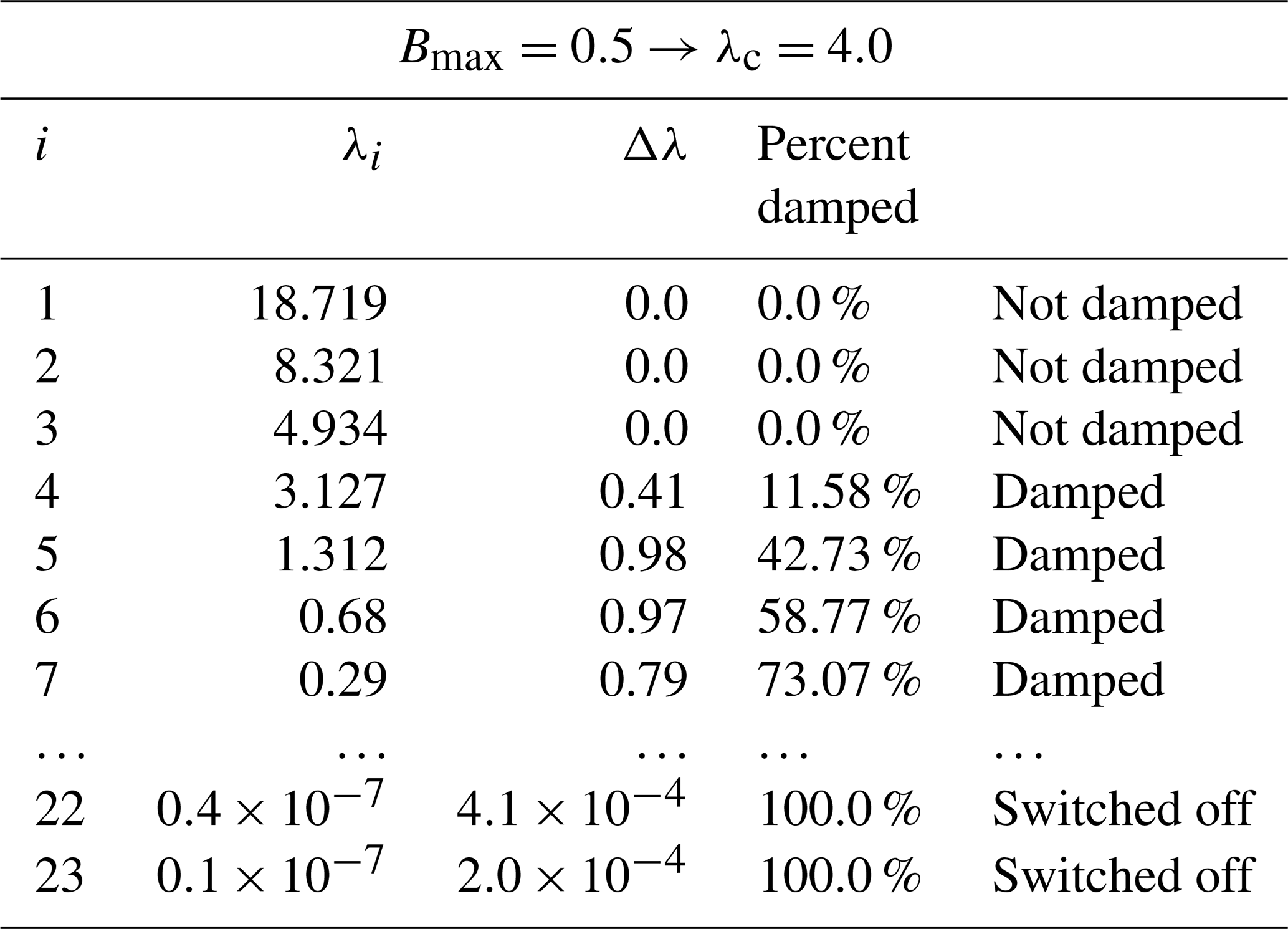
In Table 2, the $\stackrel{\mathrm{‾}}{\stackrel{\mathrm{‾}}{\mathbf{K}}}$ matrix for temperature has five significant eigenvalues (i.e., where λ_i≥1.0), which means that the observing system has five independent pieces of information and can solve for temperature at five distinct pressure levels. For a B_max=0.5, λ_c=4.0. All eigenvectors with λ_i>λ_c will contribute to the retrieval undamped. In Table 1, we see that the first three eigenvectors will thus contribute 100 % of their information to the retrieval. Those eigenvectors with ${\mathit{\lambda }}_{\mathrm{c}}>{\mathit{\lambda }}_i>\mathrm{0.05}$ will be fractionally damped as follows: $\mathrm{1.0}-\frac{{\mathit{\lambda }}_i}{({\mathit{\lambda }}_i+\mathrm{\Delta }\mathit{\lambda })}$, where $\mathrm{\Delta }\mathit{\lambda }=\sqrt{{\mathit{\lambda }}_{\mathrm{c}}}\sqrt{{\mathit{\lambda }}_i}-{\mathit{\lambda }}_i$. Accordingly, the fourth eigenvector (Table 2) will be 11.58 % damped, the fifth 42.73 %, and so on. Those eigenvectors with λ_i<0.05 will be switched off so that they make no contribution to the retrieval because they are regarded as sources of noise. An observing system can be over-damped in which case it does not let enough functions contribute 100 % of their information. Such a system would suppress the amount of information contributed by the measurements and force a strong dependence on the a priori. Alternatively, a system can be under-damped in which case too many functions contribute to the retrieval undamped such that the measurements contribute not only information (eigenvectors with λ_i≥1.0) but also noise (eigenvectors with λ_i<1.0). CLIMCAPS-Aqua has B_max=0.25 and CLIMCAPS-NOAA20 B_max=0.20 (Table 1), which translates to λ_c=16.0 and λ_c=25.0, respectively. In our example given in Table 2, CLIMCAPS-Aqua will leave only the first eigenvector undamped, while CLIMCAPS-NOAA20 will not let a single eigenvector contribute 100 % of its information but damp all of them.

We adopt this type of regularization in CLIMCAPS because we do not know with absolute certainty that we fully accounted for all sources of uncertainty in the S_m matrix. With this approach, we can account for those sources of uncertainty not explicitly characterized in previous retrieval steps (Fig. 1). In an ideal system in which all sources of uncertainty are fully characterized, all eigenvectors with λ_i≥1.0 should typically contribute to the retrieval undamped.

3 Results and discussion

In this section, we use AKMs to diagnose CLIMCAPS observing capability (or sensitivity to the true state) for CLIMCAPS-Aqua and CLIMCAPS-NOAA20 using two global days of retrievals, 1 July and 15 December 2018. AKMs quantify the potential each measurement has to resolve the atmospheric state given observing system characteristics and prevailing conditions at the retrieval scene. So far, we have referred to the AKM associated with each retrieval. Here we take a look at the individual averaging kernels (or rows) of each AKM and specifically distinguish the diagonal of the AKM (or AKD) as a vector representation of the maximum sensitivity at each pressure level.

3.1 Diagnosing CLIMCAPS observing capability

Figure 3 depicts the averaging kernels for T and H₂O from CLIMCAPS-NOAA20 for five different retrieval scenes within a few hundred miles of each other south of South Africa where the Atlantic and Indian oceans converge. The peak of each kernel depicts the atmospheric pressure level at which observing capability is strongest. The spread of an averaging kernel, quantified as the full-width at half-maximum (FWHM), can be interpreted as the vertical resolution of information content at its peak pressure. Accordingly, we see here that CLIMCAPS has higher vertical resolution (smaller FWHM) for T in the lower troposphere (Fig. 3; top row) compared to the stratosphere but in turn a stronger observing capability for T in the stratosphere (larger peak values). The vertical resolution for H₂O (Fig. 3; bottom row) is fairly consistent throughout the troposphere, but we see how observing capability varies strongly from scene to scene. Note how the kernels fall below zero at times. For scenes 1 and 3 (47.8^∘ S, 29.4^∘ E and 41.7^∘ S, 22.6^∘ E, respectively) the kernels for both T and H₂O are generally low in the troposphere compared to other scenes. This means the observing capability of CLIMCAPS-NOAA20 is weak and only a small amount of measured information will be added to the a priori at those scenes. Scene 4 (36.6^∘ S, 29.9^∘ E), on the other hand, has higher kernel peaks and CLIMCAPS-NOAA20 thus has a stronger capability to retrieve atmospheric structure in the troposphere and add new information to prior state variables at that scene.

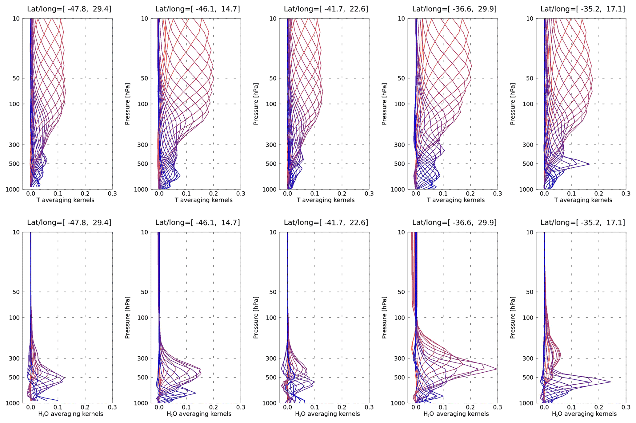
Figure 3 Scene dependence of CLIMCAPS-NOAA20 averaging kernels for coincident (top row) temperature (T) and (bottom row) water vapor (H₂O) retrievals at five scenes (left to right) on 1 July 2018. The latitude–longitude coordinates are listed at the top of each figure. Averaging kernels (Eq. 2) quantify and characterize the signal-to-noise ratio of an observing system and are affected by the scene-dependent effects (e.g., temperature lapse rate, amount of gas molecules, surface emissivity, and cloud uncertainty) as much as the measurement characteristics (e.g., spectral resolution, instrument calibration, and noise). CLIMCAPS retrieves T and H₂O sequentially each with a unique subset of channels, which means that the variations in these averaging kernels are independent of each other.

Figure 4 presents the averaging kernels for seven CLIMCAPS-NOAA20 retrieval parameters. They are (left to right) T, H₂O, O₃, CO, CH₄, CO₂, and HNO₃. These kernels represent the average for all northern midlatitude scenes (30–60^∘ N, 180^∘ W–180^∘ E) on 1 July 2018, hence their smooth appearance compared to those in Fig. 3 for individual scenes. We see how retrieval sensitivity to the true state depends strongly on the target variable. CLIMCAPS retrieves each state variable using a subset of spectral channels (Table 1) selected to have a high degree of sensitivity for the target variable and low sensitivity to all other atmospheric state variables radiatively active in the same spectral region (Gambacorta and Barnet, 2013). The CLIMCAPS sequential OE approach, with channel selection and uncertainty propagation, minimizes spectral correlation in the retrieved variables (Smith and Barnet, 2019). This means that any correlation that does exist can mostly be attributed to geophysical, not observing system, effects. On average, CLIMCAPS-NOAA20 has distinct stratospheric and tropospheric sensitivity to the true states of T, O₃, and CO₂. For H₂O, CO, and CH₄, CLIMCAPS-NOAA20 observing capability is limited to the mid-troposphere (200–700 hPa). Unlike CO and CH₄, the kernels for H₂O have peaks at multiple layers and varying degrees of vertical resolution (FWHM). On average in the summertime northern midlatitude zone, CLIMCAPS-NOAA20 has barely any sensitivity to HNO₃ and very little to CO₂ below 500 hPa.

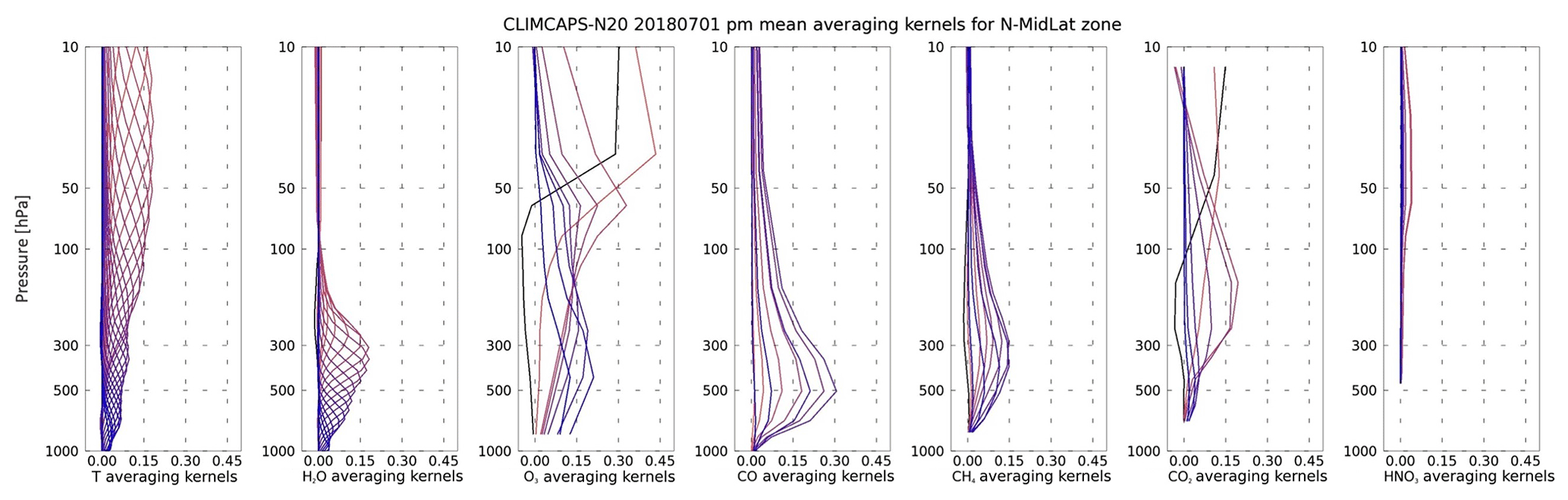
Figure 4 The mean of a set of averaging kernels for seven CLIMCAPS-NOAA20 ascending orbit retrieval variables across the northern midlatitude zone (30 to 60^∘ N) for a global day of daytime (ascending orbit) observations from NOAA20 on 1 July 2018. From left to right is air temperature (T), water vapor (H₂O), ozone (O₃), carbon monoxide (CO), methane (CH₄), carbon dioxide (CO₂), and nitric acid (HNO₃). CLIMCAPS calculates 31 averaging kernels for T, 22 for H₂O, 10 for O₃, CO, and HNO₃, 11 for CH₄, and 9 for CO₂. The averaging kernels for T, H₂O, and CO are defined on layers from the top of the atmosphere to the sea surface, with those for O₃ extending down to 822 hPa, CH₄ down to 800 hPa, CO₂ down to 700 hPa, and HNO₃ down to 450 hPa.

To simplify comparison across multiple latitudinal zones and retrieval systems, we use averaging kernel matrix diagonal vectors (in short, AKDs from here on) to summarize the maximum sensitivity at each pressure layer. The trace of the AKM (sum of AKD) defines the degrees of freedom (DOFs) for the signal or the CLIMCAPS information content about the vertical state of a target variable. DOF can be smaller than the number of significant eigenvectors due to damping (Eq. 2) and can be interpreted as the SNR of a retrieval system.

In Fig. 5, we contrast the AKDs for five latitudinal zones – south polar (90 to 60^∘ S), southern midlatitude (60 to 30^∘ S), tropics (30^∘ S to 30^∘ N), northern midlatitude (30 to 60^∘ N), and north polar (60 to 90^∘ N) – on 15 December 2018 for CLIMCAPS-NOAA20 (top panel) and CLIMCAPS-Aqua (bottom panel). We observe distinct latitudinal variation in CLIMCAPS-NOAA20 for H₂O, O₃, and CO₂. In contrast, CLIMCAPS-Aqua information content has latitudinal variability for T, H₂O, O₃, and HNO₃. For CO and CH₄, CLIMCAPS-NOAA20 and CLIMCAPS-Aqua information content is similar in magnitude and structure with mid-tropospheric peaks at 500 and 400 hPa, respectively. Notice the marked differences in T and H₂O AKDs between CLIMCAPS-Aqua and CLIMCAPS-NOAA20 (Fig. 5, two left panels). Compared to CLIMCAPS-NOAA20, CLIMCAPS-Aqua has higher observing capability for atmospheric structure in the mid-troposphere; its T and H₂O retrievals have smaller dependence on the a priori with a larger contribution of information by the AIRS/AMSU spectral channels. Both observing systems use the same a priori, namely MERRA2, and they measure conditions on the same day. While Aqua and NOAA20 both have 13:30 local overpass times, their orbits are not aligned and they view the same scene at different view angles almost an hour apart. Cloud structure and amount can change significantly in that time. But even if the cloud fields remained unchanged over a few hours, measurement uncertainty due to clouds can be different at nadir (looking down at clouds) than at the edge of a scan (looking at clouds with an angle). Smith et al. (2015) discussed how observing capability changes due to instrument effects – spectrometers (AIRS) versus interferometers (CrIS) – in cloudy scenes. While the information content for an ensemble of simulated AIRS and CrIS measurements is similar (Fig. 1), differences in their spectral resolution, detector arrays, and algorithm channel sets introduce variation in the information content of their measurements at a specific same scene. CLIMCAPS-Aqua uses 134 and 46 channels for T and H₂O, while CLIMCAPS-NOAA20 uses 120 and 66 for the same variables, respectively. Moreover, the damping factor for CLIMCAPS-Aqua T is lower than that for CLIMCAPS-NOAA20.

We designed and implemented CLIMCAPS to be similar for all instruments and platforms with the goal that its sounding record can be continuous over decades despite changes in technology. Global ensembles of T and H₂O retrievals from both systems – CLIMCAPS-NOAA20 and CLIMCAPS-Aqua – display similar root mean square statistics (not shown) when compared to ECMWF (European Centre for Medium-Range Weather Forecasts) reanalysis fields. We have found that CLIMCAPS-NOAA20 and CLIMCAPS-Aqua have similar observing capabilities for the trace gases, but compared to CLIMCAPS-Aqua, CLIMCAPS-NOAA20 appears over-damped; its T and H₂O retrievals have low sensitivity to the true state. This is reflected in the CLIMCAPS regularization threshold for T from CrIS/ATMS on SNPP and NOAA20 that is lower than that for AIRS/AMSU on Aqua (Table 1). This threshold was first developed for nominal-spectral-resolution CrIS (measurements available at launch in 2011) and never updated when full-spectral-resolution CrIS measurements became available 2 years later. In the future, we will experiment with these threshold values to test if we can achieve consistency in averaging kernels across CLIMCAPS-Aqua, CLIMCAPS-NOAA20, and CLIMCAPS-SNPP. We are interested in addressing the question of whether we can achieve continuity in information content despite instrument differences. The disparity in information content we currently observe between CLIMCAPS-Aqua and CLIMCAPS-NOAA20 (Fig. 5) tells us that the two systems apply different weighting to the radiance measurements and thus vary in their dependence on the a priori. This can introduce inconsistencies in the data record and hamper continuity. In using averaging kernels as a metric, we can evaluate information content under similar conditions across CLIMCAPS-Aqua, CLIMCAPS-NOAA20, and CLIMCAPS-SNPP and thus test for continuity in their observing capability.

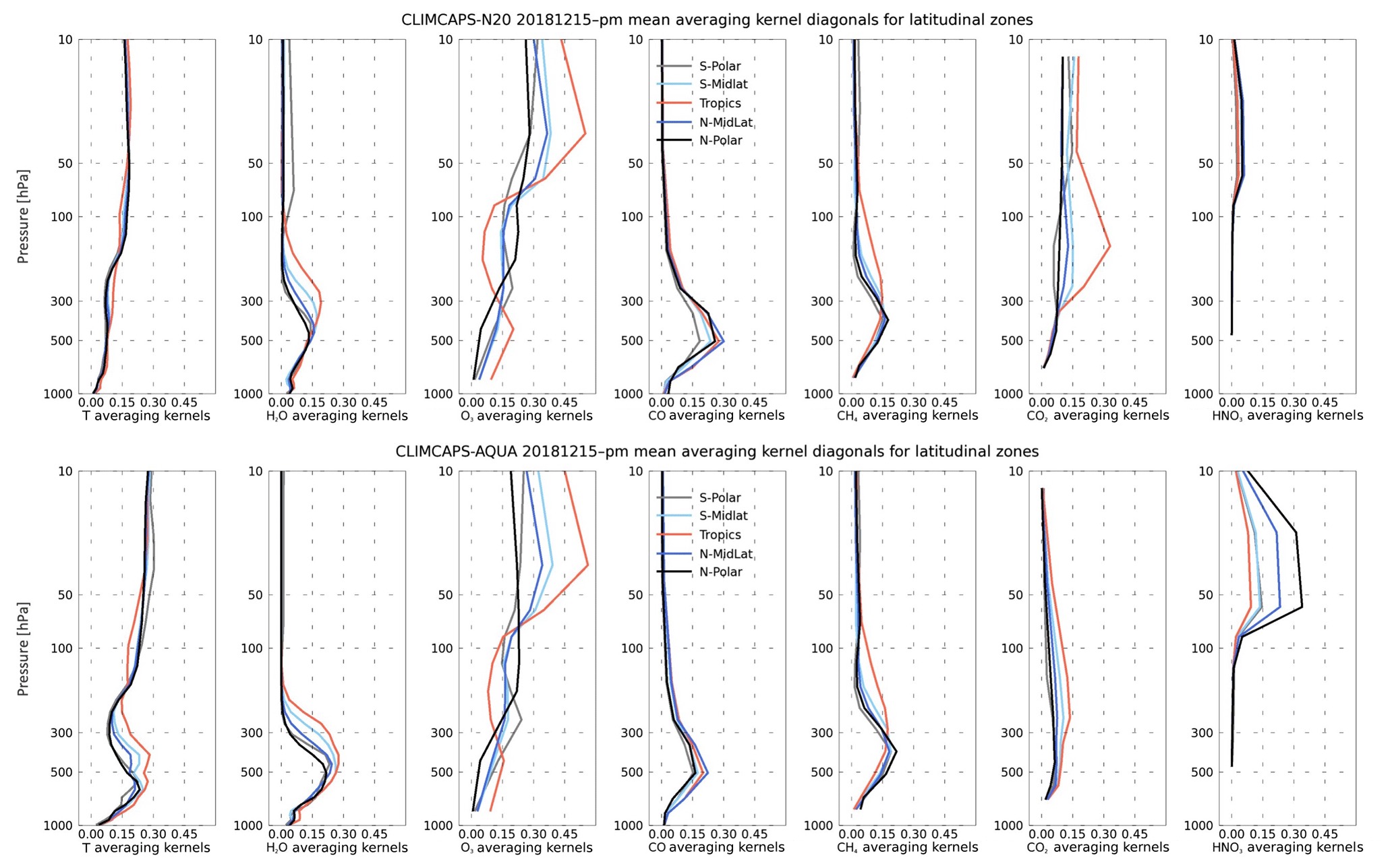
Figure 5 Averaging kernel diagonal vectors for seven retrieval variables – (left to right) T, H₂O, O₃, CO, CH₄, CO₂, and HNO₃ – from (top) CLIMCAPS-NOAA20 and (bottom) CLIMCAPS-Aqua ascending orbits on 15 December 2018. For each observing system, the mean of the diagonal vector is calculated across five latitudinal zones – south polar (90 to 60^∘ S), southern midlatitude (60 to 30^∘ S), tropics (30^∘ S to 30^∘ N), northern midlatitude (30 to 60^∘ N), and north polar (60 to 90^∘ N).

Figure 6 maps CLIMCAPS-NOAA20 DOF for T, H₂O, CO, and O₃ on 15 December 2018. CLIMCAPS AKMs are independent of the final retrieved variable and thus independent of whether the solution converges or not. We therefore do not apply a quality control filter that introduces data gaps other than those introduced by orbital tracks at low latitudes. Note how the spatial patterns of DOF for the four variables are largely independent of each other. This stems from the fact that CLIMCAPS uses channel subsets and uncertainty propagation to minimize spectral correlation across retrieval variables (Smith and Barnet, 2019). Where DOF patterns do have distinct features, such as the low O₃ DOF feature over Canada (Fig. 6d), we can understand it by evaluating the physical state to determine if it is due to conditions such as low O₃ concentrations, low lapse rates, or stratospheric warming. All retrieval variables and their uncertainty metrics are coincident in space and time in the CLIMCAPS product files to facilitate these types of analyses.

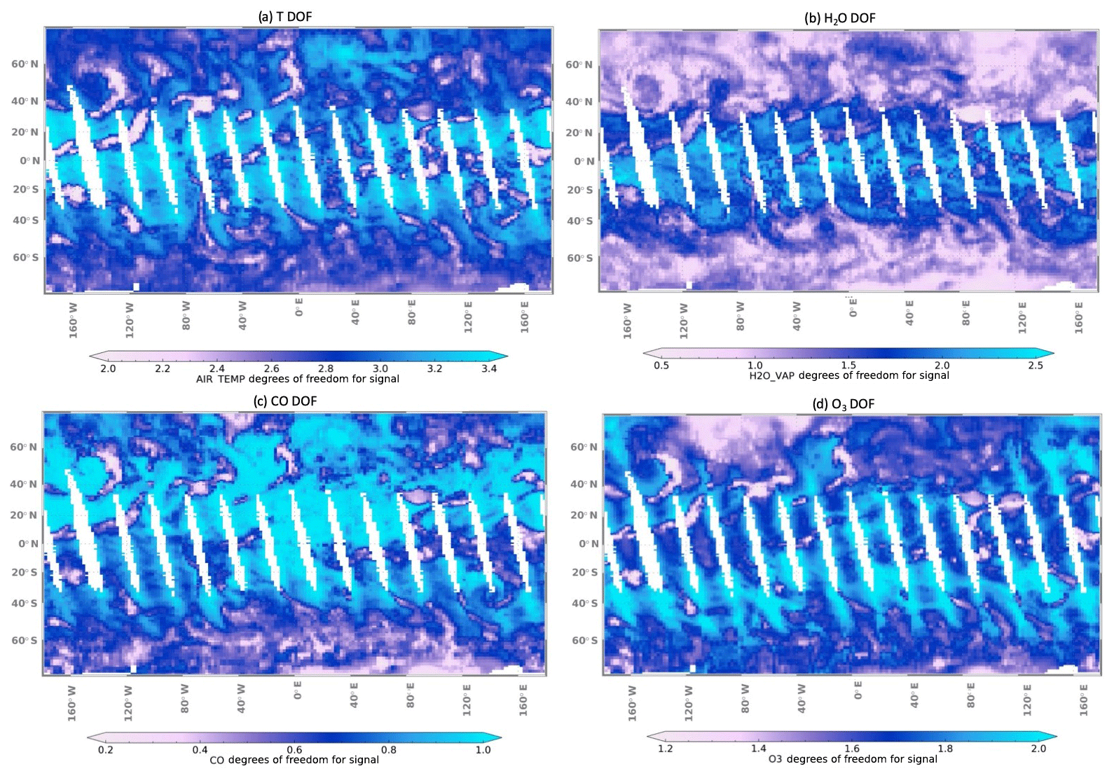
Figure 6 Spatial variation in the degrees of freedom (DOFs) for the signal for four retrievals from CLIMCAPS-NOAA20 ascending orbit on 15 December 2018: (a) temperature (T), (b) water vapor (H₂O), (c) carbon monoxide (CO), and (d) ozone (O₃). Note how the spatial patterns in DOFs for each retrieval variable are largely independent of the others.

While CLIMCAPS observing capabilities for these variables are largely independent of each other, their spatial patterns do all display a sensitivity to clouds in the lower latitudes. We see similar patterns in cloud cover from satellite imagery of the same day (not shown). AKMs do not directly ingest any information about the background atmospheric state or the a priori retrieval variable. Nor do the AKMs ingest any cloud variables in radiative transfer calculations for deriving the K matrix. Any knowledge about clouds that does exist in the AKMs (and derived DOF) is from the cloud uncertainty that is quantified during the cloud clearing step and propagated through to the S_m matrix. If cloud uncertainty is high, S_m will increase and DOF will decrease according to Eq. (2). This is why we see lower values for DOF in cloudy and overcast scenes.

Figure 7 illustrates the degree to which AKDs vary across a northern midlatitude zone (30 to 60^∘ N) for seven retrieval variables; from left to right they are T, H₂O, O₃, CO, CH₄, CO₂, and HNO₃. The solid lines represent their mean AKDs, with the error bars quantifying their variation about the mean. The degree to which the AKDs vary across space, pressure, variables, and instruments in Fig. 7 is also the degree to which CLIMCAPS observing capability varies. Overall, CLIMCAPS-Aqua variation for T and H₂O is significantly higher than that for CLIMCAPS-NOAA20. Given that T is retrieved from CO₂-sensitive infrared channels, note how CLIMCAPS-NOAA20 AKD for T has insignificant vertical variation across this latitudinal zone, with an absence of a distinct peak in the troposphere, but its AKD for CO₂ not only has high variability but also a distinct peak in the upper troposphere. CLIMCAPS-Aqua, on the other hand, has T AKDs with high variability and a distinct tropospheric peak, but its CO₂ AKDs have no distinct peak and low vertical variability. This suggests that observing capability for CO₂ is enhanced (depressed) when observing capability for T is depressed (enhanced). Two other variables that are spectrally correlated are H₂O and CH₄. The channels sensitive to CH₄ absorption are also sensitive to H₂O. CLIMCAPS minimizes their correlation in the final retrieval products through channel selection for spectral purity coupled with a sequential propagation of scene-dependent uncertainty, but a degree of correlation persists as seen in Fig. 7. We see this in CLIMCAPS-NOAA20 observing capability that is lower for both H₂O and CH₄, while in CLIMCAPS-Aqua it is higher for both variables.

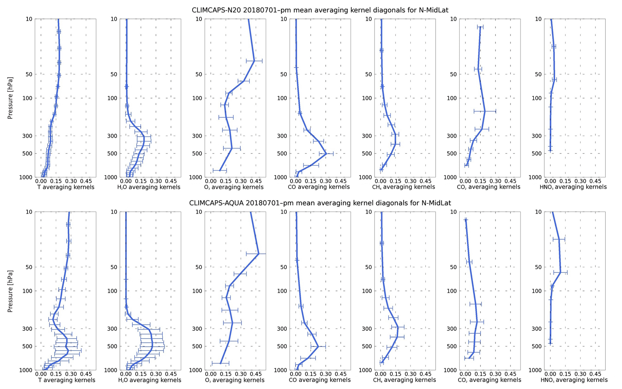
Figure 7 The mean (blue line) and standard deviation (blue error bars) of averaging kernel matrix diagonals in the northern midlatitude zone (30 to 60^∘ N) on 1 July 2018 from (top) CLIMCAPS-NOAA20 and (bottom) CLIMCAPS-Aqua, both ascending orbits. The error bars indicate the degree to which the averaging kernel diagonals vary spatially across the latitudinal zonal.

3.2 Averaging kernels in data intercomparison studies

Data assimilation models typically use infrared radiance channels to assimilate T and H₂O, but for trace gases they use the retrieved profiles (Levelt et al., 1998; Clerbaux et al., 2001; Yudin, 2004; Segers et al., 2005; Pierce et al., 2009; Liu et al., 2012). Top-of-atmosphere radiances are highly correlated, highly mixed signals of atmospheric variables. A single channel in the ∼2100 cm⁻¹ spectral range may contain information about CO, but it also contains information about N₂O, T, surface emissivity, surface temperature, and H₂O. If a model wants to assimilate CO spectral channels then it would have to account for all interfering species in addition to the uncertainty of CO, lest it introduce bias in its characterization of CO processes. This has proven prohibitively difficult in the case of trace gases for which the target variable has a weak spectral signal with interference from variables with much stronger signals. Instead, modellers rely on retrieval algorithms to decompose the infrared channels into distinct trace gas species. Maddy and Barnet (2008) gave a detailed description of how AKDs can be used together with the retrieved profiles to remove a priori information from the retrieval and thus facilitate their assimilation at a minimum cost to the model. Today, the Maddy–Barnet method is well established and widely used as the standard method for data assimilation of retrieved trace gas profiles (Pierce et al., 2009).

In this section, we turn our attention to the value of AKMs in data intercomparison studies, specifically the intercomparison of different remote sounding products, all with their own sets of AKMs. What can we learn about a retrieval product from its AKMs, and how can this facilitate understanding and interpretation?

Figure 8 illustrates CLIMCAPS-NOAA20 O₃ retrieval diagnostics at three different scenes in the Northern Hemisphere on 1 July 2018. For each scene, the diagnostics are (i) the O₃ averaging kernels and (ii) the departure from the a priori (retrieval minus a priori). The former characterizes CLIMCAPS observing capability for O₃ at that scene, and the latter quantifies the changes made to the a priori given the measurement information content in the CLIMCAPS channel subset. Recall that CLIMCAPS employs MERRA2 as a priori for T, H₂O, and O₃ (Smith and Barnet, 2019). MERRA2 assimilates partial column ozone from a series of solar backscatter ultraviolet (SBUV) instruments between 1980 and September 2004. After September 2004, SBUV data are replaced by total ozone retrievals from the Ozone Monitoring Instrument (OMI) and stratospheric ozone profiles from MLS (Levelt et al., 1998) onboard the NASA Aura satellite. Wargan et al. (2017) validated MERRA2 ozone against ozonesondes and found them to give an accurate representation of cross-tropopause gradients and variability on daily and interannual timescales. MERRA2 does not assimilate any infrared channels or retrievals from CrIS or AIRS for its O₃ product. Figure 8 illustrates that CLIMCAPS has observing capability for stratospheric and tropospheric ozone, which means it has the potential to add new information to the MERRA2 a priori fields in two distinct parts of the atmosphere. While CLIMCAPS-NOAA20 observing capability is similar at all three scenes, we see that the retrieval deviation from the a priori (black line) varies significantly from scene to scene. In scene (a), CLIMCAPS-NOAA20 increased the stratospheric concentrations while decreasing tropospheric O₃. In scene (b), CLIMCAPS-NOAA20 mainly reproduced MERRA2 tropospheric O₃ while increasing it slightly in the lower stratosphere. In scene (c), CLIMCAPS-NOAA20 added no new information to MERRA2 stratospheric O₃, but it increased its upper tropospheric concentrations.

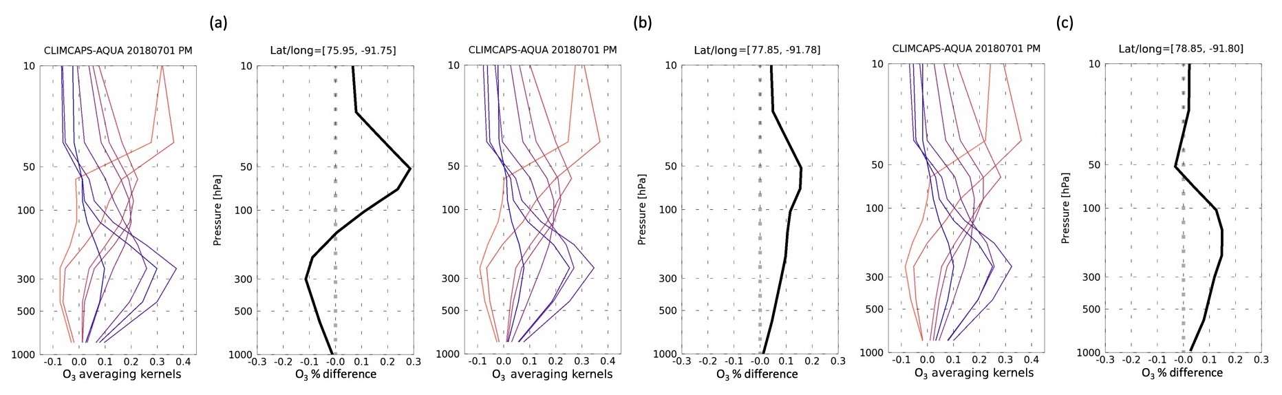
Figure 8 An evaluation of ozone (O₃) retrievals from CLIMCAPS-NOAA20 ascending orbit on 1 July 2018 for three scenes at (a) 76.0^∘ N, 91.8^∘ W; (b) 77.9^∘ N, 91.8^∘ W; and (c) 78.9^∘ N, 91.8^∘ W. For each scene, the averaging kernels are displayed on the left and the retrieval departure from a priori on the right. CLIMCAPS uses MERRA2 as a priori for O₃. Scenes with averaging kernels similar in structure can have an a priori departure that varies in structure. All three scenes presented here passed CLIMCAPS quality control and are labeled “successful”. For each scene, CLIMCAPS additionally derives uncertainty metrics about the presence of clouds and we list them here. Scene (a) has a cloud fraction (CF) of 1 %, cloud-top pressure (CTP) of 425 hPa, cloud clearing uncertainty (CC_unc) of 0.29, and cloud clearing error (CC_err) of 0.5. Scene (b) has CF=1 %, CTP=273 hPa, CC_unc=0.29, and CC_err=0.5. Scene (c) has CF=3 %, CTP=375 hPa, CC_unc=0.33, and CC_err=0.76.

What does it mean when the AKMs show strong observing capability but the retrieval hardly deviates from the a priori? We interpret this as the CLIMCAPS CrIS IR channel set for O₃ largely confirming the MERRA2 O₃ profile at that scene. Aside from water vapor, ozone is the only trace gas variable in CLIMCAPS that uses an a priori with space–time structure. All other gases – CO, CO₂, CH₄, N₂O, and HNO₃ – use climatologies with limited to no spatial variation as discussed in Sect. 2.1. Any space–time structure thus visible in the retrievals of these gas species originates from the information content in the IR channels only.

For the same day, Fig. 9 illustrates CLIMCAPS-NOAA20 temperature retrieval diagnostics for three cloudy scenes in the Southern Hemisphere. Again, we note how the system has similar observing capabilities at each scene, but the retrieval departure from MERRA2 varies significantly. Note how CLIMCAPS-NOAA20 increases MERRA2 temperature at all scenes in the lower stratosphere and troposphere but decreases MERRA2 temperature in the upper stratosphere. MERRA2 does assimilate CrIS and AIRS IR radiance channels that are sensitive to temperature. We argue, however, that on a scene-by-scene basis it is highly improbable that CLIMCAPS uses IR measurements twice (first as assimilated information in MERRA2, second as a measurement vector in OE retrievals) due to the strong spectral and spatial filters adopted in data assimilation systems. Even when a MERRA2 grid cell does contain IR information at a target CLIMCAPS footprint, we consider the impact of the assimilated IR channels on the OE retrieval to be negligible. CLIMCAPS aggregates an array of 3×3 fields of view (∼14 km) during cloud clearing (step 3 in Fig. 2) and retrieves all subsequent variables from the cloud-cleared radiance that represents the clear portion of partly cloudy atmospheres on a larger field of regard (∼50 km). MERRA2, on the other hand, assimilates single-field-of-view radiances for clear-sky atmospheres. MERRA2 assimilates measurements from many sources, so the contribution made by a single source at a target site is low, especially considering that each source is weighed according to a static, predetermined representation error. CLIMCAPS, on the other hand, uses cloud-cleared IR radiances as one of its primary sources of information that it weighs based on scene-specific information content analysis.

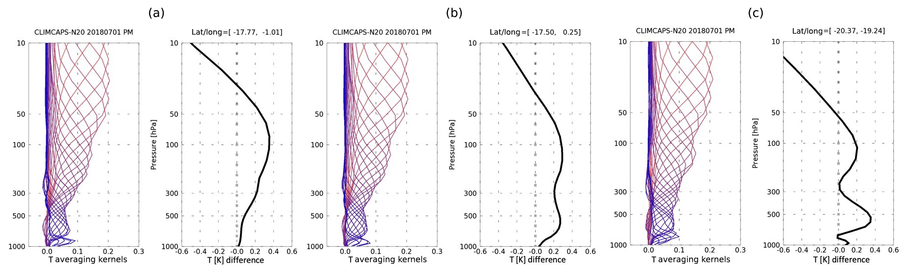
Figure 9 An evaluation of temperature (T) retrievals from CLIMCAPS-NOAA20 ascending orbit on 1 July 2018 for three scenes at (a) 17.8^∘ S, 1.0^∘ W; (b) 17.5^∘ S, 0.25^∘ E; and (c) 20.4^∘ S, 12.2^∘ W. For each scene, the averaging kernels are displayed on the left and the retrieval departure from a priori on the right. CLIMCAPS uses MERRA2 as its a priori for T. Scenes with averaging kernels similar in structure can have an a priori departure that varies in structure. Similar to Fig. 7, we list the cloud uncertainty metrics for each scene: (i) CF=7 %, CTP=175 hPa, CC_unc=0.18, and CC_err=1.3; (ii) CF=8 %, CTP=158 hPa, CC_unc=0.15, and CC_err=1.34; (iii) CF=0 %, CC_unc=0.12, and CC_err=0.7.

When we generate these diagnostic metrics – AKMs and a priori departure – for CLIMCAPS-NOAA20 retrievals for all scenes from a global day of retrievals, four scenarios emerge: (1) high observing capability with small a priori departure, (2) high observing capability with large a priori departure, (3) low observing capability with small a priori departure, and (4) low observing capability with large a priori departure. We illustrate this in Fig. 10 for CLIMCAPS-NOAA20 retrievals of H₂O on 1 July 2018. For the sake of simplicity, we plot only the AKDs (blue line). The empirically derived threshold for each metric is 0.1 for AKD and 0.2 for a priori departure. Scenario 1 (Fig. 10a) occurs in ∼17 % of all CLIMCAPS-NOAA20 retrieval cases, scenario 2 (Fig. 10b) occurs in 79.5 % of all cases, scenario 3 (Fig. 10c) in 1.2 % of all cases and scenario 4 (Fig. 10d) in 2.1 % of all cases. We calculated these statistics for all retrieval scenes, irrespective of whether the retrievals converged to a solution or not because AKMs are independent of the retrieved variable. CLIMCAPS-20 retrievals flagged as “failed” occur most often in scenarios 3 and 4, wherein the observing capability is low. These results are summarized in Table 3.

Table 3 A tabulated summary of the four CLIMCAPS retrieval scenarios.

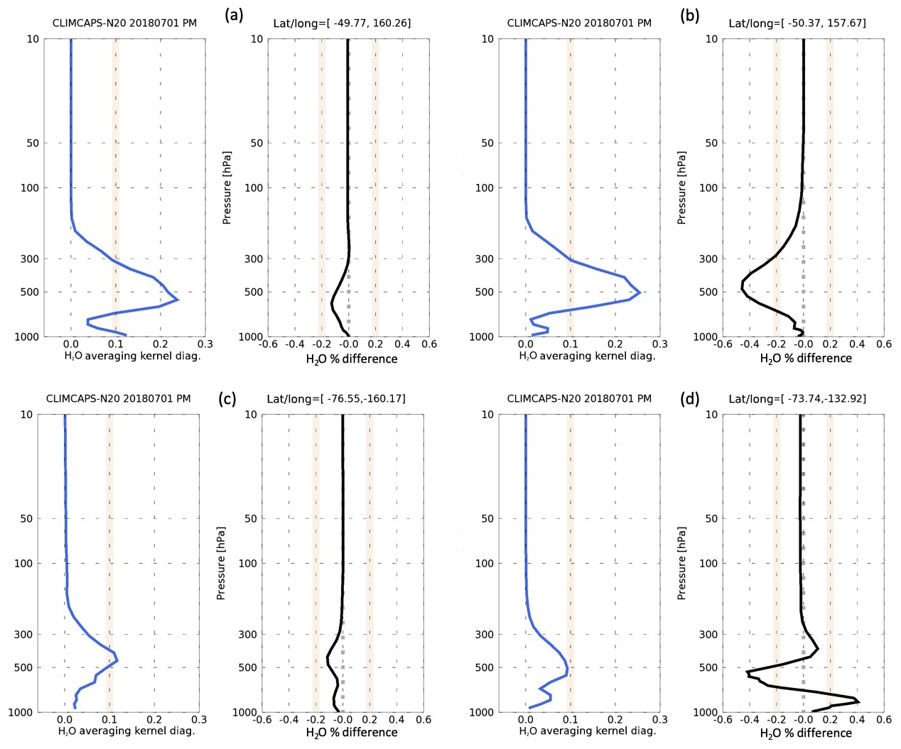
Figure 10 Towards a generalized diagnostic analysis of CLIMCAPS-NOAA20 retrievals on 1 July 2018. We can broadly identify four different scenarios for CLIMCAPS water vapor (H₂O) retrievals by pairing the averaging kernel matrix diagonal (AKD; blue line) and retrieval departure (black line) calculated as percent difference: (a priori minus retrieval) ∕ (a priori). AKD is a metric for observing capability. The CLIMCAPS H₂O a priori is MERRA2, so the retrieval departure signifies a disagreement with measured radiances at a target scene. CLIMCAPS scenario (a) has strong observing capability and a small retrieval departure. Scenario (b) has strong observing capability and large retrieval departure. Scenario (c) has low observing capability and small departure. Scenario (d) has low observing capability and large departure. We empirically define the threshold for observing capability as 0.1 and for percent difference (a priori departure) as 20 %.

Data validation studies typically compare remote observations against dedicated aircraft and/or in situ measurements to derive a statistical estimate of overall product accuracy (Nalli et al., 2018a, b). While validation studies are critically important to determine mission objectives, they typically do not provide information on the accuracy of individual soundings from day to day or scene to scene. In science and operational applications, researchers regularly query individual soundings in their study of atmospheric processes and want to know how well a remote sounding represents the true atmospheric state at a specific scene. Radiosondes are launched daily but from a sparse network of sites; they are thus insufficient in determining site-specific accuracy for the thousands of satellite soundings each day. In Fig. 10, we introduce the four scenarios that emerge when pairing two CLIMCAPS metrics – a priori departure and the magnitude of AKDs – to propose them as a means to help facilitate product interpretation and characterization in the absence of “truth” data. They can help distinguish those cases in which a CLIMCAPS retrieval either departed from or stuck to its a priori due to higher sensitivity to the true state (large AKDs). A data user can have confidence that such cases are good representations of the true state. Alternatively, those cases with small a priori departures and small AKDs (scenario 3) should be interpreted with caution because the measurements lack the means (information content) with which to confirm or improve upon the a priori towards a better representation of the true state. Lastly, those retrievals with large a priori departures and low AKDs (scenario 4) should be rejected as a misrepresentation of the true state because the retrieval is mostly likely dominated by noise, not signal. The a priori may itself be close to the truth, but we cannot confirm this due to the system's inability to observe conditions at that scene.

CLIMCAPS has a series of quality control thresholds at various retrieval steps to test T and H₂O retrievals but has no such tests for trace gas variables specifically. As a post-processing step within data applications, the quality control tests are assembled into a data filter that removes unsuccessful T and H₂O retrievals or those with high uncertainty. Currently, the same filters are applied to all retrieved variables, with no distinction made between different variables at a target scene. We propose a method with which to diagnose CLIMCAPS retrievals on a case-by-case basis, one retrieval variable at a time. Instead of applying a blanket data filter, we illustrate how four diagnostic scenarios (Fig. 10, Table 3) can help a data user to characterize retrieval quality along its vertical axis, from the boundary layer to the top of the atmosphere. In Figs. 11 and 12 we build on this to illustrate how these scenarios also apply to CLIMCAPS retrievals horizontally, i.e., spatially across a swath of observations.

Figures 11 and 12 each have four panels: (a) a priori departures at 500 hPa, calculated as percent difference between CLIMCAPS retrieval and its MERRA2 a priori; (b) CLIMCAPS H₂O AKDs at 500 hPa as a metric of information content; (c) cloud clearing uncertainty quantified as the “amplification factor” of instrument random noise (Chahine, 1977); and (d) cloud fraction retrievals for each CrIS footprint (or field of view). Figure 11 is a daytime scene (∼ 13:30 local overpass time) over the Caribbean Ocean, including parts of northern Columbia and Venezuela, while Fig. 12 is a nighttime scene (∼ 01:30 local overpass time) over the southeast continental United States. Note how CLIMCAPS retrieval departures do not appear to be spatially random but are instead clustered into distinct features. This means that CLIMCAPS adds new spectral information to its MERRA2 a priori under specific conditions, which we can diagnose to determine information content and quality. Comparing panel (a) with (c) and (d), we see that there is no direct correlation between retrieval departure (difference between retrieval and a priori) and the presence of or uncertainty due to clouds. This means that CLIMCAPS does have the ability to separate spectral information about H₂O from clouds and add this to its a priori where necessary. In Figs. 11 and 12 we highlight specific features for discussion – solid lines indicate retrievals that passed all quality control tests and are labeled “good”, while dashed lines indicate retrievals that failed at least one quality control test and are labeled “bad”.

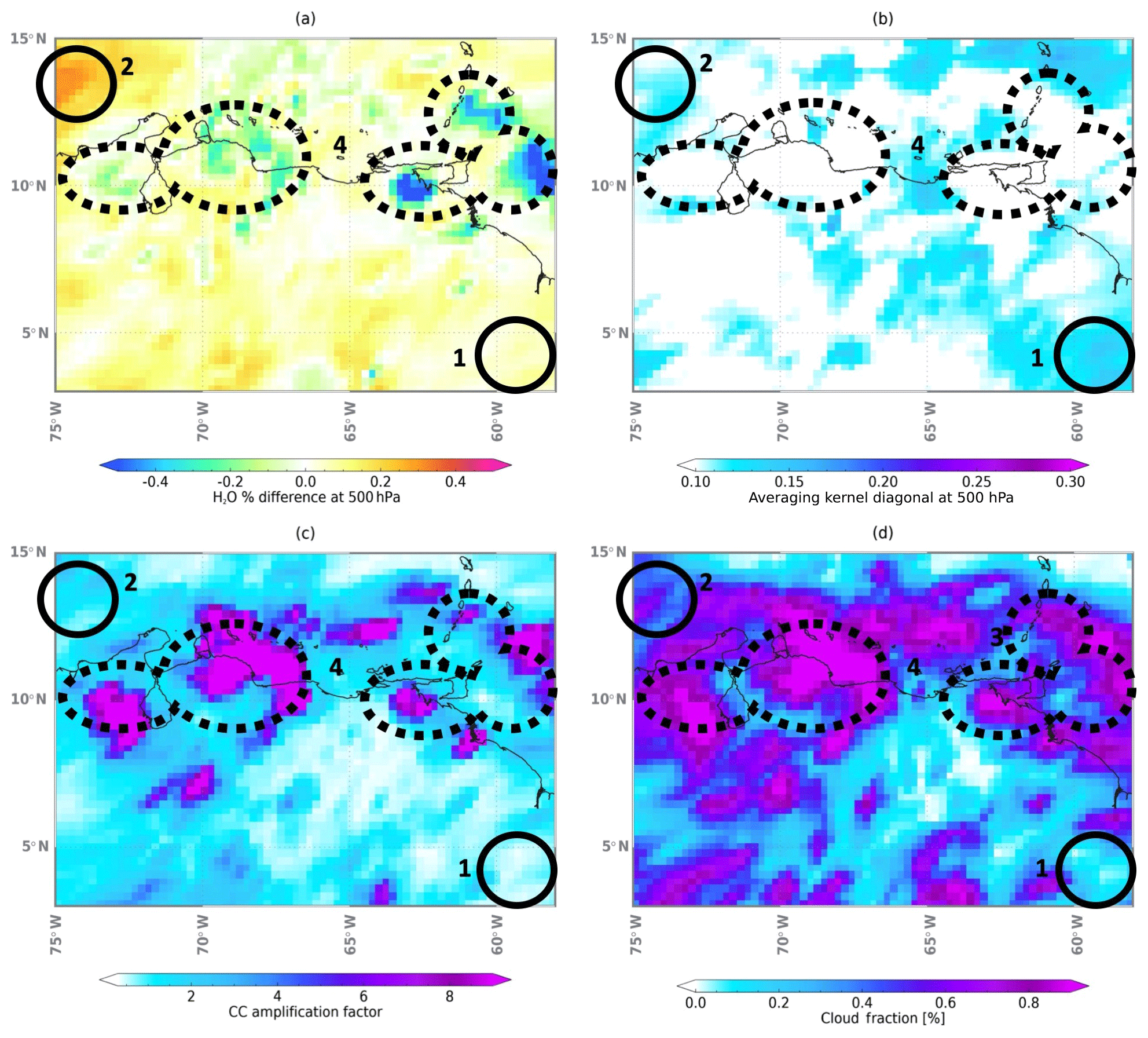
Figure 11 Diagnostic evaluation of CLIMCAPS-NOAA20 retrievals of H₂O for ascending Granule 89 (∼ 13:30 local overpass time) on 1 July 2018 over the Caribbean Sea as well as northern Colombia and Venezuela. (a) H₂O retrieval difference as percent departure from a priori, MERRA2, at 500 hPa. (b) Averaging kernel matrix diagonal vector at ∼500 hPa (AKD). (c) Cloud clearing (CC) amplification factor, a metric of uncertainty about clouds in the radiance signal. (d) Cloud fraction (%) retrieved for each CrIS field of view. Shapes with solid lines indicate scenes in which CLIMCAPS retrievals passed all quality control tests, and shapes with dashed lines indicate scenes in which CLIMCAPS retrievals failed at least one quality control test and are flagged as “bad”. We label each shape according to the scenario as depicted in Table 3. Shape 2 (scenario 2) has large a priori departure and large information content. Shape 4 (scenario 4) has large a priori departure and low information content. Shape 1 (scenario 1) has small a priori departure and high information content. Panels (c, d) provide additional diagnostic information about cloud cover and uncertainty.

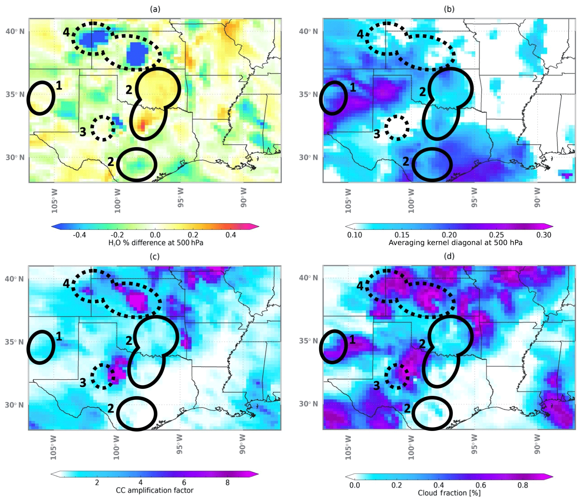
Figure 12 Same as Fig. 11 but for descending Granule 40 (∼ 01:30 local overpass time) on 1 July 2018 over the southern United States. (a) H₂O retrieval difference as percent departure from a priori, MERRA2, at 500 hPa. (b) Averaging kernel matrix diagonal vector at ∼500 hPa (AKD). (c) Cloud clearing (CC) amplification factor, a metric of uncertainty about clouds in the radiance signal. (d) Cloud fraction (%) retrieved for each CrIS field of view. We highlight features for which CLIMCAPS retrievals depart from MERRA2 (a priori) to demonstrate the diagnostic scenarios introduced in Fig. 10. Regions with solid lines indicate scenes in which CLIMCAPS retrievals passed all quality control tests, and regions with dashed lines indicate scenes in which CLIMCAPS retrievals failed at least one quality control test and are flagged as “bad”. We label each shape according to the scenario as depicted in Table 3. Shape 4 (scenario 4) has large a priori departure and low information content. Shape 3 (scenario 3) has small a priori departure and low information content. Shape 1 (scenario 1) has small a priori departure and high information content. Shape 2 (scenario 2) has large a priori departure and high information content. Panels (c, d) provide additional diagnostic information about cloud cover and uncertainty.

In Fig. 10 we use empirically defined thresholds to categorize retrievals into one of four scenarios: 0.1 for AKD and 0.2 for retrieval departure. Figures 11 and 12 demonstrate how they manifest spatially for specific features. Scenario 1, with a small a priori departure and high information content, is featured in (i) in Fig. 11 (shape 1), where the region has low cloud clover (<20 % cloud fraction) and very low cloud clearing uncertainty, as well as (ii) in Fig. 12 (shape 1) with varying cloud cover that exceeds 60 % at times but maintains a relatively low cloud clearing uncertainty. In both of these cases, retrievals passed CLIMCAPS quality control and maintained high information content and low cloud uncertainty, so they can be used in applications with confidence and be interpreted as a confirmation of the MERRA2 values for mid-tropospheric moisture. Scenario 2, with a large a priori departure and high information content, is featured in (i) in Fig. 11 (shape 2), where CLIMCAPS retrievals increase MERRA2 H₂O values at 500 hPa by as much as 30 % and despite significant cloud cover maintain low cloud uncertainty, as well as (ii) in Fig. 12 (shape 2, centered at 35^∘ N, 97.5^∘ W), where CLIMCAPS increases MERRA2 by 10 % over a large region and by as much as 40 % at a localized site at which cloud cover and uncertainty are both low. It is also featured in (iii) in Fig. 12 (shape 2 centered at 29^∘ N, 98^∘ W), where CLIMCAPS decreases MERRA2 mid-tropospheric moisture by 20 %. In these cases, retrievals passed quality control and maintained high information content in scenes with low cloud cover, so they can be used with confidence and interpreted as a legitimate departure from MERRA2 and a more accurate representation of the true state compared to MERRA2 alone. Scenario 3, with small a priori departure and low information content, is featured in (i) in Fig. 12 (shape 3), where information content is below the 0.1 threshold and retrieval departure below 20 %. These are retrievals that also failed CLIMCAPS quality tests (indicated by the dashed lines) but for reasons other than cloud uncertainty (which is low) and cloud cover (cloud clearing has high accuracy in partly cloudy scenes such as these). Scenario 4, with large a priori departure and low information content, is featured in (i) in Fig. 11 (shape 4) and (ii) in Fig. 12 (shape 4), where CLIMCAPS reduces MERRA2 H₂O values at 500 hPa by more than 50 % and information content is less than the 0.1 threshold. A very high cloud clearing uncertainty (>8 amplification of noise) and nearly solid cloud deck (>80 % cloud fraction) help explain why these retrievals failed quality control tests and should not be trusted in applications. Retrievals with information content less than 0.1 give us no information on the quality of MERRA2 values (we cannot confirm or deny that they correspond to top-of-atmosphere measured radiances and therefore know nothing about their accuracy); they only highlight that observing capability was low at that scene. We can diagnose this lack of observing capability, which in itself yields information about the atmospheric state such as cloud cover and uncertainty, but we cannot use the retrievals with any confidence in applications or scientific analyses. On any given global day, a significant majority of the CLIMCAPS retrievals fall into scenarios 1 and 2, which means that we can use them with confidence and interpret their departure from MERRA2 (or lack thereof) with confidence. Note that the spatial patterns depicted in panels (a) and (b) of Figs. 11 and 12 are unique to each retrieval variable and vary with pressure layers according to the AKD shape and vertical profile differences between the retrieval and a priori.

4 Summary and conclusion

In this paper we described our implementation of the Rodgers (2000) Bayesian OE inversion method for CLIMCAPS v2 with a specific focus on averaging kernels. We contrasted the Rodgers method for averaging kernels (Eq. 1) with our CLIMCAPS implementation (Eq. 2) and described the impact our approach has on retrieved products. CLIMCAPS is the NASA system for generating a continuous record of satellite soundings from two different instrument suites on multiple satellite platforms: AIRS/AMSU on Aqua and CrIS/ATMS on SNPP and NOAA20. CLIMCAPS products are publicly available through the NASA EOSDIS Earthdata portal, and each product file contains the full averaging kernel matrix (AKM) for seven retrieval variables at every scene – T, H₂O, CO, CH₄, CO₂, O₃, and HNO₃. CLIMCAPS AKMs vary in shape and magnitude across (i) retrieval variables according to top-of-atmosphere spectral sensitivity and instrument spectral resolution, (ii) satellite platforms according to instrument characteristics and retrieval algorithm assumptions, and (iii) retrieval scenes according to instrument effects such as view angle and environmental conditions like temperature lapse rates, uncertainty in interfering and background variables, and a priori assumptions about the target variable. At any given scene, the AKM for one variable is largely independent from that of another due to the CLIMCAPS sequential retrieval approach (Table 1; Smith and Barnet, 2019) and infrared channel selection to minimize spectral interference. For the first time, we compare the observing capability from CLIMCAPS-Aqua with CLIMCAPS-NOAA20 to diagnose and characterize continuity in information content across satellite platforms and instrument technology. In summary, we can state the following.

• The observing capability for T and H₂O is different between CLIMCAPS-Aqua and CLIMCAPS-NOAA20. This may be due to differences in how we regularize the OE solution for each satellite suite of instruments, but it may also reflect fundamental instrument differences; AIRS on Aqua is a grating spectrometer and CrIS on NOAA20 a Michelson interferometer. In the future, we will investigate this question.

• CLIMCAPS-NOAA20 has a higher observing capability for CO₂ in the mid-troposphere than CLIMCAPS-Aqua.

• CLIMCAPS has peak observing capability for CO and CH₄ in the mid-troposphere, with CO at ∼500 hPa and CH₄ at ∼300–400 hPa.

• CLIMCAPS information contents for T, H₂O, CO, and O₃ are largely independent of each other, with different spatial patterns in their derived DOF (trace of AKM).

• CLIMCAPS-NOAA20 has latitudinal variation in observing capability for H₂O, O₃, CO, CH₄, and CO₂. For H₂O, CLIMCAPS-NOAA20 observing capability peaks in the tropics (30^∘ S to 30^∘ N) at 300 hPa, while it peaks lower down at 450 hPa outside the tropics. CLIMCAPS-NOAA20 has the highest latitudinal variability for O₃, with the strongest peaks in the tropics in both the stratosphere and troposphere. CLIMCAPS-NOAA20 has almost no vertical stratification in observing capability in the polar regions (>60^∘ N and <60^∘ S). The midlatitude regions have O₃ AKM peaks in the stratosphere only. CO₂ AKMs have the strongest peak at 200 hPa in the tropics. Tropical CH₄ has much lower vertical resolution (as seen in its broad averaging kernel functions) with no distinct peak at 400 hPa as seen in other latitudinal zones.

• CLIMCAPS-Aqua has latitudinal variation in its observing capability for T, H₂O, O₃, CH₄, and HNO₃. It is lowest in the boundary layer for all variables. It has the highest vertical resolution (sharpest peak) for T at 700 hPa in the north polar region (>60^∘ N). CLIMCAPS-Aqua has lower observability for tropospheric O₃ in the tropics. HNO₃ AKMs have distinct latitudinal variation, with the highest observability in the stratosphere (<100 hPa) for all zones but the strongest in the north polar regions (>60^∘ N), followed by midlatitudes, south polar, and the tropics in that order.

• CLIMCAPS, whether from NOAA20 or Aqua, has sensitivity to O₃ and CO₂ in two broad layers, one in the mid-troposphere and another in the stratosphere (<50 hPa). It also has sensitivity to CO and CH₄ in one broad mid-tropospheric layer, HNO₃ in one broad stratospheric layer, and multiple narrow tropospheric layers for H₂O and T, with additional layers in the stratosphere for T.

We identified four scenarios with which to diagnose CLIMCAPS retrievals vertically along a pressure gradient on a scene-by-scene basis. These scenarios are (1) high observing capability (large AKD) and small a priori departure, (2) high observing capability (large AKD) with large a priori departure, (3) low observing capability (small AKD) with small a priori departure, and (4) low observing capability (small AKD) with large a priori departure. CLIMCAPS has additional uncertainty metrics for evaluating retrievals, such as cloud clearing amplification factor, radiance residual, cloud fraction and cloud-top height, DOF, retrieval covariance error, convergence strength, and whether a range of quality control thresholds were exceeded. As a long-term record of temperature, moisture, and trace gases that is continuous and consistent across instruments and satellite platforms, CLIMCAPS v2 products can be useful in characterizing diurnal and seasonal atmospheric processes from different time periods and regions across the globe.