A tropopause-related climatological a priori profile for IASI-SOFRID ozone retrievals: improvements and validation

The MetOp/Infrared Atmospheric Sounding Interferometer (IASI) instruments have provided data for operational meteorology and document atmospheric composition since 2007. IASI ozone (O₃) data have been used extensively to characterize the seasonal and interannual variabilities and the evolution of tropospheric O₃ at the global scale. SOftware for a Fast Retrieval of IASI Data (SOFRID) is a fast retrieval algorithm that provides IASI O₃ profiles for the whole IASI period. Until now, SOFRID O₃ retrievals (v1.5 and v1.6) were performed with a single a priori profile, which resulted in important biases and probably a too-low variability. For the first time, we have implemented a comprehensive dynamical a priori profile for spaceborne O₃ retrievals which takes the pixel location, time and tropopause height into account for SOFRID-O3 v3.5 retrievals. In the present study, we validate SOFRID-O3 v1.6 and v3.5 with electrochemical concentration cell (ECC) ozonesonde profiles from the global World Ozone and Ultraviolet Radiation Data Centre (WOUDC) database for the 2008–2017 period. Our validation is based on a thorough statistical analysis using Taylor diagrams. Furthermore, we compare our retrievals with ozonesonde profiles both smoothed by the IASI averaging kernels and raw. This methodology is essential to evaluate the inherent usefulness of the retrievals to assess O₃ variability and trends. The use of a dynamical a priori profile largely improves the retrievals concerning two main aspects: (i) it corrects high biases for low-tropospheric O₃ regions such as the Southern Hemisphere, and (ii) it increases the retrieved O₃ variability, leading to a better agreement with ozonesonde data. Concerning upper troposphere–lower stratosphere (UTLS) and stratospheric O₃, the improvements are less important and the biases are very similar for both versions. The SOFRID tropospheric ozone columns (TOCs) display no significant drifts (<2.5 %) for the Northern Hemisphere and significant negative ones (9.5 % for v1.6 and 4.3 % for v3.5) for the Southern Hemisphere. We have compared our validation results to those of the Fast Optimal Retrievals on Layers for IASI (FORLI) retrieval software from the literature for smoothed ozonesonde data only. This comparison highlights three main differences: (i) FORLI retrievals contain more theoretical information about tropospheric O₃ than SOFRID; (ii) root mean square differences (RMSDs) are smaller and correlation coefficients are higher for SOFRID than for FORLI; (iii) in the Northern Hemisphere, the 2010 jump detected in FORLI TOCs is not present in SOFRID.

1 Introduction

Ozone (O₃) in the stratosphere protects life from solar UV radiation. Close to the surface, O₃ is an oxidative pollutant harmful for human health through irritation of respiratory tracts (Brunekreef and Holgate, 2002) and for vegetation through deposition on leaves that leads to the reduction of plant growth (Ainsworth et al., 2012). Tropospheric O₃ is also a powerful greenhouse gas whose increase during the 20th century has significantly contributed to global warming (Shindell et al., 2006). The radiative forcing of O₃ is particularly important in the tropical upper troposphere–lower stratosphere (UTLS) (Chen et al., 2007).

It is therefore important to document the evolution of O₃ in these different layers independently. There is clear evidence from satellite databases that upper stratospheric O₃ has increased since 1997 following the ban of chlorofluorocarbons (CFCs) by the Montreal Protocol (Ball et al., 2018). Nevertheless, the total column O₃ has been stable since 1998. According to Ball et al. (2018), this contradiction is due to the fact that lower stratospheric O₃ is declining and compensates both stratospheric and tropospheric O₃ increase. Based on Ozone Monitoring Instrument/Microwave Limb Sounder (OMI/MLS) tropospheric ozone columns (TOCs), they state that TOC is globally increasing. OMI/MLS data for the 2005–2016 period are indeed documenting global positive TOC trends with particularly large increases over Asia (Ziemke et al., 2019). Based on 10 years of retrievals with the Fast Optimal Retrievals on Layers for Infrared Atmospheric Sounding Interferometer (IASI) O₃ (FORLI-O3) software, Wespes et al. (2018) document a decrease in tropospheric O₃ levels in the Northern Hemisphere (NH). Another IASI tropospheric O₃ product (Karlsruhe Optimized and Precise Radiative transfer Algorithm Fit; KOPRAFIT-O3) displays a TOC decrease over continental China (Dufour et al., 2018). In their exhaustive work on TOC evolution, Gaudel et al. (2018) clearly highlight the contradiction between global increase (OMI/MLS and other UV–vis products) on the one hand and global decrease (IASI) on the other hand. They also show that the different satellite products agree on a TOC increase over Asia. Among the two global IASI TOC datasets used in Gaudel et al. (2018), FORLI-O3 indicates a significant global decrease and O₃ retrievals with the SOftware for a Fast Retrieval of IASI Data (SOFRID) indicate a slightly weaker and less significant one. Two versions of FORLI-O3 have been validated by Boynard et al. (2016) (v20141022) and Boynard et al. (2018) (v20151001). They both document a jump in the O₃ retrievals in 2010 but this does not hinder the fact that TOCs are decreasing according to Wespes et al. (2017). It has to be noted that both validation studies compare IASI retrievals to ozonesonde profiles smoothed by the retrieval averaging kernels. Such a comparison enables the detection of abnormal biases, variability or drifts in the retrievals but does not document the ability of FORLI-O3 to reproduce real O₃ levels and variabilities. SOFRID-O3 has only been validated at the beginning of the IASI period on a very short time period (Barret et al., 2011) and on a longer time period together with FORLI-O3 and KOPRAFIT-O3 (Dufour et al., 2012). Furthermore, the European Organisation for the Exploitation of Meteorological Satellites (EUMETSAT) L2 atmospheric temperature products retrieved from IASI and used for FORLI (v20141022 and v20151001) and for SOFRID-O3 v1.5 retrievals are not stable in time (Boynard et al., 2018). Therefore, we have reprocessed the whole IASI database using ECMWF operational analyses for temperature and humidity to produce SOFRID-O3 v1.6. SOFRID-O3 has been shown to overestimate low tropospheric ozone over the Southern Hemisphere (SH) (Dufour et al., 2012; Emili et al., 2014, 2019). Emili et al. (2014) have hypothesized that this overestimation was due to the use of a single a priori profile biased towards NH midlatitudes O₃. In order to verify this hypothesis and to improve our O₃ retrievals, we have developed a new version of SOFRID-O3 (v3.5), with a dynamical a priori profile based on a global O₃ climatology (Sofieva et al., 2014).

The aim of the present paper is to validate both of the latest SOFRID-O3 products (v1.6 and v3.5) for the whole IASI period (2008–2017) in order to infer their ability to reproduce tropospheric O₃ levels and variability on seasonal to decadal timescales. The validation is based on O₃ profiles from ozonesondes retrieved from the World Ozone and Ultraviolet Radiation Data Centre (WOUDC) database. In Sect. 2, we describe the characteristics and differences of SOFRID-O3 v1.6 and v3.5 retrievals. Section 3 is dedicated to the description of the validation methodology based on comparisons between smoothed and raw ozonesonde data, and we provide our validation results in Sect. 4. Based on Boynard et al. (2018), we also compare our results to FORLI-O3 (Sect. 5) before concluding the paper in Sect. 6.

2 IASI SOFRID-O3 retrievals

IASI is a spaceborne thermal infrared nadir spectrometer. IASI has a moderate spectral resolution combined with a high signal-to-noise ratio and a 12 km footprint at nadir (Clerbaux et al., 2009). Thanks to its large across-track scanning (∼2200 km), IASI revisits each scene twice daily around 09:30 LT solar time in the morning and in the evening. Three IASI instruments have been launched on the MetOp meteorological platforms (MetOp-A in 2006, MetOp-B in 2012 and MetOp-C in 2018). Here, we present results based on O₃ retrievals from 10 years of MetOp-A/IASI data. We will present results based on the morning overpass data only as they are known to provide more information than nighttime data. Furthermore, it facilitates the comparison to other validation studies (Boynard et al., 2018) also based on morning data.

The SOFRID software first described in Barret et al. (2011) is based on the RTTOV (Radiative Transfer for TIROS Operational Vertical Sounder) operational radiative transfer code (Saunders et al., 1999; Matricardi et al., 2004) combined with the 1D-Var software (Pavelin et al., 2008), both developed within the framework of EUMETSAT Numerical Weather Prediction Satellite Applications Facility (NWP-SAF). The O₃ profiles are retrieved from the 980–1100 cm⁻¹ spectral window encompassing the 9.6 µm O₃ absorption band. Only cloud-free or weakly contaminated pixels are processed. Pixels with Advanced Very High Resolution Radiometer (AVHRR)-derived fractional cloud cover larger than 25 % are excluded. We also use a test based on brightness temperatures at 11 and 12 µm when AVHRR cloud cover is not available as described in Barret et al. (2011). The two SOFRID-O3 versions that are validated and compared in the present paper have significant differences that are described below.

2.1 Single a priori profile: v1.6

SOFRID-O3 v1.6 is almost similar to v1.5 described in Barret et al. (2011). It is based on RTTOV v9.3 (Saunders et al., 1999). In RTTOV, the optical depths are expressed as a linear combination of profile-dependent predictors that are functions of temperature, absorber amount, pressure and viewing angle. In RTTOV v9.3, the regression coefficients are derived from computations with the line-by-line radiative transfer model v11.6 (LBLRTM; Clough et al., 2005) on 43 atmospheric levels using the HITRAN2004 spectroscopic database (Rothman and Jacquemart, 2005). The single difference is that v1.6 uses temperature and humidity profiles from ECMWF operational analyses for the RTTOV simulations and v1.5 was using IASI L2 products delivered by EUMETSAT. The change has been operated for availability problems and mostly because the EUMETSAT L2 products are not homogeneous over the whole 2008–2017 period, which could result in retrieval inconsistencies (Boynard et al., 2018). We use 6-hourly ECMWF analyses which are provided on 91 (137) vertical levels until (after) 24 June 2013 from the ground up to 0.02 hPa on a $\mathrm{0.25}{}^{\circ }\times \mathrm{0.25}{}^{\circ }$ horizontal grid. The ECMWF temperature and humidity profiles are interpolated to the time and location of the target IASI pixel with a 3-D linear interpolation scheme.

O₃ concentrations are retrieved on the 43 RTTOV levels with the NWP-SAF 1D-Var algorithm (Pavelin et al., 2008) based on the optimal estimation method (OEM) (Rodgers, 2000). The OEM is a Bayesian method where the incomplete information provided by the measurement is complemented by a priori information which is supposed to represent the best knowledge of the state vector at the moment of the measurement. In our case, the state vector is the O₃ profile. For both v1.5 and v1.6, we use a single O₃ a priori profile which is based on 2 years (2008–2009) of WOUDC and Measurement of Ozone on Airbus In-Service Aircraft – In-Service Aircraft for a Global Observing System (MOZAIC-IAGOS) profiles completed to the top of the RTTOV v9.3 model (0.1 hPa) by MLS-averaged profiles (see Barret et al., 2011 for details).

2.2 Dynamical a priori profile: v3.5

As v1.6, SOFRID-O3 v3.5 uses interpolated temperature and humidity profiles from ECMWF analyses. It is based on the more recent RTTOV (v11.1) (Hocking et al., 2015), where regression coefficients are derived from LBLRTM v12.2 computations on 101 vertical levels with the HITRAN2008 spectroscopic database (Rothman et al., 2009). The second and more important one is that it uses dynamical a priori profiles from TpO₃, the O₃ profile tropopause-based climatology of Sofieva et al. (2014). This climatology is based on ozone profiles resulting from merging ozonesonde data in the troposphere and SAGE II v6.2 data (Wang et al., 2006) in the stratosphere. The ozonesonde profiles (36 000) extracted from the Binary Database of Profiles (BDBP) come from 136 stations for the period 1980 to 2006 (Hassler et al., 2008). For each merged ozonesonde–SAGE II profile, the tropopause was computed according to the World Meteorological Organization (WMO) definition of the lapse-rate tropopause (WMO, 1957). For each month, the ozone profiles are gathered according to 10^∘ latitude bins and 1 km tropopause intervals, and the corresponding averaged profiles together with their 1σ variabilities are computed and provided. Variable a priori profiles have already been used for satellite sensor retrievals. For instance, Tropospheric Emission Spectrometer (TES) O₃ retrievals used monthly mean profiles from the Model for OZone and Related chemical Tracers (MOZART) chemistry–transport model (CTM) averaged over a 10^∘ latitude $\times \mathrm{60}{}^{\circ }$ longitude grid (Bowman et al., 2006). OMI O₃ a priori profiles are based on a monthly and latitude-dependent ozone profile climatology (McPeters et al., 2007) derived from ozonesonde and satellite data (Liu et al., 2010). Nevertheless, the use of an a priori profile simply based on the geographical location of the satellite pixel does not allow taking the atmospheric dynamics into account. For instance, at a midlatitude location, the O₃ profile can be typical of midlatitudes on one day and polar (low tropopause) or tropical (high tropopause) a few days later depending on the global atmospheric dynamics (position of the polar or subtropical jets, anticyclones). The use of a tropopause-dependent climatology allows us to take the atmospheric dynamics into account and provides a more accurate a priori O₃ profile. This technique was once used for O₃ total column retrievals from Fourier-transform infrared spectroscopy (FTIR) spectra at the Jungfraujoch station (De Maziere et al., 1999). It was shown that the retrieved O₃ columns were largely improved when the tropopause was taken into account in the choice of the a priori profile. In a first attempt to take the tropopause into account for satellite retrievals, Sellitto et al. (2013) have implemented two a priori profiles in the KOPRAFIT-O3 retrieval algorithm to basically discriminate the tropics (tropopause higher than 14 km) from other latitudes. Dufour et al. (2015) have slightly improved the approach with a set of three a priori profiles for high latitudes (tropopause lower than 10 km), midlatitudes (tropopause between 10 and 14 km) and the tropics (tropopause higher than 14 km). Eremenko et al. (2019) have tested a set of profiles for retrievals on a synthetic database. In SOFRID-O3 v3.5, we compute the tropopause using the WMO lapse-rate definition from the ECMWF interpolated temperature profiles. The a priori profile is then picked up from the TpO₃ climatology according to month, latitude and tropopause height.

2.3 Information content and retrieval error

A remote sensing instrument is not equally sensitive to the different atmospheric layers. Its vertical sensitivity depends on its instrumental characteristics and on local parameters. In the case of a thermal infrared nadir sounder such as IASI, surface parameters such as surface emissivity, surface temperature, thermal contrast between the surface and the first atmospheric layer are key parameters to determine the vertical sensitivity, especially in the lower troposphere (Barret et al., 2005; Boynard et al., 2016). The vertical sensitivity of a remote sensing instrument is characterized by the so-called averaging kernel (AK) matrix. For each retrieval layer, the retrieved quantity is the result of the convolution of the whole real profile by the corresponding averaging kernel (row of the AK matrix) plus a contribution from the a priori profile (x_a) and a noise (ϵ) contribution (see Eq. 1).

$$\begin{array}{}\text{(1)}& \widehat{\mathit{x}}=\mathbf{A}\mathit{x}+(\mathbf{I}-\mathbf{A}){\mathit{x}}_{\mathrm{a}}+\mathbf{G}\left(\mathit{ϵ}\right)\end{array}$$

In an ideal case, the AK matrix (A) would be the identity matrix (I) and real (x) and retrieved ($\widehat{\mathit{x}}$) profiles would be identical within the noise level (ϵ) contribution. G is the gain matrix that represents the sensitivity of the retrieval to the measurement. In a real case, the AKs are bell-shaped functions which peak at an altitude that could be different from the nominal altitude and whose width gives an indication of the retrieval vertical resolution.

The degree of freedom for signal (DFS) of a retrieval describing the number of independent pieces of information provided by the measurement is the trace of the AK matrix (Rodgers, 2000). We have divided the atmosphere in five layers which are described in Table 1. The troposphere-2 layer has been selected for comparison with Boynard et al. (2018), who did not compute a tropopause-based TOC for their validation (see Sect. 5). The DFS corresponding to these different layers is displayed in Fig. 1 for v1.6 and v3.5 averaged over the validation dataset. The total DFS ranges from 2.4 to 3.3 for v3.5 and is about 0.2 lower for v1.6. The DFS values for the troposphere (WMO lapse rate), UTLS and stratosphere are almost identical for both versions. The tropospheric DFS is the lowest (0.3–0.5) at high latitudes where surface temperature, thermal contrast and tropopause height are the lowest and the highest in the tropics (about 1.5) where surface temperature and tropopause height are the highest. At midlatitudes, the tropospheric DFS is about 0.6. Therefore, except in the tropics, SOFRID retrievals provide less than one independent piece of information in the troposphere. In the UTLS (stratosphere), the DFS values range from 0.7 to 1 (from 0.9 to 1.5), which means that SOFRID provides around one independent piece of information in these layers.

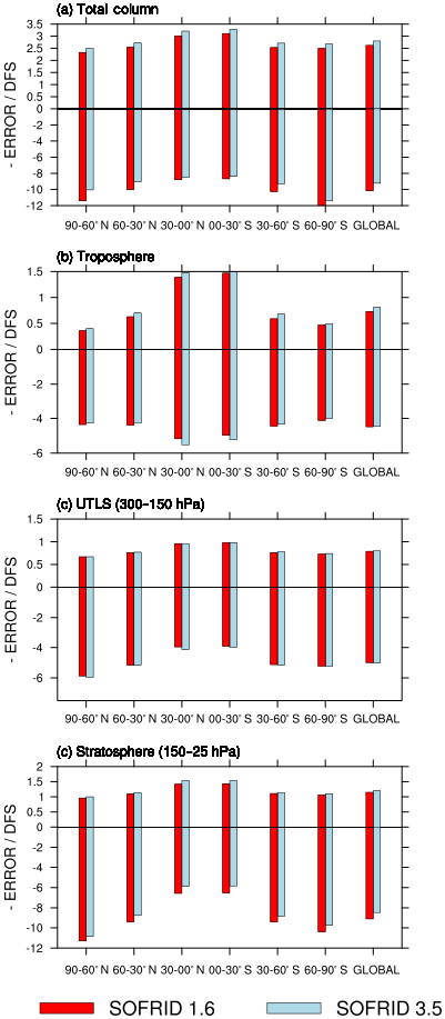
Figure 1 DFS and (–) retrieval errors in Dobson units (DU) for SOFRID-O3 v1.6 (red) and v3.5 (light blue) retrievals for (a) total column, (b) troposphere, (c) UTLS (300–150 hPa) and (d) stratosphere (150–25 hPa).

Table 1 Atmospheric layers for comparisons.

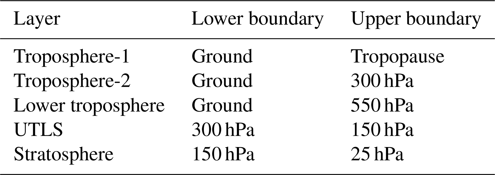
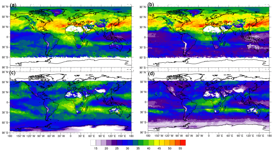
Figure 2 TOC distributions in DU for (a) July 2017 v1.6, (b) July 2017 v3.5, (c) December 2017 v1.6 and (d) December 2017 v3.5.

The retrieval error is the sum of the measurement and smoothing errors (Rodgers, 2000). Uncertainties in auxiliary parameters (temperature and humidity profiles, surface properties, etc.) are also responsible for errors. Coheur et al. (2005) and Barret et al. (2005) have shown that in the case of O₃ and CO retrievals from thermal infrared satellite sensors, the dominant source of errors was the smoothing error. The retrieval errors for SOFRID-O3 v1.6 and v3.5 are displayed in Fig. 1. Here, v1.6 displays slightly larger errors than v3.5 but has the same behavior. For the total and stratospheric columns, the errors decrease from high latitudes (9–12 DU) to the tropics (6–8 DU). The behavior of UTLS errors is similar with lower values (4 to 6 DU). For the TOC, errors are larger in the tropics (5 DU) than at middle and high latitudes (4 DU). This is due to the fact that the tropopause height is higher in the tropics, resulting in a larger a priori variability. The impact of the increased variability exceeds the one of the increased information content, resulting in a larger smoothing error.

2.4 Global distributions of tropospheric ozone columns

The global distributions of TOC from SOFRID v1.6 and v3.5 for July and December 2017 are displayed in Fig. 2. The global TOC structures are similar for both versions. They both clearly show the highest TOC over the NH midlatitudes in summer with a large export region over the northern Pacific off the Chinese coast and the summertime TOC maximum over the Eastern Mediterranean already documented with the Global Ozone Monitoring Experiment-2 (GOME-2) sensor (Richards et al., 2013). The tropical Wave-one pattern (Thompson et al., 2003; Sauvage et al., 2006) with the highest TOC over the tropical Atlantic and the lowest one over the South Pacific Convergence Zone (SPCZ) is also noticeable for both versions. Sauvage et al. (2006) have shown that the tropical Atlantic maximum was mostly a result of African and South American lightning NO_x (LiNOx) emissions. High TOCs are also detected during austral summer over southern Africa and the southern Indian Ocean towards Australia. According to Zhang et al. (2012), these high TOCs are mostly caused by LiNOx emissions from central Africa with a yearly maximum in May. The clearest difference between both versions is that v3.5 produces lower TOC than v1.6 in the low tropospheric O₃ regions. This is clear over the Intertropical Convergence Zone (ITCZ) and the SPCZ, over the SH for both seasons and over the NH midlatitudes in winter. We will show in the validation part of the paper that this is an important improvement of the SOFRID-O3 retrievals. The agreement is better in regions of high TOC such as NH midlatitudes in summer or the tropical Atlantic.

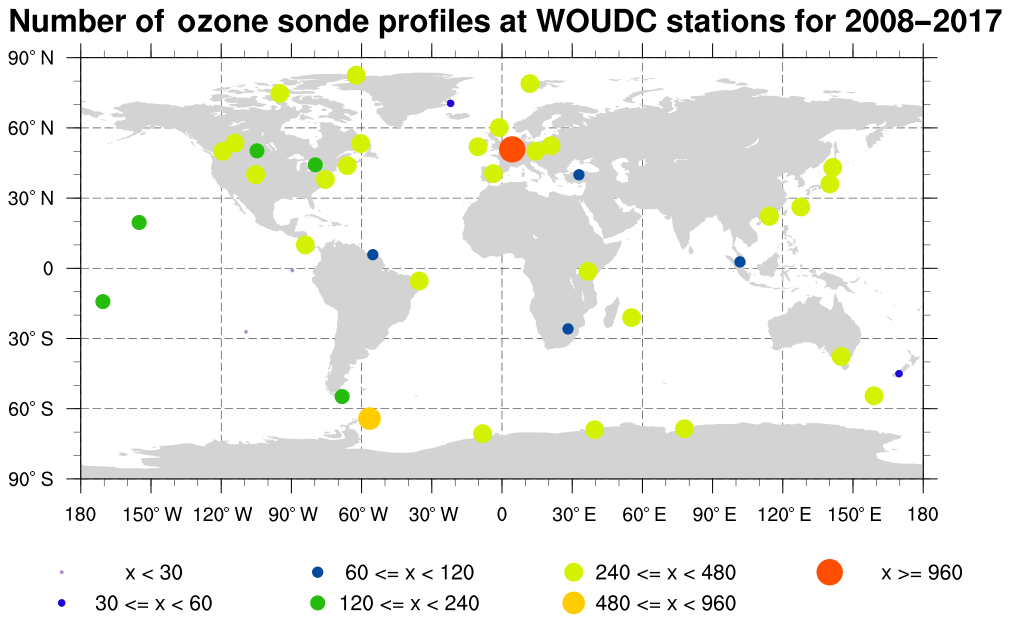
Figure 3 Maps of WOUDC stations with ECC O₃ sonde data during the 2008–2017 period. Colors and sizes of the markers indicate the number of valid sondes at each station.

The use of a dynamical a priori profile is responsible for visible stripes along the 10^∘ latitude bands. These stripes are generally indicating a discontinuity of 2.5 to 5 DU between two adjacent latitude bands with different a priori profiles. They are clearly caused by the impact of the a priori profile on the retrieval which is taken into account in the retrieval error (see Eq. 1). The latitudinal discontinuities are therefore consistent with our retrieval errors (4–5 DU) from Fig. 1. Such stripes may appear as a problem for the use of SOFRID v3.5 data for model validation. They are a minor problem for two main reasons. First, as is demonstrated in Sect. 4, the use of a dynamical a priori profile largely improves the retrieved O₃ profiles. Second, when model profiles are compared to SOFRID retrievals, the impact of the a priori profile is taken into account by using Eq. (1) such as in Barret et al. (2016).

3 Validation methodology

3.1 Ozonesonde data

Ozonesonde data come from the WOUDC database (https://www.woudc.org/, last access: 29 september 2020). For consistency purposes, we have chosen to use data from electrochemical concentration cell (ECC) sondes only. For the 10 years (the IASI period; 2008–2017), valid comparisons were effective for about 12 000 ozonesonde profiles among the 16 000 downloaded. A map with the number of sondes used for the validation at each station over the 2008–2017 period is displayed in Fig. 3. Most (∼7000) of the validation sondes were launched in the NH midlatitudes, with 15 stations providing more than one profile per month on average (more than 120 profiles for 10 years) mostly in western Europe and North America. For all other 30^∘ latitude bands, the number of validation profiles ranges from 800 to 1200, with only three to four stations providing more than 120 profiles. The balloons that carry the ozonesondes often explode below 40 km. In order to complete the ozonesonde profiles in the upper stratosphere and mesosphere, we have used MLS data averaged over 10 d on a $\mathrm{10}{}^{\circ }\times \mathrm{10}{}^{\circ }$ grid (see Barret et al., 2011 for details).

Figure 4 Taylor diagrams for (a, b) tropospheric columns and (c, d) lower tropospheric columns. (a, c) Raw sonde data, (b, d) smoothed sonde data. Red circles indicate v1.6; blue crosses indicate v3.5.

3.2 Coincidence criteria

The spatiotemporal coincidence criteria are ±1^∘ latitude, ±1^∘ longitude and ±12 h. They are similar to those used in Barret et al. (2011), Boynard et al. (2016) (50 km±10 h), Boynard et al. (2018) (100 km, ±6 h), Dufour et al. (2012) (110 km, ±7 h). As we compare sondes with IASI morning data only, and since most of the sonde launches are performed in the morning, using 6 or 12 h coincidence does not introduce significant differences. We have computed statistics for nine latitude bands which are the whole globe, the two hemispheres and six 30^∘ wide latitude bands. For each band, the monthly mean is computed if there are at least four coincident profiles within this latitude band. We first keep pixels for which convergence is achieved. Convergence is based on the value of the retrieval cost function output from the 1D-Var analysis (Jcost) which has to be positive, the value of its normalized gradient and the evolution of Jcost between the two last iterations (Havemann, 2020). We have also set an upper limit (1.0) for Jcost in order to eliminate pixels with poor-quality fits. Thirdly, only pixels with a total DFS>2.0 are selected. Using these criteria, we have kept about 9.0×10⁵ pixels out of 1.1×10⁶.

3.3 Comparison with raw and smoothed data

To compare remote-sensed to in situ or modeled profiles, it is important to apply Eq. (1) to the in situ or simulated profile (Rodgers, 2000; Barret et al., 2002). This procedure allows us to check the quality of the retrieval taking its degraded vertical resolution and sensitivity into account.

Nevertheless, in a validation objective, it is also necessary to compare the retrieved profiles to raw (not smoothed by the AKs) in situ profiles in order to perform a fully informative validation. This is of particular importance when the satellite data are used for issues such as the ozone seasonal to interannual variabilities (Wespes et al., 2017; Peiro et al., 2018) or to document the long-term tropospheric ozone tendencies (Gaudel et al., 2018; Wespes et al., 2018; Dufour et al., 2018). Indeed, the application of Eq. (1) implies the mixing of information between the different layers. Therefore, the variabilities and the drifts computed from raw and smoothed sonde data may be different and need to be documented. Raw ozone sonde data have been compared to IASI retrievals in few studies at the beginning of the IASI period (Barret et al., 2011; Dufour et al., 2012) but have been disregarded in more recent validation work (Boynard et al., 2016, 2018). The importance of raw data validation regarding seasonal and interannual variabilities and trends analyses will be highlighted in detail in Sect. 4.

3.4 Taylor diagram

In order to validate remote sensing with reference in situ observations, we need to determine how well they are able to reproduce the same behavior. There are four statistical indicators that have to be computed: (i) the absolute difference or bias which documents the accuracy, (ii) the root mean square of the differences (RMSDs) which tell whether the bias is significant or not, (iii) the coefficient of correlation (R) which documents the consistency and phase of the variabilities of both datasets and (iv) the ratio of the standard deviations of both datasets which documents the goodness of the amplitude of the retrieval variability. In the case of IASI O₃, the first three indicators are frequently computed (Boynard et al., 2016, 2018; Barret et al., 2011), but the last one is rarely compared (Dufour et al., 2012), which makes most validation exercises incomplete.

Based on the relationship between correlation coefficients, RMSDs and variances of the reference (validating) and test (validated) datasets, Taylor (2001) has developed the Taylor diagram initially for climate model evaluation. It displays all of these parameters (except the biases) in a more convenient and synthetic way than tables with numbers. Each experiment or observation to be validated correspond to a point placed within a quarter circle. The reference is located in the middle of the x axis (see Figs. 4, 5). The correlation coefficient between the reference and test dataset is given by the azimuthal position of the point. The RMSD is proportional to the distance between the test and the reference point. Finally, the radial distance from the origin is proportional to the variance of the experiment. We have normalized both RMSDs and standard deviations by the standard deviation of the reference to display the results from multiple experiments on a single diagram (see Taylor, 2001 for details).

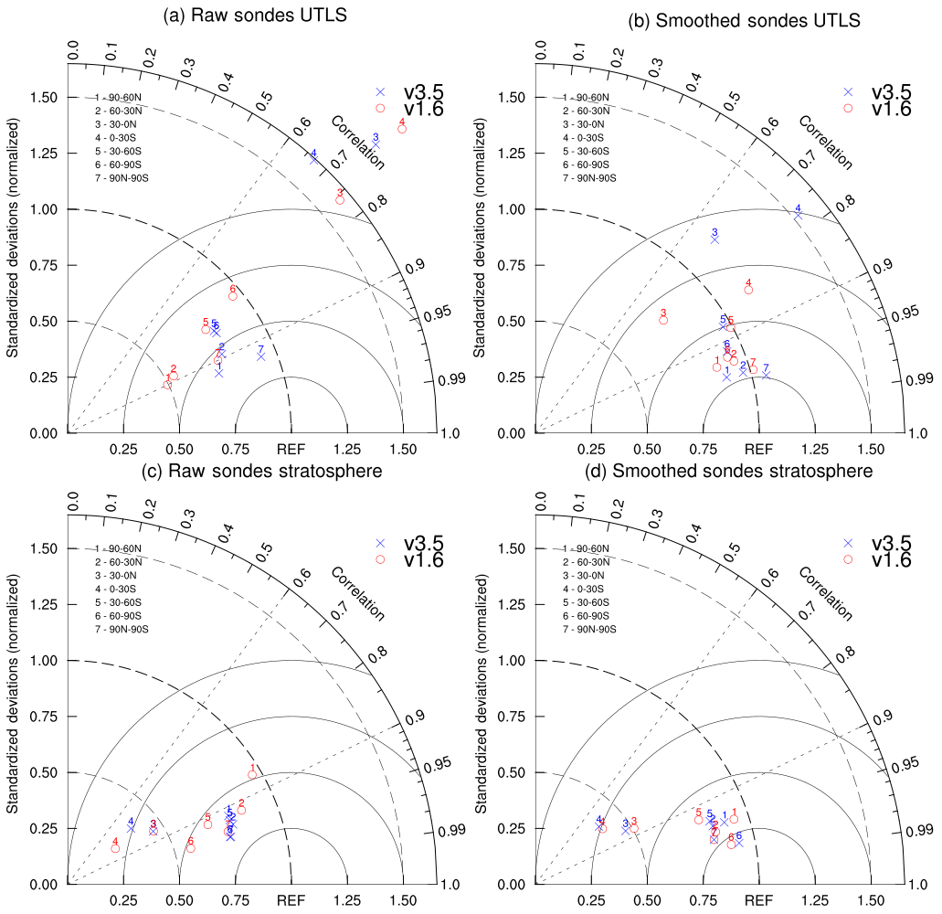
Figure 5 Taylor diagrams for (a, b) UTLS columns and (c, d) stratospheric columns. (a, c) Raw sonde data, (b, d) smoothed sonde data. Red circles indicate v1.6; blue crosses indicate v3.5.

4 Validation results

4.1 General statistics for tropospheric, UTLS and stratospheric partial columns

For the different latitude bands, the statistics from the comparisons between ozonesondes and SOFRID data are presented in Table 2 for the biases and corresponding RMSDs. Taylor diagrams are displayed in Fig. 4 for the TOC and lower tropospheric columns and in Fig. 5 for the UTLS and stratospheric columns.

Table 2 Biases (%) between sondes and SOFRID retrievals with corresponding RMSDs (%). Values between brackets correspond to smoothed sonde data. Significant biases (bias > RMSD) are in bold text.

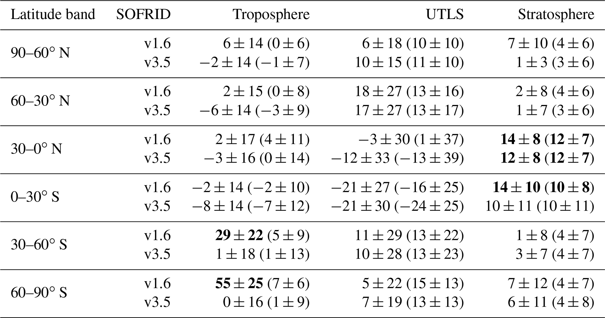
Concerning the troposphere, the comparison between SOFRID and raw sonde clearly shows the improvement from v1.6 to v3.5 (Fig. 4a). Here, v3.5 displays a larger variability in better agreement with the raw sonde data with a ratio between SOFRID and sonde variances ranging from 0.62 to 1.01. For v1.6, this ratio ranges from 0.15 to 0.45. The RMSDs of the SOFRID versus raw sonde data are lower and the correlation coefficients larger for v3.5 than for v1.6. Tropospheric biases are smaller than 10 % with the noticeable exception of midlatitudes and high latitudes of the SH for v1.6 and raw sonde data with significant biases of 29 % and 55 %, respectively (Table 2). This problem of SOFRID v1.6 retrievals in the SH had already been diagnosed by Dufour et al. (2012) and by Emili et al. (2014). The use of a dynamical a priori profile in v3.5 allows us to reduce these large biases to almost zero.

As expected, when the sonde profiles are smoothed with SOFRID AKs (Fig. 4b and d), the agreement between sonde data and SOFRID retrievals is better. The retrieval variabilities are closer to the sonde variabilities, the RMSDs are smaller, and the correlation coefficients are higher. It is also noticeable that differences between both retrieval versions are less important and that the improvement of v3.5 relative to v1.6 is less evident. Furthermore, the large v1.6 biases in the SH troposphere at midlatitudes and high latitudes are reduced below 10 % when the impact of the a priori profile is taken into account with Eq. (1), hiding the problem.

The lower tropospheric retrieved columns agree less with raw sonde data with degraded correlation coefficients and larger RMSDs (Fig. 4c) compared to the TOCs. For raw sonde data comparisons, the lower tropospheric variability is better for v3.5 than for v1.6. When the sondes are smoothed, the statistics are much better and similar to the TOC results (Fig. 4d). The added value of lower tropospheric columns relative to TOCs is therefore not obvious for SOFRID-O3.

In the UTLS, both v1.6 and v3.5 are in good agreement with raw sonde data (Fig. 5a) and the differences between both versions are much lower than for the tropospheric columns. Correlation coefficients range from 0.67 to 0.93, and the ratios between retrieved and raw sonde variances range from 0.5 to 1.0 at midlatitudes and high latitudes. For the northern and southern tropical latitudes, the correlations coefficients range from 0.6 to 0.75, and the variance ratios are between 1.6 and 2.1, highlighting a too-high variability retrieved in the tropical UTLS. In the UTLS, biases are positive (5 % to 18 %) at high latitudes and midlatitudes, and negative (−3 % to −21 %) at tropical latitudes and not significant because of large RMSDs.

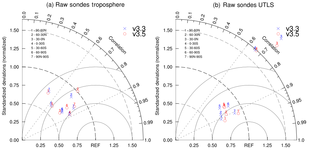
Figure 6 Taylor diagrams for (a) tropospheric columns and (b) UTLS columns for comparisons with raw sonde data. Red circles indicate v3.5; blue crosses indicate v3.3.

In the stratosphere, the agreement between raw sonde data and SOFRID retrievals is very good for the two versions as well as in all latitude bands, with correlation coefficients in the 0.75–0.98 range and variance ratios in the 0.56–0.96 range, except in the tropical bands where the retrieved variances are much lower than the ozonesonde variances (Fig. 4c). Stratospheric columns from v3.5 are in slightly better agreement (higher R², lower RMSDs) with ozonesonde data than v1.6. Large positive biases (10 %–14 %) are found at tropical latitudes for both v1.6 and v3.5 (Table 2).

Both in the UTLS and the stratosphere, the agreement is only slightly improved (larger correlation coefficients and lower RMSDs) when the sonde profiles are smoothed by the AKs (Fig. 5b and d). Smoothing of the sonde profiles does not significantly modify the UTLS and stratospheric biases. In particular, the tropical UTLS large negative biases are still present when the AKs are applied to the sonde data. The small differences between v1.6 and v3.5 on the one hand and between raw and smoothed sonde data on the other hand highlight the larger sensitivity of IASI to the UTLS and the stratosphere than to the troposphere as already discussed in Barret et al. (2011) and Dufour et al. (2012) for SOFRID v1.5.

4.2 Impact of the intraseasonal tropopause dependence of the a priori profile on SOFRID improvements

The Sofieva et al. (2014) climatology is tropopause dependent in two different ways. First, it implicitly documents the seasonal and latitudinal relationship between the tropopause and the O₃ profiles with the classification of the O₃ profiles by month and 10^∘ latitude band. Second, it explicitly documents the intraseasonal tropopause O₃ profiles' relationship with various tropopause-dependent profiles for each month and latitude band. In order to determine the impact of the intraseasonal tropopause dependence on the SOFRID retrievals, we have performed retrievals using the profile with the highest occurrence for each month and each 10^∘ latitude band as a priori information. The version with a single monthly a priori profile in each 10^∘ latitude band is v3.3.

The comparisons between v3.5 and v3.3 are presented in Taylor diagrams for the tropospheric and the UTLS columns in Fig. 6. In the stratosphere, the changes (not shown) are negligible. Concerning the TOC, the improvements are negligible except in the 60–30^∘ N and 60–90^∘ S bands where v3.5 better reproduces the variability of the TOC. In the UTLS, v3.5 gives slightly better results in terms of correlation coefficients and variability relative to v3.3 in all the latitude bands except in the 60–90^∘ S one. Nevertheless, the improvement from v3.3 to v3.5 is minor compared to the overall improvement from v1.6 to v3.5 (Figs. 4 and 5). We can therefore conclude that the seasonal (monthly) and latitude dependence of the a priori O₃ profile is responsible for most of SOFRID improvements.

4.3 Vertical profiles

After comparing partial columns, it is interesting to look at complete profiles to get better insight about the discrepancies between IASI retrievals and sonde data. The annual average profiles for v1.6 and v3.5 are displayed in Figs. 7 and 8, respectively, for the different latitude bands.

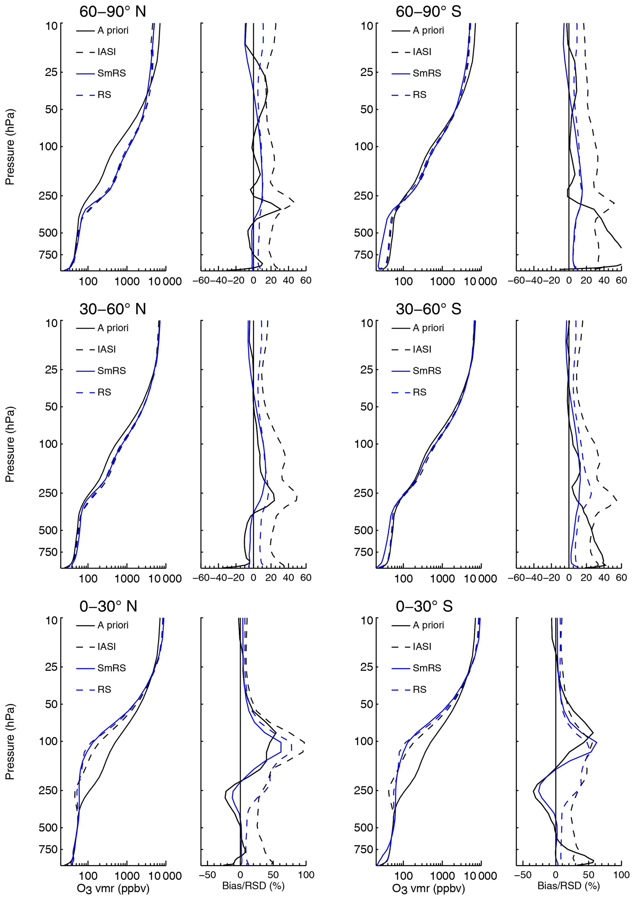
Figure 7 Profile comparisons between sonde and SOFRID-O3 v1.6 a priori profiles (left panels) (solid black lines), IASI (dashed black lines), smoothed (SmRS, solid blue lines) and raw (RS, dashed blue lines) sonde vertical profiles, biases (right panels) (solid lines) and RMSD (dashed lines) between IASI and raw (black lines) and smoothed (blue lines) sondes for the NH (left panels) and SH (right panels).

Figure 8 Same as Fig. 7 for SOFRID-O3 v3.5.

In the NH, v1.6 and v3.5 show similar behavior with a large upper tropospheric positive bias at midlatitudes and high latitudes and a large oscillation from a negative bias at 250 hPa to a large positive bias at 100 hPa in the tropics. These profile features are responsible for the positive (negative) biases for the midlatitudes and high latitudes (tropics) UTLS columns and for the positive biases for the tropical stratospheric columns (see Table 2). In the SH, the large tropospheric positive biases of SOFRID relative to raw sondes (below 300 hPa in the high latitudes and midlatitudes and below 500 hPa in the tropics) present in v1.6 almost disappear in v3.5. The improvement of SOFRID accuracy in the SH extratropical troposphere is the clearest advantage of using dynamical a priori profiles. In the SH tropics, the TOC difference between v1.6 and v3.5 is not so clear (see Table 2) because the positive bias in the lower troposphere is compensated by a larger negative bias in the upper troposphere in v1.6. As already discussed from column comparisons, it is also noticeable from profile comparisons (Figs. 7 and 8) that the agreement between SOFRID retrievals and smoothed sonde profiles is better than with raw sondes. An important exception are the large UTLS oscillations in both the NH and SH tropics and for both v1.6 and v3.5. Therefore, unlike what was expected, this important discrepancy between retrievals and sonde data does not result from the use of a single a priori profile too far from the real profile. The differences between v3.5 and v1.6 are largely reduced when sondes are smoothed. For instance, the large tropospheric biases for v1.6 in the SH disappear when the smoothing is applied to the sonde profiles.

For all latitude bands, RMSD profiles display the largest values around the tropopause (below 60 % in the extratropics and up to 100 % in the NH tropics), as is expected because it is the altitude range with the largest relative variability. RMSDs between retrievals and smoothed data are generally much lower than with raw data. This is also expected since the smoothing error is the largest source of error in IASI retrievals (see Barret et al., 2011; Dufour et al., 2012). RMSDs with smoothed sondes in the troposphere are somewhat larger for v3.5 than v1.6 especially in the SH. This is an indication of the increased sensitivity and decreased smoothing of v3.5. This is also evident in the Taylor diagrams which show that tropospheric variabilities are larger and in better agreement with sonde data (raw and smoothed) for v3.5 (see Fig. 4).

4.4 Time series of tropospheric columns

As tropospheric O₃ trend assessment is a major issue and one of the main topic of the TOAR (Tropospheric Ozone Assessment Report)/International Global Atmospheric Chemistry (IGAC) international initiative (Gaudel et al., 2018), we focus in this section on TOC time series. Time series are also interesting to bring insight about the general statistics discussed in the previous sections and to identify possible drifts of the data.

The time series of IASI and sonde monthly TOCs are presented in Fig. 9 (10) for v1.6 and in Fig. 11 (12) for v3.5 for the Northern (Southern) Hemisphere. We present both raw and smoothed sonde data to highlight the impact of smoothing upon the agreement between IASI and sondes. This impact is particularly obvious for SOFRID v1.6 at midlatitudes. At northern midlatitudes, the bias between SOFRID v1.6 and raw sonde TOCs displays large seasonal variations from −5 % to −10 % in summer and 10 % to 20 % in winter, resulting in a negligible 2 %±15 % average bias (Table 2). When sonde data are smoothed by IASI AKs, the sonde variability is largely reduced. Bias varies from 5 % in winter to −5 % in summer.

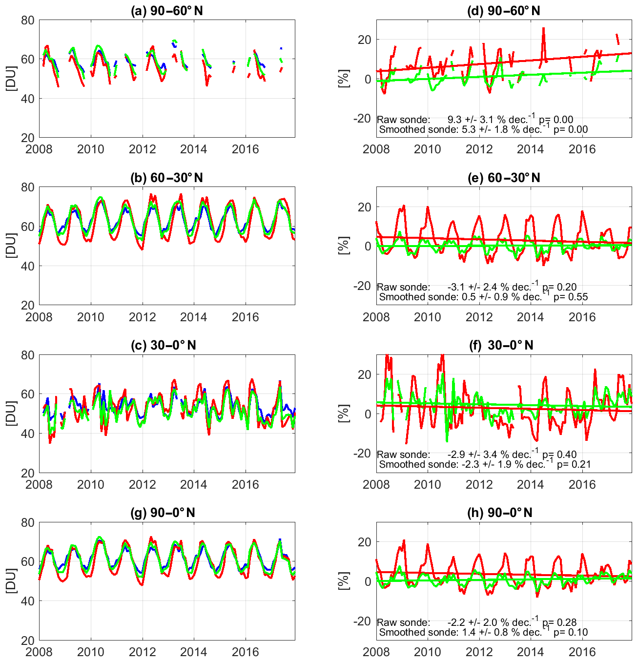
Figure 9 Time series of SOFRID-O3 v1.6 TOCs (DU) in the Northern Hemisphere for (a) 90–60^∘ N, (b) 60–30^∘ N, (c) 30–0^∘ N and (d) 90–0^∘ N. Blue lines indicate IASI retrievals, red lines indicate raw sonde data, and green lines indicate smoothed sonde data. Differences (%) between IASI and sonde data for (e) 90–60^∘ N, (f) 60–30^∘ N, (g) 30–0^∘ N and (h) 90–0^∘ N. Red lines indicate differences with raw sonde data and green lines indicate differences with smoothed sonde data.

Figure 10 Same as Fig. 9 for SOFRID-O3 v1.6 in the Southern Hemisphere.

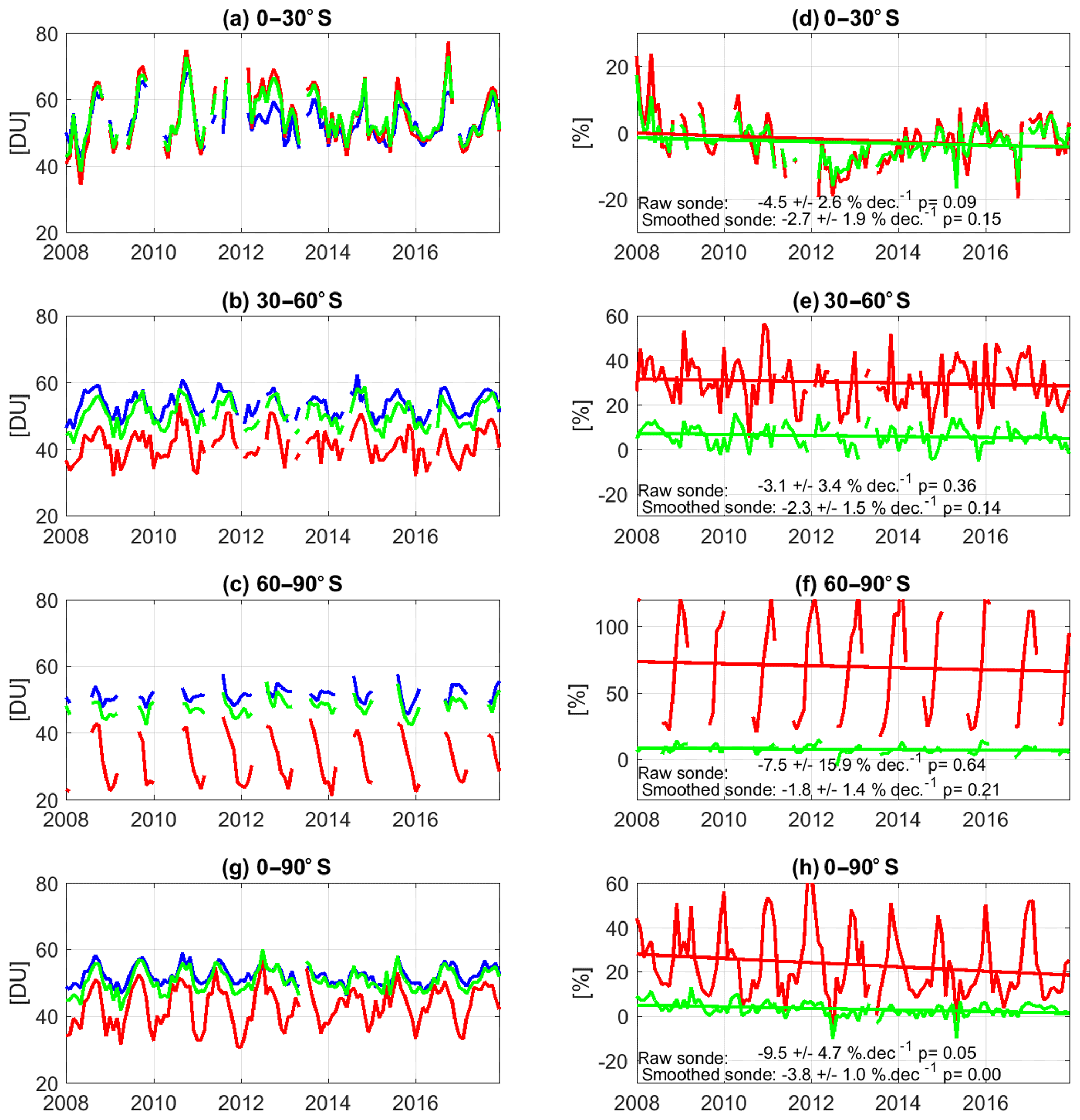
For southern midlatitudes, as already highlighted by Dufour et al. (2012) and Emili et al. (2014), SOFRID TOCs are significantly biased high (29 %±22 %) relative to raw sonde data (Table 2). This was explained by the fact that the single a priori profile used in v1.6 is biased towards northern midlatitude O₃ (Emili et al., 2014). When the sonde data are smoothed by IASI AKs, the agreement is much better and the bias becomes non-significant (5 %±9 %) as a result of taking the a priori contribution into account (Eq. 1). The largest significant bias (56 %±25 %) is found in the SH high latitudes for v1.6 TOCs (Table 2) with large seasonal variations from 20 % in winter to 120 % in summer. The large bias variabilities at midlatitudes and especially high latitudes of the SH result from the very low seasonal variability of the retrieved columns (see Fig. 4a).

Figure 11 Same as Fig. 9 for SOFRID-O3 v3.5 in the Northern Hemisphere.

Figure 12 Same as Fig. 9 for SOFRID-O3 v3.5 in the Southern Hemisphere.

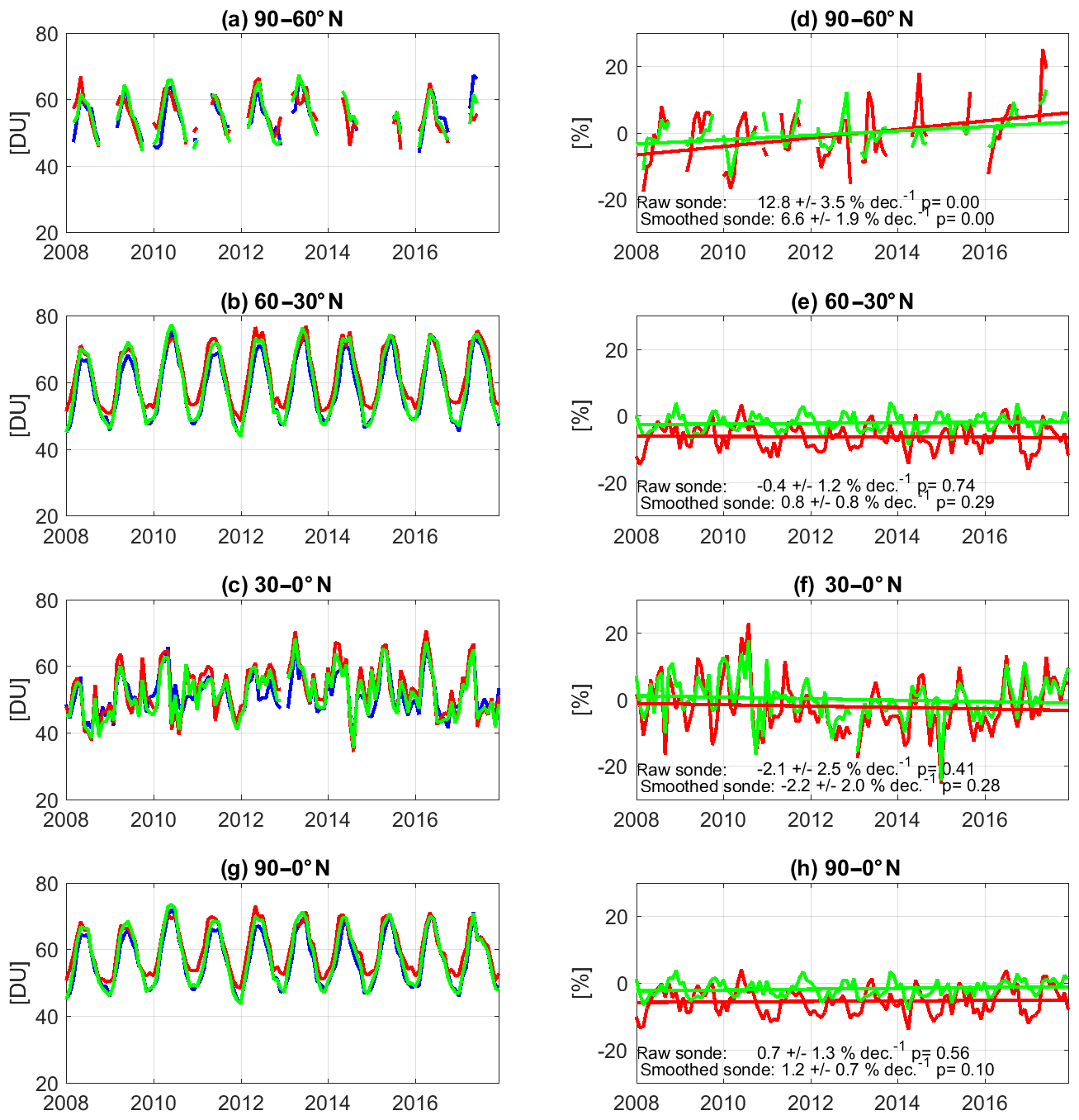
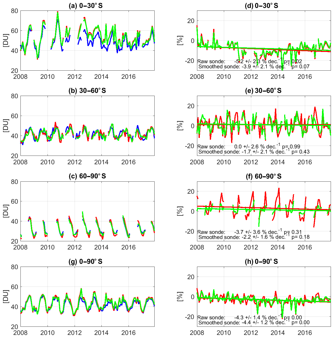
For v3.5, the use of a dynamical a priori profile clearly improves the retrievals at midlatitudes. At northern midlatitudes, the seasonal bias variation is reduced to −10 %–0 % and the average bias remains small ($-\mathrm{6}\mathit{\%}\pm \mathrm{14}$ %). When smoothing is applied, the seasonal variability almost disappears and the bias is only $-\mathrm{3}\mathit{\%}\pm \mathrm{9}$ %. At southern midlatitudes, the agreement is very good and very similar for raw and smoothed sonde data, with no real seasonal signature detectable and an average bias close to 0 %.

At tropical latitudes, the situation is quite different. First, the seasonal variability is not so notable and regular, and the difference between raw and smoothed sondes is lower than at midlatitudes. Furthermore, the behavior of v1.6 and v3.5 is close even though v3.5 is in better agreement with sonde data (see Sect. 4.1). In the southern tropics, there is a noticeable variation of bias between 2011 and 2014, with large negative biases of −10 % and −15 % for 2008–2010 and 2015–2017 with biases of 0 and −5 % for v1.6 and v3.5, respectively. As such a bias variation is not detected for other latitude bands, we assume that it may be linked to a gap in sonde data for the 2011–2014 period. A closer look at SH tropics' ECC sonde data shows that only two stations (Réunion and Nairobi) provide data regularly (30–50 profiles per year) over the period. For the Pago Pago Pacific station, data are available only from 2014 to 2016 and starting from 2012 for Irene in South Africa. For the Natal Atlantic station, more than 25 profiles are available during the 2008–2010 and 2014–2017 periods and almost none during the 2011–2013 period.

One issue that was raised in TOAR (Gaudel et al., 2018) was the different trends computed from different satellite products. UV–visible satellite sensors produce positive tropospheric O₃ burden trends in both hemispheres, while trends from IASI products are negative. It has to be noted that in Gaudel et al. (2018), negative O₃ burden trends from SOFRID v1.5 in the Northern Hemisphere and Southern Hemisphere, and for the whole Earth are, respectively, one-fourth, one-half and one-third smaller than FORLI's. The drifts computed from the SOFRID–sonde differences are displayed in Figs. 9 to 12.

At high northern latitudes, for both v1.6 and v3.5, the drifts are large (>9 % decade⁻¹ and >5 % decade⁻¹ for raw and smoothed data, respectively) and significant at the 95 % level. For midlatitudes and tropical latitudes, drifts are between 0.9 % decade⁻¹ and −3.4 % decade⁻¹ but are not significant. The NH midlatitude drift with raw sonde data is reduced from −3.1 with v1.6 to −0.4 % decade⁻¹ with v3.5. For the whole NH, the drifts are not significant and decreases from −2.2 with v1.6 to 0.7 % decade⁻¹ with v3.5 for raw sonde data. They are $<\mathrm{1.5}\mathit{\%}{\mathrm{decade}}^{-\mathrm{1}}\pm \mathrm{0.8}$ % decade⁻¹ and hardly significant (p>0.10) for smoothed sonde data.

In the SH tropics, drifts are $\sim -\mathrm{5}$ % decade⁻¹ and $\sim -\mathrm{3}$ % decade⁻¹ for raw and smoothed sonde data, respectively, and only significant for v3.5 compared to raw data. These drifts are linked to the large negative biases of the 2011–2014 period resulting from missing data (see above). For v1.6, a large but non-significant drift (−8 %) also occurs at high latitudes, which is largely reduced for v3.5. For the whole SH, we found a significant negative drift (relative to raw sonde data) of −9.5 % decade⁻¹ ± 4.7 % decade⁻¹ for v1.6 which is reduced to −4.3 % decade⁻¹ ± 1.4 % decade⁻¹ and becomes non-significant for v3.5.

5 Comparison with IASI-FORLI

Two versions of IASI O₃ retrievals with the FORLI software have been validated by Boynard et al. (2016) and Boynard et al. (2018) (B18). Part of their validation results are based on the same data as the present study, namely ECC ozone sondes from the WOUDC database between 2008 and 2014 for Boynard et al. (2016) and 2008 and 2016 for B18. As they document the latest FORLI version (v20151001) on a longer time period, we will focus on our comparison with B18. They have used a comparable number (11 600) of ozone sonde profiles as in the present study, and their comparison methodology is close to the one we have used (spatiotemporal coincidence criteria set to 100 km and ±6 h). We have collected the coefficients of determination (R²), the biases, the RMSDs, the DFS of the retrievals and the slopes of the linear fit between the smoothed sondes and retrievals from B18.

There are some limitations to the comparison between the validation of our SOFRID retrievals and the FORLI validation from B18. We are comparing our data with literature results which do not provide the same information as we do. For instance, B18 do not document the sonde and IASI variabilities, and it is therefore not possible to draw their data in Taylor diagrams. B18 have also limited their comparisons to smoothed sonde data. Another limitation is that FORLI and SOFRID use their own quality flags to filter the data. In order to document the impact of the pixel selection on SOFRID validation, we have performed the comparison with sonde data using modified quality flags. The cloud filtering threshold is the clearest source of difference between the pixel selection of both algorithms. We have therefore lowered the upper limit of the AVHRR cloud fraction cover to 13 %, which is the threshold used by B18, resulting in a loss of 5 % of the treated pixels. The Jcost threshold has been decreased from 1.0 to 0.15 with a 6 % decrease of the selected retrieved profiles. Finally, the DFS lower value has been set to 1.75, increasing the number of selected retrievals by 2 %. These threshold modifications resulted in negligible changes of the general statistics (bias, RMSD, R) for the three atmospheric layers (troposphere, UTLS and stratosphere) and the different latitude bands that are presented in this section. These statistics, based on large amounts of data, are therefore not hindered by pixel selection differences.

In Fig. 13, we have drawn DFS from SOFRID v1.6 and v3.5 and from FORLI for the layers selected by B18 (1013–300, 300–150 and 150–25 hPa). Figure 14 displays the coefficients of determination (R²) and the slopes (b) from linear relationships fitted between IASI retrievals and smoothed sonde data. Biases and RMSDs are shown for the three retrievals in Fig. 15. Finally, Fig. 16 documents the drifts between sondes and SOFRID retrievals for the whole NH for the surface–300 hPa layer to be comparable to B18.

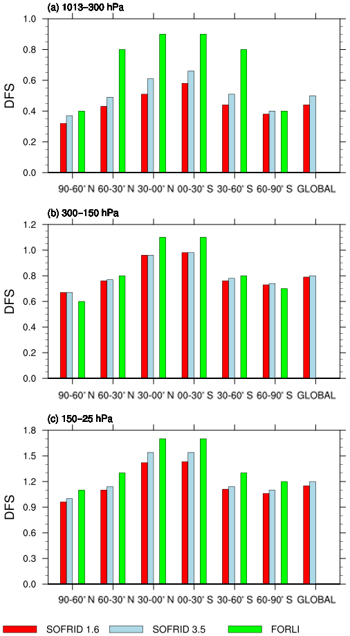
Figure 13 DFS of IASI SOFRID-O3 v1.6 (red), SOFRID-O3 v3.5 (light blue) and FORLI-O3 (green) retrievals in the different latitude bands for (a) 1013–300 hPa, (b) 300–150 hPa and (c) 150–25 hPa. FORLI data are taken from Boynard et al. (2018).

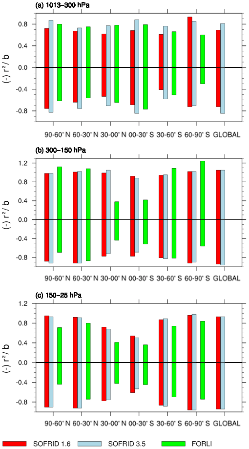
Figure 14 b indicates slopes of the linear regression (positive values), and (–) R² indicates coefficients of determination (negative values) between IASI retrievals and sonde data. Red indicates SOFRID-O3 v1.6, light blue indicates SOFRID-O3 v3.5, and green indicates FORLI-O3 (from Boynard et al., 2018).

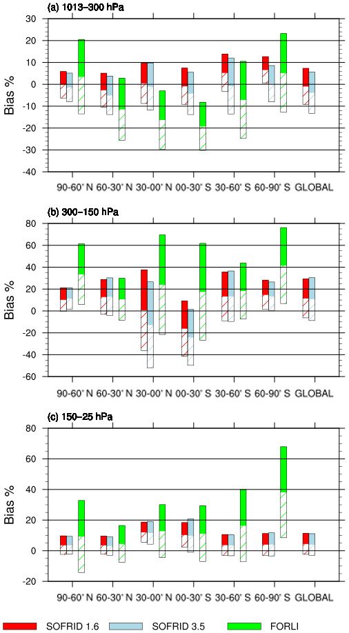
Figure 15 Biases and ±RMSDs (bars) of the differences between IASI retrievals and sonde data. Red indicates SOFRID-O3 v1.6, light blue indicates SOFRID-O3 v3.5, and green indicates FORLI-O3 (from Boynard et al., 2018).

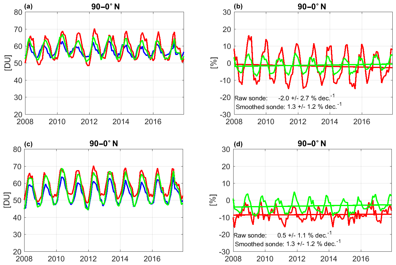
Figure 16 Time series of SOFRID-O3 (a) v1.6 and (c) v3.5 surface–300 hPa columns for the Northern Hemisphere (0–90^∘ N). Blue lines indicate IASI retrievals, red lines indicate raw sonde data, and green lines indicate smoothed sonde data. Differences between IASI and sonde data for (b) v1.6 and (d) v3.5. Red lines indicate raw sonde data and green lines indicate smoothed sonde data.

In the three atmospheric layers, the information content is larger with FORLI than with SOFRID v1.6 and v3.5 (Fig. 13). This is particularly visible for the midlatitudes and tropics in the troposphere with DFS of 0.8 to 0.9 for FORLI and DFS of only 0.4 to 0.6 for SOFRID. This probably results from the retrieval noise level which is lower for FORLI than for SOFRID (Dufour et al., 2012). At high latitudes, the DFS values are low and closer for both algorithms, and the increase from high to midlatitudes is therefore much larger for FORLI than for SOFRID. As both algorithms use a single retrieval noise and a priori covariance matrix and similar surface and atmospheric temperatures, the reason for such a difference is unclear. In the UTLS and stratosphere, the same increases of DFS from high latitudes to the tropics are visible for the three products. The difference in information content between retrievals is less pronounced in the UTLS and in the stratosphere than in the troposphere.

The RMSDs (see Fig. 15) are generally larger for FORLI than for SOFRID. In the troposphere, RMSDs reach 18 % for FORLI and are below 10 % for both SOFRID v1.6 and v3.5. In the UTLS, RMSDs are larger than in the other layers due to the lower absolute columns. For SOFRID, UTLS RMSDs are in the range of 10 %–30 % and 20 %–45 % for FORLI. For both SOFRID and FORLI, the highest RMSDs are in the tropics where the 150–300 hPa columns are the lowest. In the stratosphere, FORLI's RMSDs are also systematically larger than SOFRID's. The differences are the largest at high latitudes with FORLI RMSDs 3 to 4 times larger than SOFRID's.

The R² differences (Fig. 14) are partly related to the RMSD differences. Generally, SOFRID has larger R² than FORLI. As for the RMSDs, the differences between both algorithms are the largest at high latitudes (especially in the Southern Hemisphere where R²<0.4 for FORLI products) in the three layers. In the troposphere, the coefficients of determination are comparable for both algorithms in the tropical bands, and SOFRID v3.5 gives higher R² than SOFRID v1.6. The differences between retrieval versions are generally lower and can even be reversed in the UTLS and in the stratosphere.

The slopes of the linear fits between retrievals and sonde data provide complementary information to the R² coefficients. A slope smaller than 1 indicates that the retrieved variability is too low compared to the reference data, and conversely, a slope larger than 1 indicates an overestimation of the variability. In the troposphere, SOFRID v1.6 and v3.5 and FORLI have similar slopes except in the 60–90^∘ S band where FORLI has a significantly lower slope than SOFRID (Fig. 14).

In the troposphere, FORLI products present systematic negative biases from 7 % to 20 % except in the polar regions. Concerning SOFRID, the tropospheric biases are within ±6 % (comparable to TOC biases in Table 2). The results are largely different when the raw sonde data are considered with very large biases in the Southern Hemisphere with SOFRID v1.6, as discussed in Sect. 4.4. In the UTLS, SOFRID and FORLI biases are significantly positive except in the tropics, and more specifically in the SH tropics, where SOFRID columns are negatively biased by ∼20 %, as discussed in Sect. 4.1 (Table 2). In the stratosphere, both SOFRID and FORLI products are positively biased. The largest differences between both retrieval algorithms are found in the extratropical southern latitudes with FORLI biases larger than SOFRID. In the 60–90^∘ S latitude band, FORLI biases reach about 40 % against about 5 % for SOFRID.

From the perspective of a better quantification of tropospheric O₃ evolution and of the TOAR results (Gaudel et al., 2018), it is also important to compare the drifts between sonde and retrievals. B18 present and discuss the drift between FORLI and sonde data for different layers in the whole NH. The SOFRID NH tropospheric drifts discussed in Sect. 4.4 are smaller and opposite in sign to the significant $-\mathrm{8.6}\mathit{\%}{\mathrm{decade}}^{-\mathrm{1}}\pm \mathrm{3.4}\mathit{\%}$ decade⁻¹ drift between FORLI and smoothed sonde data in the NH troposphere presented in B18. As B18 computed a surface–300 hPa column instead of a tropospheric column, we have computed the drifts based on the same layer (see Fig. 16). Drifts for surface–300 hPa columns are slightly (0.1 % to 0.4 %) smaller than for TOCs and are not significant in both cases. The comparison of the NH drift with B18 is therefore not dependent on the tropospheric layer definition. For v1.6 and v3.5, compared to raw and smoothed sonde data, the surface–300 hPa column drifts range from −2.0 % decade⁻¹ to 1.3 % decade⁻¹ (see Fig. 16), values which are much smaller than in B18. Nevertheless, the NH tropospheric drift from FORLI is attributed to an abrupt change or jump detected in 2010 (Boynard et al., 2018; Wespes et al., 2018). Indeed, the drift strongly decreases after the jump and it becomes even non-significant for most of the stations over the periods before or after the jump, separately (Wespes et al., 2018). The discontinuity is suspected to result from updates in level-2 temperature data from EUMETSAT used as inputs into FORLI (Wespes et al., 2019). The absence of a jump and the small drift in SOFRID v1.6 (Fig. 9h) and v3.5 (Fig. 11h) NH tropospheric data are therefore probably linked to the use of temperature profiles from ECMWF analyses instead of EUMETSAT L2 products.

6 Conclusions

This study aimed at assessing the quality of two different versions of SOFRID-O3 at the global scale and over the 10-year IASI period using ozonesondes from the WOUDC. SOFRID-O3 v1.6 retrievals are based on a single a priori profile like most other global IASI O₃ retrievals (Barret et al., 2011; Dufour et al., 2012; Boynard et al., 2016, 2018). In v3.5, the a priori profile is dynamically selected from an O₃ profile climatology (Sofieva et al., 2014) based on latitude, season and the tropopause height. Other satellite O₃ retrievals use a priori profiles from climatologies but they are chosen based on geographical and temporal criteria only (Bowman et al., 2006; Liu et al., 2010). Dufour et al. (2015) use three different a priori profiles picked up according to three broad tropopause height classes to represent high, middle and tropical latitudes. To our knowledge, it is the first time that the tropopause height is used in such a comprehensive way for the choice of the a priori profile for spaceborne O₃ retrievals.

The general statistics (Taylor diagrams) of the comparisons between ozonesonde and SOFRID have highlighted the large improvements brought by v3.5 especially in the troposphere. The use of a tropopause-based a priori profile generally reduces the RMSDs and increases the correlation coefficients and the amplitude of the retrieved variability. The high TOC biases of v1.6 relative to low O₃ are also corrected with v3.5. This is of particular importance in the SH extratropics where the very large biases almost disappear. In the NH, lower TOCs are retrieved in winter, leading to a better seasonal cycle. A sensitivity test demonstrated that these SOFRID improvements are dominated by the seasonal and latitude dependence of the a priori profile.

In the UTLS and stratosphere, the improvements are less important. In particular, both versions are impacted by positive biases for the UTLS (18 % at NH midlatitudes) and stratospheric (<7 %) columns at extratropical latitudes that were already discussed in Dufour et al. (2012). In the tropics, large profile oscillations around the tropopause result in negative biases in the UTLS (21 % in the SH) and positive biases (<14 %) in the stratospheric columns.

Concerning the TOC drifts, we have shown that there were no significant differences between v1.6 and v3.5. There are no significant drifts except at high northern latitudes (increase of 9 % decade⁻¹–13 % decade⁻¹) and at southern tropical latitudes (decrease of 4 % decade⁻¹–5 % decade⁻¹). For southern tropics, the apparent decrease is probably linked to a sampling weakness at different stations which makes the time series inhomogeneous.

Our study has also demonstrated the importance of making comparisons with both raw and smoothed in situ data. Comparisons only with smoothed data could lead to the conclusion that the satellite data are better than they really are. For instance, the high bias for low TOC with v1.6 is almost completely corrected when smoothing is applied. The real improvement of v3.5 relative to v1.6 is only sizable when we compare SOFRID retrievals with raw sonde data.

Finally, we have compared our validation results to the latest (v20151001) FORLI-O3 retrieval validation. The comparison had to be limited because the variability of FORLI-O3 retrievals and ozonesonde data was not provided in Boynard et al. (2018), which prevented us to draw Taylor diagrams. Furthermore, in Boynard et al. (2018), the FORLI-O3 data are compared to smoothed sonde data only. FORLI produces larger RMSDs than SOFRID especially in the stratosphere at high latitudes. The coefficients of determination (R²) are consequently lower for FORLI columns than for SOFRID. Tropospheric biases are significantly larger for FORLI (7 %–20 %) than for SOFRID (<6 %). Finally, no significant tropospheric O₃ drift is detected for both versions of SOFRID-O3 in the NH. The difference with FORLI which is impacted by a significant TOC jump in 2010 (Boynard et al., 2018; Wespes et al., 2018) is likely linked to the use of different temperature profiles for the radiative transfer calculations (ECMWF analyses for SOFRID and EUMETSAT L2 for FORLI).