Development and application of a mass closure PM_2.5 composition online monitoring system

Online instruments have been widely applied for the measurement of PM_2.5 and its chemical components; however, these instruments have a major shortcoming in terms of the lack or limited number of species in field measurements. To this end, a new mass closure PM_2.5 online integrated system was developed and applied in this work to develop more comprehensive information on chemical species in PM_2.5. For the new system, one isokinetic sampling system for PM_2.5 was coupled with an aerosol chemical speciation monitor (Aerodyne, ACSM), an aethalometer (Magee, AE-31), an automated multi-metals monitor (Cooper Corporation, Xact-625) and a hybrid synchronized ambient particulate real-time analyzer monitor (Thermo Scientific, SHARP-5030i) to enable high-resolution temporal (1 h) measurements of organic matter, ${\mathrm{SO}}_{\mathrm{4}}^{\mathrm{2}-}$, ${\mathrm{NO}}_{\mathrm{3}}^{-}$, Cl⁻, ${\mathrm{NH}}_{\mathrm{4}}^{+}$, black carbon, important elements and PM_2.5 mass concentrations. The new online integrated system was first deployed in Shenzhen, China, to measure the PM_2.5 composition from 25 September to 30 October 2019. Our results showed that the average PM_2.5 concentration in this work was 33 µg m⁻³, and the measured species reconstructed the PM_2.5 well and almost formed a mass closure (94 %). The multi-linear engine (ME-2) model was employed for the comprehensive online PM_2.5 chemical dataset to apportion the sources with predetermined constraints, in which the organic ion fragment m/z 44 in ACSM data was used as the tracer for secondary organic aerosol (SOA). Nine sources were determined and obtained reasonable time series and diurnal variations in this study, including identified SOA (23 %), secondary sulfate (22 %), vehicle emissions (18 %), biomass burning (11 %), coal burning (8.0 %), secondary nitrate (5.3 %), fugitive dust (3.8 %), ship emissions (3.7 %) and industrial emissions (2.1 %). The potential source contribution function (PSCF) analysis indicated that the major source area could be the region north of the sampling site. This is the first system in the world that can perform online measurements of PM_2.5 components with a mass closure, thus providing a new powerful tool for PM_2.5 long-term daily measurement and source apportionment.

1 Introduction

PM_2.5 (aerodynamic particles smaller than 2.5 µm in size) is a long-term problem in some cities or regions because its chemical components have strong harmful effects on visibility (Campbell et al., 2018), radiative forcing (Gao et al., 2017), human health (Puthussery, et al., 2018; Zhang et al., 2019), climate change (Glotfelty et al., 2014) and ecosystems (Diemoz et al., 2019; Amarloei et al., 2020). PM_2.5 contains many types of components, such as trace elements, water-soluble inorganic ions, elemental carbon (EC), black carbon (BC), organic carbon (OC), organic matter (OM), etc. (Budisulistiorini et al., 2014; Jayarathne et al., 2018). Accurately measuring PM_2.5 and chemical species are essential for identifying their sources, assessing their negative effects (e.g., radiative forcing, human health, etc.) and developing effective abatement strategies (Huang et al., 2018; Hand et al., 2019).

Various online measurement techniques for PM_2.5 and chemical species have been developed and widely applied to get their detailed chemical and physical information in recent years because of their high time resolution (1 h or less) (Vodicka et al., 2013; Li et al., 2017). For example, the Aerodyne Aerosol Chemical Speciation Monitor (ACSM) has been used to determine OM, inorganic aerosol constituents in PM₁ or PM_2.5 (Budisulistiorini et al., 2014; Zhang et al., 2017). Water-soluble ions in PM_2.5 can be determined by several online instruments using ion chromatography (IC) methods, such as Particle Into Liquid Sampler-ion chromatography (PILS-IC), the Monitor for AeRosols and GAses (MARGA), the in situ Gas and Aerosol Composition (IGAC), and ambient ion monitor (AIM, URG Corporation, USA) (Kuokka et al., 2007; Harry et al., 2007; Ellis et al., 2011; Yu et al., 2018). A semi-continuous OC∕EC analyzer was developed by Sunset Laboratory for the measurement of OC and EC (Vodicka et al., 2013). Trace and crust elements can be measured by an automated multi-metals monitor (Xact-625) using the X-ray fluorescence method (XRF) (Yu et al., 2019). However, a major shortcoming in these instruments is the lack of or limited number of species from field measurements. To obtain more comprehensive information on chemical species in PM_2.5, some previous studies have employed several online instruments to simultaneously measure the organic carbon, element carbon, important elements and water-soluble inorganic ions in PM_2.5 (Gao et al., 2016; Peng et al., 2016; Wang et al., 2018; Huang et al., 2019; Liu et al., 2019). Although major species of PM_2.5 have been measured in these research studies, the sum concentration of all the determined species was not close to the PM_2.5 mass concentrations, which was partly because OM has not been measured (Hand et al., 2011; Wang et al., 2018). OM can be calculated by multiplying the OC concentrations by a multiplier that is an estimation of the average molecular weight per carbon weight for the organic aerosol. This multiplier has been investigated in previous studies (Turpin and Lim, 2001; Boris et al., 2019; Chow et al., 2019) and is widely used to estimate OM concentrations (Chow et al., 2015). This estimation method has large uncertainty because the multiplier varies with time and location and ranges from 1.2 to 2.6 (Chow et al., 2015). Therefore, accurately characterizing the OM and other major species of PM_2.5 is important for computing the PM_2.5 mass closure and estimating their contribution to PM_2.5 mass concentrations. To this end, we developed a new mass closure PM_2.5 online integrated system, where one isokinetic sampling system for PM_2.5 is coupled with the ACSM, AE-31, Xact-625 and SHARP-5030i to enable high time resolution (1 h) measurements of organic matter, inorganic ions, black carbon, important elements and PM_2.5 mass concentration. There are two differences between the new online integrated system and the separate online instruments (e.g., semi-continuous OC∕EC analyzer, MARGA, etc.). On the one hand, the new online integrated system used isokinetic sampling manifold and the same sampling head to ensure the reliability and comparability of synchronous sampling among different instruments. On the other hand, ACSM was integrated into the new system to measure OM and make PM_2.5 mass closure better. The SHARP-5030i monitor uses particle light scattering and Beta Attenuation Monitors, which are recommended for use in PM_2.5 monitoring networks in China. Therefore, obtaining the comprehensive chemical species of PM_2.5 measured by the SHARP-5030i monitor and apportioning the PM_2.5 sources based on the mass closure data could be directly used to control PM_2.5. Research has indicated that secondary organic aerosol (SOA) is an important contributor of PM_2.5 and that it originated from the oxidation of gas-phase precursors (Carlton et al., 2009; Huang et al., 2018). It is currently difficult to measure SOA, and most estimates are indirect and use the OC∕EC ratio, chemical transport models and receptor models, such as chemical mass balance (CMB) and postive matrix factorization (PMF), and chemical transport models (Murphy and Pandis, 2009; Cesari et al., 2016; Al-Naiema et al., 2018). The ACSM can also measure the nucleus-mass ratios of fragmented ions, such as m/z 44 (${\mathrm{CO}}_{\mathrm{2}}^{+}$), which is a good indicator for SOA (Zhu et al., 2018). We propose an improved source apportionment method using m/z 44 as the prior information to introduce into the receptor model to solve the collinear problem and estimate SOA contributions to PM_2.5 mass concentrations.

Here, the new online integrated system was deployed in Shenzhen, China, in autumn for approximately 1 month, and its field performance was evaluated by comparing the results with other measurements of simultaneously collected data. The online receptor dataset was also used to fully resolve the PM_2.5 sources using a receptor model. We used mass spectra information to constrain the SOA and successfully estimated SOA contributions to PM_2.5.

2 System design and integration

2.1 Objectives

Our study aimed to integrate the most reliable and stable online instruments under the current technology development level for components of PM_2.5. The same Cut Cyclone values could ensure the comparability of different instruments, and the sampling manifold was developed to ensure that particles enter each online monitoring instrument with minimum loss. The flow rate, pipeline turbulence and dehumidification effect need to be fully considered during the research and development of the manifold. The data analytics platform was designed to integrate and manage data automatically.

Based on the objectives above, the integrated system included three parts: the sampling module, the instrumentation and the data analytics platform, which was used to store data and perform analyses. The sampling module included a size-selective sampling head and a tube to deliver aerosol to the instrument. The instrumentation part included the online monitoring equipment for PM_2.5 and its chemical components.

2.2 Instrument selection

To realize high-temporal-resolution, precise, stabilized, and mass-closure chemical measurements of PM_2.5 concentrations, four typical online instruments were selected to integrate into the new system: ACSM, Xact-625, AE-31 and SHARP-5030i. A Q-ACSM was selected to monitor the mass concentrations of non-refractory OM, ${\mathrm{SO}}_{\mathrm{4}}^{\mathrm{2}-}$, ${\mathrm{NO}}_{\mathrm{3}}^{-}$, ${\mathrm{NH}}_{\mathrm{4}}^{+}$, and Cl⁻ in PM_2.5. The ACSM, equipped with a PM_2.5 lens and capture vaporizer (CV), can detect approximately 90 % of PM_2.5 particles (Hu et al., 2017; Xu et al.,2017; Zhang et al., 2017). Xact-625 was selected to obtained the hourly element concentration in PM_2.5. The quantification of 21 elements in PM_2.5, such as As, K, Co, Ti, Ca, Cr, Fe, Hg, V, Mn, Sn, Ni, Cu, Sb, Zn, Se, Mo, Cd, Ba and Pb, was performed using nondestructive energy-dispersive X-ray fluorescence, which was certified by the United States Environmental Protection Agency IO3.3 (Ji et al., 2018). Modifications were conducted in the Xact-625 design to realize the measurement of Si because it is a tracer of fugitive dust source (Taylor and Mclennan, 1995). The BC mass concentration represented a large fraction in the atmosphere (Prasad et al., 2018), and the advanced AE-31 with 5 min temporal resolution was used for continuous monitoring of the BC mass concentration at seven wavelengths viz. 370, 470, 525, 590, 660, 880 and 950 nm. Due to strong absorption of BC aerosols at 880 nm, the mass concentrations measured at this wavelength were considered as a standard for BC measurements (Prasad et al., 2018). To monitor PM_2.5, a SHARP-5030i instrument was used. SHARP-5030i measures PM_2.5 mass concentrations based on the principles of particle light scattering (nephelometer) and beta attenuation. The monitor measures PM_2.5 mass concentrations every minute and reports hourly averages (Su et al., 2018). When the time resolution is 1 h, the minimum detection limit is less than 0.5 µg m⁻³. (Ji et al., 2018). The quality control, uncertainty and detection limit of the instruments in the new online integrated system can be found in the Supplement.

2.3 Design of the rack and sampling module

The sampling module mainly involved the selection of the PM_2.5 Very Sharp Cut Cyclone (VSCC) particle size separator and the design of the particle isokinetic sampling manifold. A cyclone (Sharp Cut Cyclone 2000-30EC, URG Inc., USA) with a flow rate of 42 L min−1 was selected, which was based on the total flow of the sampling instruments above. The main technical challenge in designing the sampling module was the sampling manifold, which needed to reduce turbulence due to the different flow rate of instruments. To solve this problem, a particle isokinetic sampling manifold was designed, which was equivalent to thin-walled, sharp-edged, isokinetic inlets (the velocity ratio of the velocity outside of the isokinetic inlet and the average sampling velocity in the inlet is 1) that were sampled isoaxially from vertical airflows under laminar flow conditions (Reynolds number < 2000), which is proven to sample particles with a transmission efficiency of close to 100 % (Okazaki et al., 1987). As shown in Fig. 1a, the main pipe diameter was calculated according to the total flow rate of the integrated instruments and designed to be 31 mm to ensure that airflows under laminar flow conditions when it reaches the inlet of the isokinetic sampling tube. The gradual expansion angle of the gradual expansion channel in the pipeline was 7^∘ to prevent the gas from separating from the pipe wall, and temperature, humidity and flow sensors were equipped on sample tubes to monitor the gas state. The sampling flow of the sample tube was large to meet the needs of integration. After the test, the RSD (relative standard deviation) of the mass concentration among each instrument was within 5 %. To integrate the instruments, a rank was designed according to the size of integrated instruments, on which aluminum plates were laid to form a platform for placing the instruments (Fig. 1b). A physical picture of the system is shown in Fig. S1 in the Supplement.

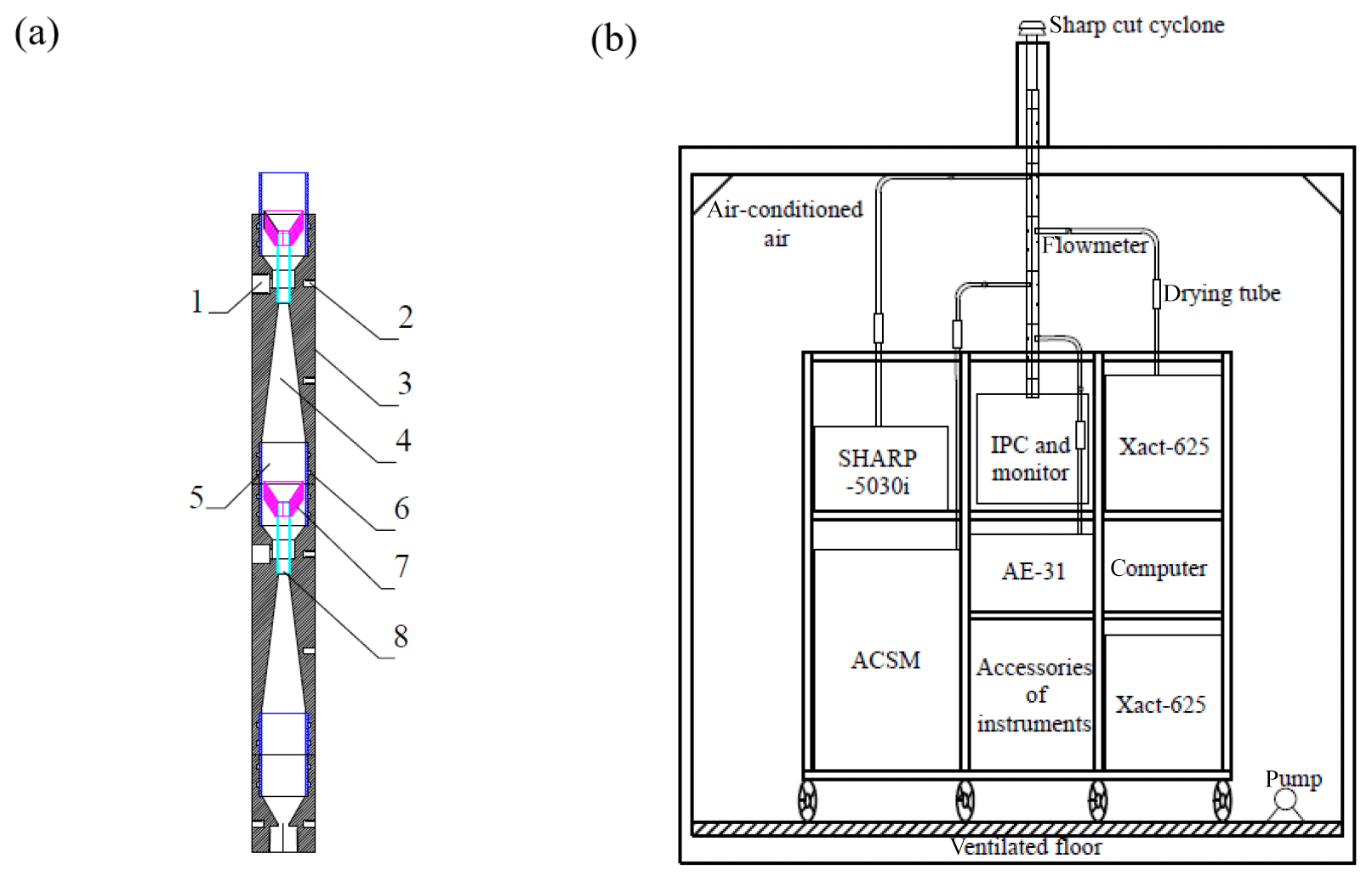
Figure 1 Structure diagram of the particle isokinetic sample tube (1 – aerosol outlet; 2 – screws for fixing; 3 – main pipe; 4 – gradual expansion channel; 5 – connecting pipe; 6 – O-ring; 7 – isokinetic sampling tube; and 8 – connecting pipe) (a). Sketch map of integrated system (IPC stands for Industrial Personal Computer) (b).

2.4 Design of the data analytics platform

To integrate online data, a data analytics platform (Fig. S2) was designed and used to export data from the integrated instruments with a uniform time resolution of 1 h, and it was also able to display the variation trends of PM_2.5 and its chemical components in real time and back up these data in an SQL server database. More details of the platform can be seen in the Supplement.

3 Application of the online integrated system

3.1 Sampling site

The sampling site was in the Peking University Shenzhen Graduate School (22^∘35^′45^′′ N, 113^∘58^′23^′′ E), which is in the western urban area of Shenzhen. Shenzhen is an international metropolis in China, surrounded by the South China Sea to the southeast and industrial cities such as Dongguan and Huizhou to the west and north. It is located in the subtropical marine climate zone, with more rainfall in summer influenced by monsoons and heavy pollution in autumn and winter due to the influence of inland air mass. The sampling site was surrounded by a large reservoir and recuperation base, with a high vegetation coverage ratio. There is no obvious pollution source except a city road about 100 m away. The measurement campaign took place from 25 September to 30 November 2019, when the pollution usually started to worsen in Shenzhen. The meteorological conditions during the campaign were shown in Fig. S3. The average ambient temperature and relative humidity were 26.7 ± 3.8^∘ and 71.9 % ± 19.0 %, respectively. The wind speed ranged from 0.1 to 6.9 m s⁻¹, with an average value of 0.6 ± 0.5 m s⁻¹. The sampling site was mainly influenced by wind from the northeast and northwest.

3.2 Sampling instruments

During the sampling period, in addition to the online integrated system, another AE-31 and MARGA system were set for independent measurements at the same site. In addition, the offline PM_2.5 measurements were simultaneously conducted every 2 d, and each sample was collected for 24 h. The sampling instruments and analytical methods of PM_2.5 chemical composition follow previous studies by Huang et al. (2018). The performance of the online integrated system was thoroughly evaluated by comparison with the measurements above.

3.3 Source apportionment modeling

3.3.1 Multilinear engine (ME-2) model

ME-2 is a factorization tool for multivariate factors, which was developed by Paatero in 1999 (Paatero, 1999). The basic principle of ME-2 can be expressed by the sample data matrix X, grouped into two constant matrices (G and F), making sure that all elements of G and F are non-negative.

$$\begin{array}{}\text{(1)}& \mathbf{X}=\mathbf{G}\cdot \mathbf{F}+\mathbf{E}\end{array}$$

G and F are the factor contribution and factor profile, respectively, which are both non-negative. E is the residual error matrix that is the difference between the measured value and the model value (Paatero and Tapper, 1994).

Table 1 Detailed constraints of the four factors used in ME-2.

The objective of the ME-2 model is to minimize the equation Q as follows:

$$\begin{array}{}\text{(2)}& Q={\sum }_{i=\mathrm{1}}^m{\sum }_{j=\mathrm{1}}^n(e_{ij}/u_{ij}{)}^{\mathrm{2}},\end{array}$$

where e_ij is the element of the matrix E and u_ij is the error and uncertainty of the measured concentration x_ij. Source Finder (SoFi) software has been developed by the Paul Schell Institute (PSI) in Switzerland, which can provide some constrained factors to realize the source constraint of ME-2 (Canonaco et al., 2013). The species uncertainties (u_ij) are estimated as follows:

$$\begin{array}{}\text{(3)}& u_{ij}=k_j\cdot x_{ij},\end{array}$$

where the x_ij is the concentration of the species and k_j is the jth species' error fraction (Huang et al., 2018), which is usually thought to be between 5 % and 30 % (Zou, 2018). Through testing, the k_j in this study was set as 20 %, and some species were expanded or decreased according to the results of model operation. When the species concentration is greater than or equal to the detection limit (DL), the uncertainty can be estimated according to the Eq. (3). Conversely, the concentration was treated by 0.5 DL and its uncertainty was set as 0.83 DL. Missing data were treated by the species' average value (geometric), and their uncertainties were assumed to be 4 times the average value.

3.3.2 Constraint setup in ME-2 modeling

SoFi was performed to initiate and control ME-2 model, and it was run for the online datasets observed by integrated system in this study. Species that satisfied one of the following conditions were excluded: (1) more than 40 % data were smaller than the DL of species, (2) less relevant to other species (r²≤0.4), and (3) low concentration that can not be used as a tracer for pollution sources. Therefore, 13 species, accounting for 98.6 % total mass concentrations of the measured species (except m/z 44), were input into the models: OM, BC, Cl⁻, ${\mathrm{NO}}_{\mathrm{3}}^{-}$, ${\mathrm{SO}}_{\mathrm{4}}^{\mathrm{2}-}$, ${\mathrm{NH}}_{\mathrm{4}}^{+}$, K, Ca, Fe, Zn, V and m/z 44.

Compared with some other interrelated studies, fragments of organic matter with m/z 44 were input into the model to track the SOA. m/z 44 is mainly composed of fragments of carboxylic acid ions ${\mathrm{CO}}_{\mathrm{2}}^{+}$, which is produced from the cracking of carboxylic acid in organic aerosols and can represent the strength of oxidation of organic aerosol (Hu, 2012). Therefore, m/z 44 was used to characterize the SOA with strong oxidization.

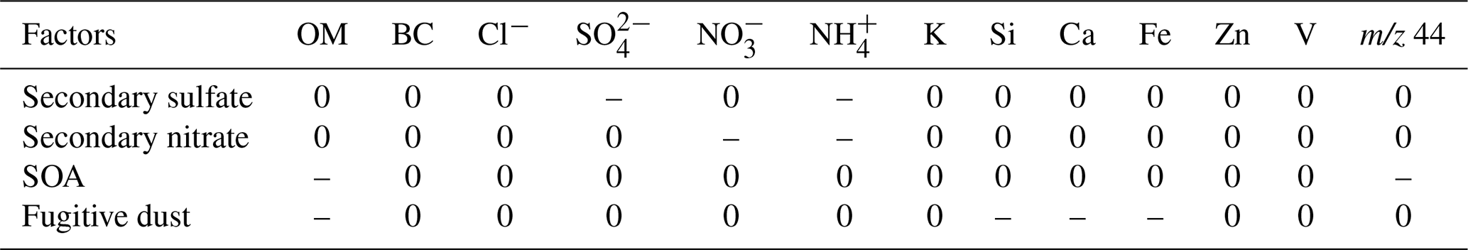
Based on the experience of our previous studies on source resolution in Shenzhen (Huang et al., 2018) and the introduction of SOA tracers, four factors were constrained as listed in Table 1: SOA, secondary sulfate, secondary nitrate and fugitive dust. For the secondary sulfate and nitrate sources, the primary source components, OM and m/z 44 in the factors were set to 0, while ${\mathrm{NH}}_{\mathrm{4}}^{+}$ and ${\mathrm{SO}}_{\mathrm{4}}^{\mathrm{2}-}$/${\mathrm{NO}}_{\mathrm{3}}^{-}$ were not limited. For the SOA, OM and m/z 44 were not limited. Based on a study of fugitive dust source profiles (Kong et al., 2011), the earth crust elements (e.g., Si, Ca, and Fe) and OM were not limited in the fugitive dust.

3.3.3 Potential source contribution function (PSCF) analysis

The PSCF was based on the analysis results of a backward trajectory, and it was used to analyze the potential regions of the possible sources of PM_2.5. Unlike the backward trajectory, which could only obtain the pathways of the air masses, PSCF can also analyze the regional transmission contribution of pollutants from different sources in the region of a given day. In TrajStat software, the movement of an air mass is described by segment endpoints of latitude and longitude coordinates (Wang et al., 2009). Before performing the PSCF analysis, the coverage area of the trajectory was 15–40^∘ N and 90–140^∘ E and the grid resolution was set to 0.4 × 0.4^∘ grid cells. The PSCF values for grid cells were calculated by the ratio of the number of contamination trajectory that were entirely in the grid cells and the number of all trajectories passing through the area. The PSCF can be defined as follows:

$$\begin{array}{}\text{(4)}& {\text{PSCF}}_{ij}={\displaystyle \frac{m_{ij}}{n_{ij}}},\end{array}$$

where i and j are latitude and longitude, respectively, PSCF_ij is the PSCF value for the ijth grid cell, m_ij represents the number of endpoints corresponding to specific source contribution above the threshold criterion, which is set to the 75th percentile of each source contribution, and n_ij represents the total number of endpoints falling in the grid cell ij.

To avoid the uncertainty caused by the limited number of endpoints in a single grid, a weight function W_ij is also considered here, as shown in Eqs. (5) and (6). For example, when the total number of trajectory endpoints in each grid (n_ij) is higher than 20 (the average endpoint) but less than 40 (4 times of average endpoint), the weighted PSCF value (WPSCF) of that grid is reduced by multiplying its original value by 0.7. The WPSCF results were used in the following discussion and called PSCF in this work.

$$\begin{array}{}\text{(5)}& {\displaystyle }& {\displaystyle }\text{WPSCF}={\text{PSCF}}_{ij}\cdot W_{ij}\text{(6)}& {\displaystyle }& {\displaystyle }{W}_{ij}=\left\{\begin{array}{llcl}\mathrm{1.00}& & & n_{ij}>\mathrm{40}\\ \mathrm{0.70}& \mathrm{20}& <& n_{ij}\le \mathrm{40}\\ \mathrm{0.42}& \mathrm{10}& <& n_{ij}\le \mathrm{20}\\ \mathrm{0.05}& & & n_{ij}\le \mathrm{10}\end{array}\right.\end{array}$$

4 Results and discussion

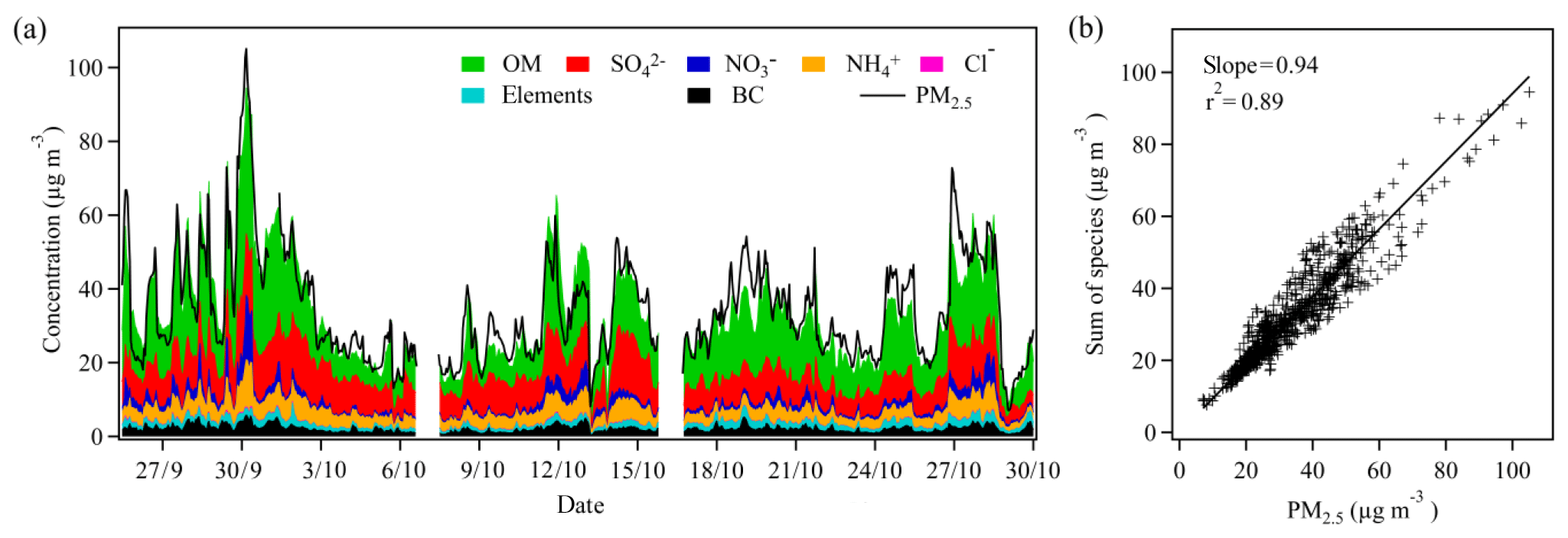
Figure 2 The trend in hourly PM_2.5 and chemical species during the sampling campaign (a). The correlation between PM_2.5 reconstructed and measured (b). Note that the term “sum of species” means the total mass concentration of chemical species from the online integrated system and that “PM_2.5” indicates mass concentration of SHARP-5030i PM_2.5.

Figure 3 Chemical compositions of average PM_2.5 during the sampling campaign.

4.1 Overview of chemical species and PM_2.5 concentrations

The time series of hourly PM_2.5 concentration and chemical species and the average concentration results are shown as Fig. 2a and Table S1 in the Supplement, respectively. Based on hourly data, PM_2.5 concentrations ranged from 5 to 107 µg m⁻³, with an average value 33 ± 14 µg m⁻³, which was lower than the Grade II national standards for air quality in China (with an annual mean of 35 µg m⁻³). OM (14.1 ± 7.4 µg m⁻³), ${\mathrm{SO}}_{\mathrm{4}}^{\mathrm{2}-}$ (8.6 ± 3.3 µg m⁻³), ${\mathrm{NO}}_{\mathrm{3}}^{-}$ (1.8 ± 1.9 µg m⁻³), ${\mathrm{NH}}_{\mathrm{4}}^{+}$ (3.8 ± 1.7 µg m⁻³) and BC (2.1 ± 1.0 µg m⁻³) were the major species, with average percentages of 41 %, 25 %, 5.3 %, 11 % and 6.4 % in PM_2.5, respectively. The major elements included Si (1.3 %), K (1.3 %), Fe (0.91 %), Ca (0.35 %), Zn (0.31 %), and the trace elements accounted for 0.84 % in PM_2.5 (Fig. 3).

4.2 Evaluation of PM_2.5 mass closure

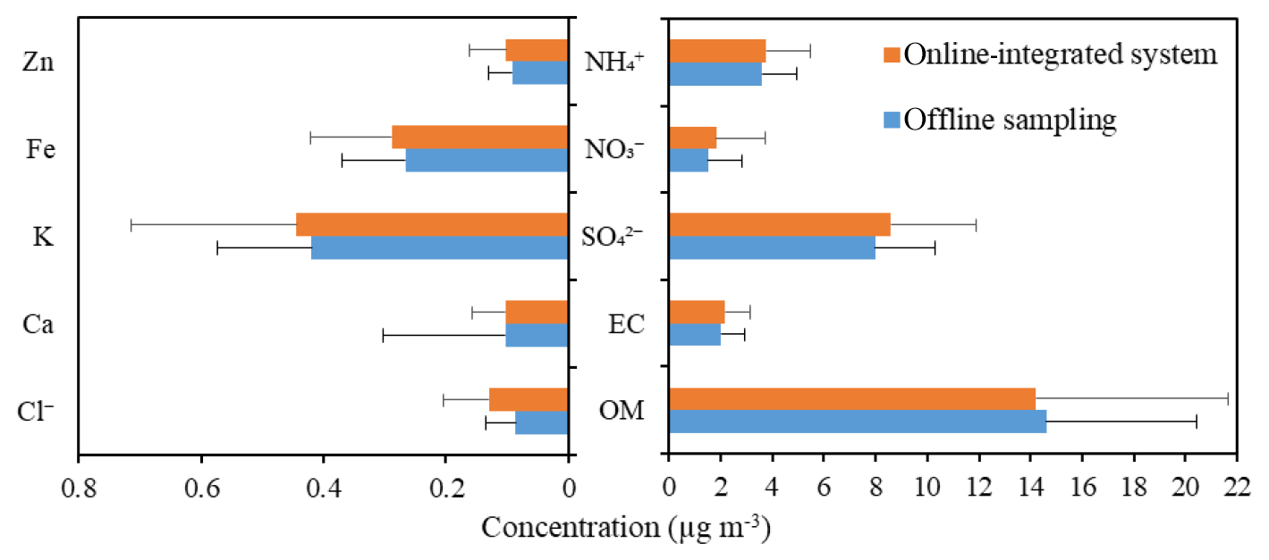
Figure 4 Concentrations of major chemical compositions of PM_2.5 measured by the online integrated system and offline sampling. Note that the EC in the online integrated system was referred to as BC.

To access the accuracies and mass closure of the receptor data from the integrated system, we reconstructed the PM_2.5 mass concentration according to the summation of chemical components. However, the correlation between the reconstructed and measured PM_2.5 mass concentration was shown as Fig. 2b. Reliable data were measured by the online integrated system and supported by the good correlation (correlation coefficient squared r²=0.89) and the slope (0.94), which was close to 1, and the results indicated that the integrated system can measure 94 % of the particulate matter components and achieve mass closure. The average error margin of mass closure during the observation period is about 6 %, which might be due to the measurement error of the integrated instruments, particle composition, temperature and relative humidity (Su et al., 2018; Zhang et al., 2017). A significant mass discrepancy between reconstructed and measured PM_2.5 appeared in some periods (Fig. 2a). For example, the underestimation on 3 October and the overestimation on 20 October occurred when the temperature was the highest and the lowest during the observation period, respectively. Therefore, it was speculated that temperature might affect the composition of PM_2.5, causing the mass closure to deviate. The online integrated system can measure more chemical components than other online instruments, for example, online continuous monitoring and analysis systems (AIM-URG9000d, USA) for water-soluble components of fine particulate, which can measure water-soluble ion contents and accounted for about 40 % of PM_2.5 mass concentrations (Han et al., 2016). A semicontinuous OC∕EC analyzer with 1 h time resolution could obtain the concentrations EC and OC, which accounted for approximately 30 % of the PM_2.5 (Liu et al., 2017). Wang et al. (2018) measured the chemical compositions using MARGA, a semicontinuous OC∕EC analyzer and Xact-625 and also reported that the sum mass concentration of measured species accounted for ∼ 78 % of PM_2.5.

4.3 Comparison with colocated measurements

The average of PM_2.5 concentrations from offline sampling was 32 µg m⁻³, which was consistent with the integrated system, and the chemical components in PM_2.5 also obtained similar results (Fig. 4), in which OM measured by online integrated and offline systems were 14.6 and 14.2 µg m⁻³, respectively, while ${\mathrm{SO}}_{\mathrm{4}}^{\mathrm{2}-}$, ${\mathrm{NO}}_{\mathrm{3}}^{-}$, and ${\mathrm{NH}}_{\mathrm{4}}^{+}$ were 7.9 %, 19.7 %, and 5.0 % higher in the online integrated system, respectively, which is possibly due to the volatilization and loss of sample during the process of offline sampling, storage and analysis. The BC measured by the online integrated system was 8.4 % higher than the EC in the offline system, and the differences of important elements were relatively small. In general, the online and offline measurements were close to each other, which indicated that the online integrated system was accurate to some extent.

Comparing the data with the results of other methods of analysis is usually used to further examine the reliability of online instruments. The BC showed high correlation with measurements of another AE-31 (r²=0.99). On average, the mass concentrations of BC measured by the integrated system report 95 % of those measured by the independent instruments (Fig. S4), suggesting the sampling model of online integrated system could avoid sampling loss effectively and was reliable. This slight underestimation of BC mass might primarily be due to the distance between sampling ports or the systematic errors between instruments.

Figure S4 shows the intercomparisons of the measurements by the ACSM with MARGA, including ${\mathrm{SO}}_{\mathrm{4}}^{\mathrm{2}-}$, ${\mathrm{NO}}_{\mathrm{3}}^{-}$, ${\mathrm{NH}}_{\mathrm{4}}^{+}$ and Cl⁻. Overall, the three ions measured by the ACSM correlated well with MARGA (r² = 0.94–0.96). The sulfate average concentrations between ACSM and MARGA were consistent (slope = 0.97). The ammonium concentrations measured by ACSM accounted for 88 % of that determined by MARGA, which might relate to the aerodynamic lens transmission efficiency of ACSM. When the particle size was less than 300 nm, the transmission efficiency was lower (Middlebrook et al., 2012). For nitrate, the ACSM measurements were approximately 64 % of what was reported by the MARGA. ACSM measured a lower Cl⁻ concentration (slope = 0.39) and a relatively poor correlation with MARGA's Cl⁻ (r² = 0.42). Another study also found a large difference between ACSM and MARGA when measuring chloride and nitrate (Zhang et al., 2017). Besides, the evaluation of PM_2.5-AMS also found a large difference in the measurements of Cl⁻ (Hu et al., 2017), which might be caused by the measuring principle of the instrument. K obtained good correlation between the Xact-625 and MARGA (r² = 0.75, Fig. S4), and the average ratio of Xact-625 to MARGA was 1.18, which might be caused by the slight difference between the K element and K⁺ in PM_2.5 as well as the differences of measurement principles. This result suggested the reliability of the Xact-625 in measuring elements.

4.4 Source apportionment analysis

4.4.1 Source apportionment results

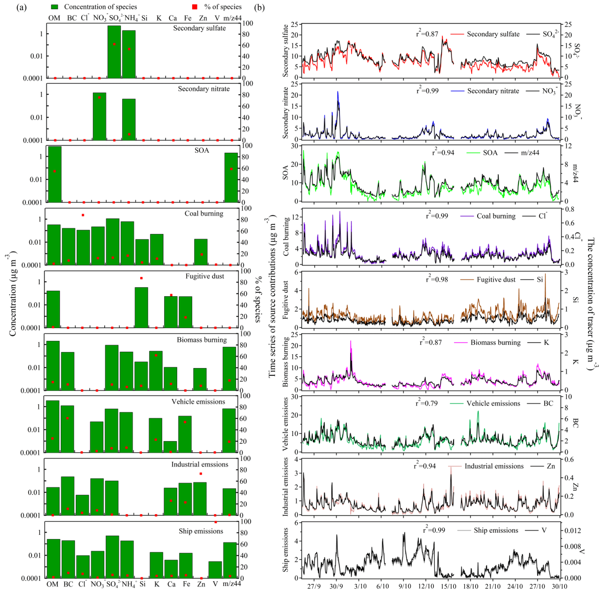
Figure 5 Factor profiles and EV in the ME-2 model results (a). Time series of PM_2.5 sources and tracers (b).

In this study, the SoFi tool was used to run the ME-2 model based on the predetermined constraints (Table 1). After the test, the RSD (relative standard deviation) of the mass concentration among each instrument was within 5 % (Q_true∕Q_exp ratio was 1.2), with the scaled residuals approximately symmetrically distributed between −3 and +3 (Fig. S5). When the factor number was less than 9, the Q_true∕Q_exp was too high, and when the factor number was more than 9, a meaningless high OM source would appear. The total mass concentration of the components (m/z 44 was not included here because it was the part of OM) input to the ME-2 model was significantly consistent with the total mass concentration of the model reconstruction (r² = 0.99, slope = 0.98).

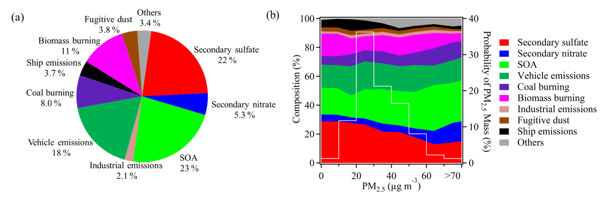
Figure 6 Average contributions of each source to PM_2.5 (a). Variation in the proportion of sources in PM_2.5 during the observation period. The white curve represents the occurrence probability of the PM_2.5 concentration (b).

Profiles of each factor were shown Fig. 5a. From top to bottom, factor 1 had large percentage of explained variation (EV) values of ${\mathrm{SO}}_{\mathrm{4}}^{\mathrm{2}-}$ and ${\mathrm{NH}}_{\mathrm{4}}^{+}$ and was identified as secondary sulfate (Huang et al., 2018). Factor 2 was related to secondary nitrate, due to significant EV values of ${\mathrm{NO}}_{\mathrm{3}}^{-}$ and ${\mathrm{NH}}_{\mathrm{4}}^{+}$ (Huang et al., 2018). Factor 3 was identified as SOA, which has a significant EV value of m/z 44 and OM, m/z 44 had high concentration in this factor, thus suggesting it is a good tracer of SOA. Previous studies tried to identify SOA using receptor models and indicated SOA mixed with secondary sulfate and/or secondary nitrates due to the lack of tracer (Huang et al., 2018); in this study, the effective tracer of SOA was introduced into the model, resulting in the SOA being identified separately. Factor 4 was associated with coal burning due to the high EV value of Cl⁻, which is formed by the rapid combination of HCl and ammonia in the atmosphere. The potential source of HCl is coal burning in China (Yudovich and Ketris, 2006; Wang et al., 2015), and the concentration distribution of Cl⁻ in the Pearl River Delta was consistent with the distribution of coal-fired power plants in the source list (Huang et al., 2018). This factor also had some mass contributions from ${\mathrm{SO}}_{\mathrm{4}}^{\mathrm{2}}$, ${\mathrm{NO}}_{\mathrm{3}}^{-}$, and EC, further confirming that it was from coal burning. Factor 5 was explained as fugitive dust due to its high EV values of Si and Ca, which came from the earth's crust and building dust, respectively (Amil et al., 2016). The integrated system does not involve the measurement of oxygen (O) and Al. Instead, the contents of O and Al in factor 5 were estimated indirectly based on the abundance of the three (Al, O, Si) in the crust. (Taylor and Mclennan, 1995). Factor 6 has a high loading of K and a certain amount of OM and BC. K has been used as a clear tracer for biomass burning (Yamasoe et al., 2000; Sillapapiromsuk et al., 2013). Biomass burning is a significant source of PM_2.5 and organic matter in China. The Zn contained in this factor might be related to garbage-burning (Yuan et al., 2006). Besides, biomass burning has a high contribution from the north and southwest (Fig. 8), which is consistent with the distribution of fire points in Guangdong (Fig. S6). The activities of biomass burning often occur during the daytime, which is consistent with the diurnal pattern of biomass burning that has high daytime and low nighttime concentrations (Fig. 7). Factor 7 was identified as vehicle emissions due to the high concentrations of OM and BC related to oil combustion. This factor also showed certain loadings of Fe might come from tires and brake wear of vehicles (He et al., 2011; Yuan et al., 2006). Factor 8 displayed large EV values of Zn, and Fe and Ca also had high enrichment factors. The Zn might have been due to industrial sources, such as plastic incineration, coating and metallurgy (Zabalza et al., 2006; Cruz Minguillón et al., 2007). The Ca might come from the soot produced by the inferior coal and diesel combustion in the industry (Lewis and Macias, 1980). The Fe might be related to ceramic production (Querol et al., 2007) and was thus considered to be related to industrial processes. Factor 9 was ship emissions, due to a large EV values of V. V is mainly produced by burning of heavy oil, which is used as fuel by ships in the port of Shenzhen (Huang et al., 2014). The factor of sea salt cannot be identified in this study, because the measurement of its tracer (Na) is limited for the X-ray fluorescence method and ACSM. However, the contribution of sea salt is low for Shenzhen (about 1 % to 3 %) and is not the main source of pollution. The high time resolution of source contributions could be output when source apportionment was performed using online datasets. Fig. 5b shows the time series of each source, as well as their corresponding tracers during source resolution in Shenzhen. The sources had a very good correlation with the tracer species (r² = 0.79–0.99), suggesting that the model could identify representative pollution factors. Compared with primary sources, secondary sources fluctuate more dramatically with time. Among all the sources, the trend of secondary sulfate was closer to PM_2.5, reflecting that it was the one of the main contributors to PM_2.5.

Figure 7 Diurnal variations of the nine sources resolved by ME-2.

Figure 6a showed the average contributions of the PM_2.5 sources during the sampling period. It can be seen that the SOA, secondary sulfate, vehicle emissions and biomass burning were the main sources in Shenzhen, contributing 23 %, 22 %, 18 % and 11 % of PM_2.5 mass concentration, respectively. The total contribution above four sources was more than 70 %. The contributions of the other sources were smaller (2 %–8 %) and from large to small were coal burning (8 %), secondary nitrate (5.3 %), fugitive dust (3.8 %) and ship emissions (3.7 %). The unidentified sources accounted for 3.4 %, which was caused by a combination of residuals from ME-2 model and measurement deviations of integrated system.

As shown in Fig. 6b, the contribution change of PM_2.5 factors was analyzed with the change of total PM_2.5 concentration. Secondary sulfate and biomass burning decreased when pollution was heavy, while the secondary nitrate and SOA increased. Therefore, secondary conversion of carbon-containing and NO_x components were the causes of heavy PM_2.5 pollution during the observation period.

4.4.2 Diurnal variations

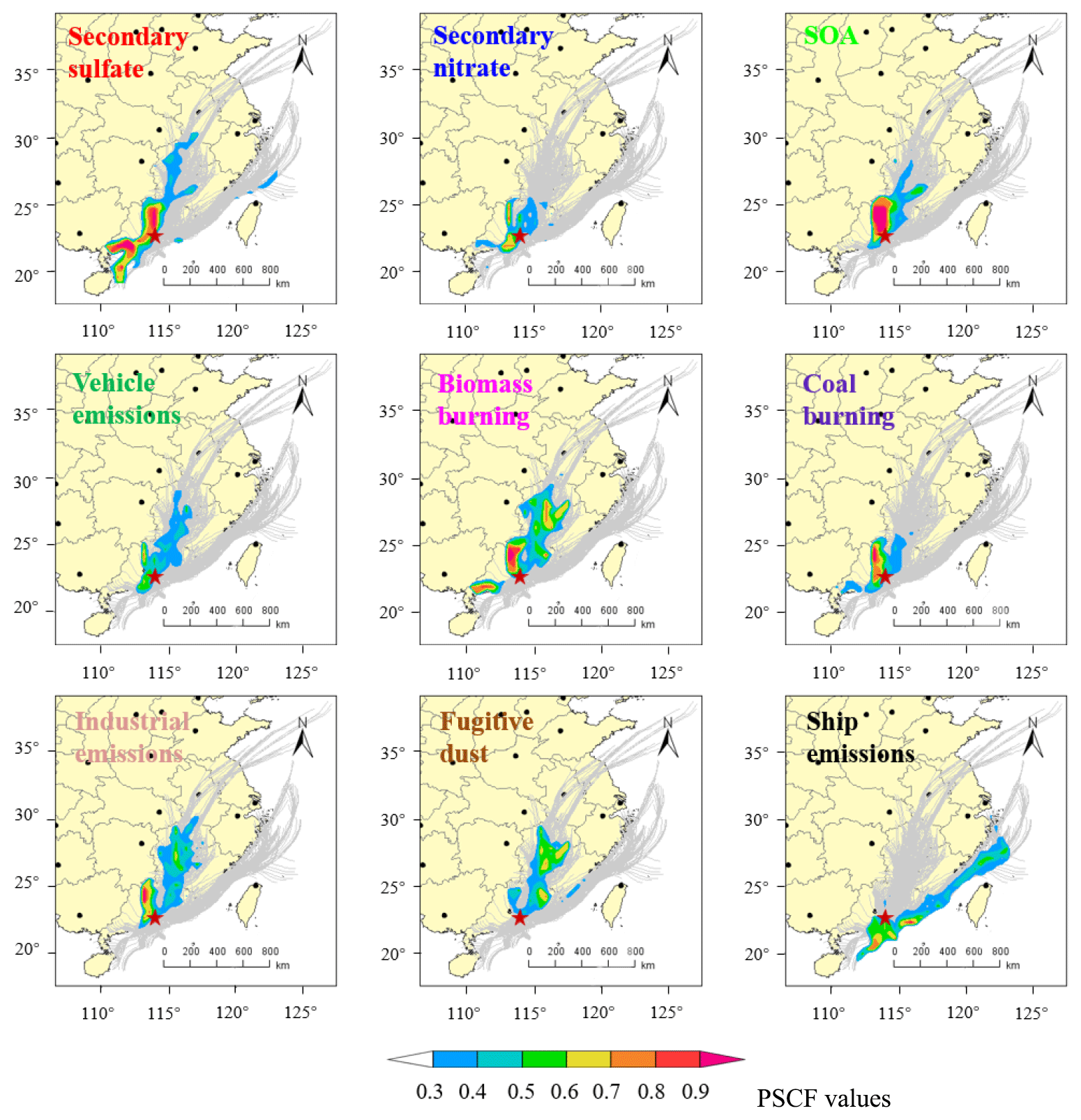
Figure 8 Spatial distributions of PSCF values for the nine sources resolved by ME-2.

Diurnal variations of source were obtained based on the high time resolution data, which could help to evaluate the validity of the source apportionment and investigate the causes of PM_2.5 pollution further. The average diurnal trends of major sources are shown in Fig. 7. Secondary sulfate diurnal variations presented relatively high afternoon concentrations and low nighttime concentrations; moreover, a broad peak from 12:00 to 20:00 UTC+8 might be related to light intensity, suggesting that sulfate was largely formed by photochemical processes (Liu et al., 2008). In contrast, secondary nitrate had a peak during 09:00–10:00 UTC+8 that was slightly later than the morning rush hour for motor vehicles because the NO_x in vehicle exhaust was an important source of secondary nitrate. The pattern (high nighttime concentration and low afternoon concentration) might be caused by the diurnal variation of the boundary layer. Decreasing solar activity at night resulted in the height of boundary layer decreasing and the inversion layer occurring. (Xu et al., 2014), which was not conducive to the diffusion of pollutants. Moreover, the pattern might be due to the evaporation of ammonium nitrate produced by the secondary reaction at high temperatures in the afternoon. The variation of SOA was related to the photochemical reaction of volatile organic compounds. When the sun rises during the day, the boundary layer was gradually elevated, which led to lower concentrations of residual SOA in the atmosphere, and it reached its lowest point between 08:00 and 09:00 UTC+8. After that, SOA rose and peaked at 14:00 UTC+8 due to the enhancement of light. It was consistent with the theoretical changes in SOA (Liu et al., 2018). For primary sources, vehicles, ships and industrial emissions showed the characteristics of ”two peaks and one valley”, which were basically consistent with the law of human activities. This finding suggested that human activities have a significant impact on environmental pollution. Biomass burning and fugitive dust showed a trend of high daytime and low nighttime concentrations, which might be because of the local emissions (such as biomass boiler or construction activities) during daytime being mixed with the pollutants transported from other regions due to the rise of boundary layer at morning (Sun et al., 2019). Analyzed with the time series of pollution sources (Fig. 5b), the results showed that the peaks around 22:00 and 01:00 UTC+8 for biomass burning were mainly due to the abnormally high source contribution on the night of October 1, which is China's National Day, and because there were displays of fireworks from 25 September to 1 October at three playgrounds 10 km away from sampling site. Previous study has shown that the concentration of species (e.g., K, Ca, Cl⁻, ${\mathrm{NO}}_{\mathrm{3}}^{-}$) in the PM_2.5 would have greatly increased due to the fireworks (Tsai et al., 2012). The spike at 01:00 UTC+8 of fugitive dust and biomass burning was mainly caused by several abnormally high values at that time, suggesting it might be due to the influence of local short-term activities. The daily variation of coal burning and Cl⁻ was consistent (Fig. S7), and there is a peak around 09:00 UTC+8. This might be because the temperature starts to rise in the morning and the vertical air convection activity is strengthened, bringing the pollutants transmitted by overhead sources to near the ground. The spike around 22:00 UTC+8 was mainly because of firework shows from 25 September to 1 October. The peak around 14:00 UTC+8 mainly came from local sources on 25 September. Diurnal variations of each source were more consistent with the actual situation, which indicated that the results of source apportionment were reasonable.

4.4.3 Potential source areas

The potential source areas for different sources were identified by the PSCF model as shown in Fig. 8. During the observational campaign, Shenzhen City was mainly influenced by the continental and coastal air masses coming from the northeast of the domain and, to a lesser extent, by the air masses originating from southwest of the city. The continental air masses transported from the north of Guangdong Province, Jiangxi Province and the Yangtze River Delta region, where there are highly urbanized and industrialized areas. The coastal air masses stem from the East China Sea and Taiwan Strait. The secondary sulfate showed two potentially important source areas located to the north and southwest of the sampling site. The southwestern potential source areas indicated that regional influences were important to the secondary sulfate. Compared with secondary sulfate, the high potential source region of secondary nitrate was closer to the sampling site and mainly located in the southwestern and northern areas. These findings implied that secondary nitrate was from local secondary aerosol rather than regional transport. The PSCF plot of SOA displayed a clear high potential source region in northern Guangdong Province, including the cities of Dongguan, Huizhou and Shaoguan. The PSCF plot of vehicle emissions showed potential source areas around the sampling site. Fugitive dust and biomass burning have a similar potential source region, originating from the northeastern area of the site, suggesting the two sources may be influenced by the regional transport. This result was consistent with the high fugitive dust and biomass burning contributions to PM_2.5 during daytime, which are partly related to regional transport (Fig. 7). Sun et al. (2019) conducted vertical observations of air pollutants (SO₂, O₃, NO_x, PM₁₀, PM_2.5) and revealed the obvious regional transport in Shenzhen. In addition, biomass emission also showed high potential source regions in the northern area Guangdong Province. The PSCF plot of biomass burning indicates local emissions and regional influences. Coal-burning high potential source areas were similar but smaller compared to those of industrial emissions, which were mainly located in the northern area of Shenzhen. The potential areas of ship emissions were consistent with the coastal regions, where there are many shipping ports, especially the Shenzhen ports, which are the third largest in the world and have active shipping lanes with traffic volumes up to 500 000 transits in 2015 (Mou et al., 2019). In summary, the PSCF analysis indicated that the northern domain was the high potential source region for secondary aerosol, coal burning, and industrial emissions. Vehicle emissions and secondary nitrate were mostly influenced by local emissions. For fugitive dust, biomass burning, ship emissions, and secondary sulfates, the potential source areas on a regional scale were important in this study.

5 Conclusions

In this work, a new online integrated system for the measurement of chemical species in PM_2.5 was developed by combining ACSM, Xact-625, AE-31 and SHARP-5030i. A sampling tube was designed to reduce aerosol transmission loss. Approximately 94 % of PM_2.5 components can be detected, and the data (except Cl⁻) were well correlated with those measured by other independent online instruments (MARGA, AE-31), with r² values ranging from 0.74 to 0.99. The concentrations of chemical components were similar to those of offline sampling. To more accurately reveal the PM_2.5 pollution characteristics, the new online integrated system was applied at the university area of Shenzhen in the autumn of 2019. The average PM_2.5 concentration was 33 µg m⁻³ during the sampling period, of which ${\mathrm{SO}}_{\mathrm{4}}^{\mathrm{2}-}$, OM, ${\mathrm{NH}}_{\mathrm{4}}^{+}$, BC, ${\mathrm{NO}}_{\mathrm{3}}^{-}$, important elements and Cl⁻ contributed 25 %, 41 %, 11 %, 6.4 %, 5.3 %, 5.0 % and 0.38 %, respectively. The chemical composition measured was close to the mass closure.

An improved source apportionment method was established by employing the ME-2 model on the mass spectra information (m/z 44) and chemical species measured from the online integrated system to solve the SOA contributions. SOA was found to be the dominant source (23 %), followed by secondary sulfate (22 %), vehicle emissions (18 %), biomass burning (11 %), coal burning (8.0 %), secondary nitrate (5.3 %), fugitive dust (3.8 %), ship emissions (3.7 %) and industrial emissions (2.1 %). The online integrated systems applied for source apportionment could obtain more accurate results through the analysis of time series trend and diurnal variation. The emission source had high correlation with the tracer species (r² = 0.79–0.99). Secondary sulfate and SOA showed high concentrations during the daytime, which was associated with photochemical processes. The concentration of secondary nitrate was high at nighttime and low in the afternoon, and the variation of primary sources was basically consistent with the law of human activities, indicating that the results of source apportionment were reasonable. The results of the PSCF model indicated that the northern area of the sampling site was the potential source region during the sampling campaign and regional transmission (e.g., biomass burning, fugitive dust, etc.) and also played an important role in PM_2.5 pollution in this work. The development and successful application of the online integrated system and source apportionment method suggested that they can be used for precise regulation of PM_2.5. The high time resolution source analysis of the new integrated system is helpful for the study of the variation of the primary and secondary sources of PM_2.5 in the process of heavy pollution (such as fireworks) and to identify the key sources and its mechanisms, which can then be used to assess the impact of different sources. The system can run stably for a long time and provides a key scientific basis for particulate matter control of China.