A new method to correct the electrochemical concentration cell (ECC) ozonesonde time response and its implications for “background current” and pump efficiency

The electrochemical concentration cell (ECC) ozonesonde has been the main instrument for in situ profiling of ozone worldwide; yet, some details of its operation, which contribute to the ozone uncertainty budget, are not well understood. Here, we investigate the time response of the chemical reactions inside the ECC and how corrections can be used to remove some systematic biases. The analysis is based on the understanding that two reaction pathways involving ozone occur inside the ECC that generate electrical currents on two very different timescales. The main fast-reaction pathway with a time constant of about 20 s is due the conversion of iodide to molecular iodine and the generation of two free electrons per ozone molecule. A secondary slow-reaction pathway involving the buffer generates an excess current of about 2 %–10 % with a time constant of about 25 min. This excess current can be interpreted as what has conventionally been considered the “background current”. This contribution can be calculated and removed from the measured current instead of the background current. Here we provide an algorithm to calculate and remove the contribution of the slow-reaction pathway and to correct for the time lag of the fast-reaction pathway.

This processing algorithm has been applied to ozonesonde profiles at Costa Rica and during the Central Equatorial Pacific Experiment (CEPEX) as well as to laboratory experiments evaluating the performance of ECC ozonesondes. At Costa Rica, where a 1 % KI, 1/10th buffer solution is used, there is no change in the derived total ozone column; however, in the upper troposphere and lower stratosphere, average reported ozone concentrations increase by up to 7 % and above 30 km decrease by up to 7 %. During CEPEX, where a 1 % KI, full-buffer solution was used, ozone concentrations are increased mostly in the upper troposphere, with no change near the top of the profile. In the laboratory measurements, the processing algorithms have been applied to measurements using the majority of current sensing solutions and using only the stronger pump efficiency correction reported by Johnson et al. (2002). This improves the accuracy of the ECC sonde ozone profiles, especially for low ozone concentrations or large ozone gradients and removes systematic biases relative to the reference instruments.

In the surface layer, operational procedures prior to launch, in particular the use of filters, influence how typical gradients above the surface are detected. The correction algorithm may report gradients that are steeper than originally reported, but their uncertainty is strongly influenced by the prelaunch procedures.

1 Introduction

The electrochemical concentration cell (ECC) ozonesonde is one of the most important instruments for the measurement of vertical profiles of ozone and is used in a number of important networks, e.g., the ozonesonde network of Global Atmosphere Watch (GAW), the Southern Hemispheric Additional Ozonesondes (SHADOZ), and the Network for the Detection of Atmospheric Composition Change (NDACC). It provides observations of high fidelity and high vertical resolution, which among others are considered a reference for satellite-based remote-sensing observations. Its operation has been described in detail elsewhere (e.g., Komhyr, 1969; Komhyr and Harris, 1971; Smit and ASOPOS panel (2014); Sterling et al., 2018; Tarasick et al., 2020).

The ECC generates an electrical current through the reaction of ozone in a potassium iodide (KI) solution, which produces approximately two electrons per molecule of ozone. The ozone partial pressure ($P_{{\mathrm{O}}_{\mathrm{3}}})$ is then calculated using the ECC equation:

$$\begin{array}{}\text{(1)}& P_{{\mathrm{O}}_{\mathrm{3}}}=c\cdot T\cdot t_{\mathrm{100}}\cdot \mathit{\gamma }\cdot I_{{\mathrm{O}}_{\mathrm{3}}},\end{array}$$

where $P_{{\mathrm{O}}_{\mathrm{3}}}$ is in millipascals; $I_{{\mathrm{O}}_{\mathrm{3}}}$ in microamperes is the cell current attributed to the reaction of ozone with iodide; $c=\mathrm{4.309}\times {\mathrm{10}}^{-\mathrm{4}}$ is the ratio of the ideal gas constant and Faraday constant divided by the yield ratio of two electrons per ozone molecule; T in kelvin is the air temperature entering the cell, approximated by the temperature of the pump; t₁₀₀ in seconds is the flow rate time to pump 100 mL; and γ is a pressure-dependent pump flow correction factor. Other efficiency corrections may be included in γ (e.g., Witte et al., 2017; Sterling et al., 2018; Tarasick et al., 2020) but are omitted here for simplicity.

Throughout the ECC ozonesonde community, these instruments are operated using predominantly three chemical solution recipes; these differ mostly in the relative concentration of the potassium iodide and the concentration of the buffer (see Johnson et al., 2002). The original solution recipe introduced by Komhyr (1986) is referred to as the 1 % KI, full-buffer solution and has been used in many ozone soundings including those during the Central Equatorial Pacific Experiment (CEPEX; Kley et al., 1996; Vömel and Diaz, 2010, hereafter VD2010). When it was understood that the buffer in these solutions not only regulates the pH value but also contributes to the generation of excess electrons, Komhyr (EN-SCI, 1996) proposed to dilute the original recipe by a factor of 2. This recipe is referred to as the 0.5 % KI, half-buffer solution. Sterling et al. (2018) introduced a third solution, in which only the strength of the buffer was reduced by a factor of 10 while maintaining the original concentration of potassium iodide. This solution will be referred to as 1 % KI, 1/10th buffer solution and has been used across the NOAA ozonesonde network as well as in Costa Rica.

The pump flow correction factor compensates for a reduced pump efficiency at low pressure, which becomes relevant at pressures less than 100 hPa, i.e., in the stratosphere. Three pump flow correction tables are currently in widespread use (Komhyr, 1986; Komhyr et al., 1995; Johnson et al., 2002; see Smit and ASOPOS panel, 2014, for more details), which in the middle stratosphere (10 hPa) differ by as much as 10 %. The pump flow corrections by Komhyr (1986) and Komhyr et al. (1995) are recommended for sondes using the more strongly buffered solutions (1 % KI, full-buffer, and 0.5 % KI, half-buffer respectively). The pump flow correction by Johnson et al. (2002), which provides a stronger correction than the other two, is recommended only for sondes using the 1 % KI, 1/10th buffer solution. By pairing these recommendations, systematic biases due to the generation of excess electrons in a particular sensing solution have historically been compensated by the matching pump efficiency correction. However, only the pump flow correction by Johnson et al. (2002) currently describes the true loss of pump efficiency and is consistent with measurements from other groups (Tatsumi Nakano, personal communication, 2018). Pairing this pump efficiency with the more strongly buffered solutions leads to an overestimation of stratospheric ozone.

Prior to launch on a meteorological sounding balloon, ECC ozonesondes are prepared largely following standard operating procedures, which are described in GAW report 201 (Smit and ASOPOS panel, 2014) and which are currently under review. A central step during the preparation of the ECC is the exposure of the cell to defined amounts of ozone, typically for 5 min. The amount of ozone is regulated such that the cell generates an electrical current of 5 µA. After ozone exposure, air free of ozone is pumped through the cell and the decay of the cell current is measured. Typical parameters measured are the time during which the cell current drops from 4 to 1.5 µA (about 20 s), and the cell current 10 min after exposure to ozone has ended (typical values in the range of about 0.01 to 0.05 µA). In addition, the time the pump takes to sample 100 mL air is measured.

Commonly, a “background current” I_B is subtracted from the measured cell current I_m to obtain the current attributed to the reaction of ozone with iodide:

$$\begin{array}{}\text{(2)}& I_{{\mathrm{O}}_{\mathrm{3}}}=I_{\mathrm{m}}-I_{\mathrm{B}}.\end{array}$$

This background current has been assumed to be the cell current in the absence of ozone and is a major contribution to the uncertainty of ozone measurements, particularly in the tropical upper troposphere and in the boundary layer of clean regions of our atmosphere, where ozone concentrations are low (Witte et al., 2018; Tarasick et al., 2020). I_B is treated as a constant offset from the measured current throughout the profile and is measured multiple times as part of the standard operating procedures; however, there are inconsistencies about which of these measurements should be used as the final I_B in Eq. (1). In current data records, I_B may have been taken as the cell current prior to the conditioning of the cell with ozone (IB0), as the cell current 10 min after conditioning (IB1), as the cell current using an ozone destruction filter just before launch (IB2), or as a constant value used for all sondes. A decaying background, recommended by one sonde manufacturer (SPC, 2014), is less well defined and has caused additional ambiguity in processing and interpreting of ozonesonde observations. The arbitrary nature of this term introduces uncertainty that is difficult to quantify. Here, we investigate how the temporal response of the ECC controls the background current and how this may be used to improve the processing of ECC ozonesonde measurements.

VD2010 studied the cell current during preparation of the ECC in more detail and pointed out that the concept of a constant background is not supported by the behavior of the instrument during preparation. After exposure to ozone, the measured cell current continues to decrease with a slow time constant of about 25 min. Although the absolute value of the cell current during this decrease differs between the three different solutions, the slow rate of decay of the cell current after ozone exposure is similar for these three solution types. In none of their tests was a constant level established that could be justifiably used as constant background in the calculation of the ozone partial pressure.

VD2010 also pointed out that for many field stations, the availability of ozone-free air is limited. Purified air using ozone destruction filters are most commonly used at both operational and campaign-driven sites. It cannot be assumed that these filters operate with perfect efficiency and under all conditions (Reid et al., 1996; Newton et al., 2016; Witte et al., 2017). Therefore, the measurement of the cell current after the exposure to ozone using such filters may still include some contribution from the reaction of residual ozone and iodide, further complicating the determination of a background current.

Here, we argue that the term “background current” is a misnomer and suggest that the term “postpreparation current” is more suitable, tying this term to the standard operating procedures and referring explicitly to the cell current measurement 10 min after the exposure of ozone. This preparation current provides valuable information about the functionality of the sensor and connects to the established record of ECC operations over the past 50 years.

VD2010 emphasized the role of side reactions of the buffer with ozone and the time dependence of the different reaction pathways, which may generate electrical currents in excess of the conversion efficiency of 2. Tarasick (2020) proposed considering the different reaction pathways explicitly and deriving a quantitative method linking the slow side reactions to what has historically been called the background current. Here, we explore this proposal further and evaluate a quantitative algorithm, which takes into account the slow-reaction path involving the buffer as well as a correction for the time response delay of the fast-reaction path in the reaction between ozone and iodide.

The time response of the ECC has been studied in the past. De Muer and Malcorps (1984) studied the frequency response of Brewer–Mast type electrochemical ozonesondes, which is based fundamentally on a similar chemistry as the ECC. They recognized that a convolution of different frequency responses is required to correct the time response of that sonde type. Imai et al. (2013) applied a correction for the fast-reaction pathway for the validation of Superconducting Submillimeter-Wave Limb-Emission Sounder (SMILES) satellite observations. Huang et al. (2015) derived a different correction for the fast-reaction pathway, which in effect is very similar to that applied by Imai. However, none of the previous studies considered the time response of the slow- and fast-reaction pathways and their connection to the background current as well as the fact that these processes require the use of a proper pump efficiency correction to avoid a compensation of biases.

We argue that the preparation current should not be used in the calculation of the ozone partial pressure and that its role is replaced by the explicitly calculated contribution of the slow-reaction path. This contribution combined with correcting for the response time lag of the fast reaction and using a proper pump efficiency correction better accounts for the generation of excess electrons by the more strongly buffered solutions.

In the calculation of the total ozone column, we use the satellite climatology by McPeters and Labow (2012) to estimate the amount of ozone not measured by the ECC above the balloon burst or above 10 hPa, whichever comes first. Using this climatology and the limit of 10 hPa for the top of the ozonesonde profile reduces the influence of the strongest pump efficiency correction near the top of the profile.

2 Method

VD2010 showed that the decay of the ECC cell current after the exposure of ozone in the laboratory can be described by the superposition of two exponential decay functions:

$$\begin{array}{}\text{(3)}& I_{\mathrm{m}}=I_{\mathrm{f}}+I_{\mathrm{s}},\end{array}$$

where I_f is the instantaneous contribution of the fast reaction with a time constant of τ_f≈20 s, and I_s is the contribution of the slow reaction with a time constant of τ_s≈25 min.

The fast term is due to the reaction of ozone with potassium iodide and constitutes about 90 %–98 % of the measured cell current. Komhyr (1969) and Komhyr and Harris (1971) attribute its time constant to diffusive transport of iodine through the diffusion layer to the cathode electrode. They report a time constant of faster than 20 s at 25 ^∘C with a strong temperature dependence and a slowing to 40 s at 2 ^∘C.

Saltzman and Gilbert (1959) and Flamm (1977) attribute the slow-reaction path to additional reactions involving the neutral phosphate buffer used in the sensing solutions. Flamm (1977) determined a time constant of 27.4 min; Tarasick et al. (2020) use a time constant of 20 min for the slow-reaction path.

The decay of the cell current signal differs in magnitude between the two solution recipes studied by VD2010, even though the time constants for the two solution recipes are very similar. Therefore, we concluded along with others (e.g., Johnson et al., 2002) that the concentration of the buffer is the main cause for the different responses. This also implies that the different solution recipes may be handled mathematically in the same way but differingly in some parameters.

Only the current I_f generated in the fast primary reaction with iodide should be used in the calculation of the ozone partial pressure in Eq. (1). In contrast, the current contribution I_s generated from the slow secondary reactions must be considered as an excess current that should be subtracted from the measured cell current. Therefore, the term, which in the past has been considered a constant background current, should rather be considered a time-dependent excess current due to the secondary reactions within the ECC.

To understand the partitioning between the two reaction pathways, we can first analyze the slow-reaction pathway separately since its time constant is about 75 times larger than that of the fast reaction. The time dependence of the exponential decay can be written as

$$\begin{array}{}\text{(4)}& {\displaystyle \frac{\mathrm{d}{I}_{\mathrm{s}}}{\mathrm{d}t}}=-{\displaystyle \frac{\mathrm{1}}{{\mathit{\tau }}_{\mathrm{s}}}}(I_{\mathrm{s}}-I_{\mathrm{s},\mathrm{ss}}),\end{array}$$

where I_s,ss is the steady state of the slow reaction at any moment in the ozone profile. This can be integrated over short time periods during which the steady-state value of the slow reaction can be considered constant:

$$\begin{array}{}\text{(5)}& I_{\mathrm{s}}\left(t\right)=\left(\mathrm{1}-e^{-\frac{t-t_{\mathrm{0}}}{{\mathit{\tau }}_{\mathrm{s}}}}\right)\cdot I_{\mathrm{s},\mathrm{ss}}+e^{-\frac{t-t_{\mathrm{0}}}{{\mathit{\tau }}_{\mathrm{s}}}}\cdot I_{\mathrm{s}}\left(t_{\mathrm{0}}\right).\end{array}$$

This equation can be evaluated iteratively over all time steps of a profile beginning with the start of data recording prior to launch. Doing so requires some knowledge of the slow-pathway contribution at the beginning of data recording I_s(t₀=0) and some understanding of the steady state of the slow reaction.

If an ozone destruction filter was used as part of the launch preparation procedures, then the cell current reading at t₀ = 0, i.e., the moment just before the filter was removed (IB2), is equivalent to the slow-reaction pathway only. Without the use of an ozone destruction filter, a slow-pathway contribution I_s(t₀=0) must be assumed. The influence of the slow-reaction pathway at the surface I_s(t₀=0) decreases exponentially as the sounding progresses and justifies abandoning the concept that IB2 or any other arbitrary value should be applied as constant background throughout the profile.

After removing the ozone destruction filter before launch or after the conclusion of the ECC preparation, the measured cell current becomes the superposition of both pathways. The uncertainty in the development of the slow pathway prior to launch is the largest contribution to the uncertainty of the measurements in the boundary layer but decreases as the contribution of the prelaunch reading decreases. Variations in operational procedures, such as when the ozone destruction filter is removed, and time elapses between the end of the ozone conditioning and launch, contribute to the uncertainty.

At the same time, the contribution of the slow-pathway steady-state I_s,ss increases. The value of this steady state cannot be measured directly during a sounding and has to be determined in laboratory experiments. VD2010 measured the excess cell current as a function of cell current under steady-state conditions for the three solution recipes and determined a linear relationship between the excess and the measured cell current (their Fig. 4). Their measurements showed that the steady-state contribution of the slow-reaction pathway is directly proportional to the measured cell current, i.e., I_f≈αI_m. This can be used to write Eq. (5) as

$$\begin{array}{}\text{(6)}& I_{\mathrm{s}}\left(t\right)=\left(\mathrm{1}-e^{-\frac{t-t_{\mathrm{0}}}{{\mathit{\tau }}_{\mathrm{s}}}}\right)\cdot \mathit{\alpha }\cdot I_{\mathrm{m}}\left(t\right)+e^{-\frac{t-t_{\mathrm{0}}}{{\mathit{\tau }}_{\mathrm{s}}}}\cdot I_{\mathrm{s}}\left(t_{\mathrm{0}}\right).\end{array}$$

VD2010 derived steady-state bias factors of $\mathit{\alpha }=\mathrm{0.090}\pm \mathrm{0.005}$ for the 1 % KI, full-buffer solution; $\mathit{\alpha }=\mathrm{0.031}\pm \mathrm{0.004}$ for the 1 % KI, 1/10th buffer solution; and $\mathit{\alpha }=\mathrm{0.024}\pm \mathrm{0.009}$ for the 0.5 % KI, half-buffer solution.

Equation (6) allows an iterative calculation of the contribution of the slow-reaction pathway using the time constant τ_s≈25 min, the measured cell current, and an assumed or measured slow-reaction pathway cell current I_s(t₀=0) prior to launch. The iteration preferably starts with prelaunch measurements but in practice may be limited to calculations starting at launch. In that case, the uncertainty of the initial slow-reaction pathway may be significant, depending on the amount of ozone in the near-surface boundary layer.

With that knowledge of the slow-reaction pathway, we can now evaluate the response of the fast-reaction pathway and remove its time lag, which is introduced by the response time of about 20 s. After removing the contribution of the slow reaction from the measured cell current, we can write the fast-reaction contribution as

$$\begin{array}{}\text{(7)}& I_{\mathrm{f}}\left(t\right)=I_{\mathrm{m}}\left(t\right)-I_{\mathrm{s}}\left(t\right).\end{array}$$

Its time response can be written similarly to that of the slow reaction as

$$\begin{array}{}\text{(8)}& {\displaystyle \frac{\mathrm{d}{I}_{\mathrm{f}}\left(t\right)}{\mathrm{d}t}}=-{\displaystyle \frac{\mathrm{1}}{{\mathit{\tau }}_{\mathrm{f}}}}\left(I_{\mathrm{f}}-I_{\mathrm{f},\mathrm{ss}}\right),\end{array}$$

where I_f,ss is the steady state of the fast reaction at any moment in the ozone profile. The contribution of the fast-reaction I_f to the measured cell current I_m is subject to time lag, whereas the instantaneous steady-state I_f,ss represents the fast-reaction cell current that would be measured if the ozone concentration was in a steady state. Equation (8) can be rearranged to

$$\begin{array}{}\text{(9)}& I_{\mathrm{f},\mathrm{ss}}=I_{\mathrm{f}}+{\mathit{\tau }}_{\mathrm{f}}\cdot {\displaystyle \frac{\mathrm{d}{I}_{\mathrm{f}}}{\mathrm{d}t}}.\end{array}$$

This equation is identical to the equation derived by Huang et al. (2015) and removes a small bias in the fast-reaction pathway due to its time constant of approximately 20 s. For small time steps dt≪τ_f, this is also equivalent to the equation used by Imai et al. (2013). The steady-state cell current I_f,ss reflects the reaction pathway, which is only due to the reaction of ozone with iodide, and represents the current $I_{{\mathrm{O}}_{\mathrm{3}}}$ that is used in Eq. (1) to calculate the ozone partial pressure.

Any level of noise in the raw data will be amplified by the term $\mathit{\tau }\cdot \frac{\mathrm{d}{I}_{\mathrm{f}}}{\mathrm{d}t}$, introducing an additional random uncertainty that is proportional to the time constant and the ozone gradient. Here, we smooth the fast component I_f (t) of the cell current with a Gaussian filter prior to the time lag correction using a width equal to 20 % of the time lag constant:

$$\begin{array}{}\text{(10)}& I_{\mathrm{f},\mathrm{smooth}}\left(t\right)={\displaystyle \frac{\mathrm{1}}{k}}\sum _{-t_i}^{+t_i}{e}^{-\frac{t_i^{\mathrm{2}}}{\mathrm{2}{\mathit{\sigma }}^{\mathrm{2}}}}\cdot I_{\mathrm{f}}\left(t+t_i\right)\end{array}$$

with

$$\begin{array}{}\text{(11)}& k=\sum _{-t_i}^{+t_i}{e}^{-\frac{t_i^{\mathrm{2}}}{\mathrm{2}{\mathit{\sigma }}^{\mathrm{2}}}},\end{array}$$

where $\mathit{\sigma }=\mathrm{0.2}\cdot {\mathit{\tau }}_{\mathrm{f}}$ and t_i are time steps around the current time t. To reduce the computational effort, it is sufficient to use data in the time series of ±3σ around the current time step for the smoothing.

A running mean of equal width may be used but may produce slightly larger noise and less realistic small structures in the final profile. Other smoothing filters such as B-splines may also be used to reduce noise in the raw data.

To show the effect of removing the slow pathway and applying the time lag correction, we apply these algorithms to the laboratory measurements of VD2010. Figure 1 shows the measurements of Fig. 3 in VD2010, calculated as mixing ratio. This laboratory experiment used the 1 % KI, full-buffer solution type and sonde 2Z4773. The conventionally derived mixing ratio is shown in orange, the time-response-corrected mixing ratio in red. The calculated contribution of the slow pathway is shown in purple and demonstrates the effect of the slow increase in that pathway. The original measurements focused on the steady state towards the end of each plateau to avoid the slow-reaction path. The corrected data, in which the contribution of the slow reaction has been explicitly removed, show a much better agreement with the ozone calibrator. In particular, the slow behavior at the change in the plateaus has been removed.

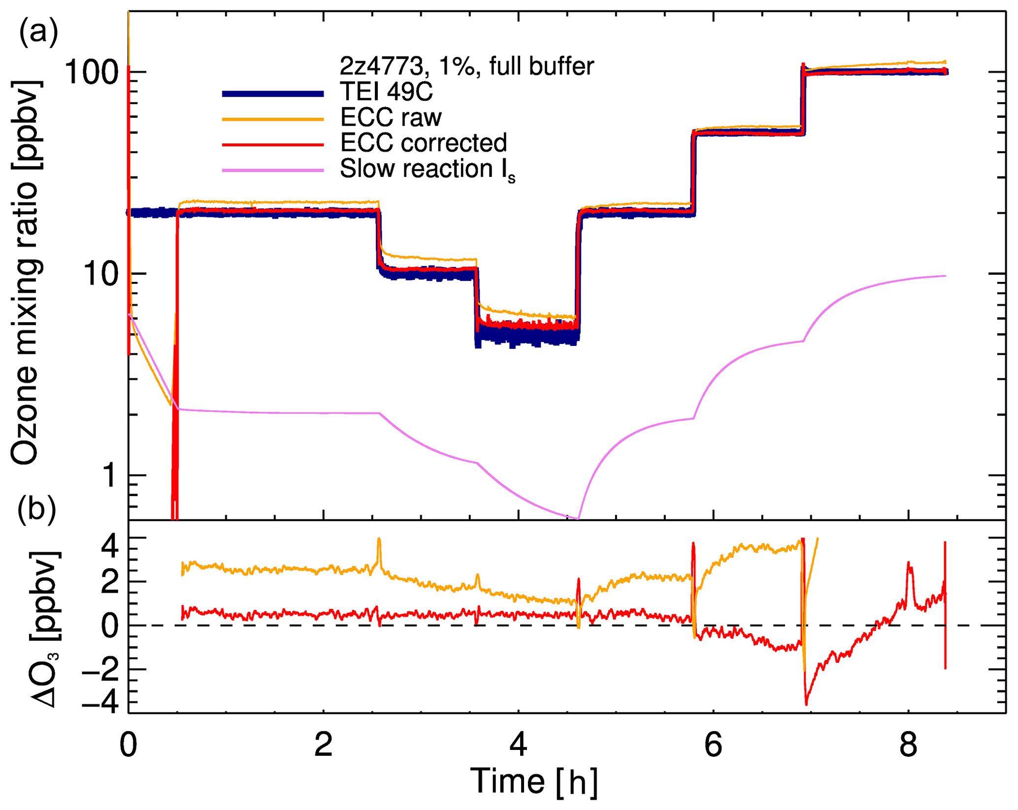
Figure 1 Top: ozone mixing ratio generated by the TEI 49C ozone calibrator (blue) and measured by the ECC (original processing in orange, time-response-corrected in red). The contribution of the slow reaction is shown in purple. Bottom: difference of raw (orange) and corrected (red) ECC measurements from TEI 49C ozone concentration.

The classical processing of the ECC ozonesondes in Eqs. (1) and (2) assumes a constant background current; however, the contribution of the slow-reaction pathway to the measured cell current is anything but constant. This result shows that using a “constant background” is not valid, regardless of which value is chosen.

The difference between the corrected ECC mixing ratio and the TEI 49C ozone calibrator (Fig. 1b) is nearly constant, with a value of 0.53 ppb, covering the first four step changes over the series, and the pattern differs significantly from the time-dependent difference shown in Fig. 3 of VD2010. The behavior of the difference changes after about 5.5 h, most likely due to evaporation of sensing solution.

Figure 2 Response of three ECC sondes using three different solutions during two plateau changes. The color-coding is the same as in Fig. 1. The reference time is defined as the time when the TEI 49C drops below 59 ppb during the first change in plateaus.

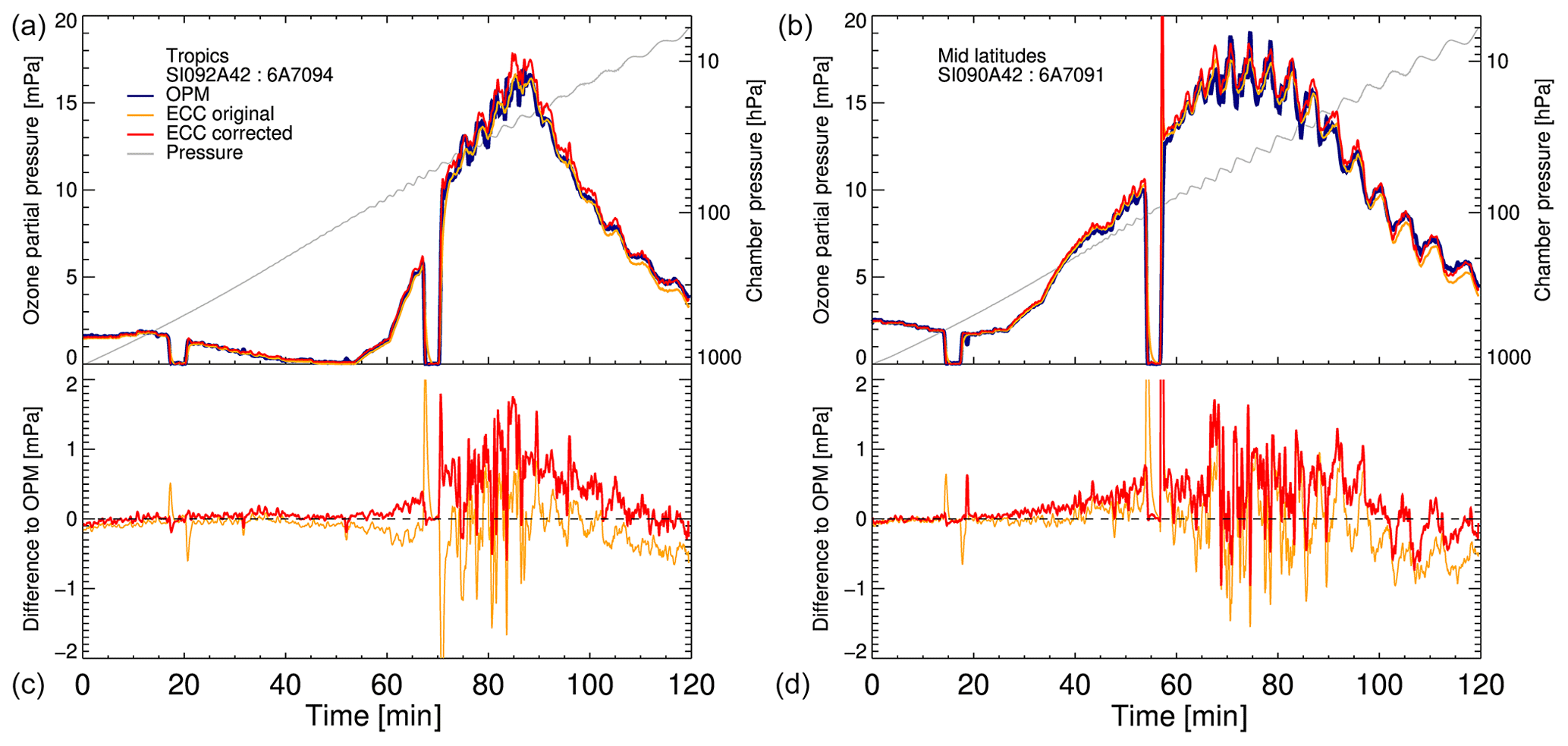
Figure 3 Reprocessing of JOSIE 2000 environmental simulation chamber ozonesonde data. (a) Tropical simulation, (b) midlatitude simulation. Blue lines in panels (a) and (b): ozone photometer measurements. Orange lines: originally processed ozonesonde measurements. Red lines: reprocessed ozonesonde measurements using the separation of slow- and fast-reaction contribution. Thin gray line: chamber pressure.

The effect of the time lag correction on the response of the ECC during the step changes is shown in Fig. 2. These experiments used two different 2Z series ECC sondes from EN-SCI and one 6A series ECC sonde from Science Pump Inc. as well as the three most common sensing solution recipes. While the originally processed measurements show the effect of response time lag, the corrected data show a response that is nearly indistinguishable from the drop in ozone generated by the TEI 49C. In particular, the small bias of the ECC remains almost constant across any step change.

The measurements show that the time response is nearly identical for these three sondes and sensing solutions, suggesting that this approach can be applied to the most commonly used sonde types and solutions. The time lag corrections for the six step changes shown in Fig. 2 are a representative subset of a total of 60 step changes in 25 different experiments. The correction approach may be applied to any of these instruments and solutions and could be used at operational stations to remove the effect of the slow reaction in existing time series. The small biases between the corrected ozone mixing ratio and the TEI 49C may in part be due to the accuracy of the TEI 49C calibrator and in part be specific to the individual sondes or sensing solutions used in these tests. The small observed differences may already be representative for the ECC model or sensing solution type; however, more work would be required to better explain these small differences.

3 Validation in independent laboratory experiments: JOSIE

The World Calibration Center for Ozone Sondes (WCCOS) at the Research Center Jülich has conducted a series of ozonesondes tests, comparing instruments operated by staff from different ozonesonde stations against a reference ozone photometer (OPM). The sondes were tested in the Environmental Simulation Chamber at Jülich, in which temperature, pressure, and ozone mixing ratio were regulated simultaneously to represent a midlatitude, a subtropical, and a tropical profile. Here, we use data from two ozonesondes tested during the Jülich OzoneSonde Intercomparison Experiment (JOSIE) in September 2000 (Smit et al., 2007).

The two sondes shown here used the 0.5 % KI, half-buffer solution and were originally processed with the pump efficiency correction of Komhyr (1986). We have reprocessed these measurements using the algorithms described above and summarized here: the slow-reaction contribution to the measured cell current was calculated iteratively using Eq. (6), a time constant of τ_s≈25 min, and a steady-state bias of 0.024 (2.4 %) based on VD2010. To initialize the calculation, we assumed that the “background” was measured 20 min before the start of the simulation and that the ozonesondes were measuring at the simulated surface value for that period. This calculated slow-reaction contribution was subtracted from the raw current instead of any “constant background” to provide the fast-reaction contribution (Eq. 7). To reduce noise in the subsequent time lag correction, the fast-reaction cell current was first smoothed using the Gaussian filter in Eq. (10). For correction of the time lag of the fast-reaction contribution (Eq. 9) we used the fast time constant reported for each JOSIE simulation, which had been measured prior to each simulation run (on the order of 20 s). In the calculation of the partial pressure and mixing ratio, we used the average pump efficiency correction reported by Johnson et al. (2002) for Science Pump 6A sondes.

Figure 3 shows simulations of a tropical and a midlatitude profile, including two periods each during which the ozone concentration in the chamber was switched to 0 to study the time response of the ozonesondes. The original ozonesonde measurements, the reprocessed data, and the differences to the OPM are shown. The pressure approximately followed a typical balloon ascent and is shown as well.

The reprocessing shows some interesting differences. The reprocessed tropical measurements between 55 and 100 min show on average about 5 % higher ozone than the reference, while the original data start with a low bias of about 10 % and then show agreement with the reference. During this time, the reprocessed data follow the OPM data slightly better than the originally uncorrected data. At the lowest pressures between 100 and 120 min, the reprocessed data do not fall off as rapidly as the originally processed data and show good agreement with the reference, while the originally processed data drop to a 10 % low bias. The different pump efficiency correction used in the reprocessing, which corrects the pump inefficiency at low pressures more strongly, contributes most to this difference, with a smaller contribution by the slow reaction.

In the simulated tropical profile, the reprocessed ECC ozone concentration in the simulated upper troposphere between 30 and 60 min is larger than the reference and much larger than the near-zero ozone concentrations reported by the original processing. However, since the true ozone concentration is very low, overall uncertainties and relative differences are large in this segment of the profile.

The reprocessed midlatitude simulation shows only small changes, except at the lowest pressures after about 100 min. Again, the reprocessed data do not drop off as quickly due to the different pump efficiency correction used with the reprocessed data.

Figure 4 shows the different cell current contributions of the original and reprocessed measurements. These data are shown on a logarithmic scale to highlight both slow- and fast-reaction contribution on the same plot. Most importantly, the slow-reaction contribution to the cell current may vary by almost a factor of 10 in both the tropical and the midlatitude simulation. This is in contrast to the assumption of a constant background in the original processing. The effect is most noticeable in the tropical simulation, where the background-corrected cell current is much smaller than the fast-reaction contribution to the cell current, leading to a strong underestimation of ozone. Past the ozone peak after around 60 to 90 min, the slow-reaction contribution is larger than the constant background assumption and slightly lowers the calculated ozone. However, since the total ozone concentration is large, the net effect is small. Near the end of the simulation, i.e., at the lowest pressure, the slow-reaction contributions become slightly larger and reduce the effect of the larger pump efficiency correction.

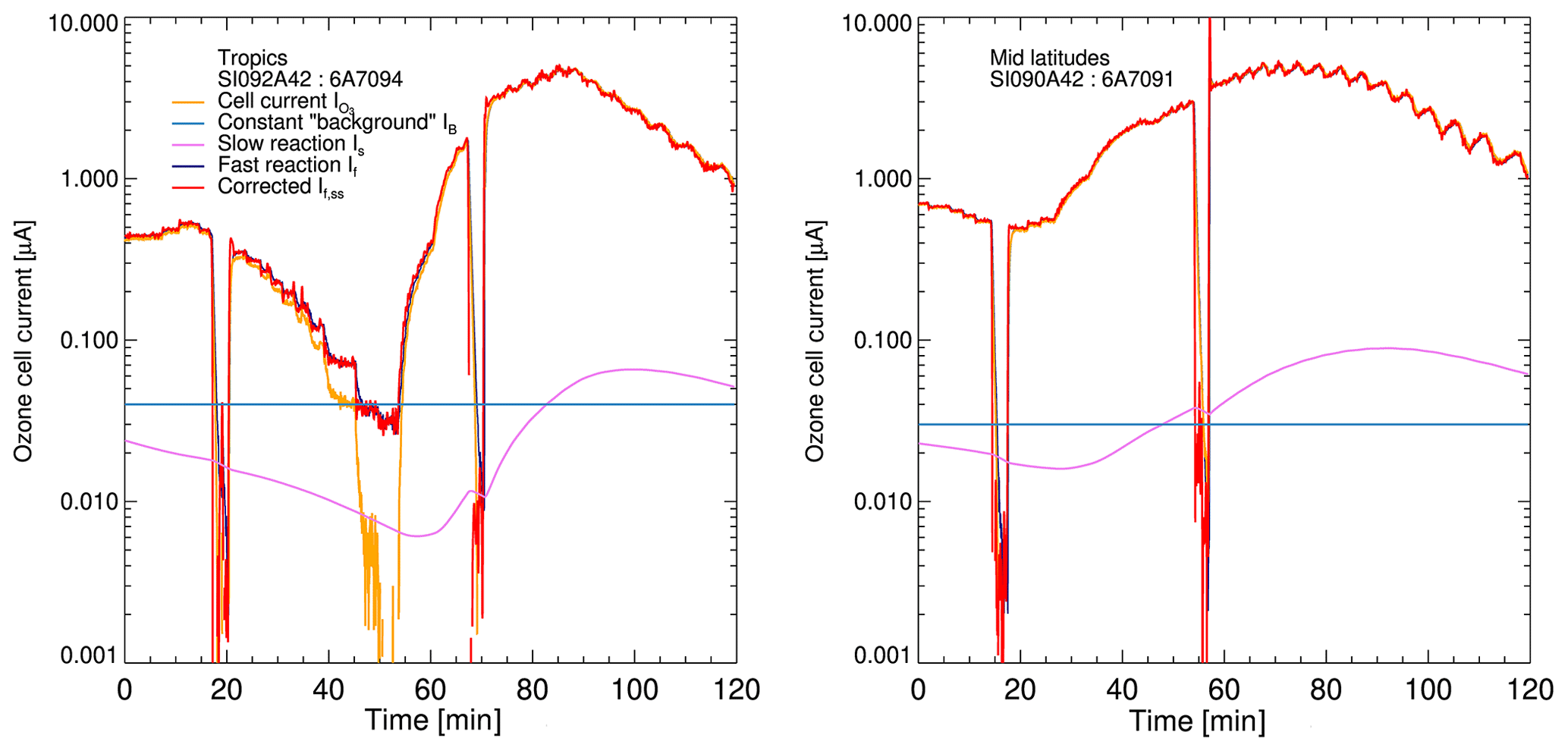
Figure 4 Cell current components of the tropical and midlatitude simulations shown in Fig. 3. Red lines: corrected cell current. Blue lines: fast-reaction contribution. Purple lines: slow-reaction contribution. Orange lines: originally measured cell current minus constant background. Light blue lines: constant background.

There is some uncertainty in the contribution of the slow-reaction pathway at the beginning of the simulation since the history of the ECC chemistry prior to the start of the data recording is not known. Changing the time when the background was measured (we assumed 20 min prior to the start of the simulation) has some influence on the slow-reaction contribution in the early phase of the simulation.

In both the tropical and midlatitude simulation, the reprocessed data show an improved response relative to the OPM reference compared to the originally processed data. The zero-ozone periods in both the tropical and midlatitude simulation after about 60 min are shown in Fig. 5 and demonstrate that the reprocessed ozone partial pressures closely follow those of the OPM. Results are very similar to the earlier zero-ozone periods at 15 min, confirming the improvement already seen in the lab measurements shown in Fig. 2.

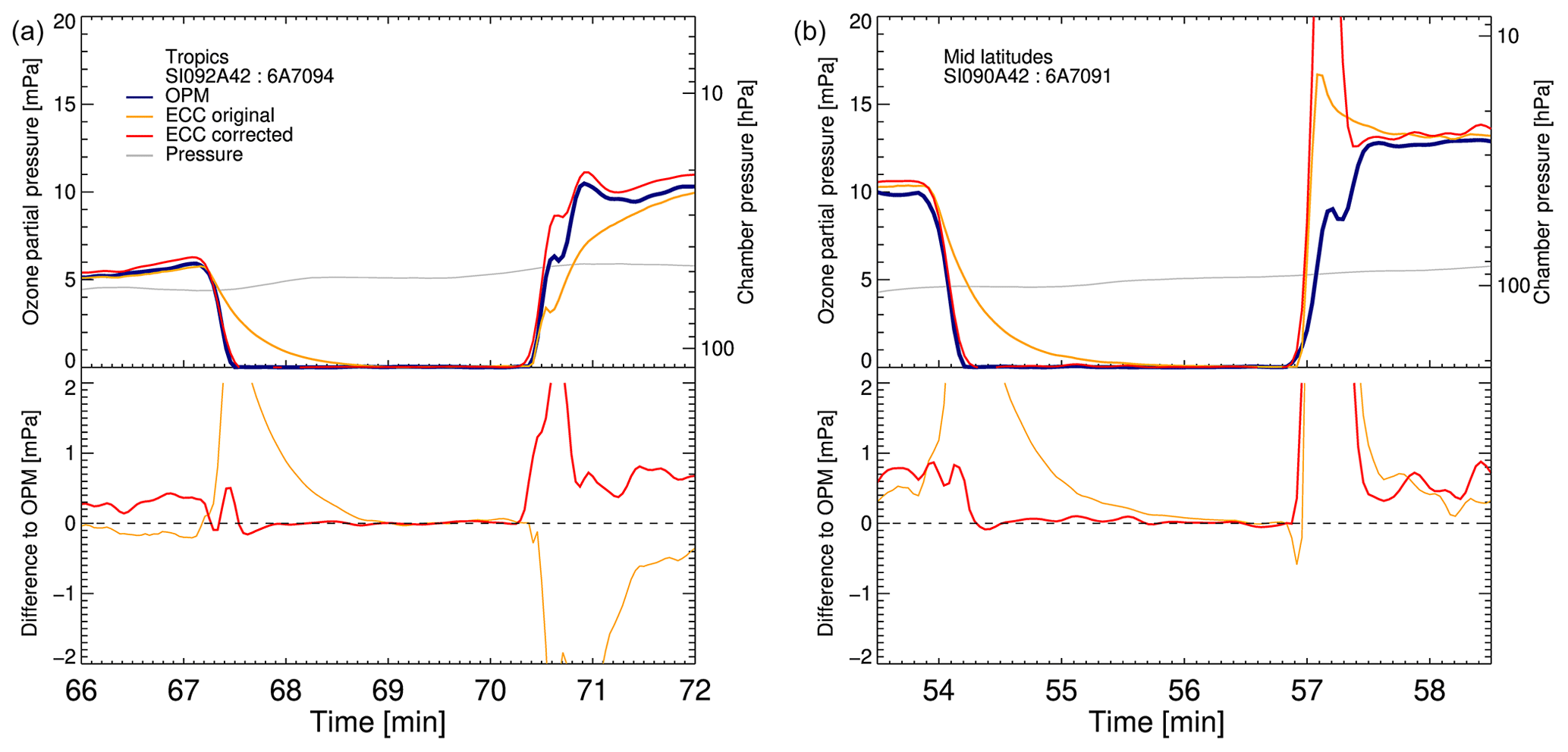
Figure 5 Same data as Fig. 3 showing the time response periods after about 1 h. (a) Tropical simulation, (b) midlatitude simulation. The differences are shown as absolute differences since the reference achieves zero ozone.

The integrated ozone amount in the reprocessed profiles is about 5 % larger than the OPM-integrated ozone for both the tropical and midlatitude simulation. This is slightly worse compared to the original processing, which had shown agreement with the OPM in the tropical simulation and a 3 % larger value for the midlatitude simulation. However, in the reprocessed simulations, the excess is almost constant throughout the entire profile, in contrast to compensation of excess and shortage in the original processing. These remaining biases indicate that not all sources of uncertainty have been captured yet; however, the improvement in consistency indicates a better understanding of the role played by the slow-reaction contribution.

The JOSIE 2017 campaign tested over 70 different sondes with a combination of sensing solutions and sonde manufacturers. Preliminary results are shown by Thompson et al. (2019), and these data are currently analyzed in more detail. Here, we applied the time response corrections to all simulations using the steady-state bias matching the respective sensing solution, the fast time response provided with each sonde run, and a slow time constant of 25 min. Furthermore, all simulations are processed using the pump efficiency corrections by Johnson et al. (2002). The average difference between the original and corrected sonde data and the OPM data is shown in Fig. 6. There are many details in this data set, which are smoothed out by the averaging and require a more detailed analysis, especially in the 12–20 km region, where the standard error is large. Nevertheless, we show that the structure in the difference profile is strongly reduced and that on average the ECC sondes agree with the OPM to well within 3 % throughout all pressures.

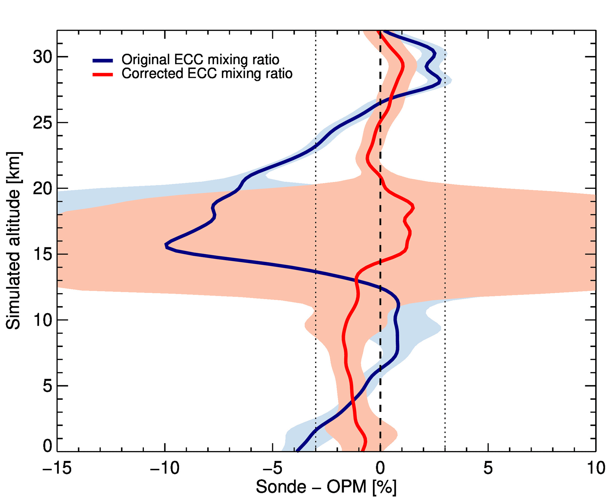
Figure 6 Comparison between ECC and OPM mixing ratio in 77 simulation experiments during JOSIE 2017. The originally reported difference is shown in blue; the difference calculated using the corrected data is shown in red. The shaded areas indicate the standard error. Dotted lines indicate ±3 %.

Differences due to sensing solution and manufacturer still require careful analysis; however, the much better agreement after applying the time response corrections shows that the time behavior of the ECC ozonesondes must be considered in the analysis of ECC ozonesonde data.

4 Application to atmospheric measurements

We processed the series of ozonesonde observations at Costa Rica using the algorithm introduced above to evaluate its impact on real-world observations. At that site, we have used the 1 % KI, 1/10th buffer solution since the beginning, with the exception of a short period when the 0.5 %, half-buffer solution was used. All soundings with the 1 % KI, 1/10th buffer solution used the pump efficiency correction by Johnson et al. (2002), while the sounding with the 0.5 %, half-buffer solution used the pump efficiency correction by Komhyr (1995). The steady-state bias for the 1 % KI, 1/10th solution was assumed to be 3.1 %, and that for the 0.5 %, half-buffer solution was assumed to be 2.4 % based on the measurements by VD2010. Figure 7 shows a profile measured at Heredia, Costa Rica, in 2010 and its reprocessed profile. The largest difference is in the upper troposphere and lowermost stratosphere with over 20 % larger reported ozone concentrations after reprocessing. At the top of the profile, the reprocessed ozone concentration is 5 % lower.

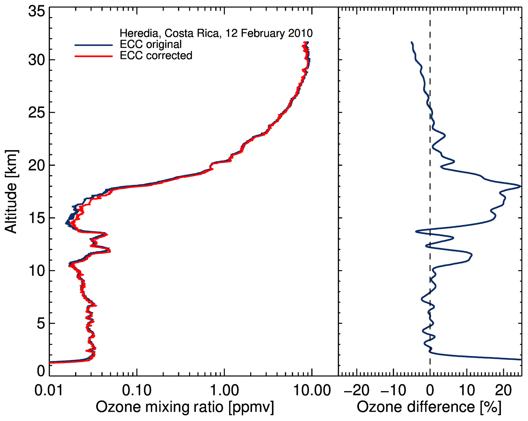
Figure 7 Ozone profile measured at Costa Rica. The original profile is shown in blue, the reprocessed profile in red. The right-hand profile shows the difference of the reprocessed profile minus the original profile.

The contribution of both the slow and the fast-reaction pathway is shown in Fig. 8. The constant background current used in the original processing is shown for reference. Up to about 23 km, the cell current contribution of the slow reaction is less than the original background current. In the stratosphere, the contribution of the slow-reaction pathway exceeds the original background current due to the slow buildup of secondary reaction products. This implies that the ozone profile has been slightly underestimated in the troposphere and slightly overestimated in the stratosphere.

Figure 8 Contribution of the fast-reaction path (red) and the slow-reaction path (purple) to the measured cell current. The constant background used in the original processing is shown for reference.

The effects of smoothing and correcting for time lag are shown in Fig. 9, where we show a close-up of the profile shown in Fig. 7. This particular sounding exhibits two significant peaks between 11 and 14 km. The originally analyzed profile is shown in blue. The first processing step (orange) removes the contribution of the slow-reaction pathway, followed by the Gaussian smoothing (purple) and finally the time-lag-corrected profile (red) on the right of the set of profiles. The difference between constant background subtraction and removing the slow-reaction component is evident in the agreement between the original and corrected profile at 10 km and a difference of about 15  % at 15 km.

Figure 9 Tropospheric detail of the ozone profile shown in Fig. 7.

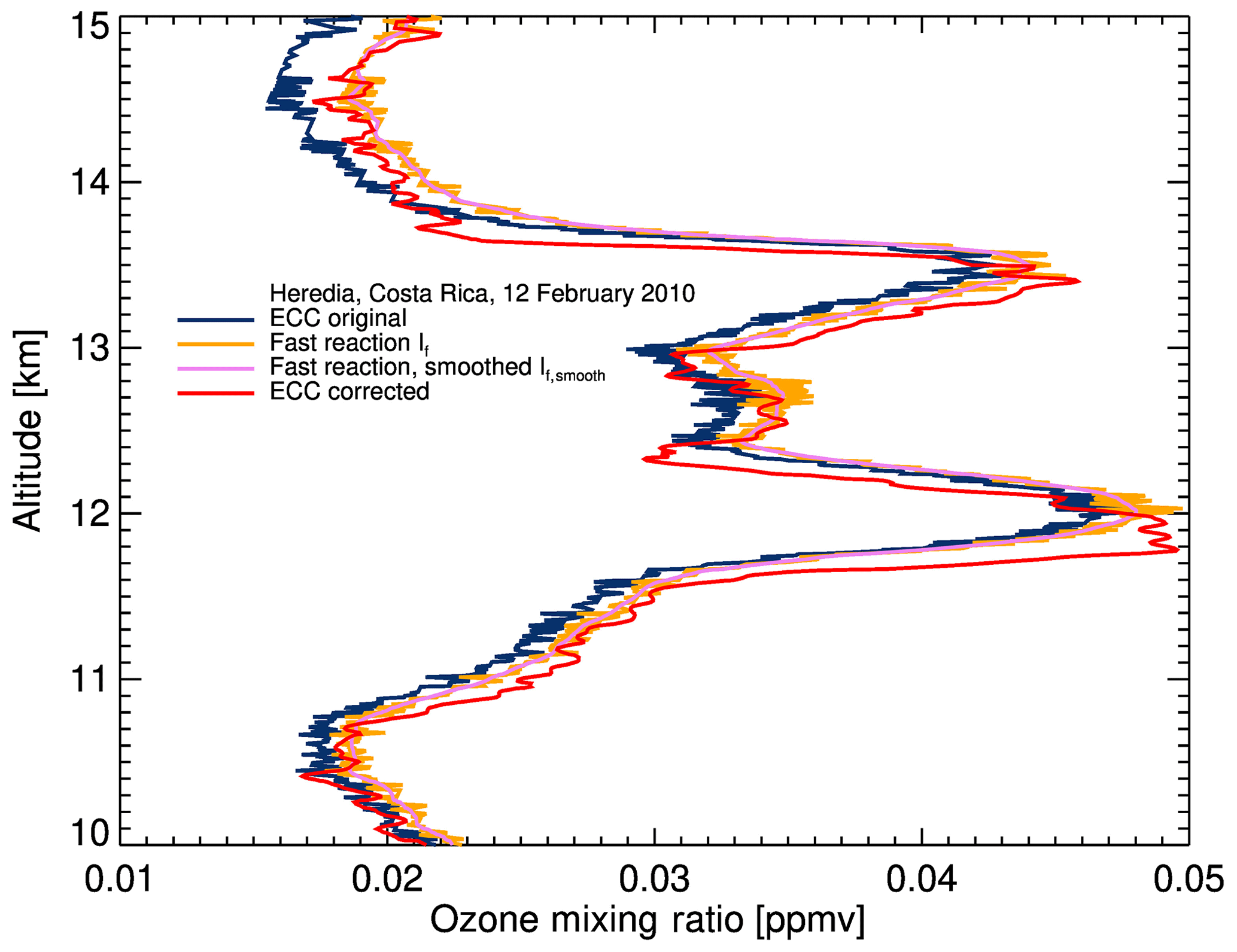
The time lag correction enhances both peaks by about 5 % and places them at a lower altitude than the uncorrected measurements by about 100 to 150 m. This amplification of features depends on the vertical gradient (see Eq. 9). In this example, the lower peak at 12 km is amplified stronger than the upper peak at 13.3 km because of its steeper gradient at a nearly identical rise rate of the balloon.

The noise amplitude of the time-lag-corrected data is comparable to that of the original data, but its spectral characteristics are different as a result of the smoothing algorithm. Therefore, scientific analyses should be based on layer averages since individual data points are heavily influenced by the noise characteristics of the smoothed data.

The behavior of the same ozone profile at and shortly after launch is shown in Fig. 10. The gradient of ozone above the surface layer is strongly enhanced by the time lag correction and appears even stronger in the corrected data than in the uncorrected data. (Note that in the laboratory experiments shown above, even stronger gradients are well represented after the corrections have been applied.) Furthermore, the measured ozone mixing ratio at launch depends on the history of the ECC prior to launch and therefore the operational procedures prior to launch. In Fig. 10, we show two profiles with different assumptions on the prelaunch history of the ECC. The purple trace assumes that the 5 µA ozone conditioning was stopped 40 min prior to launch and that the ECC was then exposed to zero-ozone air for 10 min, when it reached a preparation cell current reading of 0.05 µA. After that, it is assumed that the sonde was moved to the launch site and continued measuring until launch. The orange trace assumes that an ozone destruction filter was used between the 5 µA ozone conditioning and 5 min prior to launch. The difference between both cases is about 10 % at launch and decays after launch. The time between ozone conditioning and launch as well as the time prior to launch during which the ECC was exposed to ambient ozone is highly variable. As a result, the surface reading of operational ECC sondes at launch contains significant uncertainties, which decay within the first couple of kilometers as the ozone concentration above the surface increases and the influence of the operational procedures decreases.

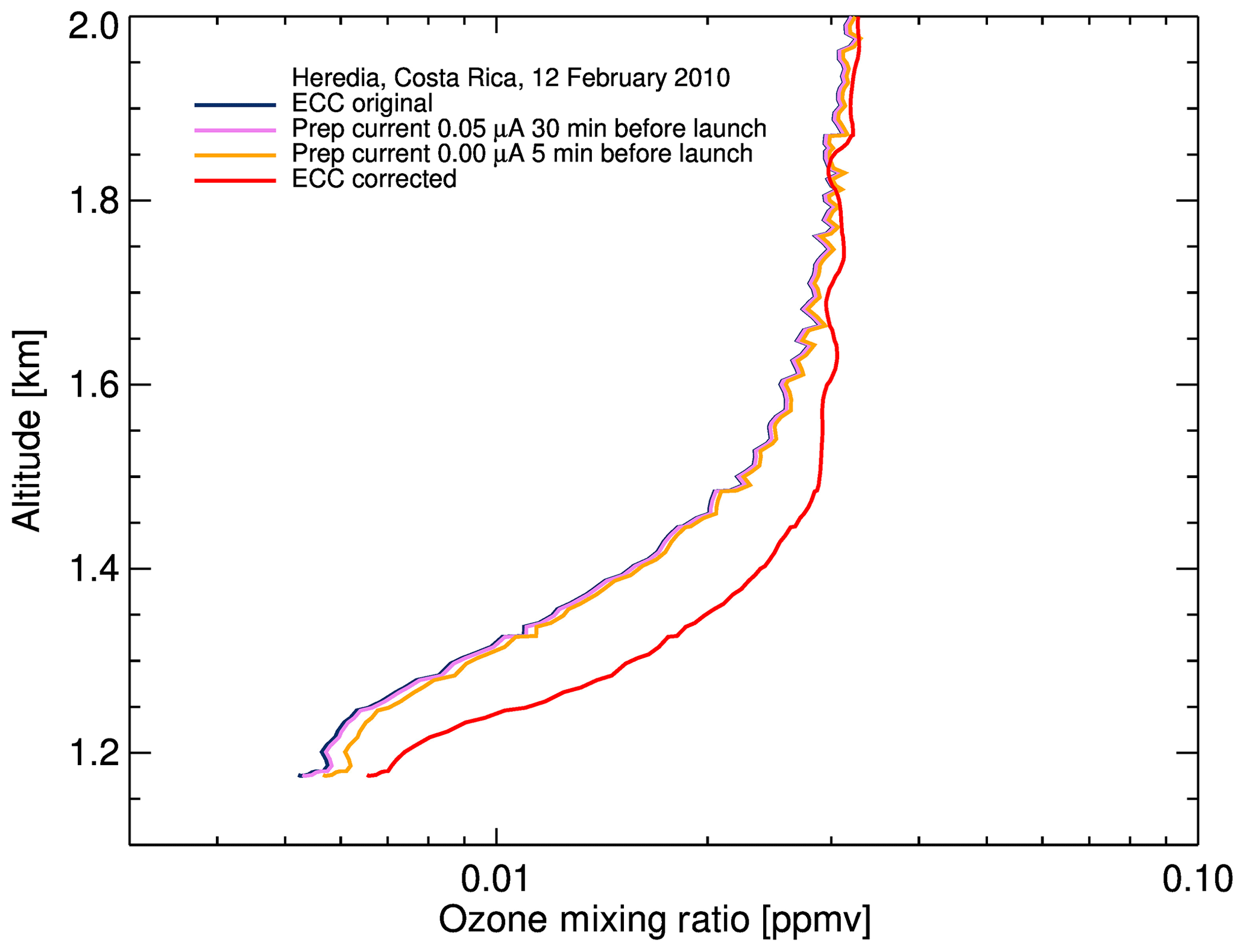
Figure 10 Boundary layer detail of the ozone profile shown in Fig. 7. The two different assumptions for the preparation current prior to launch have only been used for the slow-reaction path without applying a time lag correction for the fast-reaction path.

Newton et al. (2016) reported ozonesonde measurements from the western Pacific, where, due to failure of their sonde preparation equipment, a number of sondes were launched with very high background currents, which had to be corrected by an ad hoc hybrid background correction. We believe that this problem could be addressed using Eq. (6) and an appropriate choice for the slow-reaction contribution at the surface.

We have applied the correction algorithm to 577 ozonesondes launched at Costa Rica, which allows us to evaluate its impact statistically. The median difference between the corrected and originally reported ozone profiles is shown in Fig. 11. Here, we show the influence of only removing the slow-reaction contribution and of removing the slow-reaction contribution and applying the time lag correction.

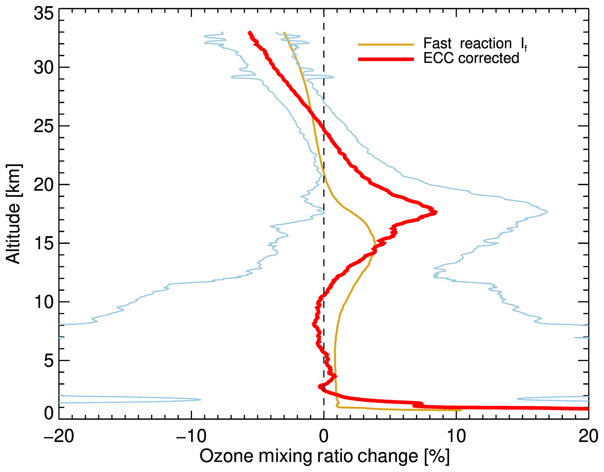
Figure 11 Median difference between corrected and originally reported ozone mixing ratio for 577 ozonesondes launched at Costa Rica. Thin orange line: fast-reaction contribution only. Thick red line: complete correction algorithm including time lag correction. The thin blue lines: 1 standard deviation around the complete correction algorithm.

Three features of the complete correction of removing the slow-reaction contribution and applying the time lag correction can be highlighted.

1. The surface layer readings are significantly increased with the new correction algorithm. However, the surface reading itself has a larger uncertainty than the rest of the profile. This effect disappears approximately 1–1.5 km above the surface.

2. The ozone mixing ratio in the upper troposphere and lower stratosphere between 10 and 25 km is larger as a result of these corrections, with the largest correction at the tropical tropopause. This increase is due to both processing steps, i.e., the smaller contribution of the slow reaction compared to the constant background current processing and the time lag correction. In fact, at the tropopause, at about 17 km, the change is mostly due to the time lag correction and less to the smaller slow-reaction contribution. The overall increase in this region is due to the mean shape of the tropical-ozone partial-pressure profile, which has its maximum around 25 km.

3. The ozone mixing ratio near the top of the profile decreases on average by about 5 %, which is in about equal parts due to the removal of the larger slow-reaction contribution and the time lag correction. The influence of the time lag correction is again due to the climatological shape of the tropical-ozone profile above the mean ozone partial-pressure maximum. This change improves agreement with simultaneous Microwave Limb Sounder (MLS) observations, which are lower than the Costa Rica sondes for much of the record (Stauffer et al., 2020).

Interestingly, there is very little change in the middle troposphere between about 3 and 10 km, where the different removal of the slow-reaction contribution compared to the constant background current is compensated by the time lag correction. This may be typical for tropical profiles but not necessarily for mid- and high-latitude profiles.

VD2010 had suggested using constant steady-state bias correction and a fixed small constant background current offset without consideration of the temporal response in processing of ozonesondes. The results shown here indicate that the time response of both the fast and slow reaction must be considered and may have equal contributions to the overall deviations from the simple ECC equation. A simple bias correction as suggested by VD2010 is not sufficient.

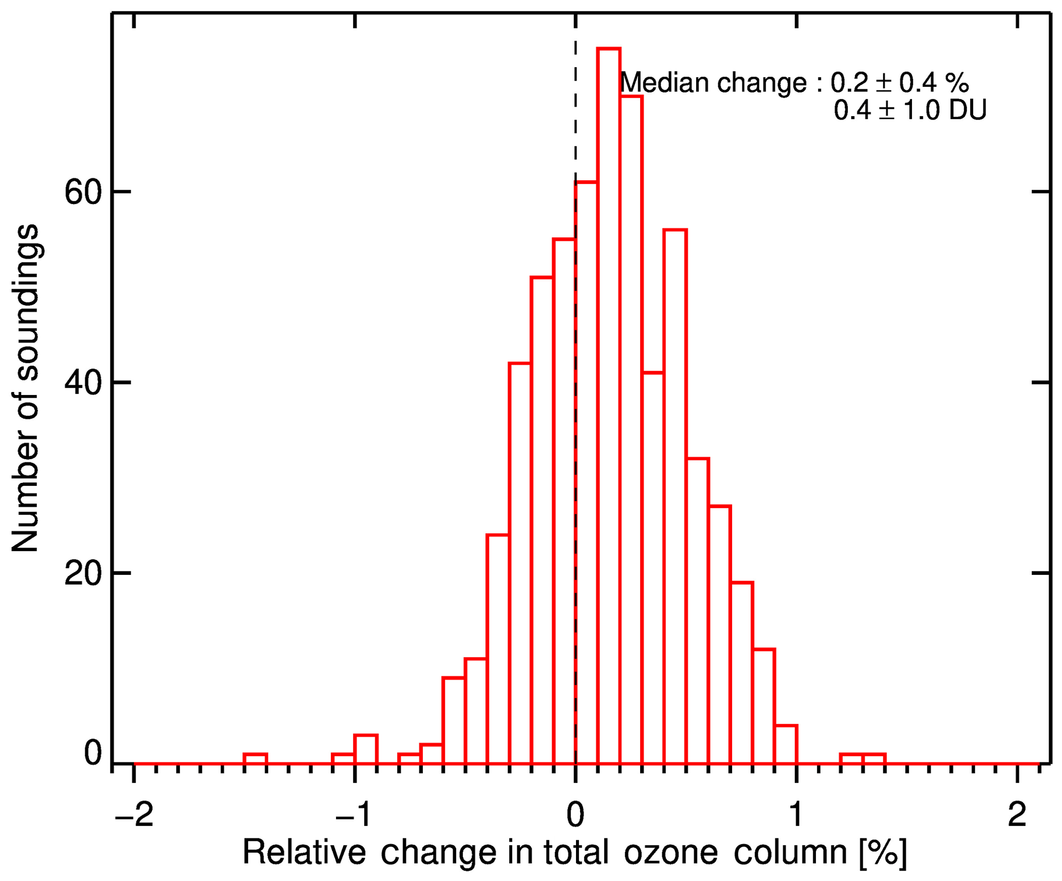
Figure 11 indicates that the areas of increased and decreased ozone mixing ratio are approximately equal. For the calculation of the total ozone column, these areas may cancel, and the influence on the total ozone column is likely small. Figure 12 shows a histogram of the change in total ozone column for all ozone profiles at Costa Rica and demonstrates that there is almost no change at all. The median change is 0.4±1.0 DU. Therefore, even though the profile structure is changed, comparisons with observations measuring total ozone column would not be affected much by these new processing algorithms, at least for sites such as Costa Rica.

Figure 12 Change in the total ozone column due to the correction algorithms.

We also applied the correction algorithms described above to 28 ozone profiles obtained during CEPEX, which had already been reprocessed by VD2010 to study the impact of the background current on ozone measurements in the upper tropical tropopause. VD2010 argued for a different treatment of the background current using a steady-state correction approach, in which a modified background depended on the instantaneously measured cell current. In contrast, here we explicitly consider the temporal behavior of the slow and the fast correction pathways separately. Furthermore, we use the pump efficiency correction by Johnson et al. (2002) instead of the original pump efficiency correction by Komhyr (1986). During CEPEX, the original 1 % KI, full-buffer solution was used; therefore, we use the steady-state bias of 9 % in Eq. (6) based on the measurements by VD2010.

Figure 13 shows the results explicitly considering temporal characteristics of the slow- and fast-reaction pathways. Panel a shows the originally processed and the reprocessed CEPEX data. Similar to VD2010, the most significant effect is in the upper troposphere, which eliminates all of the near-zero ozone observations. Panel b shows the contribution of the slow reaction in comparison to the original constant background current of 0.065 µA and the modified background used by VD2010. The slow-reaction contribution is similar to the modified background in VD2010 in the upper troposphere but smaller in the middle and lower troposphere and in the stratosphere, which is due to the slow buildup of the slow-reaction pathway with exposure to ozone. There is a significant spread in the slow-reaction contribution near the ceiling of the profile, which is in part also due to the significant variation in the balloon ascent rate during that campaign, giving some sondes more or less time to build up the contribution of the slow-reaction pathway. A simple scaling of the modified background as used by VD2010 overestimates that contribution and slightly underestimates the measured ozone in the stratosphere.

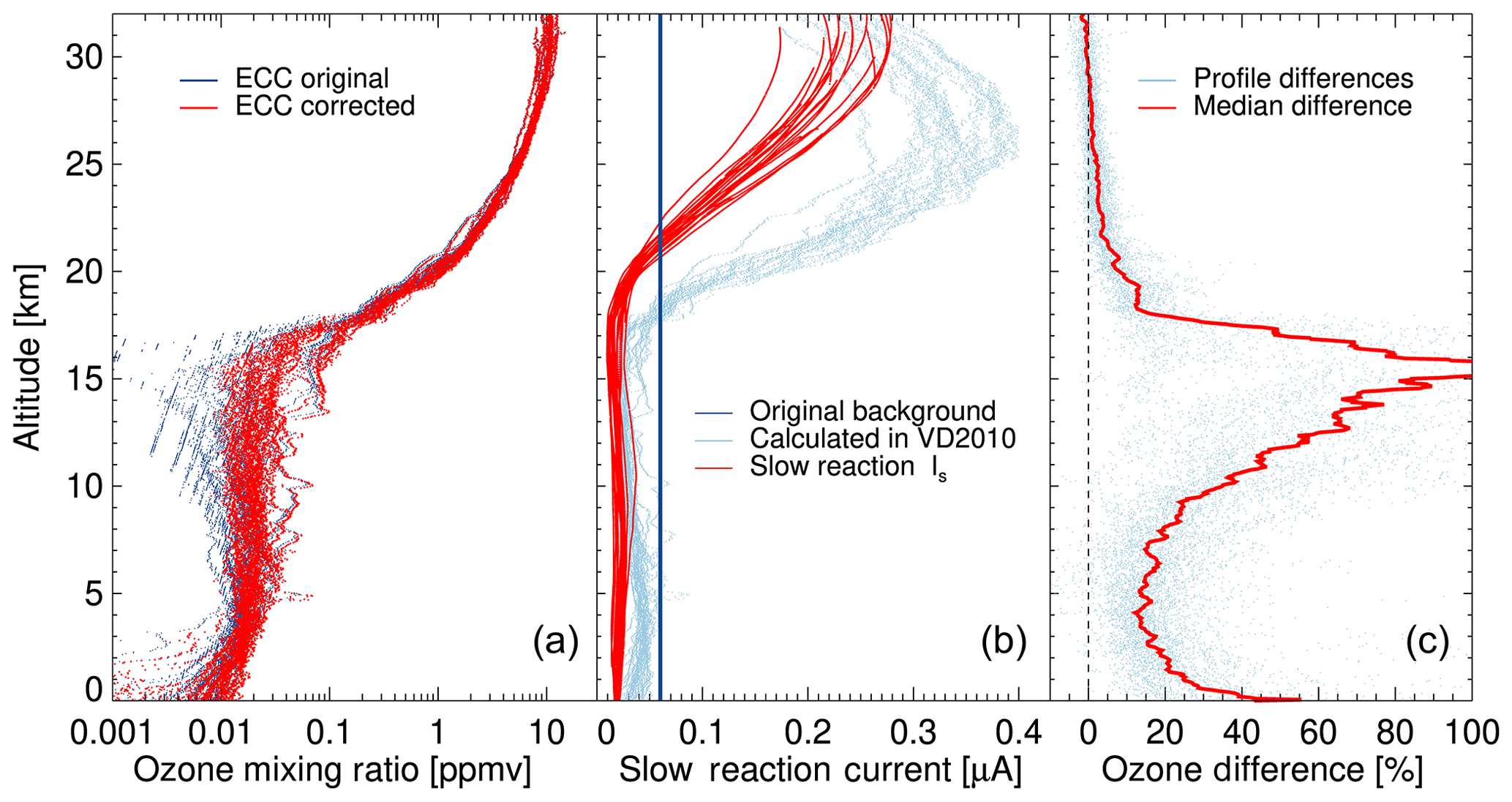
Figure 13 (a) Original and reprocessed CEPEX ozonesonde profiles. (b) Original constant background, reprocessed background following VD2010, and slow-reaction contribution. (c) Difference between reprocessed and original ozonesonde profiles.

The relative difference of the reprocessed and the original data is shown in panel c of Fig. 13. Similar to VD2010, the largest relative change is in the upper troposphere; however, the less obvious but more important result is that there is virtual agreement between the reprocessed and the original data near the ceiling despite using the stronger pump efficiency correction by Johnson et al. (2002). The mean total ozone column for the CEPEX data set changes by about 7 DU or 3 %. The increases in the upper troposphere, where the change in the pump efficiency correction is insignificant, contributes the majority of this change in the column.

In the reprocessed data, the excess cell current of the full-buffer solution is explicitly considered by removing the contribution of the slow-reaction pathway. This approach no longer requires the compensation of errors when using the weaker pump efficiency corrections by Komhyr (1986) and Komhyr et al. (1995), which compensate the excess cell current of the stronger-buffer solutions. Our approach allows processing of soundings with a proper pump efficiency correction and without the need to match the pump efficiency correction to the sensing solution.

The lowest part of the troposphere also shows a significant increase in the reported ozone after the reprocessing. However, this increase depends on the not-well-recorded use of the ozone destruction filter prior to launch. Here, we assumed that the slow-reaction contribution has decayed to 0.02 µA 5 min prior to launch based on scanning the available prelaunch data. However, there may be a significant uncertainty in this assumption.

5 Discussion

Processing ECC ozone data with an explicit calculation of the slow-reaction path and a time lag correction for the fast-reaction path requires knowledge about three coefficients: the slow-reaction time constant, the steady-state bias, and the fast-reaction time constant. In addition, an assumption about the partitioning of the measured cell current between slow- and fast-reaction pathway at the start of the data series is needed; however, this assumption mostly influences the calculated ozone mixing ratio in the boundary layer.

For the slow-reaction pathway, VD2010 reported values of 24 min for the 1 % KI, full-buffer solution and 28 min for the 1 % KI, 1/10th buffer solution, which is comparable to what has been reported by other studies (e.g., Davies et al., 2000). However, the exact value is not well known, and no level of confidence has been determined.

The steady-state bias depends on the sensing solution and has been reported by VD2010 and a number of other studies (e.g., Johnson et al., 2002; Smit et al., 2007). The measured values vary considerably, which is, in part, due to the laboratory setup and data analysis. Furthermore, the steady-state bias may change during a sounding as water evaporates from the solutions, increasing the concentration of its ingredients. A dependence of the steady-state bias on the temperature of the solutions may also be possible and has not been well studied.

A fast-reaction time constant is typically measured during the preparation of the ECC sonde and has been used in the analyses above. Komhyr and Harris (1971) and Komhyr et al. (1995) report a dependence of the fast-reaction time constant on temperature, solution volume, and pressure. During JOSIE (Smit et al., 2007), measurements of faster time constants after the completion of simulation runs were attributed to the evaporation of solutions. Therefore, the time constant measured during the preparation of ECC ozonesondes may not exactly represent the time response during a sounding.

To evaluate the uncertainty of the algorithm depending on the uncertainty of these coefficients, we repeat the correction of the ozone profiles at Costa Rica while independently varying the coefficients used in the correction. The slow-reaction time constant is varied by a factor of 2 from 12 to 50 min. The fast-reaction time constant is varied by a factor of 1.5 from 0.66⋅τ to 1.5⋅τ, where τ is the originally measured fast-reaction time constant. The steady-state bias reported by VD2010 for the 1 % KI, 1/10th buffer solution is varied by a factor of 2 from 1.5 % to 6 %. We estimate that these intervals cover a range, which includes the true value with a 95 % probability (2 sigma).

Figure 14 shows the contributions to the uncertainty of the corrections of the ozonesonde record at Costa Rica shown in Fig. 11. The single most important source of uncertainty in the corrections is the uncertainty of the steady-state bias, which dominates the uncertainty budget in the free troposphere and the middle stratosphere. Only in the lowermost stratosphere and the surface layer, the regions of the strongest gradients in the ozone profile, is the uncertainty of the fast-reaction time constant the dominant contribution. These regions are also the regions experiencing the largest correction. The uncertainty of the slow-reaction time constant is secondary throughout the entire profile.

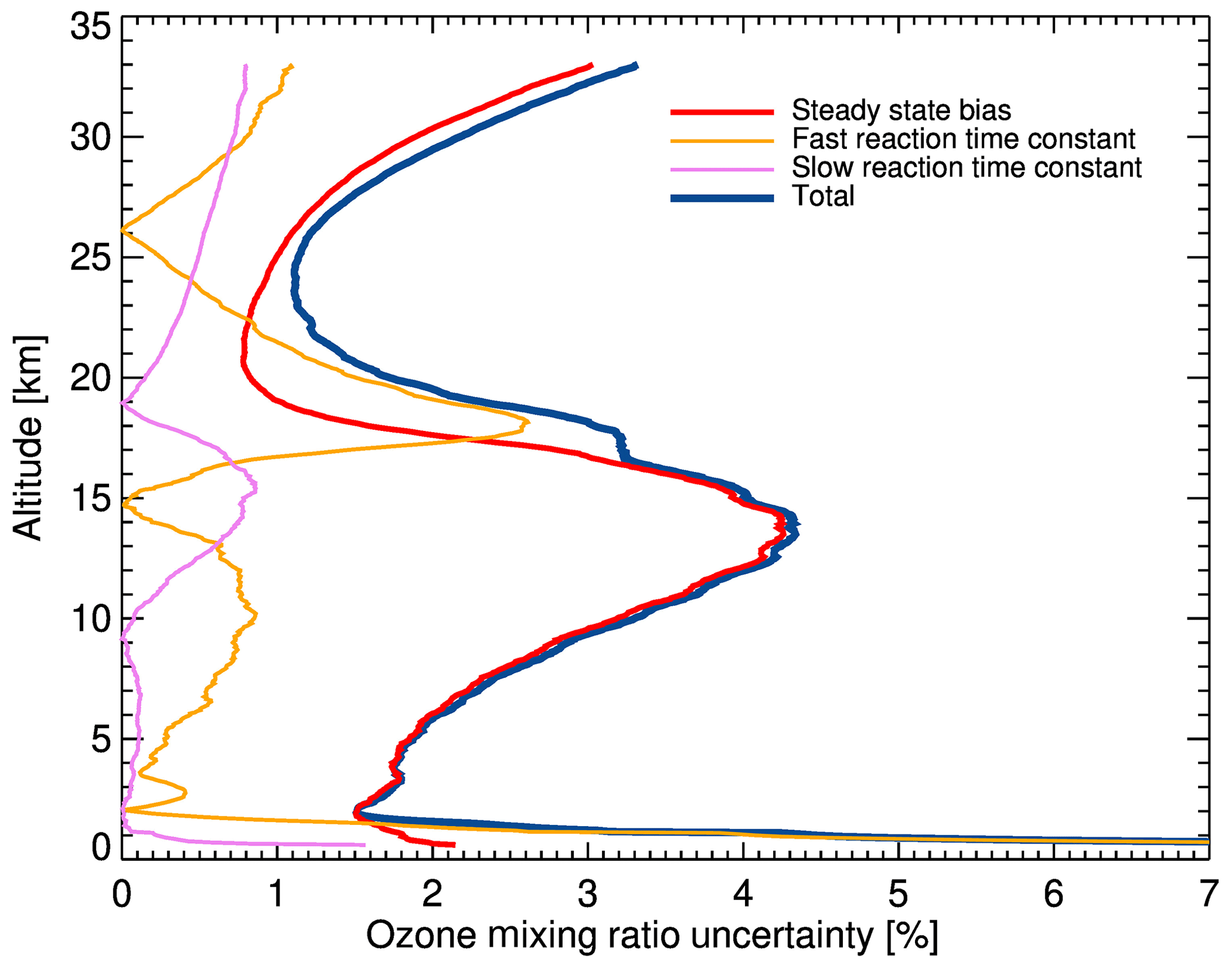
Figure 14 Contributions to the total uncertainty introduced by the correction shown in Fig. 11.

Therefore, further studies, such as a detailed analysis of all JOSIE simulations, may focus on a better quantification of the steady-state bias of the different sensing solution recipes.

The uncertainties discussed here describe the mean removal of systematic biases due to the time response of ECCs for the entire data set and help quantify the uncertainty of ozonesonde profiles in the validation of remote-sensing observations. Estimating the uncertainty of the correction of individual profiles, which depends strongly on the structure of each profile, requires a more detailed analysis based on that profile structure.

The corrections and uncertainties discussed here apply only to the time response model described above. Other effects, such as response differences of sondes from different manufacturers and pump-related effects, are not captured by the processes described here. However, the corrections for time response of the ECC need to be considered in properly quantifying other processes influencing the accuracy of ECC ozonesondes.

6 Summary

Two reaction pathways occur in an ECC ozonesonde, each of which generate electrons: the well-understood reaction between ozone and iodide, which generates two electrons per ozone molecule, and a secondary slow reaction, which generates additional electrons but which is not well understood. Here we consider explicitly the time constants of both reaction pathways to derive the ozone partial pressure. The contribution of the slower secondary reactions to the measured cell current is calculated separately and subtracted from the measured cell current. The remaining fast-reaction component is then smoothed using a Gaussian filter and corrected for its lag in response. The resulting corrected fast-reaction cell current, which is attributed to the ozone–iodide reaction, is finally used to calculate the ozone partial pressure. This approach overcomes the question whether there is a constant or a decaying background current and replaces it with the calculation of the contribution of the slow secondary reaction.

The algorithm considers the steady-state bias of the different sensing solution recipes, allowing processing of any sensing solution independent of the pump efficiency correction. Selecting weaker and inappropriate pump efficiency correction factors to compensate for side reactions in more strongly buffered solutions is no longer required to produce profiles in good agreement with validating measurements (e.g., JOSIE chamber experiments; Ozone Monitoring Instrument-integrated – OMI-integrated – columns; etc.).

The cell current measured during preparation while ozone-free air is pumped through the cell, which has been called the background current, should rather be called “postpreparation current” and should not be subtracted as a background current from the cell current during flight. This measurement is an indication of the proper functioning of the sonde and serves as an acceptance criterion for the instrument and the preparation procedure as long as a certain threshold is not exceeded. It is not a property of the sonde that remains constant throughout operation.

The time lag correction of the fast-reaction pathway enhances vertical features and removes a systematic bias, which is introduced in regions of strong gradients due to the relatively slow response relative to the balloon ascent rate, i.e., a low bias in the region below the ozone peak and a high bias in the region above the ozone peak.

An initial value for the slow cell current contribution is required during the analysis of the profile data. This value may be derived from experience, it may be measured using a high-quality filter prior to launch, or it may be set to 0. The contribution of this choice decays with the slow time constant and mostly influences the uncertainty of the ozone concentration in the boundary layer. It has no influence on the ozone measurements above the middle troposphere, in particular in the tropical upper troposphere, where erroneous background current values have led to very large uncertainties (e.g., VD2010; Witte et al., 2018). Specific requirements for the operating procedures prior to launch may help reduce the uncertainty in the boundary layer and will be included in the revised standard operating procedures.

The net effect of this process on the total ozone column derived from ECC sonde launches at Costa Rica is 0. Therefore, this correction does not affect the comparison with remote-sensing instrumentation measuring the total ozone column, at least for the 1 % KI, 1/10th buffer solution and using the correct pump efficiency correction measured by Johnson et al. (2002); however, it will affect comparisons with other profiling instruments.

Reprocessing the CEPEX data using this method achieves a similar result in the upper troposphere as VD2010 but improves the ozone calculation in the stratosphere since it allows replacing the old incorrect pump efficiency correction by Komhyr (1986) with the better pump efficiency correction by Johnson et al. (2002).

More work is required to properly quantify the steady-state bias of the different sensing solutions based on high-quality laboratory measurements. The theoretical understanding of both chemical pathways needs to be improved, which may lead to a further refinement of the approach demonstrated here. However, it is clear that including the reaction dynamics in the processing already removes some systematic biases, which have previously only been addressed through ad hoc methods.

Other processes affecting the uncertainty budget of ECC ozonesondes such as the different conversion efficiency of sondes from different manufacturers, the uncertainty of the pump efficiency, or a possible temperature dependence of the chemical processes have not been considered here. These effects need to be studied separately; however, they do require the recognition that the time dependence of the chemistry plays an important role in calculating the concentration of ozone under realistic (i.e., nonsteady-state) conditions.