the Creative Commons Attribution 4.0 License.
the Creative Commons Attribution 4.0 License.
 | 26 Oct 2020
Wuhan MST radar: technical features and validation of wind observations
Lei Qiao
Shaodong Zhang
Qi Yao
Wanlin Gong
Mingkun Su
Feilong Chen
Erxiao Liu
Weifan Zhang
Huangyuan Zeng
Xuesi Cai
Huina Song
Huan Zhang
Liangliang Zhang
The Wuhan mesosphere–stratosphere–troposphere (MST) radar is a 53.8 MHz monostatic Doppler radar, located in Chongyang, Hubei Province, China, and has the capability to observe the dynamics of the mesosphere–stratosphere–troposphere region in the subtropical latitudes. The radar system has an antenna array of 576 Yagi antennas, and the maximum peak power is 172 kW. The Wuhan MST radar is efficient and cost-effective and employs more simplified and more flexible architecture. It includes 24 big transmitter–receiver (TR) modules, and the row or column data port of each big TR module connects 24 small TR modules via the corresponding row or column feeding network. Each antenna is driven by a small TR module with peak output power of 300 W. The arrangement of the antenna field, the functions of the timing signals, the structure of the TR modules, and the clutter suppression procedure are described in detail in this paper. We compared the MST radar observation results with other instruments and related models in the whole MST region for validation. Firstly, we made a comparison of the horizontal winds in the troposphere and low stratosphere observed by the Wuhan MST radar with the radiosonde on 22 May 2016, as well as with the ERA-Interim data sets (2016 and 2017) in the long term. Then, we made a comparison of the observed horizontal winds in the mesosphere with the meteor radar and the Horizontal Wind Model 14 (HWM-14) model in the same way. In general, good agreements can be obtained, and this indicates that the Wuhan MST is an effective tool to measure the three-dimensional wind fields of the MST region.
- Article
(9992 KB) - Full-text XML
-
Supplement
(786 KB) - BibTeX
- EndNote


Mesosphere–stratosphere–troposphere (MST) radars have been used for studying the dynamics of the lower and middle atmosphere up to 100 km altitude for several decades (Hocking, 2011), since Woodman and Guillen observed radar echoes from the stratospheric and mesospheric heights with the Jicamarca radar in the 1970s (Woodman and Guillen, 1974). In general, a large antenna array is employed by these MST radars to measure the weak echoes scattered by the turbulence (Green et al., 1979). Many MST radars have been developed worldwide by different countries and groups, and the MST community plays a significant role in technique sharing. According to the antenna array shape, the existing MST radars in the world can be divided into two types: the square array arranging the elements in a square gird and the circular array arranging the elements in a triangular grid. The MST radars using the square array mainly include the Jicamarca radar (Woodman and Guillen, 1974), the SOUSY radar (Schmidt et al., 1979), the Poker Flat radar (Balsley et al., 1980), the Esrange MST radar (Chilson et al., 1999), the Gadanki radar (Rao et al., 1995), the Chung-Li radar (Rottger et al., 1990; Chu and Yang, 2009), and the NERC MST radar (Vaughan, 2002; Hooper et al., 2013). The MST radars using the circular array include the MU radar (Fukao et al., 1985; Kawahigashi et al., 2017), the EAR radar (Fukao et al., 2003), the MAARSY radar (Latteck et al., 2012), and the PANSY radar (Sato et al., 2014).
In 2008, construction of the Wuhan MST radar and Beijing MST radar began with the support of the Meridian Project of China (Wang, 2010). We introduced the two MST radars of the Chinese Meridian Project in 2016 (Chen et al., 2016). This paper briefly introduced the antenna array of the Beijing and Wuhan MST radars and their preliminary observations. The two MST radars work more than 280 d every year, and their data can be freely accessed in the data center for the Meridian Project (https://data.meridianproject.ac.cn/, last access: 6 July 2019). Thus, the radar system and their data have gained extensive attention and we have received many letters inquiring about the details of the radio system, as well as the data format and reliability. Therefore, this article has been written in response to the demands of the readers and users who want to build a low-cost MST radar or apply the data of the MST radars of the Chinese Meridian Project. The paper presents more details of the Wuhan MST radar including some optimized circuits, as well as its recorded data.
The Wuhan MST radar is located in Chongyang, Hubei Province, China (29.5∘ N, 114.1∘ E). The location is far away from the bustling city so as to better avoid interference by radio noise. Considering this is China's first attempt to develop its own MST radar, the radar station has not been placed in an area in which construction would be difficult, such as equatorial low latitudes, polar regions, and plateaus. Chongyang is located in the central plain of China, which is an appropriate choice. As one of few MST radars in the midlatitudes, it can be one important member of the group of global MST radars. In addition to aiding scientific research goals, the Chongyang station serves as a students' training base for the practice of radar technologies and meteorological applications. The Wuhan MST radar was completed preliminarily in 2011. The system was upgraded in 2016, and the transmitter–receiver (TR) modules were updated for better stability and better detection capability. The facility has cost only about USD 1 million, which is far lower than the high cost of other MST radars. However, it provides an average power aperture product (PAP) of 3.2×10⁸ W m2. Considering the balance of system performance and project implementation, simpler and more flexible architectures are applied in the system.
The first aim of the present paper is to introduce the technical features of the Wuhan MST radar. In particular, the antenna field, the timing signal, the TR module, the digital receiver and the clutter suppression will be discussed in detail. The second aim of this paper is to present the recorded data and compare them with the wind fields recorded by other instruments and related models for validation.
2.1 General description
The Wuhan MST radar is arranged in a 24×24 matrix, which consists of 576 Yagi antennas, with a side length of 96 m. Each antenna is driven by an individual small TR module (300 W). According to the antenna radiation pattern, the beamwidth is 3.2∘. The shortest width of the subpulse is 1 µs to satisfy the requirement for a maximum range resolution of 150 m. The radar system allows very high flexibility of waveform parameters for different detection modes (low mode, middle mode, and high mode). The basic specifications of the Wuhan MST radar are in Table 1. The hardware of the Wuhan MST radar consists mainly of five subsystems: the antenna array, the TR module, the radar controller, the digital transceiver, and the signal processor. Figure 1 shows the schematic block diagram of the system.

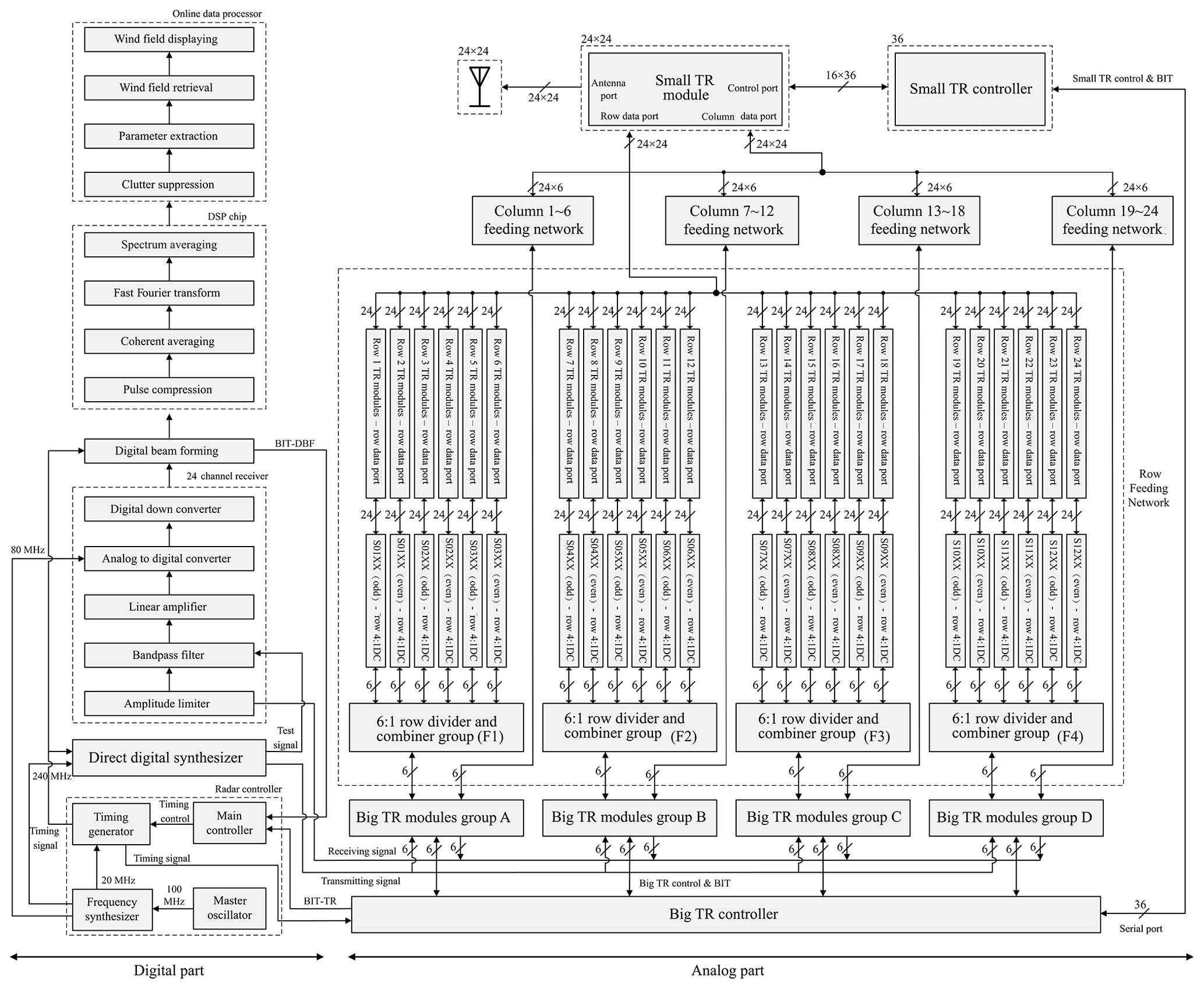
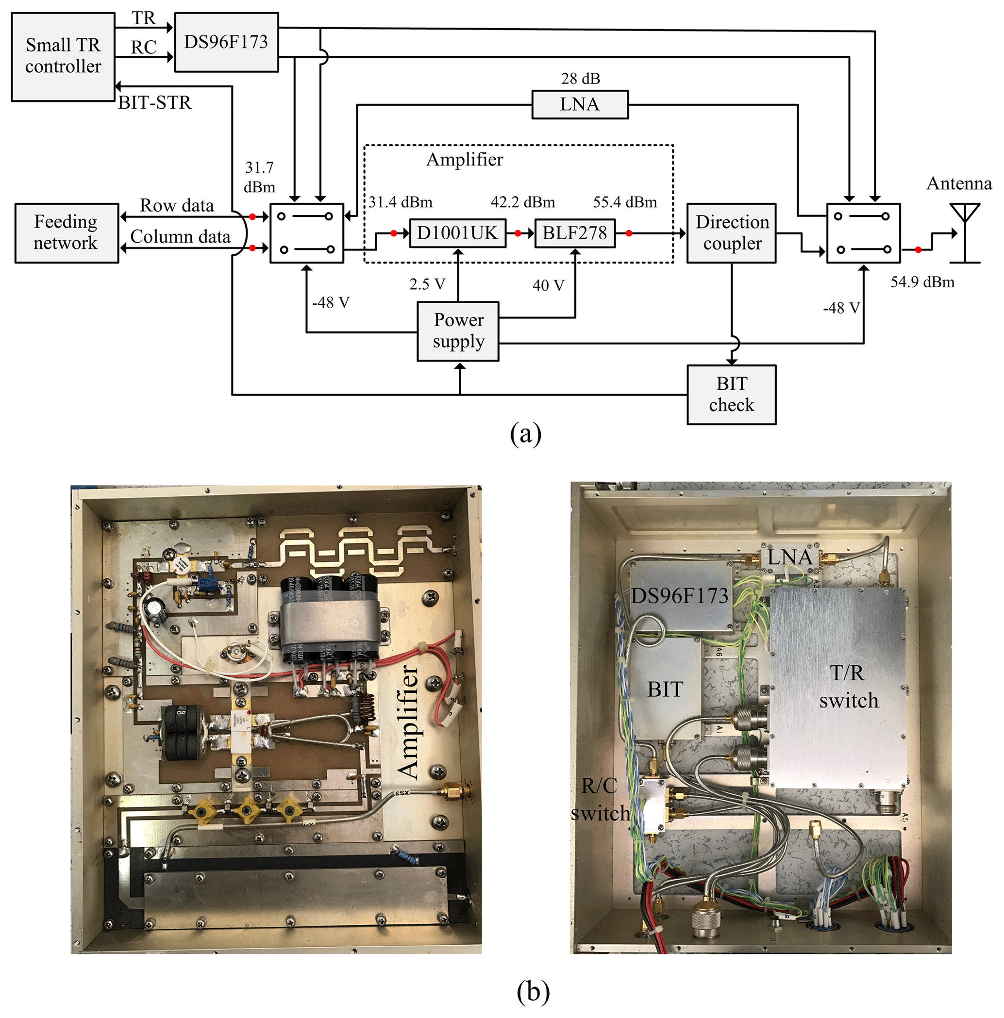
Figure 1Schematic block diagram of the Wuhan MST radar located in Wuhan, China. The small TR module controllers, the small TR modules, the feeding network, and the antenna array are installed in the antenna field. Other modules are installed in the observation house.
The signal scattered by “refractive-index irregularities” is received by the antenna array and then sent to the TR module by the feeding network. The TR module includes 24 big TR modules installed in the observation house and 576 small TR modules installed in the shelters. The big TR controller receives the timing signal from the timing generator in the radar controller by parallel port. The big TR controller converts the timing signal into multiplex signals to control the 24 big TR modules. At the same time, the BIT-TR signal is sent to the main controller to monitor the condition of the big TR module. The big TR controller also handles communication with 36 small TR module controllers over twisted-pair cabling, and each big TR module controller corresponds to 16 small TR modules. The row data port in the big TR module connects 24 small TR modules in a row of the antenna array via the row feeding network, while the column data port connects 24 small TR modules in a column via the column feeding network.
The radar controller consists of a master oscillator, a frequency synthesizer, a control timing generator, and a main controller. The master oscillator generates the reference clock of 100 MHz. Then, the frequency synthesizer generates the sampling clock of 80 MHz, the direct digital synthesizer (DDS) clock of 240 MHz, and the control reference clock of 20 MHz. Combined with the reference clock of 20 MHz and the commands from the main controller, the control timing generator generates various timing signals for radar control.
The digital transceiver consists of the DDS module and the 24-channel receiver. The DDS module is used to generate the binary-phase-coded continuous wave for transmitting and the test signal for channel calibration. The 24-channel receiver includes the amplitude limiter, the bandpass filter, the linear amplifier, the analog-to-digital converter (ADC), and the digital down converter (DDC). The amplitude and phase weight algorithm is realized in the digital beamforming (DBF) module.
The data processing implemented in the digital signal processing (DSP) chip involves pulse compression, coherent averaging, fast Fourier transform (FFT), and spectrum averaging. Then, the output of the DSP chip is transferred to the online data processor by a peripheral component interconnect (PCI) bus. The main functions of the online data processor are clutter suppression, parameter extraction, wind field retrieval, and wind field displaying. Eventually, the product data of the wind field in the troposphere, lower stratosphere, and mesosphere are produced.
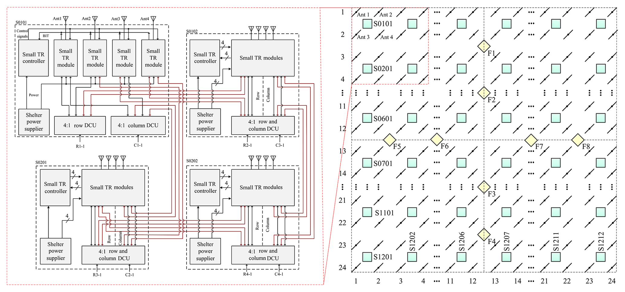
Figure 2Arrangement of the Wuhan MST radar antenna field and interconnections of four surrounding shelters.
2.2 Antenna field
Figure 2 shows the arrangement of the Wuhan MST radar antenna field. The Yagi antennas are arrayed on grids of squares with about 4 m sides, and this element spacing allows no grating-lobe beam scanning up to an angle of about 24∘ from zenith.
The voltage standing wave ratio (VSWR) of the antenna is less than 2.5.
As shown in the right part of Fig. 2, there are 144 shelters mounted at regular intervals, and each one consists of four small TR modules, a 4:1 row divider–combiner unit (DCU), a 4:1 column DCU, a power supplier, and a small TR controller. It should be pointed out that the 36 small TR controllers are located in the shelters of odd rows and columns. The eight yellow boxes, labeled F1–F8, represent the row feeding boxes (F1–F4) and the column feeding boxes (F5–F8). Each feeding box contains six 6:1 DCUs, and each one feeds four 4:1 DCUs in the shelters. The DCUs in the row and column feeding boxes are all fed by the big TR modules in the observation house, and the row or column drive state is switched by the control signal. The row/column data from the 24 big TR modules feeding the 6:1 row/column DCUs are labeled R1–R24/C1–C24.
As illustrated by the red box in the right part of Fig. 2, there are four shelters (S0101, S0102, S0201, S0202) and the surrounding antennas. The left part of Fig. 2 shows the interconnections of the shelters, and the lines of different shelters are red for easy review. In the shelter S0101, the row DCU is fed by R1-1, which represents the first divided signal of R1. The other four ports of the row DCU connect to the row data ports of the small TR module 1 and 2 in S0101 and S0102, respectively. Similarly, the column DCU is fed by C1-1 and the other four ports connect to the small TR module 1 and 3 in S0101 and S0201, respectively. By analogy, the row and column DCUs of the shelters S0102, S0201, and S0202 connect to proper data ports of the small TR modules. With this system configuration, the beam can be steered to the north–south direction in the row drive state and east–west direction in the column direction. The antennas are aligned in the northwest–southeast direction for a symmetrical radiation pattern. The beams are usually steered to five directions (vertical, north, south, east, west) with off-zenith angles of 15∘.
The feeding network of the Wuhan MST radar uses feeding cables of equal length. In this situation, the feeding cables of different channels have stable characteristics, which need no compensation. The big TR modules, the 6:1 dividers and combiners, the 4:1 dividers and combiners, and the antennas are connected via coaxial cable (−3 dB per 100 m). The feeding cables of the above modules are 100, 50, 10, and 7 m, respectively. Therefore, the feeding-line loss from the TR module in the observation house to the end antenna of the array is about 5 dB.
2.3 Timing signal
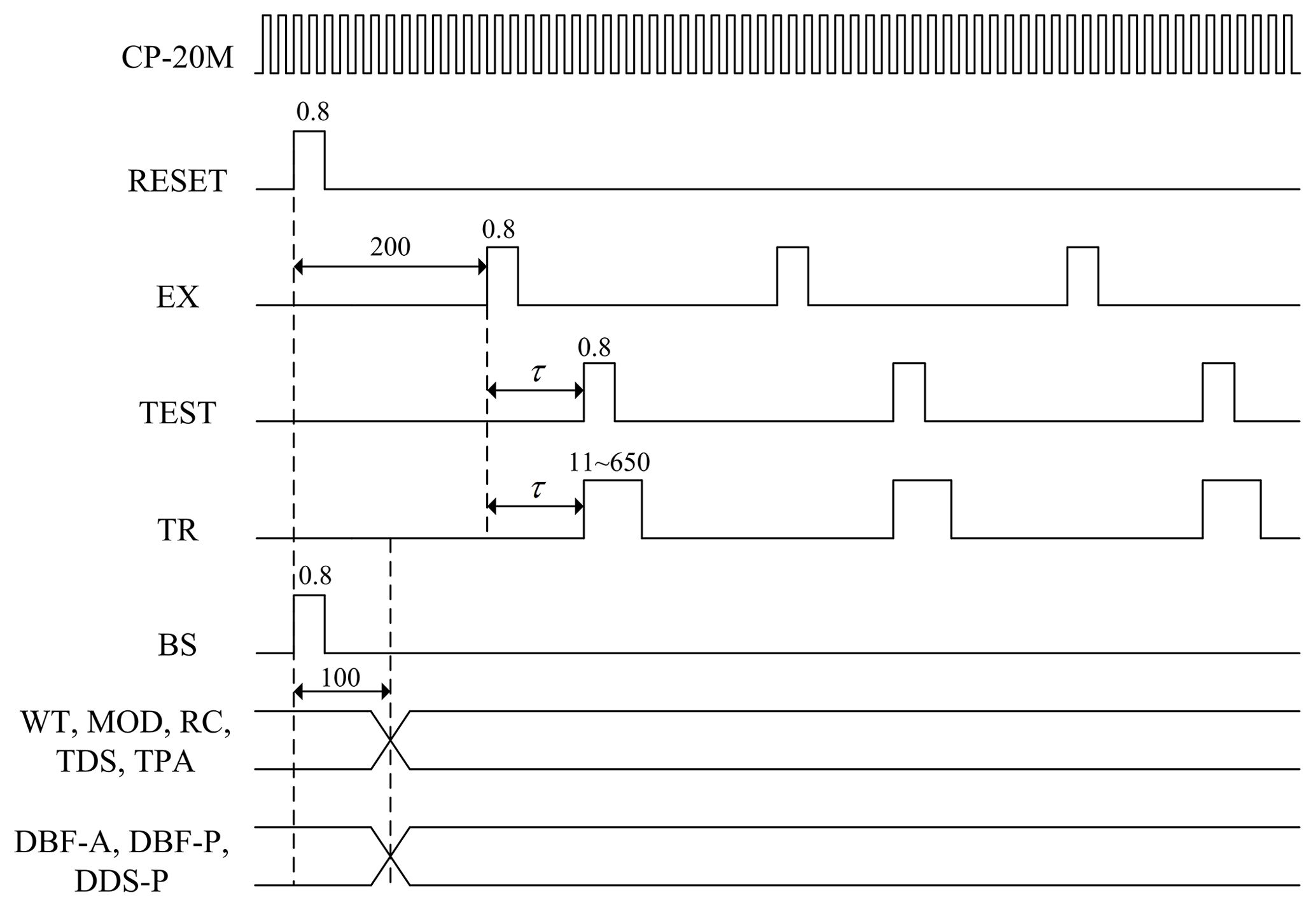
All timing signals for radar operation are generated by the timing generator in the radar controller. Figure 3 presents the timing diagram of the signals at the radar controller. They are generated from the reference clock signal of CP-20M. The RESET signal is used to activate the timing generator. The excitation (EX) signal is used to generate the pulse repetition period (PRP), and the value is different according to different detection modes. The EX signal is 200 µs later than the RESET signal. The sign τ is the delay of the TEST signal and the TR signal compared to the EX signal. The delay can be adjusted by software, and the range is from a half clock period ahead to a half clock period delay. The transmitted pulse width of the TR signal is from 11 to 650 µs, which is related to the compressed pulse width and the coding scheme. The beam switch (BS) signal controls the switching of the vertical beam and four oblique beams, and it is synchronized with the RESET signal.
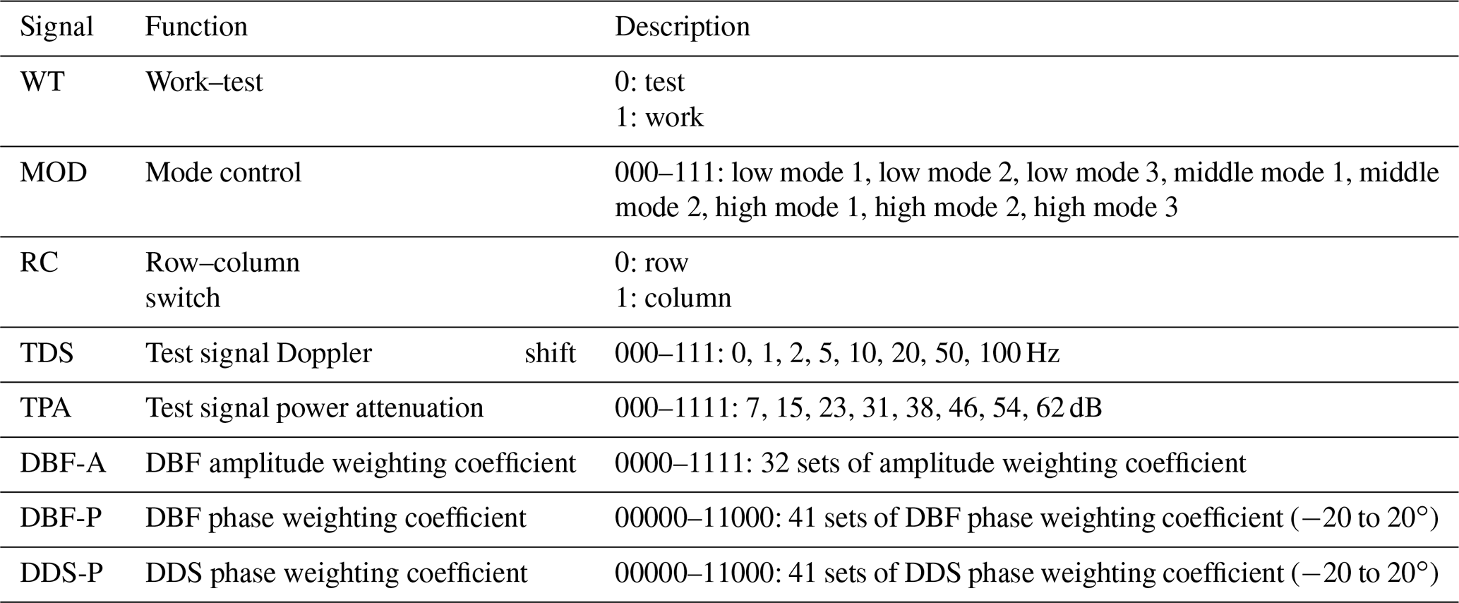
Besides the transmitting and receiving timing signals, the radar controller also generates the control signals for system control, which are shown in the last two lines of Fig. 3. It should be pointed out that the control signals are valid 100 µs after the RESET signal rising edge. The different control signals are listed in Table 2. The work–test (WT) signal causes the system to operate in work mode or test mode. The test mode is applied for digital receiver channel calibration. The mode control (MOD) signal is used to select the observation mode: low mode (troposphere), middle mode (stratosphere), and high mode (mesosphere). The low mode 1, middle mode 1, and high mode 1 are usually selected under normal operating conditions. The corresponding Doppler resolution and radar scanning time are 0.53 m s−1 and 5 min, respectively. The parameters of the other observation modes can be set flexibly for applications of high Doppler resolution. The row–column (RC) switch signal is used to control the RC switch in the small TR modules and big TR modules. The test signal Doppler shift (TDS) signal sets the test signal to establish different values of Doppler shift, which serves the digital channel calibration. The test signal power attenuation (TPA) signal controls the attenuation coefficient of the test signal so as to prevent damage to the digital receiver. The DBF amplitude weighting coefficient (DBF-A) signal and the DBF phase weighting coefficient (DBF-P) signal are used for beamforming in the DBF module. The DDS phase weighting coefficient (DDS-P) signal causes the DDS to generate beams of different zenith angles with a step size of 1∘, and the maximum angle is 20∘.
2.4 TR module
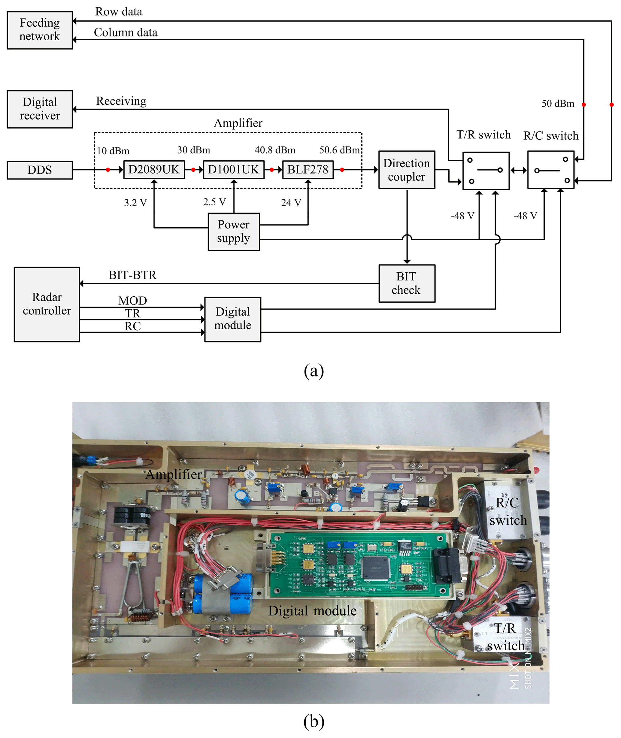
A block diagram and photograph of the big TR module are shown in Fig. 4. The big TR module amplifies the DDS output (53.8 MHz) supplied from the digital transceiver module and feeds it to the feeding network. This module consists of a three-stage amplifier with a gain of 40.6 dB. D2089UK and D1001UK, whose drain–source voltages are 3.2 and 2.5 V, respectively, are employed in the first and second power amplifier stages. They are metal gate radio-frequency (RF) silicon field effect transistors (FETs) with different power outputs. The DDS output (10 dBm) is amplified to 30 dBm in the first stage, while the first stage output is amplified to 40.8 dBm in the second stage. The push–pull-power metal oxide semiconductor (MOS) transistor BLF278, whose drain–source voltage is 24 V, is employed in the final stage with a gain of 9.8 dB. A built-in test (BIT) technique is adopted to detect the VSWR and power information of the amplifier output (50.6 dBm) via a directional coupler. The information is used to not only monitor the status of the big TR module but also avoid damage to the amplifier. The insertion loss of the TR switch and RC switch in the big TR module is about 0.3 dB. Therefore, the total output becomes 50 dBm.
The control signals transferred from the big TR controller are transformed over twisted-pair cabling for better transmission ability. The TR signal (differential signal) is converted into a single-ended signal by the differential converter, and then it controls the RC switch to realize transformation of the row or column. The differential receiver chip DS96F173 is used as the differential converter, which allows operating at high speed while minimizing power consumption. The TR signal controls the TR switch to receive the signal from the row or column data port or to transmit the amplifier output to the row or column data port. The MOD signal is transferred to the digital module so as to generate timing signals to control the TR switch and RC switch for different observation modes. The recovery time of the two switches is less than 5 µs, which reaches the allowable level. The power supply provides −48 V for the two switches. It should be pointed out that the differential converter is involved in the digital module, as shown in Fig. 4b.
A block diagram and photograph of the small TR module are shown in Fig. 5. The small TR module consists of various submodules: an amplifier, a TR switch, an RC switch, a BIT module, and a differential receiver. Each row or column signal is divided equally into 24 signals in the feeding network. Considering the attenuation of the dividers and cables (100 m cable −3 dB; 1:6 divider −7.78 dB; 50 m cable −1.5 dB; 1:4 divider −6.02 dB), the transmitting signal from the big TR module is reduced to 31.7 dBm. Then the signal is transmitted through a low-power RC switch with 0.3 dB insertion loss. A two-stage amplifier in the small TR module amplified the signal from 31.4 up to 55.4 dBm, and the drain–source voltage of BLF278 is 40 V with a gain of 13.2 dB. Then, a bandpass filter centered on 53.8 MHz is provided for spurious emission suppression. The TR switch in the small TR module has an insertion loss of about 0.5 dB and provides an isolation of 60 dB. Ultimately, the output of the small TR module is about 300 W, and the signal is fed to the Yagi antenna via a 7 m coaxial cable. The low-noise amplifier (LNA) in the receiving channel is a 53.8 MHz tuned amplifier with a gain of 28 dB and a bandwidth of 1 MHz.
The two switches embedded in the small TR module allow the controller to select the proper signaling pathway, and they are both controlled by two control signals from the small TR radar controller. The small TR module is the most easily damaged part in the system. Therefore, it needs to be repaired every year. As shown in Fig. 5b, the small TR module adopts the modular design, which is convenient for maintenance.
2.5 Digital transceiver
The digital-up-converter (DUC) chip AD9957 is used in the DDS module, which has a 1 Gsps internal clock speed with an 18 bit IQ data path and 14 bit digital-to-analog converter (DAC). The 16 or 32 bit complementary code with different pulse widths (1, 4, and 8 µs) is generated by the DDS module, as well as by the test signal. The passive calibration algorithm is used for amplitude and phase calibration of the 24 channels in the receiver. The test signal can be set with different values of Doppler shift and is divided into 24 channel signals by the divider. The intrinsic amplitude and phase differences among channels can be extracted by comparing the output of each channel. Then, the amplitude and phase calibration factors are stored in the register. Through correction, the receiver has an amplitude consistency of −0.5 to 0.5 dB and a phase consistency of −2 to 2∘ after calibration.
In the receiver, the signal firstly goes through the amplitude limiter for protection of the receiver, then the linear amplifier with 50 dB gain, and the bandpass with a center frequency of 53.8 MHz and bandwidth of 1 MHz. Then, the signal is sampled by the LTC2208 with an 80 Msps clock rate. It is an ADC with 16 bit resolution, a maximum of 130 Msps, and a 100 dB spurious free dynamic range (SFDR). By directly bandpass sampling, the received signal is aliased to 26.2 MHz. The DDC unit is integrated into the FPGA, which is made up of the numerically controlled oscillator (NCO), the cascade integrator comb (CIC) filter, and the finite impulse response (FIR) filter. In general, the frequency output of the NCO is 26.2 MHz, the bandwidth of the FIR filter is 1 MHz, and the total decimation value is 80. Eventually, the in-phase (I) component and quadrature-phase (Q) component with 1 MHz are transformed to the digital beamforming module for further processing.
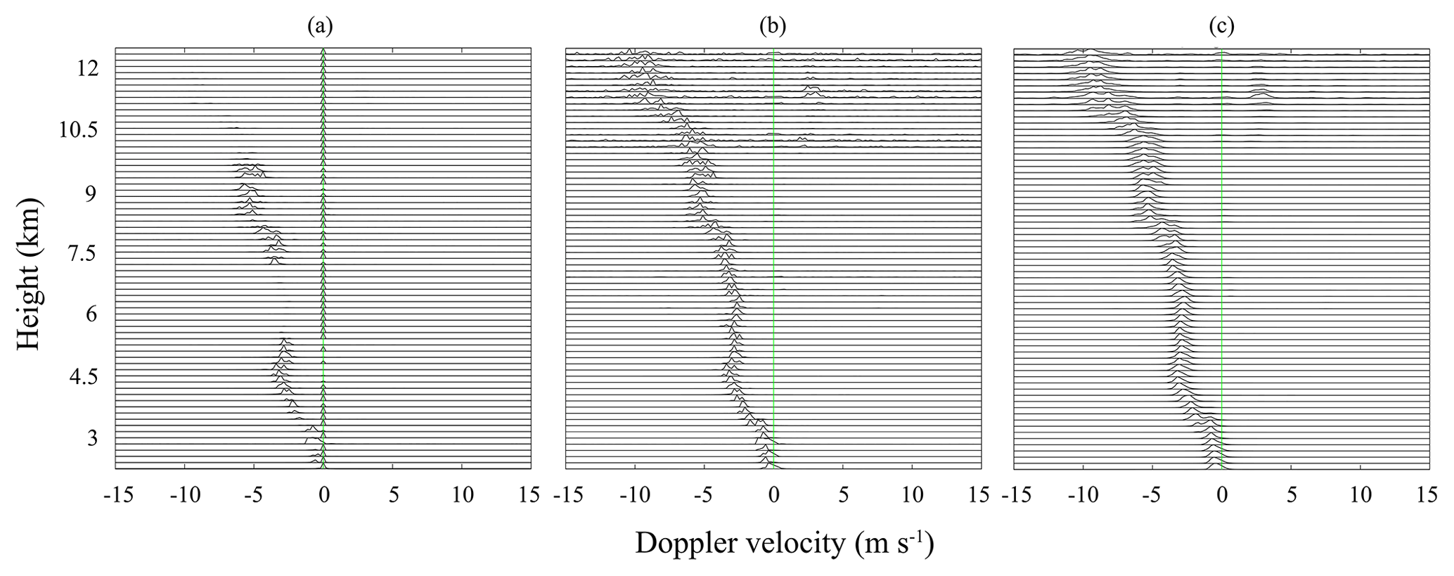
Figure 6Comparison of the original (a), ground-clutter-suppressed (b), and filtered (c) Doppler spectrum.
2.6 Clutter suppression
The clutter suppression is carried out with an online data processor. Kumar et al. (2019) identified the turbulence echo in the multipeaked very high frequency (VHF) radar spectra during precipitation, and here we mainly aimed to investigate ground clutter and high frequency interference during fair weather. Ground clutter from surrounding mountains, trees, and buildings can severely degrade parameter estimates of turbulence (Schmidt et al., 1979). This is because the weak echoes from the clear air are easily contaminated by the larger amplitude of the ground clutter. From the perspective of radar infrastructure, the construction of a fence is an effective method to isolate ground clutter, e.g. the 10 m height MU radar fence for ground clutter prevention (Rao et al., 2003). A fence is also constructed for the Wuhan MST radar, but there is still some ground clutter in the echoes. Therefore, ground clutter suppression is an essential step for signal processing. The ground clutter echoes have a narrow central peak near zero frequency with small temporal changes and are weakened with increasing altitude.
Figure 6 shows the processing procedure of the Doppler spectra recorded by the east beam in the low mode. Note that the Doppler spectra at the range gates are normalized. It can be seen from Fig. 6a that the desired signals are severely biased by the ground clutter. As shown in Fig. 6b, after ground clutter suppression, the ground clutter values near zero frequency are rejected effectively and the weak signals appear at heights of 5.4–7.05 and 9.75–12 km. The median filter is applied to remove the high-frequency interference at each range gate. As shown in Fig. 6c, the high-frequency interference decreases and the power spectra qualities are clearly improved.
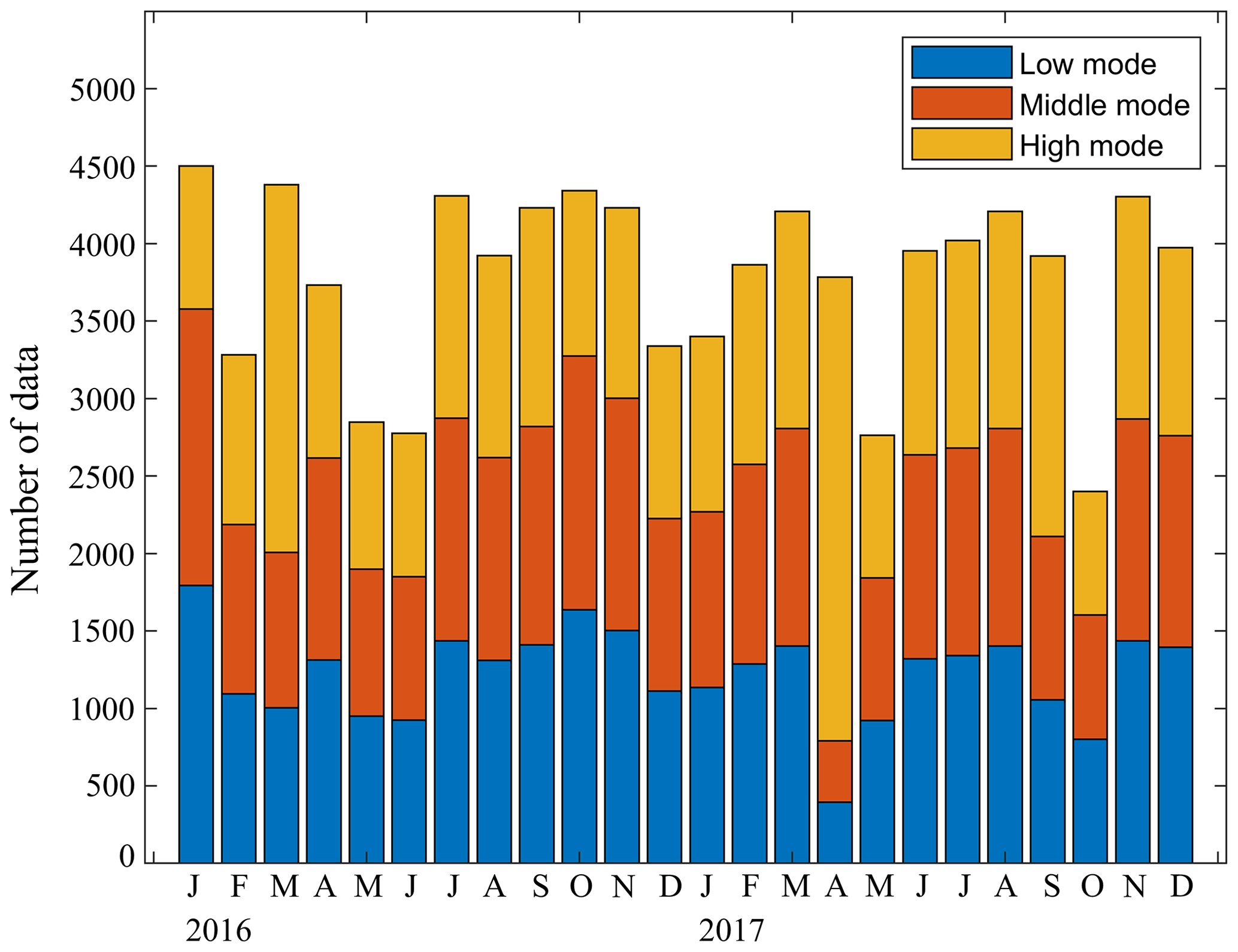
Figure 7The monthly total number of the Wuhan MST radar data in three observation modes during January 2016 to December 2017. Blue for low mode, red for middle mode, and orange for high mode.
3.1 Modes of operation
The Wuhan MST radar is used for the standard observations of the troposphere, lower stratosphere, and mesosphere in three observation modes: low mode (about 3.5–12 km), middle mode (about 10–25 km), and high mode (about 60–85 km). The height resolution is 150 m for the low mode, 600 m for the middle mode, and 1200 m for the high mode. Under normal operation, the system usually works in each mode for 5 min in sequence and then takes a break for 15 min. Hence, the wind data for each mode have a 30 min temporal resolution. The Wuhan MST radar was in good running condition during the full-time unattended operation from January 2016 to December 2017. Because of the system failures or external disturbances, severe interference may appear in some data (about 1 %). After removing the data with severe interference, the valid data set is present here to demonstrate the performance of the radar. Figure 7 shows the monthly total number of the Wuhan MST radar data in low, middle, and high modes. According to Fig. 7, the number of the radar data in most months exceeds 3000, except in March 2016, March 2017, and October 2017 during maintenance. On average, the number of daily mean data is 41 in low mode, 41 in middle mode, and 44 in high mode. In addition, the Wuhan MST radar took more observations of the mesosphere in March 2016 and April 2017. Therefore, the data set of the 2 years provides comprehensive and effective coverage of the troposphere, stratosphere, and mesosphere observations.
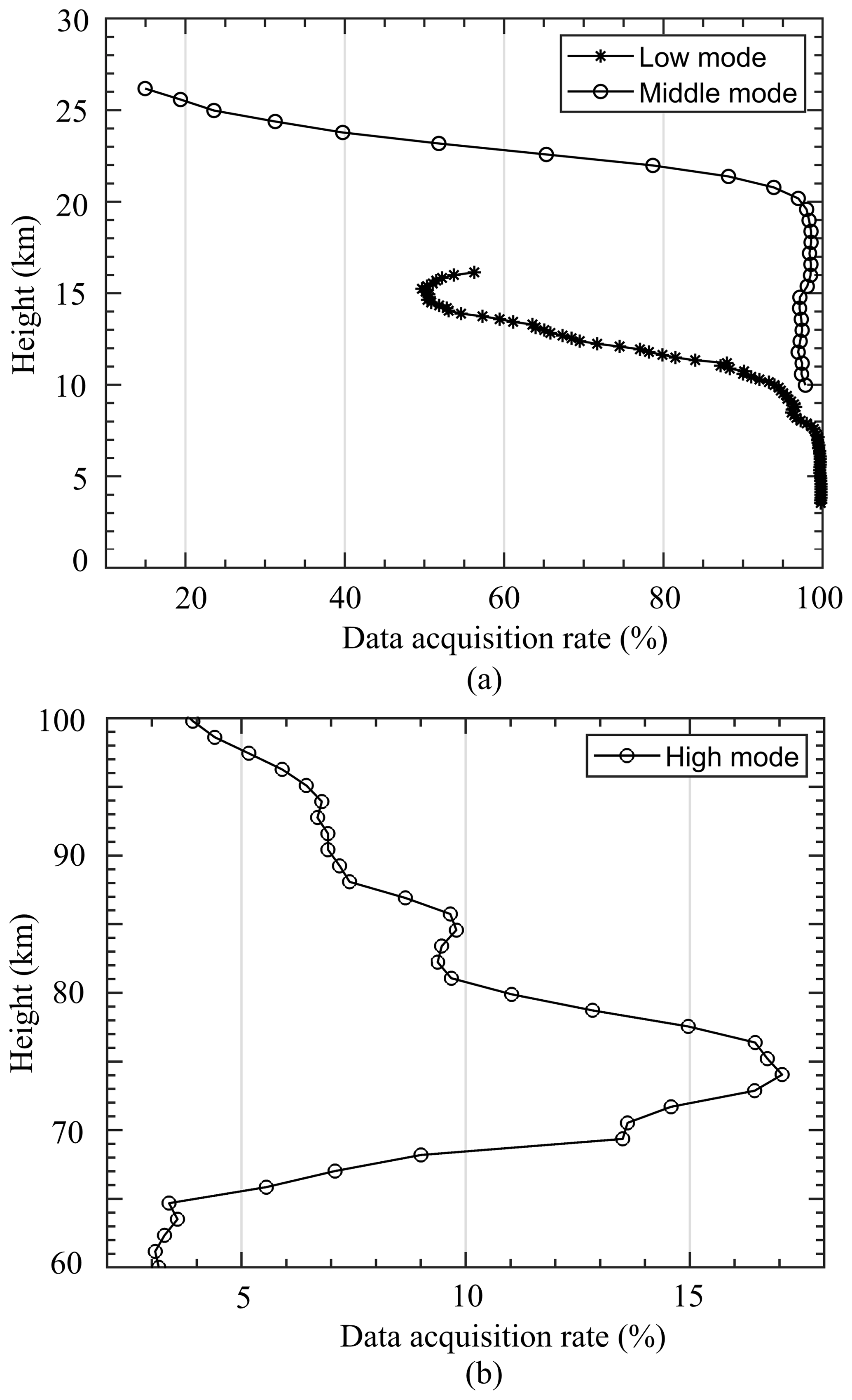
Figure 8The average data acquisition rate from the Wuhan MST radar in low and middle (a) and high (b) observation modes during January 2016 to December 2017.
3.2 Data acquisition
The data acquisition rate is one of the most important indices for describing the MST radar performance, which is calculated using the following relation: 100× number of samples with valid horizontal wind data / total number of samples (Kumar et al., 2007). The horizontal wind velocity is estimated by the radial velocity of the four inclined beams through the use of the Doppler beam swinging (DBS) technique (Anandan et al., 2001). If any one of the inclined beams has serious interference or a lower signal-to-noise (SNR) ratio, which leads to the failure of the horizontal wind velocity inversion, then the samples are judged to be invalid. Figure 8a shows the profile of total data acquisition in the low and middle mode during January 2016 to December 2017. In the low mode, the data acquisition rate remains >90 % at heights of 3.5–10 km and then decreases rapidly to 50 % at a height of 15 km. Note that the profile of the low mode clearly shows a reversal at heights of 14–16 km corresponding to the tropopause (Chen et al., 2019). In the middle mode, the data acquisition rate remains >90 % at heights of 10–20 km and then decreases rapidly to 19 % at a height of 25 km. Therefore, the connection height of the low mode and middle mode is usually selected at a height of 10 km for optimal data acquisition. In some situations which require a high range resolution, the data acquisition rate (>50 %) of the low mode is also available for the heights of 3.5–16 km.
As shown in Fig. 8b, the data acquisition rate of the high mode is mainly concentrated at heights of 66–86 km with a maximum up to 17 %, which is much lower than those of the low and middle modes. One reason for this is that the internal scales of neutral air turbulence in the mesosphere are mostly larger than half of the radio wavelength at the frequency of around 50 MHz (Hocking, 1985). Another reason is that the winds in the mesosphere are only available during the daytime (08:00–16:00 LT) in the D region (due to insufficient D region ionization during the nighttime; Rao et al., 2014). Actually, if the time range is limited in the daytime, the maximum data acquisition rate of the high mode is more than 50 %. The analysis of the data acquisition rate indicates that the Wuhan MST radar can receive the backscattered echoes from the troposphere, stratosphere, and mesosphere effectively.
3.3 Tropospheric and low stratospheric observation
In order to verify the validity of the wind measurements in the height ranges of 3.5–25 km, simultaneous observations obtained from the radiosonde were compared with the Wuhan MST radar observations. The radiosonde launch site (30.6∘ N, 114.1∘ E) is about 120 km away from the Wuhan MST radar, and the radiosonde was launched at 00:00 and 12:00 UT on 22 May 2016. It took about an hour for the balloon to rise up to 25 km, while the repetition period of the Wuhan MST radar is 30 min. Therefore, after the balloon was launched, the following two periods of the Wuhan MST radar data were averaged to compare them with the data from the radiosonde.
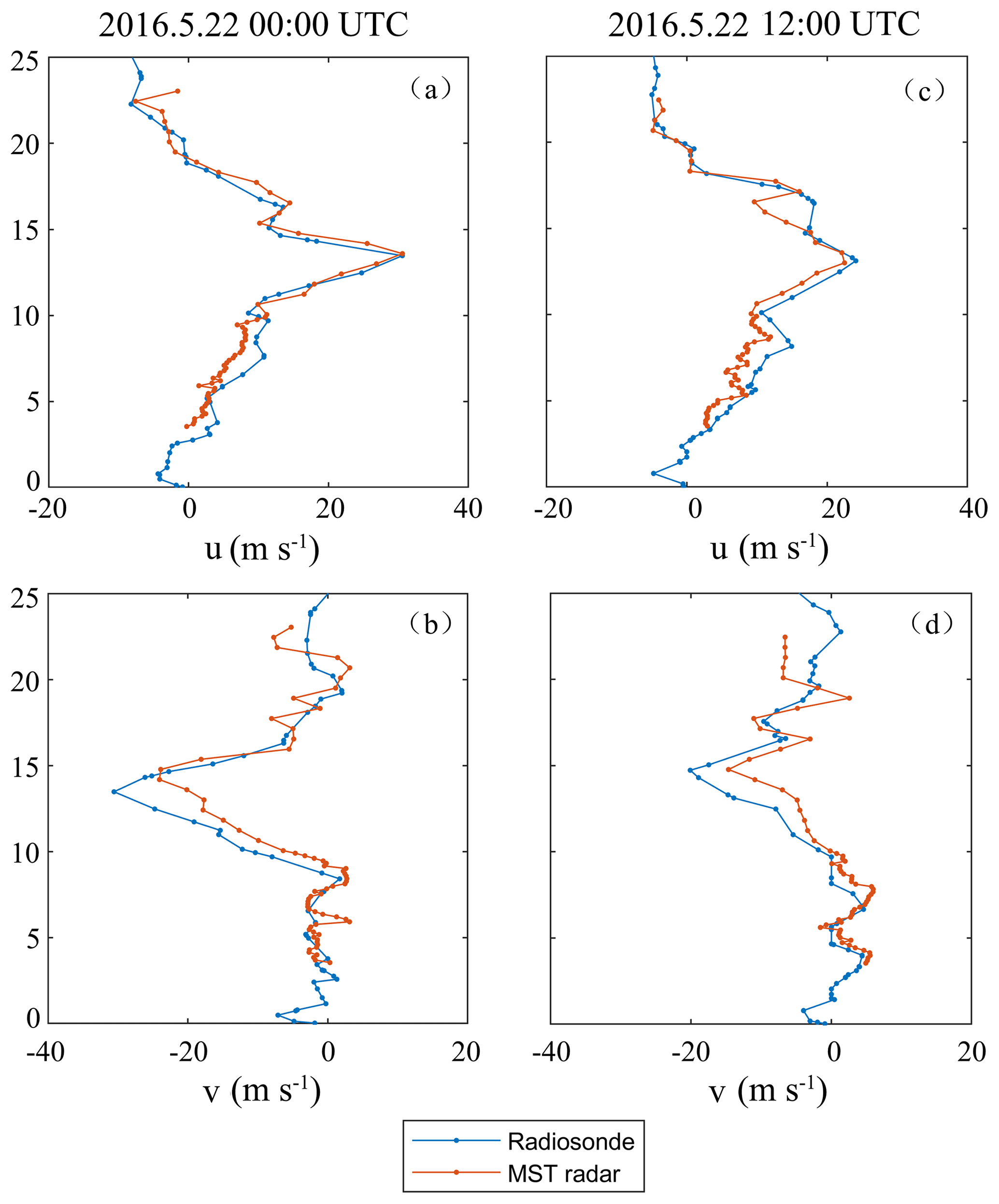
Figure 9The zonal (u) and meridional (v) winds at heights of 3.5–25 km observed by the Wuhan MST radar (red lines) and the radiosonde (blue lines) at 00:00 UT (a, b) and 12:00 UT (c, d) on 22 May 2016.
Note that since the balloon was detected at regular intervals by the tracking radar, the height resolution of the radiosonde is not uniform. Figure 9 shows the comparison of the zonal and meridional winds obtained by the Wuhan MST radar and the radiosonde launched at 00:00 and 12:00 UT on 22 May 2016. In these figures and throughout the paper, the positive zonal component corresponds to eastward wind, while the positive meridional component corresponds to northward wind. The zonal wind profiles are in good agreement in the altitude ranges of 3.5 to 23 km. The meridional wind profiles also show good agreement at most altitudes, but the winds observed by the Wuhan MST radar are weaker around the height of 14 km. The small discrepancies at some heights could be attributed to the variations in atmospheric activities at different temporal and spatial scales, and the different measurement principles and errors in both instruments are also significant reasons (Belu et al., 2010; Hocking, 2001).

Figure 10The contour plots of the monthly mean zonal (a) and meridional (c) winds in the troposphere and low stratosphere observed by the Wuhan MST radar during January 2016–December 2017. ERA-Interim model-estimated monthly mean zonal (b) and meridional (d) winds for the Wuhan region during the same period.
Figure 10 shows the contour plots of the monthly mean zonal and meridional winds in the troposphere and low stratosphere from the Wuhan MST radar and ERA-Interim. The observed mean winds are compared with ERA-Interim. ERA-Interim is one generation of European Centre for Medium-Range Weather Forecasts (ECMWF) global atmospheric reanalysis products, which offers good-quality atmospheric wind data with a 6 h temporal resolution and 3∘ × 3∘–0.125∘ × 0.125∘ latitude–longitude resolution (Dee et al., 2011; Houchi et al., 2010). The data set of monthly means of daily means is applied for the present study, which is produced by the average of the four main synoptic monthly means at 00:00, 06:00, 12:00, and 18:00 UTC (Berrisford et al., 2009).
It can be seen from Fig. 10a and b that the mean zonal wind observed by the Wuhan MST radar captures the major feature of ERA-Interim, which shows a clear annual oscillation with one westward jet and one eastward jet every year. The eastward jet occurs from September to June below ∼20 km, and the westward jet occurs from May to October above ∼20 km. The observed zonal winds in the eastward jet are ∼10 m s−1 weaker than the ERA-Interim reanalysis. The maximum magnitudes of the westward jet from the observation and the reanalysis are ∼14 and ∼20 m s−1, respectively. As shown in Fig. 10c and d, compared to the zonal winds, the meridional winds show larger discrepancies between the observation and the reanalysis. There are one northward jet and one southward jet exhibited in the observed mean meridional winds every year. The northward jet occurs from November to April below ∼18 km, and the southward jet occurs from May to September above ∼18 km. In ERA-Interim, the southward jets are extended in the 2 years. Especially in 2017, the southward jet occurs from April to October and extends down to a low height in April and May. According to the height resolution of the reanalysis data, the winds at altitudes of 3.48, 4.42, 4.94, 5.5, 6.71, 7.38, 8.81, 9.59, 10.42, 11.29, 12.21, 13.19, 15.33, 16.5, 19.05, 20.44, and 24.9 km from the Wuhan MST radar and ERA-Interim are analyzed. The correlation coefficients of 0.96 (zonal) and 0.7 (meridional) indicate the zonal winds have a more consistent trend, and the root mean square errors (RMSEs) of 9.3 (zonal) and 4 (meridional) indicate the meridional winds have a smaller deviation. Therefore, the larger correlation coefficient of the zonal winds may be attributed to the larger dynamic range. In conclusion, the Wuhan MST radar can measure the zonal and meridional winds in the troposphere and low stratosphere effectively.

Figure 11The daily mean zonal (u) and meridional (v) winds at heights of 76 to 86 km observed by the Wuhan MST radar (red lines) and the Wuhan meteor radar (blue lines) on 3 January 2016 (a, b), 12 January 2016 (c, d), and 13 January 2016 (e, f).
3.4 Mesospheric observation
In order to verify the validity of the mesospheric wind measurements, simultaneous observations obtained from the meteor radar at Wuhan were compared with the Wuhan MST radar observations. The Wuhan meteor radar (30.6∘ N, 114.4∘ E) is about 120 km away from the Wuhan MST radar and is an all-sky interferometric broadband radar system with a peak power of 7.5 kW and a frequency of 38.7 MHz (Xiong et al., 2004; Zhao et al., 2005). The averaging of daytime (08:00–16:00 LT) observations was used as the daily mean wind estimation for the Wuhan MST radar, while the 24 h average was used for the Wuhan meteor radar. Because of the effect of diurnal variations, the estimated mean winds of the Wuhan MST radar may be biased by less than 5 m s−1 compared with those of the Wuhan meteor radar below 85–90 km (Nakamura et al., 1996). Considering the observation height range of the two radars, the comparison range was set at heights of 76 to 86 km.
Figure 11 shows the daily mean zonal and meridional winds observed by the Wuhan MST radar and the Wuhan meteor radar on 3 individual days in January 2016. Interestingly, the measurements at a height of around 81 km show better agreement than at other heights, except for the meridional wind on 12 January 2016. This is because the measurements of the meteor radar are more reliable above 80 km (Venkat Ratnam et al., 2001; Kumar et al., 2008), while the data acquisition rate of the Wuhan MST radar is relatively high at heights of 70–85 km in the mesosphere. The zonal and meridional winds are of concordance in the aggregate. Two factors might result in the discrepancies between the observations of the two radars. The first one is localized gravity waves, tides, or planetary waves could cause the differences between them (Rao et al., 2014; Venkat Ratnam et al., 2001). The second is that the low data acquisition rate of the Wuhan MST radar in the mesosphere could lead to the fluctuations in the daily mean data, which show the sudden changes in the MST radar measurements at some heights.
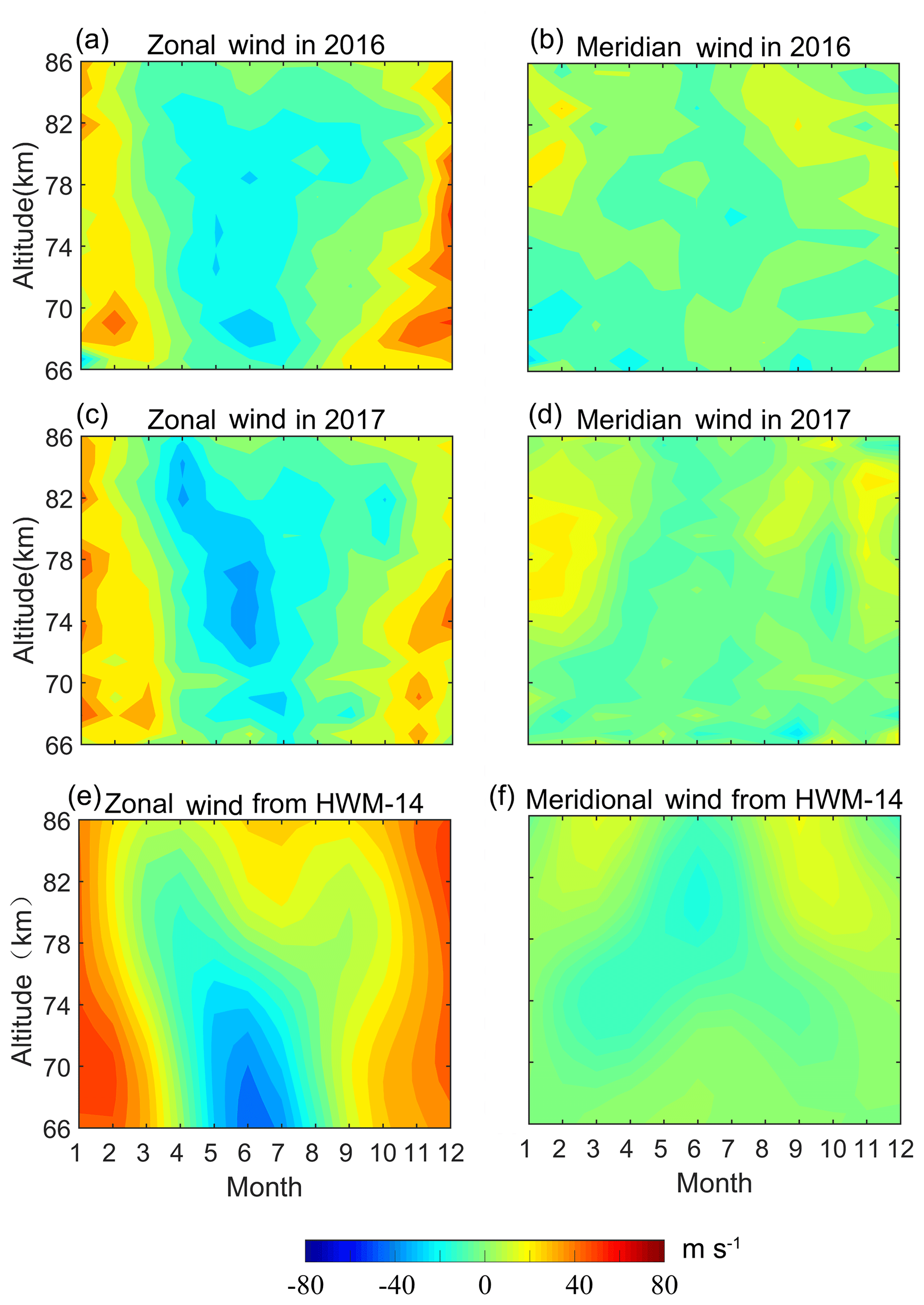
Figure 12The contour plots of the monthly mean zonal (a, c, e) and meridional (b, d, f) winds in the mesosphere observed by the Wuhan MST radar during January 2016–December 2016 and January 2017–December 2017. HWM-14 model-estimated winds (e, f) for Wuhan region during the same period.
Figure 12 shows contour plots of the monthly mean zonal and meridional winds from the MST radar and Horizontal Wind Model 14 (HWM-14). The observed mean winds are compared with the HWM-14. HWM-14, which is the upgraded version of HWM-07, is an empirical model that describes the atmosphere's vector wind fields from the surface to the exobase (∼450 km) as a function of latitude, longitude, altitude, day of year, and time of day (Drob et al., 2015).
As shown on the left side of Fig. 12, Wuhan MST radar zonal winds clearly show strong seasonal variations in 2016 and 2017. In general, the trends of the observational and predicted zonal winds match well, especially the reversal from eastward to westward in spring and the reversal from westward to eastward in autumn. However, HWM-14 overestimates the zonal winds in winter. Especially in February the magnitudes of the observational and predicted results have large differences. Many studies have indicated that stronger northward and westward winds happen after stratospheric sudden warming (SSW) events (Mbatha et al., 2010; Chau et al., 2015), and this factor is not considered in the HWM-14. The February 2016 SSW is a minor SSW, and the day of peak warming is on 5 February (Medvedeva and Ratovsky, 2017). Two minor warming events happened during the winter of 2017, with 2 d of peak warming on 2 and 26 February (Eswaraiah et al., 2019). The SSW events that happened during the observation period may influence the mean winds in the mesosphere. Hence, the stronger westward winds may result in smaller mean zonal winds during winter. Weakening and reversal in zonal winds observed between January and February can be found in Fig. S1 in the Supplement. Moreover, the differences in the zonal winds in summer are noticeable. The first difference is the reversal height in summer, which is a useful index for the mesopause. The wind shear at around 78 km is prominent during the summer from the HWM-14. Meanwhile, the reversal height observed by the Wuhan MST radar is about 84–85 km, which is consistent with the result observed by the MU radar at similar altitude (Namboothiri et al., 1999). Further study may be needed to analyze the difference. The second difference is the westward jet (the bluer region) that occurred in summer. There are some differences in the westward jet between the observations and predictions in occurrence time and height, which could be due to interannual variability. As seen from the right side of Fig. 12, it appears that the observational meridional winds of 2016 and 2017 have the same trend as the predicted results. They all have one northward jet that occurred above ∼75 km in the period from August to April, but the observational results are larger than the predicted results in winter because of the stronger northward winds during the SSW events. In general, the Wuhan MST radar wind measurements of the mesosphere are in agreement with the HWM-14 predictions in trend.
The technical features of the Wuhan MST radar are described in this paper. We use the TR modules and digital receiver with a smart structure and reasonable feeding network to realize the beam steering for three-dimensional wind field measurements. Wind observations of the Wuhan MST radar are compared with other instruments and related models for validation, and the results are summarized as follows:
-
Compared with the radiosonde (120 km away) and ERA-Interim, the zonal and meridional winds are in good agreement at heights of 3.5–25 km, and large discrepancies in meridional winds could be due to the temporal and spatial differences.
-
The daily mean zonal and meridional winds are in good agreement at heights of 76 to 86 km with the Wuhan meteor radar (120 km away), and the measurements at a height of around 81 km show better agreement than at other heights.
-
The monthly mean zonal and meridional winds are in agreement with the HWM in trend at heights of 66 to 86 km. The amplitudes of the observational results are different from those of the predicted results in winter, and this could be due to the influence of SSW events.
The comparisons indicate that the Wuhan MST radar is an effective tool to measure the three-dimensional wind fields of the MST region. These results encourage us to make further improvements, such as improving the data acquisition of the high mode and correcting the nominal zenith angle for the aspect sensitivity. In the future, we will use the Wuhan MST radar to study precipitation, gravity waves, and stratosphere–troposphere exchange processes during typhoons, cold fronts, or other events, as well as to study the dynamics of the mesosphere.
Wuhan MST radar data can be downloaded at https://data.meridianproject.ac.cn/instrument-option/?s_id=27 (last access: 6 July 2019; Meridian Project Data Center, 2020).
The supplement related to this article is available online at: https://doi.org/10.5194/amt-13-5697-2020-supplement.
LQ prepared the main part of the paper and performed the statistical analysis. GC is the project leader of the Wuhan MST radar and supported the preparation of the paper. SZ supervised the paper writing. QY implemented the construction work. The measurements were led by WG and FC. WZ and HZ helped with the statistical analysis of the Wuhan MST radar data. MS and EL provided valuable suggestion for data processing. The data analysis was supported by XC and HS. HZ and LZ edited the article.
The authors declare that they have no conflict of interest.
The authors would like to acknowledge the Chinese Meridian Project for the use of Wuhan MST radar data. This work is supported by the Natural Science Foundation of Zhejiang Province under grant LQ20D040001 and by the Chinese Meridian Project and National Natural Science Foundation of China under grant 41722404.
This research has been supported by the Natural Science Foundation of Zhejiang Province (grant no. LQ20D040001) and the National Natural Science Foundation of China (grant no. 41722404).
This paper was edited by Ad Stoffelen and reviewed by two anonymous referees.
Anandan, V. K., Reddy, G. R., and Rao, P. B.: Spectral analysis of atmospheric radar signal using higher order spectral estimation technique, IEEE T. Geosci. Remote, 39, 1890–1895, https://doi.org/10.1109/36.951079, 2001.
Balsley, B. B., Ecklund, W. L., Carter, D. A., and Johnston, P. E.: The MST radar at Poker Flat, Alaska, Radio Sci., 15, 213–223, https://doi.org/10.1029/RS015i002p00213, 1980.
Belu, R. G., Hocking, W. K., Donaldson, N., and Thayaparan, T.: Comparisons of CLOVAR windprofiler horizontal winds with radiosondes and CMC regional analyses, Atmos. Ocean, 39, 107–126, https://doi.org/10.1080/07055900.2001.9649669, 2010.
Berrisford, P., Dee, D. P., Poli, P., Brugge, R., Fielding, M., Fuentes, M., Kallberg, P. W., Kobayashi, S., Uppala, S., and Simmons, A.: The ERA-Interim Archive, ERA Report Series, 2009.
Chau, J. L., Hoffmann, P., Pedatella, N. M., Matthias, V., and Stober, G.: Upper mesospheric lunar tides over middle and high latitudes during sudden stratospheric warming events, J. Geophys. Res., 120, 3084–3096, https://doi.org/10.1002/2015JA020998, 2015.
Chen, F., Chen, G., Tian, Y., Zhang, S., Huang, K., Wu, C., and Zhang, W.: High-resolution Beijing mesosphere–stratosphere–troposphere (MST) radar detection of tropopause structure and variability over Xianghe (39.75∘ N, 116.96∘ E), China, Ann. Geophys., 37, 631–643, https://doi.org/10.5194/angeo-37-631-2019, 2019.
Chen, G., Cui, X., Chen, F., Zhao, Z., Wang, Y., Yao, Q., Wang, C., Lü, D., Zhang, S., Zhang, X., Zhou, X., Huang, L., and Gong, W.: MST Radars of Chinese Meridian Project: System Description and Atmospheric Wind Measurement, IEEE T. Geosci. Remote, 54, 4513–4523, https://doi.org/10.1109/TGRS.2016.2543507, 2016.
Chilson, P. B., Kirkwood, S., and Nilsson, A.: The Esrange MST radar: A brief introduction and procedure for range validation using balloons, Radio Sci., 34, 427–436, https://doi.org/10.1029/1998rs900023, 1999.
Chu, Y. and Yang, K.: Reconstruction of spatial structure of thin layer in sporadic E region by using VHF coherent scatter radar, Radio Sci., 44, RS5003, https://doi.org/10.1029/2008RS003911, 2009.
Dee, D. P., Uppala, S. M., Simmons, A. J., Berrisford, P., Poli, P., Kobayashi, S., Andrae, U., Balmaseda, M. A., Balsamo, G., Bauer, P., Bechtold, P., Beljaars, A. C. M., Berg, L., Bidlot, J., Bormann, N., Delsol, C., Dragani, R., Fuentes, M., Geer, A. J., Haimberger, L., Healy, S. B., Hersbach, H., Holm, E. V., Isaksen, L., Kallberg, P., Kohler, M., Matricardi, M., McNally, A. P., Monge-Sanz, B. M., Morcrette, J.-J., Park, B.-K., Peubey, C., Rosnay, P., Tavolato, C., Thepaut, J.-N., and Vitart, F.: The ERA-Interim reanalysis: configuration and performance of the data assimilation system, Q. J. Roy. Meteor. Soc., 137, 553–597, https://doi.org/10.1002/qj.828, 2011.
Drob, D. P., Emmert, J. T., Meriwether, J. W., Makela, J. J., Doornbos, E., Conde, M., Hernandez, G., Noto, J., Zawdie, K. A., McDonald, S. E., Huba, J. D., and Klenzing, J. H.: An update to the Horizontal Wind Model (HWM): The quiet time thermosphere, Earth Space Science, 2, 301–319, https://doi.org/10.1002/2014EA000089, 2015.
Eswaraiah, S., Ratnam, M. V., Kim, Y. H., Kumar, K. N., Chalapathi, G. V., Ramanajaneyulu, L., Lee, J., Prasanth, P. V., and Thyagarajan, S. V. B.: Advanced meteor radar observations of mesospheric dynamics during 2017 minor SSW over the tropical region, Adv. Space Res., 64, 1940–1947, https://doi.org/10.1016/j.asr.2019.05.039, 2019.
Fukao, S., Tsuda, T., Sato, T., Kato, S., Wakasugi, K., and Makihira, T.: The mu radar with an active phased array system: 1. Antenna and power amplifiers, Radio Sci., 20, 1155–1168, https://doi.org/10.1029/rs020i006p01155, 1985.
Fukao, S., Hashiguchi, H., Yamamoto, M., Tsuda, T., Nakamura, T., and Yamamoto, M. K.: Equatorial Atmosphere Radar (EAR): System description and first results, Radio Sci., 38, 19-1–19-17, https://doi.org/10.1029/2002RS002767, 2003.
Green, J. L., Gage, K. S., and Van Zandt, T. E.: Atmospheric measurements by VHF pulsed Doppler radar, IEEE Trans. Geosci. Electron., GE-17, 262–280, https://doi.org/10.1109/TGE.1979.294655, 1979.
Hocking, W. K.: Measurement of turbulent energy dissipation rates in the middle atmosphere by radar techniques: A review, Radio Sci., 20, 1403–1422, https://doi.org/10.1029/rs020i006p01403, 1985.
Hocking, W. K.: VHF tropospheric scatterer anisotropy at Resolute Bay and its implications for tropospheric radar-derived wind accuracies, Radio Sci., 36, 1777–1793, https://doi.org/10.1029/2000rs001002, 2001.
Hocking, A. A.: A review of Mesosphere–Stratosphere–Troposphere (MST) radar developments and studies, circa 1997–2008, J. Atmos. Sci., 73, 848–882, https://doi.org/10.1016/j.jastp.2010.12.009, 2011.
Hooper, D. A., Bradford, J., Dean, L., Eastment, J. D., Hess, M., Hibbett, E., Jacobs, J., and Mayo, R.: Renovation of the Aberystwyth MST radar: evaluation, in: Proceedings of the Thirteenth International Workshop on Technical and Scientific Aspects of MST Radar, Leibniz-Institute of Atmospheric Physics at the Rostock University, Kühlungsborn, Germany, 86–90, 2013.
Houchi, K., Stoffelen, A., Marseille, G. J., and De Kloe, J.: Comparison of wind and wind shear climatologies derived from high-resolution radiosondes and the ECMWF model, J. Geophys. Res., 115, D22123, https://doi.org/10.1029/2009jd013196, 2010.
Kawahigashi, H., Kato, S., Kimura, I., Tsuda, T., Sato, T., and Yamamoto, M.: History of Development of the MU (Middle and Upper Atmosphere) Radar, the First Large-Scale Atmospheric Radar with Two-Dimensional Active Phased Array Antenna System, 2017 IEEE HISTory of ELectrotechnolgy CONference (HISTELCON), Kobe, 47–52, https://doi.org/10.1109/HISTELCON.2017.8535930, 2017.
Kumar, G. K., Ratnam, M. V., Patra, A. K., Rao, V. V. M. J., Rao, S. V. B., and Rao, D. N.: Climatology of low-latitude mesospheric echo characteristics observed by Indian mesosphere, stratosphere, and troposphere radar, J. Geophys. Res., 112, D06109, https://doi.org/10.1029/2006JD007609, 2007.
Kumar, G. K., Ratnam, M. V., Patra, A. K., Rao, V. V. M. J., Rao, S. V. B., Kumar, K. K., Gurubaran, S., Ramkumar, G., and Rao, D. N.: Low-latitude mesospheric mean winds observed by Gadanki mesosphere-stratosphere-troposphere (MST) radar and comparison with rocket, High Resolution Doppler Imager (HRDI), and MF radar measurements and HWM93, J. Geophys. Res., 113, D19117, https://doi.org/10.1029/2008JD009862, 2008.
Kumar, S., Rao, T. N., and Radhakrishna, B.: Identification and Separation of Turbulence Echo From the Multipeaked VHF Radar Spectra During Precipitation, IEEE T. Geosci. Remote., 57, 5729–5737, https://doi.org/10.1109/TGRS.2019.2901832, 2019.
Latteck, R., Singer, W., Rapp, M., Vandepeer, B., Renkwitz, T., Zecha, M., and Stober, G.: MAARSY: The new MST radar on Andøya – System description and first results, Radio Sci., 47, 222–237, https://doi.org/10.1029/2011RS004775, 2012.
Mbatha, N., Sivakumar, V., Malinga, S. B., Bencherif, H., and Pillay, S. R.: Study on the impact of sudden stratosphere warming in the upper mesosphere–lower thermosphere regions using satellite and HF radar measurements, Atmos. Chem. Phys., 10, 3397–3404, https://doi.org/10.5194/acp-10-3397-2010, 2010.
Medvedeva, I. and Ratovsky, K.: Effects of the 2016 February minor sudden stratospheric warming on the MLT and ionosphere over Eastern Siberia, J. Atmos. Solar-Terr. Phy., 180, 116–125, https://doi.org/10.1016/j.jastp.2017.09.007, 2017.
Meridian Project Data Center: Meridian project, available at: https://data.meridianproject.ac.cn/instrument-option/?s_id=27 (last access: 6 July 2019), 2020.
Nakamura, T., Tsuda, T., and Fukao, S.: Mean winds at 60–90 km observed with the MU radar (35∘ N), J. Atmos. Sci., 58, 655–660, https://doi.org/10.1016/0021-9169(95)00064-X, 1996.
Namboothiri, S. P., Tsuda, T., and Nakamura, T.: Interannual variability of mesospheric mean winds observed with the MU radar, J. Atmos. Sci., 61, 1111–1122, https://doi.org/10.1016/S1364-6826(99)00076-0, 1999.
Rao, P. B., Jain, A. R., Kishore, P., Balamuralidhar, P., Damle, S. H., and Viswanathan, G.: Indian MST radar 1. System description and sample vector wind measurements in ST mode, Radio Sci., 30, 1125–1138, https://doi.org/10.1029/95RS00787, 1995.
Rao, Q., Hashiguchi, H., and Fukao, S.: Study on ground clutter prevention fences for boundary layer radars, Radio Sci., 38, 13-1–13-15, https://doi.org/10.1029/2001rs002489, 2003.
Rao, S. V. B., Eswaraiah, S., Ratnam, M. V., Kosalendra, E., Kumar, K. K., Kumar, S. S., Patil, P. T., and Gurubaran, S.: Advanced meteor radar installed at Tirupati: System details and comparison with different radars, J. Geophys. Res., 119, 11893–11904, https://doi.org/10.1002/2014JD021781, 2014.
Rottger, J., Liu, C. H., Chao, J. K., Chen, A. J., Chu, Y. H., Fu, I.-J., Huang, C. M., Kiang, Y. W., Kuo, F. S., Lin C. H., and Pan C. J.: The Chung-Li VHF radar: Technical layout and a summary of initial results, Radio Sci., 25, 487–502, https://doi.org/10.1029/RS025i004p00487, 1990.
Sato, K., Tsutsumi, M., Sato, T., Nakamura, T., Saito, A., Tomikawa, Y., Nishimura, K., Kohma, M., Yamagishi, H., and Yamanouchi, T.: Program of the Antarctic Syowa MST/IS radar (PANSY), J. Atmos. Sci., 118, 2–15, https://doi.org/10.1016/j.jastp.2013.08.022, 2014.
Schmidt, G., Ruster, R., and Czechowsky, P.: Complementary Code and Digital Filtering for Detection of Weak VHF Radar Signals from the Mesosphere, IEEE Trans. Geosci. Electron., 17, 154–161, https://doi.org/10.1109/tge.1979.294643, 1979.
Vaughan, G.: The UK MST radar, Weather, 57, 69–73, https://doi.org/10.1002/wea.6080570206, 2002.
Venkat Ratnam, M., Narayana Rao, D., Narayana Rao, T., Thulasiraman, S., Nee, J. B., Gurubaran, S., and Rajaram, R.: Mean winds observed with Indian MST radar over tropical mesosphere and comparison with various techniques, Ann. Geophys., 19, 1027–1038, https://doi.org/10.5194/angeo-19-1027-2001, 2001.
Wang, C.: Development of the Chinese Meridian Project, Chin. J. Space. Sci., 30, 382–384, https://doi.org/10.1360/972009-470, 2010.
Woodman, R. F. and Guillen, A.: Radar observations of winds and turbulence in the stratosphere and mesosphere, J. Atmos. Sci., 31, 493–505, https://doi.org/10.1175/1520-0469(1974)031<0493:ROOWAT>2.0.CO;2, 1974.
Xiong, J. G., Wan, W., Ning, B., and Liu, L.: First results of the tidal structure in the MLT revealed by Wuhan Meteor Radar (30∘40′ N, 114∘30′ E), J. Atmos. Sci., 66, 675–682, https://doi.org/10.1016/j.jastp.2004.01.018, 2004.
Zhao, G., Liu, L., Wan, W., Ning, B., and Xiong, J.: Seasonal behavior of meteor radar winds over Wuhan, Earth Planets Space, 57, 393–398, https://doi.org/10.1186/BF03351806, 2005.