the Creative Commons Attribution 4.0 License.
the Creative Commons Attribution 4.0 License.
 | 27 Oct 2020
Inter-calibration of nine UV sensing instruments over Antarctica and Greenland since 1980
Clark J. Weaver
Pawan K. Bhartia
Dong L. Wu
Gordon J. Labow
David E. Haffner
Nadir-viewed intensities (radiances) from nine UV sensing satellite instruments are calibrated over the East Antarctic Plateau and Greenland during summer. The calibrated radiances from these UV instruments ultimately will provide a global long-term record of cloud trends and cloud response from ENSO events since 1980. We first remove the strong solar zenith angle dependence from the intensities using an empirical approach rather than a radiative transfer model. Then small multiplicative adjustments are made to these solar zenith angle normalized intensities in order to minimize differences when two or more instruments temporally overlap. While the calibrated intensities show a negligible long-term trend over Antarctica and a statistically insignificant UV albedo trend of −0.05 % per decade over the interior of Greenland, there are small episodic reductions in intensities which are often seen by multiple instruments. Three of these darkening events are explained by boreal forest. Other events are caused by surface melting or volcanoes. We estimate a 2-sigma uncertainty of 0.35 % for the calibrated radiances.
- Article
(5746 KB) - Full-text XML
- BibTeX
- EndNote


In 1978 the Nimbus-7 spacecraft carried the first Solar Backscatter in the UV (SBUV) instrument into low earth orbit to measure total column ozone. Since then, NOAA has deployed a suite of SBUV-2 instruments onboard the NOAA-9, -11, -14, -16, -17, -18 and -19 spacecraft. Since they were all nadir viewing and thus had limited spatial coverage, NASA also deployed a suite of mapping instruments: Nimbus-7 TOMS, Earth Probe TOMS and the Nadir Mapper (NM) instrument of the Suomi NPP Ozone Mapping Profiler Suite (OMPS). True to their design, they have provided a long-term satellite data record of ozone products; however, they also were intended to measure the earth's reflectivity in the UV at wavelengths insensitive to ozone (331 and 340 nm). Aside from a few publications (Herman et al., 2013; Labow et al., 2011; Weaver et al., 2015), this data set has not been fully exploited. Our ultimate goal is a long-term record of a UV cloud product that can be directly compared with climate models. This paper details the first step: the inter-calibration of radiances from the suite of nadir-viewing instruments. The second step retrieves a black-sky cloud albedo (BCA) record from the inter-calibrated intensities (Weaver et al., 2020) and compares the BCA with the shortwave CERES cloud albedo.
The backbone of our data record is the suite of eight SBUV instruments starting with Nimbus-7 in 1980 and ending with NOAA-19 in 2013. Thereafter we use the NM instrument on the Suomi NPP OMPS. Each instrument provides narrowband backscattered intensities near the 340 nm wavelength. We use a radiative transfer model to account for the small differences in each instrument's center wavelength (see Appendix). Regular sun-viewing irradiance measurements (Fsun) are made, typically weekly, to provide long-term calibration information. The measured intensities are normalized by Fsun and multiplied by π. Throughout this study I refers to the sun-normalized intensities.
We start with intensities that have already been calibrated to account for instrument effects such as hysteresis (see DeLand et al., 2012) and that are reported in the Level-2 data sets for each instrument. The first seven SBUV/2 data sets were previously calibrated by characterizing the instruments over the East Antarctic Plateau ice sheet using Lambertian equivalent reflectivity (LER, Huang et al., 2003; Herman et al., 2013). Using a radiative transfer model to calculate LER from the observed intensities removes much of the solar zenith angle (θo) dependence but not all; over the ice sheets LER still decreases with θo, especially at high θo. While they did an excellent job of characterizing the first seven SBUV/2 instruments, two additional sensors need to be inter-calibrated to extend our record forward: the SBUV2 on NOAA-19 and the Suomi NPP OMPS. Rather than calibrate these additional instruments with a radiative transfer model using LER, we use an empirical approach to remove the solar zenith angle dependence on intensity. Using these θo-normalized intensities, we inter-calibrate the UV sensors over the East Antarctic Plateau and the Greenland Ice Sheet.
Satellite-observed nadir-viewed intensities over the Antarctic and Greenland ice sheets have an almost linear relationship with solar zenith angle that is easily fitted with a 5-degree polynomial. Figure 1 shows the relationship over both ice sheets for all observations sampled by the SBUV2 on NOAA-16. With a drifting orbit and long lifetime (2001–2014) NOAA-16 sampled a wide range of solar zenith angles, so we choose it as our reference instrument. The polynomial fit uses all observations over the instrument's 14-year lifetime and so provides a most probable intensity that the NOAA-16 SBUV2 would observe for a given θo. Our calibration approach is to remove the solar zenith angle dependence from the observed intensities (Iobs) by using the reference polynomial fits shown in Fig. 1. We can test whether an observed intensity is high or low compared with the NOAA-16 SBUV2 reference by calculating a fractional deviation in terms of intensity (δI) from Eq. (1). For example, the right panel of Fig. 1 shows an anomalously low intensity sampled over a dark scene ( observed at a solar zenith angle (; it is compared with the intensity that NOAA-16 would likely have observed at that solar zenith angle (ξ ()). The difference is divided by ξ ( to produce a fractional deviation in intensity δI which is common throughout the paper.
Each UV instrument has its own unique Iobs to θo relationship mainly because the photomultiplier tube (PMT) for each instrument has a slightly different response function. The underlying scene UV albedo (averaged over an instrument's lifetime) could be slightly different for each instrument, which would also change the Iobs to θo relationship, but we expect the Antarctic Plateau albedo to be stable over time. The SBUV PMTs are designed to have a zero-offset bias, i.e., zero current response when there are zero photon counts. Although the polynomial fit is not constrained to have Iobs=0 at a solar zenith angle of 90∘, it appears so, consistent with this instrument design (Fig. 1).
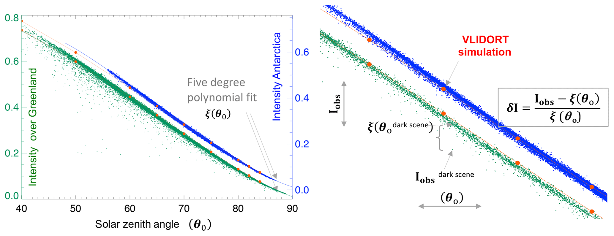
Figure 1Measured intensity at 340 nm from the NOAA-16 SBUV versus solar zenith angle over the Antarctic Plateau (blue) and Greenland (green). Each point is a nadir-viewed observation at the native field of view (170 km by 170 km) during the summer (15 d on either side of solstice). Also shown is a polynomial fit and a radiative transfer simulation (red) assuming a Lambertian surface albedo of 0.95 and a Rayleigh atmosphere with a surface pressure of 663 hPa. Note that the Greenland intensities are offset from the Antarctic ones. The right panel shows a zoomed-in view (see text for details).
We also show estimates of intensity calculated by the VLIDORT (Vector LInearized Discrete Ordinate Radiative Transfer package, Spurr, 2006) radiative transfer model. Here we assume Lambertian surface albedo of 0.95 and Rayleigh atmosphere with surface pressure of 663 hPa. The number of half-space quadrature streams is 40; the number of Stokes vector parameters is 3. At first glance the VLIDORT simulation appears to simulate the observations (red trace Fig. 1), and we considered using the I-to-θo relationship simulated by VLIDORT as a reference (instead of using NOAA-16), but closer examination shows that the slope of VLIDORT is shallow compared with the observations. The resulting δI would still be slightly dependent on θo, which would complicate the analysis.
Another, more sophisticated approach to validate sun-normalized radiances over ice sheets is described in Jaross and Warner (2008) They account for snow surface BRDF and off-nadir viewing angles. Nadir 330 nm reflectances simulated using their snow BRDF model are 1 % less than those assuming a Lambertian surface at θo=70∘; disparities are near zero at θo=50∘. Our nadir-observed δI is not sensitive to solar azimuth angle over Antarctica.
The suite of SBUV/2 instruments provides nadir observations with a 170×170 km field of view (FOV), but the OMPS Mapper instrument has a smaller nominal 50×50 km FOV except at the two most nadir-viewing positions. Here the FOV widths are 20 and 30 km (Seftor el al., 2014). For consistency, we only used the Mapper viewing positions that were within a nadir-centered hypothetical 170×170 km SBUV FOV and aggregated their intensities (area weighted) prior to calculating δI. For each instrument we calculate the summertime annual mean and plot the time series for both ice sheets (Fig. 2).
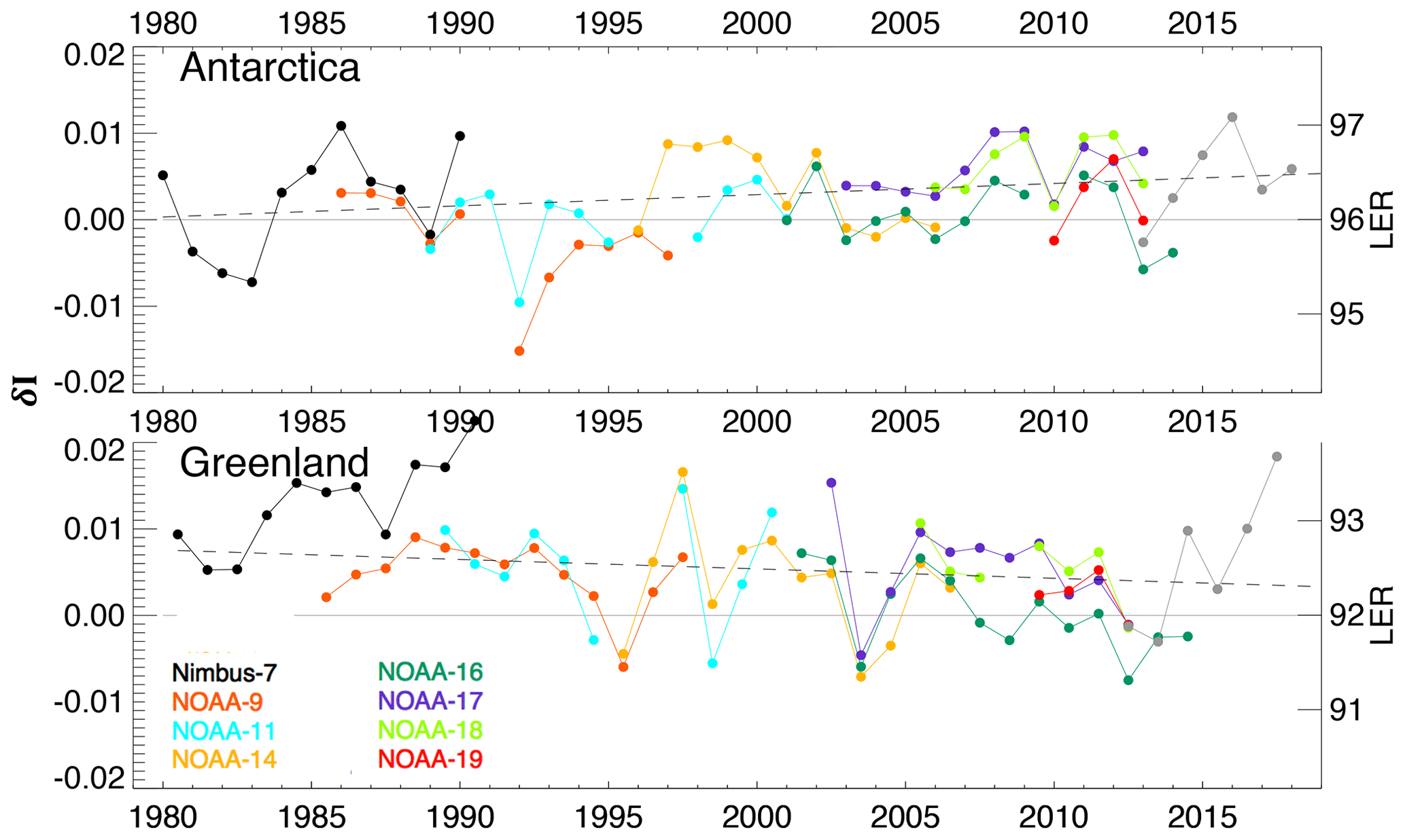
Figure 2Inter-annual variability of previously calibrated δI for the SBUV instruments (colored) and OMPS Mapper (grey) over Antarctica and Greenland. The right-hand axis shows the corresponding change in LER.
The pre-calibrated intensity SBUV2 instruments onboard NOAA-17, -18 and -19 appear to be high biased compared to our reference (Fig. 2). As described below, a cost-optimization approach is used to adjust the intensities and reduce these disparities. Figure 2 only shows the summertime average δI, but when calibrating instruments, it is instructive to examine the δI dependence on θo for individual years. The left panel of Fig. 3a shows this for 2006 when the reference and three other instruments were operational. The positive bias for NOAA-17 and -18 is consistent at all θo bins and suggests that a simple adjustment of the intensities might reduce these biases. All instruments show a similar skewed δI distribution, at each θo bin, toward low values of δI.
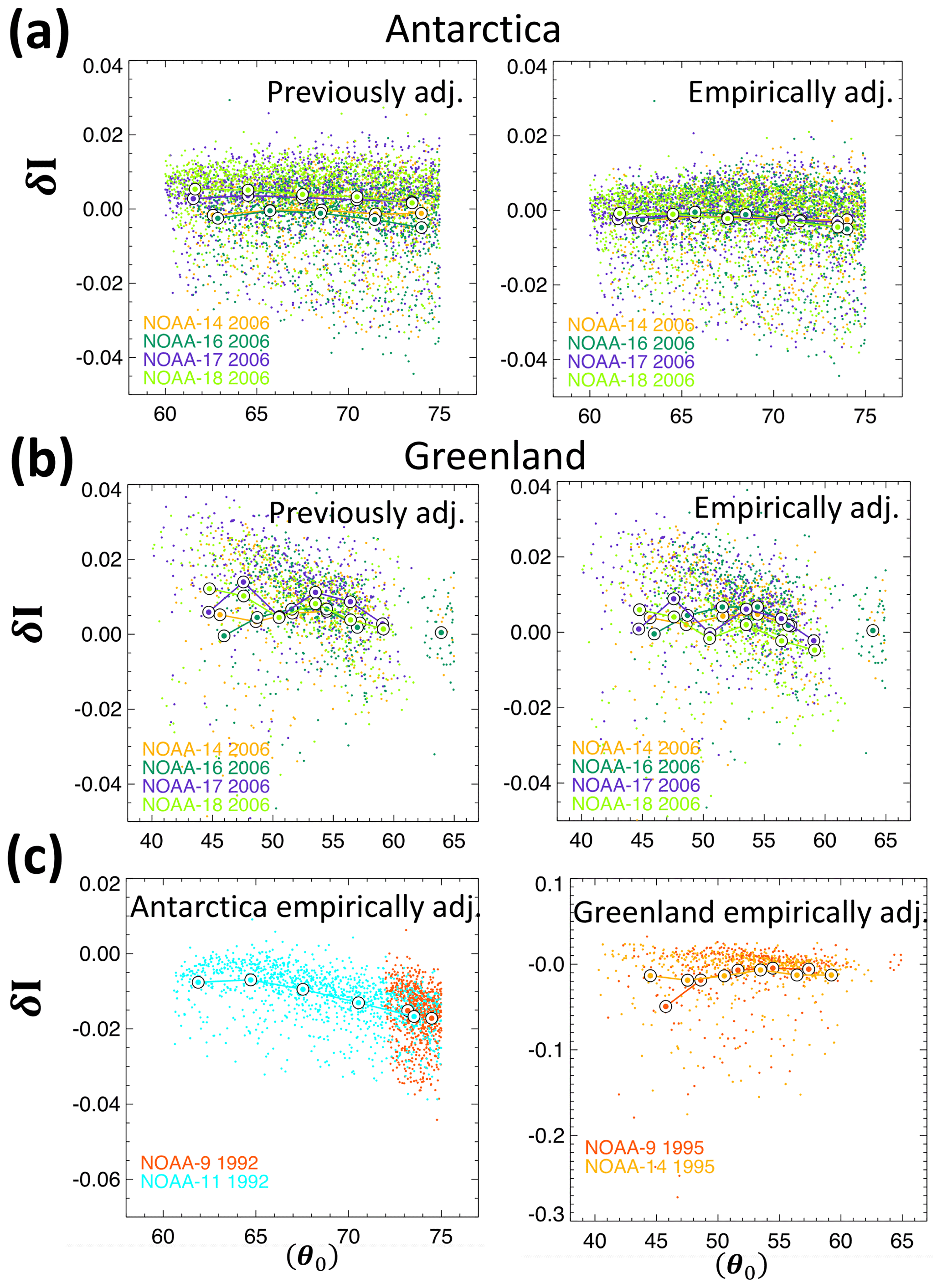
Figure 3δI for all FOVs observed over the ice sheets plotted against solar zenith angle (θo) for specific years. The large circles are averages of δI binned by solar zenith angle. Panel (a) shows the previously calibrated δI on the left and our empirically calibrated δI over Antarctica on the right for 2006. Panel (b) is the same but over Greenland for 2006. Panel (c) shows our empirically calibrated values over Antarctica in 1992 and Greenland in 1995.
To adjust intensities for a specific instrument, a multiplicative factor (c1) is chosen so that the adjusted intensities are a linear function of the original intensities: . Adjusting the multiplicative factor (c1) changes the gain (intensity per observed photon counts) of the instrument. To inter-calibrate all instruments with respect to NOAA-16, we use a minimum-cost optimization algorithm to solve for a set of c1 values that minimizes δI disparities between temporally overlapping instruments. The c1 for each instrument, except the reference, is allowed to vary; Table 1 shows the gain changes made to each instrument. Note that c1 does not depend on time, so the interannual variability of a specific SBUV instrument remains intact after the calibration.
Table 1Gain c1 and offset c0 values used to make adjustments to observed intensities using the linear equation .

Only the highest-quality observations are used for the inter-calibration. Observations are limited to θo less than 75∘ because at higher θo ozone absorption and straylight effects become significant and contaminate results. Furthermore, SBUV observations that have a grating drive error and observations that are likely impacted by PMT hysteresis are not used to inter-calibrate.
The grating drive selects the wavelength of a SBUV measurement. Sometimes, but not too often, the grating drive selects the wrong value and the intensities are measured at a wavelength different than the SBUV instrument's nominal wavelength. Inclusion of observations with uncorrected grating errors will confuse our results, since our analysis assumes that intensities to derive δI are all at the same wavelength. Fortunately, the grating drive position is archived, so we can apply a correction (see Appendix); however, the observations with uncorrected grating errors are not used in the inter-calibration but are used in the later trend analysis. Figure 4 shows the summertime average empirically adjusted δI over both ice sheets after applying the gain changes in Table 1. Solid circles exclude observations with grating drive errors and open circles include corrected observations. There is clearly a tighter match between overlapping instruments compared with Fig. 2, but there still are disparities between overlapping instruments between 1997 and 1999, when multiple instruments suffer from grating errors. It is disconcerting that our correction does not bring them into closer alignment.

Figure 4Inter-annual variability of our δI for the SBUV instruments (colored) and the OMPS Mapper (grey) over Antarctica (a) and interior locations over Greenland with ice surface elevations above 2000 m (b). The right-hand axis shows the corresponding change in LER. Annual means plotted with solid circles only include observations with correct grating drive positions; open circles also include those with grating drive errors that have been corrected (see text). The lowest panel (Fig. 4c) shows MODIS Collection 6 reflectance for Band 3 (459 nm) at elevations above 2000 m (dry snow conditions dashed trace) and below 2000 m (wet snow conditions solid trace).
Both Nimbus-7 and, to a lesser extent, NOAA-9 suffered from PMT hysteresis. These earlier PMTs were not able to quickly respond to the 4 orders of magnitude signal changes that occur when the satellite first comes out of darkness on each orbit and the instrument sees its first light. For Nimbus-7 hysteresis errors are between 4 % and 9 % at first light over Antarctica and lessen as the PMT adjusts to the bright scenes over the ice sheet. By the time Nimbus-7 reaches Greenland the PMT is equilibrated and there is no hysteresis error (maximum hysteresis errors of NOAA-9 are 2 %). The intensity observations for these early instruments have been corrected for hysteresis (DeLand et al., 2001). Still, we initially were unable to match Nimbus-7 with the other instruments; there was good agreement over Antarctica, but over Greenland Nimbus-7 was about 1 % higher than the others (Fig. 2).
Our remedy was to first calibrate the SBUV instruments only over Greenland where Nimbus-7 is free of hysteresis error. As expected, all temporally overlapping instruments agreed over Greenland, but over Antarctica Nimbus-7 was low by about 1 % compared with NOAA-9 and NOAA-11. Then we started removing Nimbus-7 observations: first those within 1 min of first light, and then 2 min. With every minute of observations removed, the disparity over Antarctica lessened. We achieved the good agreement seen in Fig. 4 by removing 9 min of Nimbus-7 observations after first light.
Figure 5 shows the θo dependence on the empirically adjusted δI for selected years. All the SBUVs, except for Nimbus-7 and NOAA-9, have an almost flat (<0.005) δI dependence with θo. A flat θo dependence indicates that the PMT response is similar to the NOAA-16. Over Greenland δI dependence with θo is not quite as flat (Fig. 3b). Over Antarctica the suppression of δI at θo>57∘ and time after first light <9 min is seen for all years of Nimbus-7. Even though these suppressed observations (θo>57∘) were previously corrected for hysteresis, artifacts remain, and they are not used in any analysis.
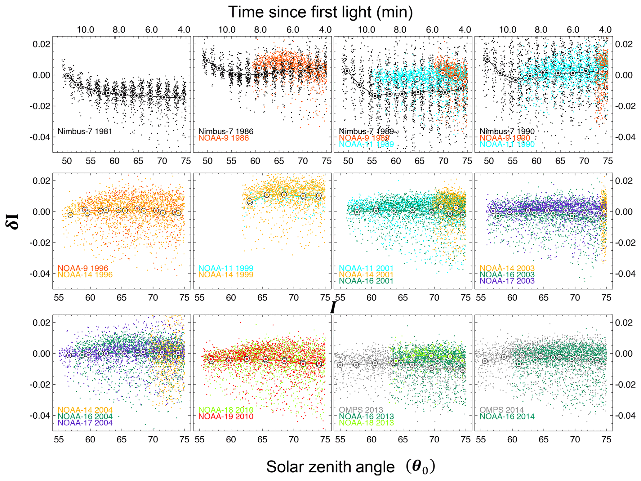
Figure 5Empirically calibrated δI for all FOVs observed over Antarctica plotted against solar zenith angle (θo) for selected years. The top four panels show the suppression of δI during the first 7–10 min after Nimbus-7 sees its first light at the start of a new orbit. At first light, time = 0 and θo=90∘. The time after first light (minutes) is shown at the top of the first four panels.
Two instruments show coincident reduction of δI over Antarctica in January 1992 (Fig. 4), most likely from aerosols transported to the Antarctic after the eruption of Mt. Pinatubo 6 months earlier in 1991 (left panel of Fig. 3c). The April 1982 eruption of El Chichon likely contributed to the coincident reduction in 1983; other anomalies occur in 2001, 2010 and 2013. Likewise, there are coincident reductions in δI over Greenland.
To estimate the uncertainty in the SBUV intensity from instrument calibration alone, we first average the δI over the coincident satellites for each year; this merged time series represents the geophysical contribution. Absolute departures from this merged time series (Fig. 6) are attributed to instrument calibration uncertainty. Two times the standard deviation of the fractional departures of all the SBUVs and OMPS (using both ice caps) is about 0.0035. We conclude that annual averages of I have a 2-sigma uncertainty of 0.35 %.
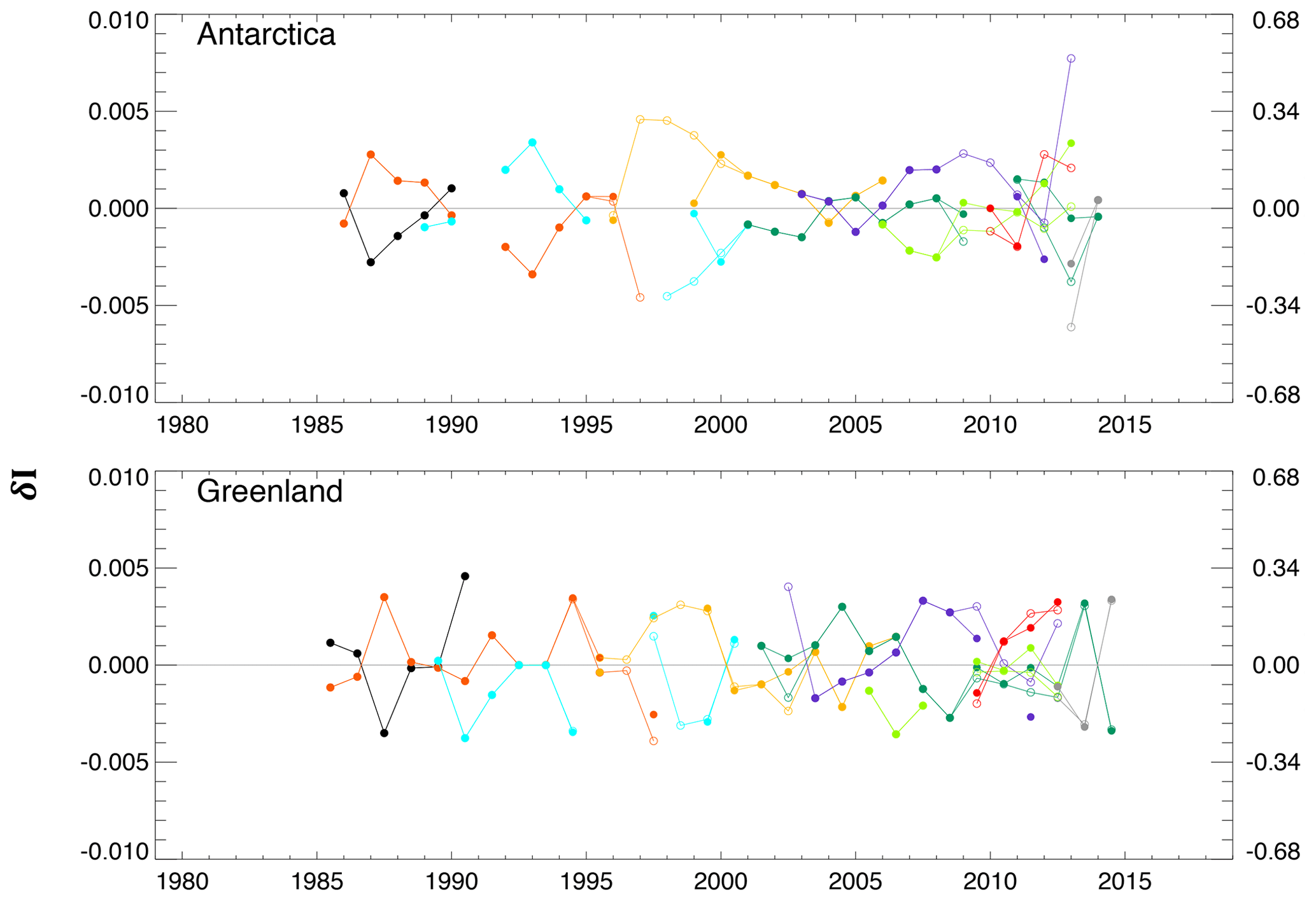
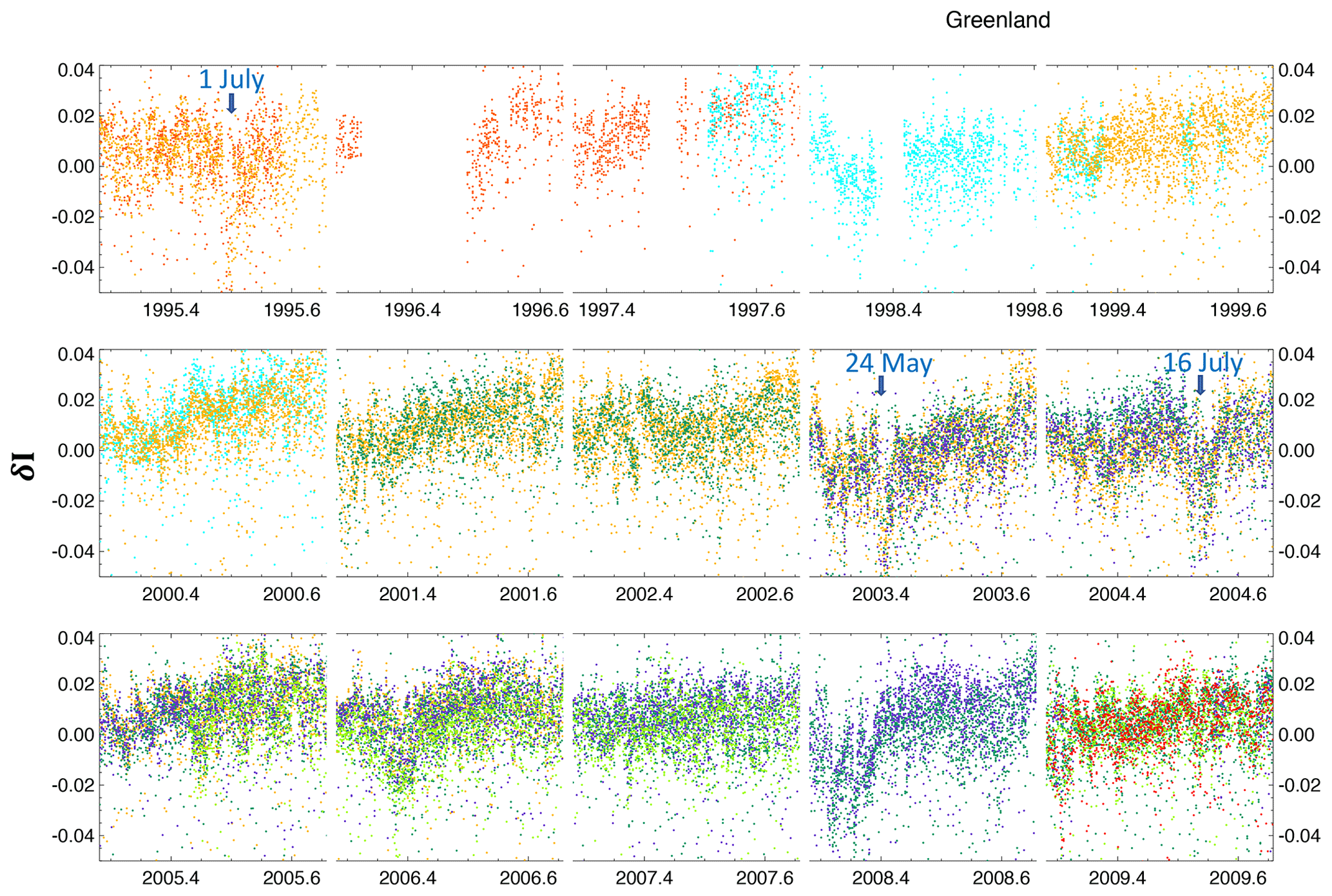
Figure 7Time series of empirically calibrated δI for all FOVs observed over Greenland for selected years. Blue arrows indicate estimated dates when CO from boreal forest fires reaches Greenland (see text). The color scheme is the same as the other figures.
The albedo of the Greenland Ice Sheet is of interest because it contributes to changes in the surface energy balance and surface melting. The variability of our UV δI record is consistent with the MODIS albedo data set. A recent study presents time series of the surface reflectance over the Greenland Ice Sheet from the Collection 5 (C5) and C6 MODIS data sets (Casey et al., 2017). While the older C5 set shows strong darkening of the ice sheet since 2000 (not shown), C6 has negligible trends that are not statistically significant. They report surface reflectance for the channel closest to our UV channel (MODIS Band 3, 459 nm) for dry snow conditions (locations with ice surface elevations >2000 m) and for wet snow conditions (elevations <2000 m). For easier comparison we have transcribed the data from their Fig. 4 onto our Fig. 4c. Many of the same episodic events in the MODIS C6 record that limit measurements to wet snow conditions (solid blue trace, Fig. 4c) are also seen by the UV instruments (Fig. 4b and c): darkening in the NH summer of 2003, 2010 and 2012. The 2012 darkening was likely driven by anomalous surface melting over Greenland. Satellite estimates of melt-day area from microwave brightness temperatures (Nghiem et al., 2012) and mass loss from the NASA GRACE instrument both suggest strong surface melting in 2012.
Surface or airborne light-absorbing aerosols that originate from boreal forest fires can explain some of the other reductions of UV δI over Greenland. The 1995 darkening episode is likely caused by forest fires in Canada. Using a trajectory model, Wotawa and Trainer (2000) estimate that CO emitted from the large fires in western Canada reach Greenland on 1 July (their Fig. 2). Using a similar technique, Stohl et al. (2006) estimate that CO from Alaskan and Canadian fires in 2004 reached Summit Greenland on about 16 July. Their Fig. 11 shows elevated levels of observed and trajectory-modeled CO from 16 July to 2 August. Finally, the global travels of smoke from the 2003 fires in southeastern Russia are documented by Damoah et al. (2004) using a trajectory model and MODIS satellite images. They estimate a 24 May arrival time over Greenland (their Fig. 2). A time series of daily values of UV δI over Greenland shows abrupt reductions by the SBUV instruments operating on those dates (Fig. 7). There are other dramatic darkening events, likely caused by either forest fire smoke or surface melting (e.g., 2006 and 2008), that we could not find in the literature.
While the shorter C6 record shows no apparent trend, our UV record shows a weak though statistically insignificant reduction in UV δI over Greenland: −0.05 (±0.06) decade−1 at locations with elevations >2000 m (Fig. 4b). Impurities in the snow as detected by in situ analysis are consistent with our observed trend. Polashenski et al. (2015) measured the concentrations of light-absorbing impurities (LAI) in 67 snow pits across the northwestern Greenland Ice Sheet in 2013 and 2014 and compared them with studies that analyzed snow from the past 6 decades. Increases in black carbon or dust concentrations relative to recent decades were small and corresponded to snow albedo reductions of at most 0.31, or ∼0.05 per decade, which is similar to our UV satellite estimate. The snow studies also record episodic events that darken the snow by 1 %–2 %, similar to the 1995, 2003 and 2004 darkening we see in the SBUV satellite record.
The East Antarctic Plateau is the preferred ice sheet for performing radiance calibration. Its very low temperatures and clear pristine conditions, except for the occasional volcanic eruption, all maintain a stable surface albedo with time. In contrast, the interior Greenland Ice Sheet is darkened every few years by airborne particles from boreal wildfires or from albedo changes caused by widespread surface melting. Since we are not doing an absolute calibration but a relative calibration (using NOAA-16 as a reference instrument), Greenland's albedo variations (∼2 %) test how well the SBUV instruments respond to changes in the albedo. Moreover, including it in our calibration analysis enables a characterization of instrument hysteresis errors mainly with Nimbus-7 over Antarctica. Once removed, it matters little whether both ice sheets or only Antarctica are used to determine the multiplicative gain coefficients (c1), the UV δI trends over both ice sheets are almost the same.
Intensities at the 340 nm wavelength channel observed by eight nadir-viewing SBUV satellite instruments and the OMPS scanning instrument are inter-calibrated over the Antarctic and Greenland ice sheets. The approach is to compare observed intensities that have been normalized by solar zenith angle. After the inter-calibration, we estimate a 2-sigma uncertainty of 0.35 % based on temporally overlapping sensors. Multiple instruments respond in unison to known darkening events that sometimes can be explained by volcanic aerosols, soot from boreal forest fires, or surface meltwater. These calibrated intensities will be used to derive a UV cloud albedo record over the tropics and midlatitudes since 1980.
Each instrument provides narrowband backscattered intensities close to but not exactly at 340 nm wavelength. For example, Nimbus-7, NOAA-9 and NOAA-14 have nominal center wavelengths of 339.90, 339.75, 340.05 nm and full width half maximum (FWHM) of 1.0, 1.132 and 1.132 nm, respectively. These seemingly small wavelength differences will change observed intensities by several tenths of a percent at high solar zenith angles. Using the VLIDORT radiative transfer model, we create a two-dimensional table of intensities at 0.1 nm wavelength resolution and at 10∘ SZA resolution. A Lambertian surface of 0.95 albedo is assumed. For each instrument we determine a simulated intensity Isim by convolving the instrument's FWHM across the center wavelength of the instrument. To account for the wavelength and FWHM difference between a non-reference instrument (e.g., Nimbus-7) and our reference instrument NOAA-16, we multiply the observed intensities from Nimbus-7 by I (θo)sim (. Note that the wavelength correction is dependent on solar zenith angle.
The SBUV intensities that were used in this study along with satellite geometry information are available on request.
CJW devised the calibration technique, PKB and DLW provided funding acquisition, and GJL and DEH helped with writing and editing.
The authors declare that they have no conflict of interest.
This work was supported by a NASA Making Earth System Data Records for Use in Research Environments (MEaSUREs) project and the NASA Long-term measurement of Ozone program. We appreciate the comments of the two reviewers.
This research has been supported by the NASA Long Term Measurement of Ozone (grant no. WBS 479717).
This paper was edited by Marcos Portabella and reviewed by two anonymous referees.
Casey, K. A., Polashenski, C. M., Chen, J., and Tedesco, M.: Impact of MODIS sensor calibration updates on Greenland Ice Sheet surface reflectance and albedo trends, The Cryosphere, 11, 1781–1795, https://doi.org/10.5194/tc-11-1781-2017, 2017.
Damoah, R., Spichtinger, N., Forster, C., James, P., Mattis, I., Wandinger, U., Beirle, S., Wagner, T., and Stohl, A.: Around the world in 17 days – hemispheric-scale transport of forest fire smoke from Russia in May 2003, Atmos. Chem. Phys., 4, 1311–1321, https://doi.org/10.5194/acp-4-1311-2004, 2004.
DeLand, M. T., Cebula, R. P., Huang, L.-K., Taylor, S. L., Stolarski, R. S., and McPeters, R. D.: Observations of “Hysteresis” in Backscattered Ultraviolet Ozone Data. J. Atmos. Ocean. Technol., 18, 914–924, https://doi.org/10.1175/1520-0426(2001)018<0914:OOHIBU>2.0.CO;2, 2001.
DeLand, M. T., Taylor, S. L., Huang, L. K., and Fisher, B. L.: Calibration of the SBUV version 8.6 ozone data product, Atmos. Meas. Tech., 5, 2951–2967, https://doi.org/10.5194/amt-5-2951-2012, 2012.
Herman, J., DeLand, M. T., Huang, L.-K., Labow, G., Larko, D., Lloyd, S. A., Mao, J., Qin, W., and Weaver, C.: A net decrease in the Earth's cloud, aerosol, and surface 340 nm reflectivity during the past 33 yr (1979–2011), Atmos. Chem. Phys., 13, 8505–8524, https://doi.org/10.5194/acp-13-8505-2013, 2013.
Huang, L.-K., Cebula, R. P., Taylor, S. L., DeLand, M. T., McPeters, R. D., and Stolarski, R. S.: Determination of NOAA-11 SBUV/2 radiance sensitivity drift based on measurements of polar ice cap radiance. Int. J. Remote Sens., 24, 305–314, https://doi.org/10.1080/01431160304978, 2003.
Jaross, G. and Warner, J.: Use of Antarctica for validating reflected solar radiation measured by satellite sensors, J. Geophys. Res., 113, D16S34, https://doi.org/10.1029/2007JD008835, 2008.
Labow, G., Herman, J. R., Huang, L.-K., Lloyd, S. A., DeLand, M. T., Qin, W., Mao, J., and Larko, D. E.: Diurnal variation of 340 nm Lambertian equivalent reflectivity due to clouds and aerosols over land and oceans, J. Geophys. Res., 116, D11202, https://doi.org/10.1029/2010JD014980, 2011.
Nghiem, S. V., Hall, D. K., Mote, T. L., Tedesco, M., Albert, M. R., Keegan, K., Shuman, C. A., DiGirolamo, N. E., and Neumann, G.: The extreme melt across the Greenland Ice Sheet in 2012. Geophys. Res. Lett., 39, L20502, https://doi.org/10.1029/2012GL053611, 2012.
Polashenski, C. M., Dibb, J. E., Flanner, M. G., Chen, J. Y., Courville, Z. R., Lai, A. M., Schauer, J. J., Shafer, M. M., and Bergin, M.: Neither dust nor black carbon causing apparent albedo decline in Greenland's dry snow zone: Implications for MODIS C5 surface reflectance, Geophys. Res. Lett., 42, 9319–9327, https://doi.org/10.1002/2015GL065912, 2015.
Seftor, C. J., Jaross G., Kowitt M., Haken, M., Li, J., and Flynn, L. E.: Postlaunch performance of the Suomi National Polar- orbiting Partnership Ozone Mapping and Profiler Suite (OMPS) nadir sensors, J. Geophys. Res.-Atmos., 119, 4413–4428, https://doi.org/10.1002/2013JD020472, 2014.
Spurr, R. J. D.: VLIDORT: A linearized pseudo-spherical vector discrete ordinate radiative transfer code for forward model and retrieval studies in multilayer multiple scattering media, J. Quant. Spectrosc. Rad. Transf., 102, 316–342, https://doi.org/10.1016/j.jqsrt.2006.05.005, 2006.
Stohl, A., Andrews, E., Burkhart, J. F., Forster, C., Herber, A., Hoch, S. W., Kowal, D., Lunder, C., Mefford, T., Ogren, J. A., Sharma, S., Spichtinger, N., Stebel, K., Stone, R., Ström, J., Tørseth, K., Wehrli, C., and Yttri, K. E.: Pan-Arctic enhancements of light absorbing aerosol concentrations due to North American boreal forest fires during summer 2004, J. Geophys. Res., 111, D22214, https://doi.org/10.1029/2006JD007216, 2006.
Weaver, C. J., Herman, J. R., Labow, G. J., Larko, D., and Huang, L.-K.: Shortwave TOA Cloud Radiative Forcing Derived from a Long-Term (1980–Present) Record of Satellite UV Reflectivity and CERES Measurements, J. Climate, 28, 9473–9488, https://doi.org/10.1175/JCLI-D-14-00551.1, 2015.
Weaver, C. J., Wu, D. L., Bhartia, P. K., Labow, G. J., and Haffner, D. P.: A Long-Term Cloud Albedo Data Record Since 1980 from UV Satellite Sensors, Remote Sens., 12, 1982, https://doi.org/10.3390/rs12121982, 2020.
Wotawa, G. and Trainer, M.: The influence of Canadian forest fires on pollutant concentrations in the United States, Science, 288, 324–328, 2000.
- Abstract
- Motivation
- Previous calibration of UV satellite records
- Empirically based inter-calibration
- Adjusting the intensities
- Greenland Ice Sheet
- Discussion/summary
- Appendix A: Accounting for small wavelength differences
- Data availability
- Author contributions
- Competing interests
- Acknowledgements
- Financial support
- Review statement
- References