The quantification of NO_x and SO₂ point source emission flux errors of mobile differential optical absorption spectroscopy on the basis of the Gaussian dispersion model: a simulation study

Mobile differential optical absorption spectroscopy (mobile DOAS) has become an important tool for the quantification of emission sources, including point sources (e.g., individual power plants) and area emitters (e.g., entire cities). In this study, we focused on the error budget of mobile DOAS measurements from point sources, and we also offered recommendations for the optimum settings of such measurements via a simulation with a modified Gaussian plume model. Following the analysis, we conclude that (1) the proper sampling resolution should be between 5 and 50 m. (2) When measuring far from the source, undetectable flux (measured slant column densities (SCDs) are under the detection limit) resulting from wind dispersion is the main error source. The threshold for the undetectable flux can be lowered by larger integration time. When measuring close to the source, low sampling frequency results in large errors, and wind field uncertainty becomes the main error source of SO₂ flux (for NO_x this error also increases, but other error sources dominate). More measurement times can lower the flux error that results from wind field uncertainty. The proper wind speed for mobile DOAS measurements is between 1 and 4 m s⁻¹. (3) The remaining errors by [NO_x] ∕ [NO₂] ratio correction can be significant when measuring very close. To minimize the [NO_x] ∕ [NO₂] ratio correction error, we recommend minimum distances from the source, at which 5 % of the NO₂ maximum reaction rate is reached and thus NO_x steady state can be assumed. (4) Our study suggests that emission rates < 30 g s⁻¹ for NO_x and < 50 g s⁻¹ for SO₂ are not recommended for mobile DOAS measurements.

Based on the model simulations, our study indicates that mobile DOAS measurements are a very well-suited tool to quantify point source emissions. The results of our sensitivity studies are important to make optimum use of such measurements.

1 Introduction

Nitrogen oxides (NO_x = NO + NO₂) and sulfur dioxide (SO₂), poisonous and harmful trace gases in the atmosphere, are critical participants in tropospheric chemical reactions (Seinfeld and Pandis, 1998; Beirle et al., 2003). NO_x and SO₂ are emitted into the atmosphere via natural and anthropogenic emissions, especially from traffic and industries. In recent years, China has experienced large areas of haze pollution, which have drawn worldwide scrutiny due to their NO_x, SO₂, and volatile organic compound content, although strict policies designed to control the emission of pollution gases have been implemented (Richter, et al., 2005; Ding et al., 2015; Jin et al., 2016; Zhang et al., 2019, 2020). It is of great significance to study gas emission pollution both qualitatively and quantitatively.

Differential optical absorption spectroscopy (DOAS) is a technique developed in the 1970s that focuses on the telemetering of atmospheric gases, particularly trace gases (Platt and Stutz, 2008). After years of research, various types of DOAS technology have been comprehensively developed, including LP-DOAS, MAX-DOAS, and mobile DOAS.

Mobile DOAS technology was originally used to measure volcanic SO₂ emissions (Bobrowski et al., 2003; Edmonds et al., 2003; Galle et al., 2003), and it was then developed to measure the NO₂ and SO₂ emission fluxes from industrial parks (Johansson et al., 2008). In 2008, Mattias Johansson used a mobile mini-DOAS device to quantify the total emission of air pollutants from Beijing and evaluated the measurement error, mainly in terms of the uncertainties in the wind field, experimental setup, sunlight scattering in the lower atmosphere, and DOAS fit error. During the MCMA 2006 field campaign, Rivera et al. (2009) used a mobile mini-DOAS instrument to measure the NO₂ and SO₂ emissions of the Tula industrial complex in Mexico and also estimated the flux error. In Ibrahim et al. (2010), Wagner et al. (2010), and Shaiganfar et al. (2011, 2017), air mass factor (AMF), sampling resolution, NO_x chemical reactions, and atmospheric lifetime were introduced in order to analyze the emission flux error. The analysis of emission flux error sources has gradually come to focus on the wind field uncertainty, sampling resolution measurement error (GPS error), slant column density (SCD) fit error, AMF error, and other error sources. The aforementioned studies primarily concentrated on regional/industry park emission fluxes, as opposed to point sources.

Different from regional/industry park measuring, point source emission flux can be measured in diverse ways, with different measuring distances, varying sampling resolutions, and so on. Therefore, the error sources and influence factors affecting the flux measurements are different. In order to investigate the impact of these factors and thereby recommend optimum settings for point source flux measuring using mobile DOAS, we performed an in-depth study on the effects of error sources and influence factors on point source emission flux measuring.

There are innate deficiencies in the experimental method used to analyze the emission flux error since there are so many scenarios that need to be verified, and the various factors cannot be well controlled during experiments. Therefore, a convenient way to assist the analysis is sorely needed. In the absence of precise requirements, the simulation method is a good alternative for facilitating the analysis of mobile DOAS emission flux error, given its convenience and feasibility.

Using a model based on Gaussian plume dispersion and the mobile DOAS emission flux measurement method, we here performed a simulation to study the measurement of NO_x and SO₂ point source emission flux.

This paper is organized as follows: in Sect. 2, the methodological framework is presented. In Sect. 3, the parameters used to drive the simulation are delineated. Section 4 describes the simulation performance and data analysis, Sect. 5 presents our conclusions, and the Appendix displays the overall simulation results.

2 Methodology and forward model

2.1 Overview of methodology

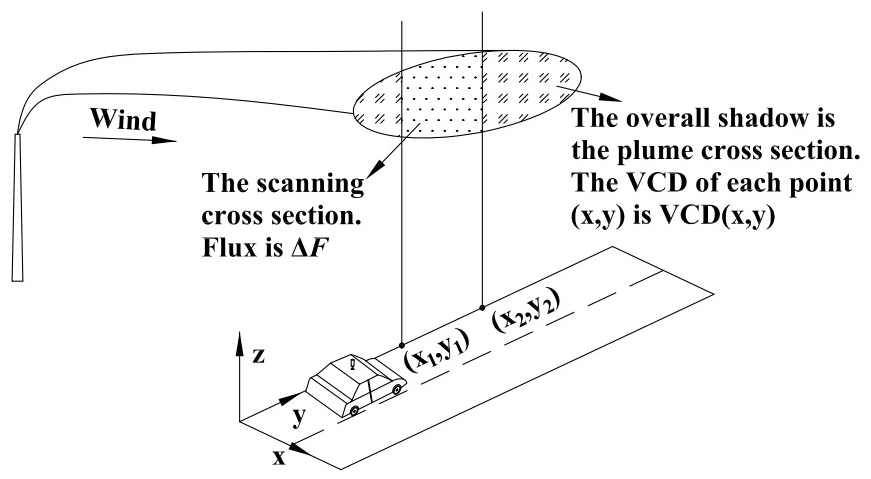
The NO_x and SO₂ emission flux of the point source can be well measured by the mobile DOAS. The equation for calculating the emission flux in the discrete form is expressed as

$$\begin{array}{}\text{(1)}& F=\sum _j{\mathrm{VCD}}_j\cdot \overrightarrow{u_j}\cdot \overrightarrow{n_j}\cdot s_j,\end{array}$$

where F is the emission flux, ${\mathrm{VCD}}_j={\mathrm{SCD}}_j/{\mathrm{AMF}}_j$ , SCD_j is the SCD for mobile DOAS measurements along the measurement route, AMF_j is the air mass factor, $\overrightarrow{u_j}$ is the wind field, $\overrightarrow{n_j}$ is the vector pointing to the right of the driving direction and parallel to the Earth's surface, and s_j is the sampling resolution. For an isolated point source, the mobile DOAS can measure underneath the plume in the downwind direction to quantify the emission flux.

Figure 1 Schematic diagram of the modeled mobile DOAS measurement underneath the plume.

Since individual experiments take place in complex and variable scenarios, in order to investigate the error sources and influence factors that impact the flux measurement error, typical mobile DOAS measurements of the NO_x and SO₂ emission fluxes were modeled with the following assumptions.

1. NO_x and SO₂ gas continuously exhaust from an isolated and elevated point source at the position (0, 0, 235 m). The plume rises approximately 15 m.

2. The plume is diluted by the wind along the wind direction (x axis). The random movement of air parcels also dilutes the plume in the cross section and in the vertical directions (y axis and z axis).

3. The topography around the point source is flat and the background concentration of the pollutants is regarded as zero. In the case of non-negligible background concentrations, the vertical column densities (VCDs) in the plume have to be calculated as the difference to the background.

4. Air turbulence is constant in space and time.

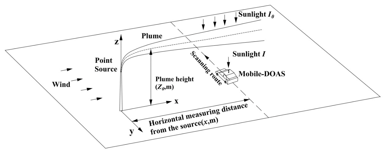
5. A zenith-sky mobile DOAS measures the gas underneath the plume in the y direction at around noon (see Fig. 1). Spectra, GPS data, and wind profiles are available for individual measurements.

6. The sunlight radiance received by the mobile DOAS instrument is stable.

Figure 1 presents the schematic diagram of the modeled mobile DOAS measurement of a point source.

Figure 2 Forward model of mobile DOAS measurements and error analysis.

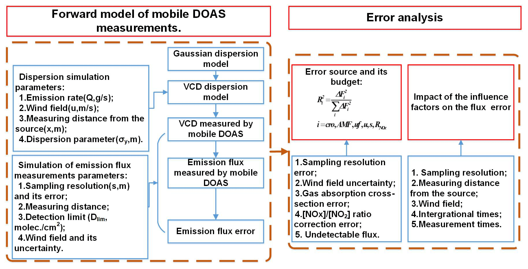
Based on the performance of typical mobile DOAS measurements, a forward model of flux calculations was generated and error analysis performed according to the forward model, as shown in Fig. 2.

The forward model of mobile DOAS measurements can be divided into two steps.

1. Dispersion simulation. In this step, a dispersion model is established to generate the vertical column densities (VCDs) measured by the mobile DOAS in the modeled typical measurement.

2. Simulation of emission flux measurement. After the VCD sequence along the measurement route is generated, the next step is calculating the emission flux and the emission flux error.

Error analysis concentrates on the error sources and their budget and the influence factors that affect the emission flux error.

The emission flux and VCD retrieval calculation model can be directly introduced into our forward model, as it has in previous studies. However, some questions concerning the forward model still exist:

1. Is the existing dispersion model suitable for the mobile DOAS measurement depicted in Fig. 1?

2. How can VCDs be simulated in the same way as mobile DOAS measurements in theory?

3. Mobile DOAS can measure NO₂ instead of NO_x. How can the NO ↔ NO₂ conversion be added to the existing dispersion model in terms of this simulation?

These questions will be explored in Sect. 2.2–2.6.

2.2 Description of Gaussian dispersion model

2.2.1 Steady-state Gaussian dispersion model

An appropriate air dispersion model needed to be chosen for generating the forward model of mobile DOAS measurements. Since the concentrations of pollutants at individual points in the air parcels of the plume under the assumptions we have made can be calculated based on the Gaussian dispersion model (Arystanbekova, 2004; Lushi and Stockie, 2010; de Visscher, 2014), we applied the Gaussian dispersion model in this study. The plume, as reflected by the surface due to the ground boundary effect and the dispersion model, can be expressed as Eq. (2).

$$\begin{array}{}\text{(2)}& \begin{array}{rl}c(x,y,z)& ={\displaystyle \frac{DQ}{\mathrm{2}\mathit{\pi }u{\mathit{\sigma }}_y{\mathit{\sigma }}_z}}\exp \left(-{\displaystyle \frac{y^{\mathrm{2}}}{\mathrm{2}{\mathit{\sigma }}_y^{\mathrm{2}}}}\right)\\ & \cdot \left\{\exp \left[-{\displaystyle \frac{(z+H{)}^{\mathrm{2}}}{\mathrm{2}{\mathit{\sigma }}_z^{\mathrm{2}}}}\right]+\exp \left[-{\displaystyle \frac{(z-H{)}^{\mathrm{2}}}{\mathrm{2}{\mathit{\sigma }}_z^{\mathrm{2}}}}\right]\right\},\end{array}\end{array}$$

where Q is the emission rate (g s⁻¹); u is the wind speed (m s⁻¹) and the wind direction is along the x direction; σ_y (m) is the dispersion parameter in the y direction; σ_z (m) is the dispersion parameter in the z direction, with σ_y and σ_z dependent on x; and H is the plume height (m). $D=\exp (-\mathit{\phi }\frac{x}{u}$) is the decay term, mainly consisting of the chemical reactions and deposits; φ is the decay coefficient; and $\mathit{\phi }=\frac{\ln \mathrm{2}}{T_{\mathrm{1}/\mathrm{2}}}$, in which T_1∕2 is the pollutant half-life in seconds.

The dispersion parameters are determined by the atmospheric stability. The classification of atmospheric stability, which was created by Pasquill and Gifford and is widely used, sorts atmospheric stability into six classes ranging from A to F (de Visscher, 2014). We only considered the classifications under strong solar radiation (see Table 1) in this study.

Table 1 Pasquill–Gifford atmospheric stability classifications.

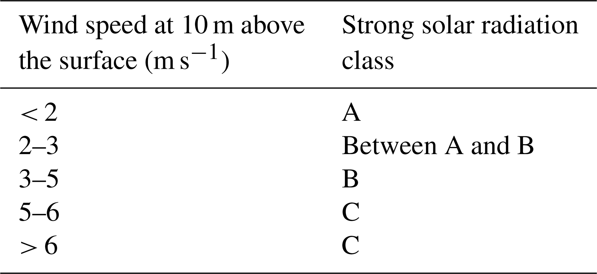
A: very unstable; B: moderately unstable; C: slightly unstable.

Based on the atmospheric stability class and the terrain type surrounding the emission point, the parameters σ_y and σ_z can be calculated. Since we assumed the surrounding area to be flat, rural terrain, the σ_y and σ_z parameters could be calculated using the formulas of Briggs (1973), listed in Table 2.

Table 2 Rural area air dispersion parameters (Briggs, 1973).

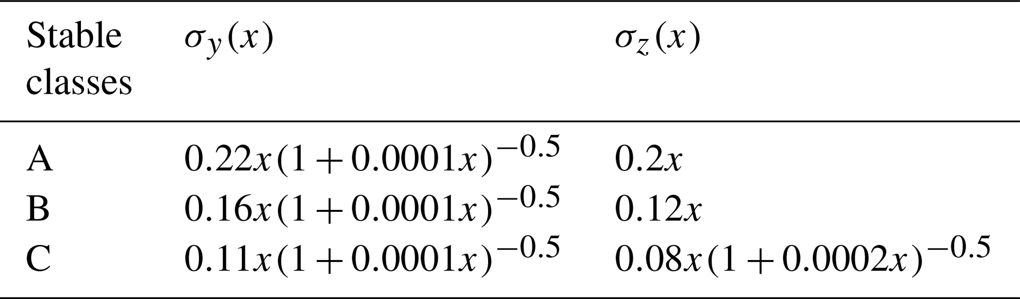
In which x is the horizontal distance from the source, in meters.

It should be noted that Briggs's equations are only suitable under the condition of x lower than 10 km. The dispersion in the wind direction is negligible in comparison with the advection when the wind speed is high, or for weak turbulence (de Visscher, 2014). In addition, the model accuracy significantly decreases in the case of wind speeds < 1 m s⁻¹. The critical wind speed for the Gaussian dispersion model is about 1.2 m s⁻¹ (de Visscher, 2014). For high wind speed, the effect of undetectable flux becomes very important (see e.g., results in Fig. 8). Thus for the general cases considered here measurements under high wind speed are not recommended. Only for very high emissions and close to the source (< 1 km) might measurements for high wind speeds be meaningful, but such situations might be rare. Since our study focuses on the general cases, we limit it to wind speeds < 8 m s⁻¹, because in the range up to 8 m s⁻¹ the general dependencies become obvious. Therefore, the wind speed range in our simulation is between 1.2 and 8 m s⁻¹. The distance in our simulation is within 10 km.

2.2.2 NO_x dispersion

Equation (2) is suitable for SO₂ dispersion, while for NO_x, mobile DOAS can only measure NO₂ effectively. Hence, Eq. (2) should be adjusted for NO₂ dispersion based on NO_x atmospheric chemical reactions. In this study, we did not take volatile organic compounds (VOCs) into consideration; thus, a NO_x balance would not be broken. Moreover, we assume that no NO_x is presented in the ambient air and no O₃ is consumed in the reaction with NO. In most cases, both assumptions are reasonable, especially as long as the background NO_x concentration has no strong spatial–temporal variation. However, for very high emission rates, the assumption that no O₃ is consumed in the reaction with NO might be violated (a simple criterion to identify such cases might be to check whether the NO_x mixing ratios are higher than the ambient O₃ mixing ratios). If this is the case, the conversion of NO to NO₂ will be delayed. The typical reactions of NO, NO₂, O₃, and O₂ in the air parcels of the plume are

$$\begin{array}{}\text{(R1)}& {\displaystyle }{\mathrm{NO}}_{\mathrm{2}}+h\mathit{\nu }\to \mathrm{NO}+\mathrm{O}{(}^{\mathrm{3}}\mathrm{P}),\text{(R2)}& {\displaystyle }{\mathrm{O}}_{\mathrm{2}}+\mathrm{O}{(}^{\mathrm{3}}\mathrm{P})\to {\mathrm{O}}_{\mathrm{3}},\text{(R3)}& {\displaystyle }\mathrm{NO}+{\mathrm{O}}_{\mathrm{3}}\to {\mathrm{NO}}_{\mathrm{2}}+{\mathrm{O}}_{\mathrm{2}}.\end{array}$$

The reaction rates of Reactions (R1)–(R3) form a cyclic reaction. The reaction rate of NO₂ is

$$\begin{array}{}\text{(3)}& r_{{\mathrm{NO}}_{\mathrm{2}}}=-j_{\mathrm{3}}\left[{\mathrm{NO}}_{\mathrm{2}}\right]+k_{\mathrm{5}}\left[\mathrm{NO}\right][{\mathrm{O}}_{\mathrm{3}}{]}_t,\end{array}$$

where [gas] stands for the concentration of a particular gas, [O₃]_t is the O₃ concentration in the air parcels of the plume at time t, and t is the time period after NO_x is emitted into the atmosphere. We assumed that at the beginning there is no O₃ in the air parcels of the plume. During the mixing with outside air, the O₃ concentration within the air parcels increases. For simplicity, we assumed that the O₃ concentration is the same everywhere in a transect of the plume. j₃ is the NO₂ photochemical rate constant, equal to approximately 8 $\times {\mathrm{10}}^{-\mathrm{3}}$ s⁻¹, and k₅ is the rate constant of Reaction (R3), equal to approximately 1.8 $\times {\mathrm{10}}^{-\mathrm{14}}$ cm³ molec.⁻¹ s⁻¹ (de Visscher, 2014). It should be noted that these rates are for a temperature of 25 ^∘C. Fortunately, they are not sensitive to temperature, so temperature sensitivity did not need to be considered.

The [NO_x] ∕ [NO₂] ratio depends on the mixing ratio of O₃ inside the plume. The mixing ratio of O₃ within the air parcel of the plume can then be estimated as

$$\begin{array}{}\text{(4)}& \begin{array}{rl}[{\mathrm{O}}_{\mathrm{3}}{]}_t& =\left[{\mathrm{O}}_{\mathrm{3}}\right]{\displaystyle \frac{V_t-V_{\mathrm{0}}}{V_t}}=\left[{\mathrm{O}}_{\mathrm{3}}\right]{\displaystyle \frac{S_t\mathrm{\Delta }t-S_{\mathrm{0}}\mathrm{\Delta }t}{S_t\mathrm{\Delta }t}}\\ & =\left[{\mathrm{O}}_{\mathrm{3}}\right]\left(\mathrm{1}-{\displaystyle \frac{S_{\mathrm{0}}}{S_t}}\right),\end{array}\end{array}$$

where V₀ is the initial gas volume of the plume and S₀ is the initial gas cross section of the plume, while V_t is the gas volume of the plume at time t and S_t is the gas cross section of the plume in the atmosphere at time t. Here, [O₃] is the ambient O₃ concentration. The NO₂ concentration inside the plume at time t is given by

$$\begin{array}{}\text{(5)}& [{\mathrm{NO}}_{\mathrm{2}}{]}_t=\underset{\mathrm{0}}{\overset{t}{\int }}{r}_{{\mathrm{NO}}_{\mathrm{2}}}\mathrm{d}t.\end{array}$$

Since the NO₂ initial concentration was very low, we assumed the NO₂ initial concentration [NO₂]₀=0. Consequently, [NO_x]_t=[NO]₀ (with no decay).

The [NO_x] ∕ [NO₂] ratio at time t is

$$\begin{array}{}\text{(6)}& R_{{\mathrm{NO}}_x}={\displaystyle \frac{[{\mathrm{NO}}_x{]}_t}{[{\mathrm{NO}}_{\mathrm{2}}{]}_t}}.\end{array}$$

Different from SO₂, the number of NO_x molecules is conserved, as opposed to their mass. The NO_x dispersion model should thus be expressed as

$$\begin{array}{}\text{(7)}& \begin{array}{rl}{c}_{{\mathrm{NO}}_x}& (x,y,z)={\displaystyle \frac{D{Q}_{m_{{\mathrm{NO}}_x}}}{\mathrm{2}\mathit{\pi }u{\mathit{\sigma }}_y{\mathit{\sigma }}_z}}\exp \left(-{\displaystyle \frac{y^{\mathrm{2}}}{\mathrm{2}{\mathit{\sigma }}_y^{\mathrm{2}}}}\right)\\ & \cdot \left\{\exp \left[-{\displaystyle \frac{(z+H{)}^{\mathrm{2}}}{\mathrm{2}{\mathit{\sigma }}_z^{\mathrm{2}}}}\right]+\exp \left[-{\displaystyle \frac{(z-H{)}^{\mathrm{2}}}{\mathrm{2}{\mathit{\sigma }}_z^{\mathrm{2}}}}\right]\right\},\end{array}\end{array}$$

where $Q_{m_{{\mathrm{NO}}_x}}=\frac{Q\cdot \mathrm{NA}}{m_{{\mathrm{NO}}_x}}$. $m_{{\mathrm{NO}}_x}$ is the mean molar mass of the initial NO_x, and NA is Avogadro's constant of 6.02 ×10²³ molec. mol⁻¹. Substituting Eq. (6) into Eq. 7), the NO₂ dispersion model can then be expressed as

$$\begin{array}{}\text{(8)}& c_{{\mathrm{NO}}_{\mathrm{2}}}(x,y,z)={\displaystyle \frac{c_{{\mathrm{NO}}_x}(x,y,z)}{R_{{\mathrm{NO}}_x}}}.\end{array}$$

2.3 VCD dispersion model

As discussed above, mobile DOAS retrieves the VCD, while results of the dispersion model are point concentrations of the air parcels. Based on the definition of VCD, we integrate the concentration along the vertical direction, i.e., the z direction from the ground to the upper troposphere, as in

$$\begin{array}{}\text{(9)}& \begin{array}{rl}\mathrm{VCD}& (x,y)=\underset{\mathrm{0}}{\overset{+\mathrm{\infty }}{\int }}Dc(x,y,z)\mathrm{d}z={\displaystyle \frac{DQ}{\sqrt{\mathrm{2}\mathit{\pi }}u{\mathit{\sigma }}_y{\mathit{\sigma }}_z}}\\ & \underset{\mathrm{0}}{\overset{+\mathrm{\infty }}{\int }}\left\{\exp \left[-{\displaystyle \frac{(z+H{)}^{\mathrm{2}}}{\mathrm{2}{\mathit{\sigma }}_z^{\mathrm{2}}}}\right]+\exp \left[-{\displaystyle \frac{(z-H{)}^{\mathrm{2}}}{\mathrm{2}{\mathit{\sigma }}_z^{\mathrm{2}}}}\right]\right\}\mathrm{d}z\\ & ={\displaystyle \frac{DQ}{\sqrt{\mathrm{2}\mathit{\pi }}u{\mathit{\sigma }}_y}}\exp \left(-{\displaystyle \frac{y^{\mathrm{2}}}{\mathrm{2}{\mathit{\sigma }}_y^{\mathrm{2}}}}\right).\end{array}\end{array}$$

Equation (9) is suitable for SO₂. For NO_x, the VCD dispersion is

$$\begin{array}{}\text{(10)}& {\mathrm{VCD}}_{{\mathrm{NO}}_x}(x,y)={\displaystyle \frac{D{Q}_{m_{{\mathrm{NO}}_x}}}{\sqrt{\mathrm{2}\mathit{\pi }}u{\mathit{\sigma }}_y}}\exp \left(-{\displaystyle \frac{y^{\mathrm{2}}}{\mathrm{2}{\mathit{\sigma }}_y^{\mathrm{2}}}}\right).\end{array}$$

The NO₂ VCD dispersion model is

$$\begin{array}{}\text{(11)}& {\mathrm{VCD}}_{{\mathrm{NO}}_{\mathrm{2}}}(x,y)={\displaystyle \frac{{\mathrm{VCD}}_{{\mathrm{NO}}_x}(x,y)}{R_{{\mathrm{NO}}_x}}}.\end{array}$$

Since NO_x disperses along the wind direction and $R_{{\mathrm{NO}}_x}$ is a function of t, this means that $R_{{\mathrm{NO}}_x}$ also varies with distance. The detailed relationship between the distance and $R_{{\mathrm{NO}}_x}$ will be discussed in Sect. 4.4. Equations (9)–(11) lay the mathematical foundation of the VCD distribution model for mobile DOAS measuring.

2.4 VCD measured by mobile DOAS

As shown in Fig. 3, the flux of the plume cross section can be calculated using the following equation:

$$\begin{array}{}\text{(12)}& \mathrm{\Delta }{F}_j=u\cdot \underset{l}{\int }\mathrm{VCD}(x,y)\mathrm{d}s.\end{array}$$

ΔF_j is the flux along the measurement route l in theory. For mobile DOAS measurement, ΔF_j should be given by Eq. (13):

$$\begin{array}{}\text{(13)}& \mathrm{\Delta }{F}_j={\mathrm{VCD}}_j\cdot \mathrm{u}\cdot s_j,\end{array}$$

where s_j is the distance between two measuring points and VCD_j can be derived from the spectrum of measurement j. Based on Eqs. (12) and (13), VCD_j can be expressed by Eq. (14).

$$\begin{array}{}\text{(14)}& {\mathrm{VCD}}_j={\displaystyle \frac{\mathrm{1}}{s}}\underset{l}{\int }\mathrm{VCD}(x,y)\mathrm{d}s\end{array}$$

Equation (14) indicates that the VCD_j derived from individual mobile DOAS measurements is the average of VCD(x,y) along the measurement route. The discretization of the VCD can significantly affect the emission flux error and will be discussed in Sect. 4.1.

Figure 3 Model of VCD measured by mobile DOAS.

2.5 Description of emission flux measured by mobile DOAS

Since the SO₂ lifetime scale is longer than the dispersion timescale, a decay correction is not needed for SO₂, but for NO_x it can be necessary. For the SO₂ emission flux, Eq. (1) is used, while the NO_x emission flux is

$$\begin{array}{}\text{(15)}& F_{{\mathrm{NO}}_x}={\displaystyle \frac{R_{{\mathrm{NO}}_x}}{D}}{F}_{{\mathrm{NO}}_{\mathrm{2}}}.\end{array}$$

In fact, the decay correction for NO_x should be applied for cases with low wind speeds, while the effect for high wind speeds is very small.

2.6 Measurement errors of emission flux

Emission flux measurement errors not only arise from measurement errors but also depend on other factors, such as wind speed, measuring distance, [NO_x] ∕ [NO₂] ratio, and the sampling resolution.

Since the VCD is inversely proportional to the wind speed (Eqs. 9 and 10), the higher the wind speed is, the lower the VCD. This means more measurements at the edge of plume would be under the detection limit at higher wind speeds, causing more undetectable flux. The VCD is also inversely proportional to measuring distance (Eqs. 9 and 10). This means that the undetectable flux increases with measuring distance. Since the [NO_x] ∕ [NO₂] ratio depends on the measuring distance (see Fig. 10), a large [NO_x] ∕ [NO₂] ratio correction error occurs when the measuring distance is small. Finally, the sampling error can be reduced with improved sampling resolution.

The emission flux measurement errors by mobile DOAS have several sources: SCD fit errors, AMF errors, wind field uncertainties, and sampling resolution measurement errors (Johansson et al., 2008, 2009; Wagner et al., 2010; Ibrahim et al., 2010; Shaiganfar et al., 2011, 2017; Rivera, et al., 2009).

The uncertainty of the derived SCD from the DOAS fit has a random and systematic part. For the random part it can be assumed that in general it cancels out (in combination with the sampling resolution error it can have a very small contribution). Thus, its direct effect on the total flux error is neglected in the following. However, from the fit error the detection limit is also estimated. For SCDs below the mobile DOAS detection limit, undetectable SCDs result in undetectable flux, and therefore the fit error indirectly contributes to the total flux error.

The systematic part of the SCD error caused by the uncertainty of the trace gas absorption cross section is independent from the SCD fit error and is therefore included as an additional term in the total flux error calculation.

We assume that these errors are random, have a Gaussian distribution, and are independent of each other. Then the total relative error of the emission flux is given by

$$\begin{array}{}\text{(16)}& \begin{array}{rl}{E}_{\mathrm{total}}& ={\displaystyle \frac{F_{\mathrm{err}}}{D\cdot Q}}\times \mathrm{100}\mathit{\%}\\ & ={\displaystyle \frac{\sqrt{\mathrm{\Delta }{F}_{\mathrm{cro}}^{\mathrm{2}}+\mathrm{\Delta }{F}_{\mathrm{uf}}^{\mathrm{2}}+\mathrm{\Delta }{F}_{\mathrm{AMF}}^{\mathrm{2}}+\mathrm{\Delta }{F}_{\mathrm{u}}^{\mathrm{2}}+\mathrm{\Delta }{F}_{\mathrm{s}}^{\mathrm{2}}}}{D\cdot Q}}\\ & \times \mathrm{100}\mathit{\%},\end{array}\end{array}$$

where F_err is the total flux error, ΔF_cro is the flux error introduced by gas absorption cross-section error, ΔF_uf is the undetectable flux, ΔF_AMF is the flux error introduced by AMF errors, and ΔF_u is the flux error introduced by wind speed uncertainty. The wind direction uncertainties play a smaller role in point source flux measuring error (and can be derived from geometry); thus the uncertainties caused by the wind field are dominated by the wind speed uncertainties. The error term of the wind direction uncertainty is therefore removed. ΔF_s is the emission flux error introduced by sampling resolution measurement error and it can be neglected (see Sect. 4.1).

Equation (16) is appropriate for SO₂. With regard to NO_x, the NO_x flux error is also introduced by the decay correction and the [NO_x] ∕ [NO₂] ratio correction error. Hence, the NO_x flux relative error is

$$\begin{array}{}\text{(17)}& \begin{array}{rl}{E}_{{\mathrm{NO}}_x}& ={\displaystyle \frac{F_{\mathrm{err}}}{D\cdot Q}}\times \mathrm{100}\mathit{\%}\\ & ={\displaystyle \frac{\sqrt{\mathrm{\Delta }{F}_{R_{{\mathrm{NO}}_x}}^{\mathrm{2}}+\mathrm{\Delta }{F}_{\mathrm{cro}}^{\mathrm{2}}+\mathrm{\Delta }{F}_{\mathrm{uf}}^{\mathrm{2}}+\mathrm{\Delta }{F}_{\mathrm{AMF}}^{\mathrm{2}}+\mathrm{\Delta }{F}_{\mathrm{u}}^{\mathrm{2}}+\mathrm{\Delta }{F}_{\mathrm{s}}^{\mathrm{2}}}}{D\cdot Q}}\\ & \times \mathrm{100}\mathit{\%},\end{array}\end{array}$$

where ΔF_D is the flux error due to decay correction, and $\mathrm{\Delta }{F}_{R_{{\mathrm{NO}}_x}}$ is the flux error due to [NO_x] ∕ [NO₂] ratio correction.

In order to quantify the contributions and budget of individual error sources, the ratios are calculated as Eq. (18):

$$\begin{array}{}\text{(18)}& R_i^{\mathrm{2}}={\displaystyle \frac{\mathrm{\Delta }{F}_i^{\mathrm{2}}}{F_{\mathrm{err}}^{\mathrm{2}}}},\end{array}$$

where i represents the individual error sources. Note that $\sum _i{R}_i^{\mathrm{2}}=\mathrm{1}$.

3 Parameter assumption and numerical simulation

In Sect. 2, the forward model for mobile DOAS measurements of emission flux was established. In this section, reasonable values of the parameters in the forward model are discussed and prepared in order to drive the forward model.

For most factories, including power plants, the emission rates of NO_x and SO₂ are different. Since a higher emission rate is an ideal condition for mobile DOAS measurements, higher emissions could be outside the scope of our study. Therefore, the emission rate that we simulated was < 200 g s⁻¹, and we set the Q value within this range. Since the Gaussian dispersion model is appropriate for moderate wind speed and scale, the wind speed was set to range from 1.2 to 8 m s⁻¹ and the dispersion distance was approximately 0–10 km. Given the car speed and mobile DOAS spectrometer integration times t_int, the sampling resolution was set from 5 to 500 m. The NO_x mean daytime lifetime is approximately 5 h ± 1 h (Spicer, 1982), while the SO₂ daytime lifetime is more than 1 d (Beirle et al., 2014). Compared with the dispersion timescale, the SO₂ daytime lifetime uncertainty could be neglected. When time approaches infinity, the NO_x reaction steady state could be determined by ambient [O₃] according to Eq. (5). We here assumed a typical [O₃] value of 1.389 ×10¹² molec. cm⁻³; thus the steady-state [NO_x] ∕ [NO₂] ratio is 1.32. The [NO_x] ∕ [NO₂] ratio inside the air parcel of the plume varying with the distance could be determined by Eqs. (5)–(8).

The SCD error can mainly be attributed to the DOAS fitting error of the SCD and the trace gas absorption cross-section error. Previous studies have indicated that the typical fit errors of NO₂ and SO₂ SCDs are ± (1–4) ×10¹⁵ and ± (1–6) ×10¹⁵ molec. cm⁻², respectively (Wagner et al., 2011; Wang et al., 2014; Wu et al., 2018; Davis et al., 2019). Thus in this study, we set the fit error of NO₂ and SO₂ to be ± 2.5 ×10¹⁵ and ± 4 ×10¹⁵ molec. cm⁻² (1σ error), respectively. Here in addition, we use the 2σ values as the detection limit (see e.g., Alicke et al., 2002; Platt and Stutz, 2008). The absorption cross-section errors are less than 3 % for NO₂ and less than 2.4 % for SO₂ (Vandaele et al., 1994, 1998). In this study, we set the total SCD error from gas absorption cross-section errors to 5 % (Theys, et al., 2007) for both NO₂ and SO₂. Of course, these values are only rough estimates, but they are useful to investigate the general dependencies of the total flux error.

VCDs are derived from SCDs applying AMF. We calculated AMFs using the Monte Carlo atmospheric radiative transfer model McArtim (Deutschmann et al., 2011). For that purpose, we calculated a 3D box AMF for different aerosol loads and solar zenith angles (SZAs). It should be noted that the application of a 3D box AMF (in contrast to a 1D box AMF) is important for the measurements considered in our study, because horizontal extension of the plumes perpendicular to the wind direction is rather short (compared to the average horizontal photon path lengths). Our simulations indicate that, for a plume height around 250 m, the AMF is typically between 1.05 and 1.3. The higher values are for high aerosol load and high SZA (here only measurements below 75^∘ are considered); the lower values are for low aerosol load and low SZA. In this study, we use an AMF of 1.15 and assume an AMF error of ± 10 %. For layer heights below 50 m, the AMF is around 1.03 and the AMF error can be neglected.

The sampling resolution measurement error is primarily attributed to the drift of GPS. However, flux error due to GPS drift could be neglected (see Sect. 4.1).

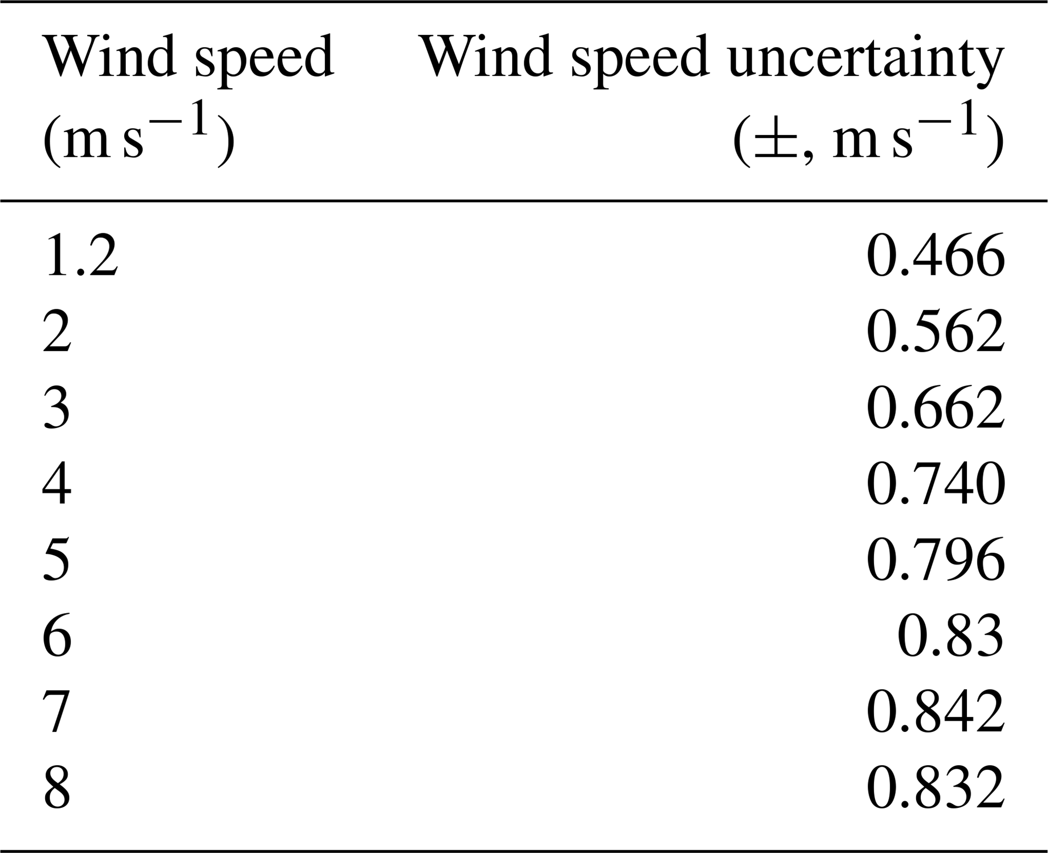
The flux error due to wind field uncertainty mainly comes from wind speed uncertainty. In order to quantify the wind speed uncertainties, the 1-month wind profile data at the height of 250 m during the time period 09:00–16:00 LT (UTC+8) from 1 to 30 April 2019 were derived from the Doppler wind profile radar located in Shijiazhuang (38.17^∘ N, 114.36^∘ E). The average wind fields and standard deviations were calculated for each hour, as shown in Fig. 4. Two-order polynomials were applied in order to derive the function of standard deviation versus average value for both wind speed and wind direction. Some sample values calculated using these polynomials are listed in Table 3. Table 4 lists all the simulation parameters of NO_x and SO₂ that were required.

Figure 4 Polynomial fitting of the wind speed uncertainty.

Table 3 Wind speed uncertainty and wind direction uncertainty after polynomial fitting.

Table 4 Simulation parameters and data range of NO_x and SO₂.

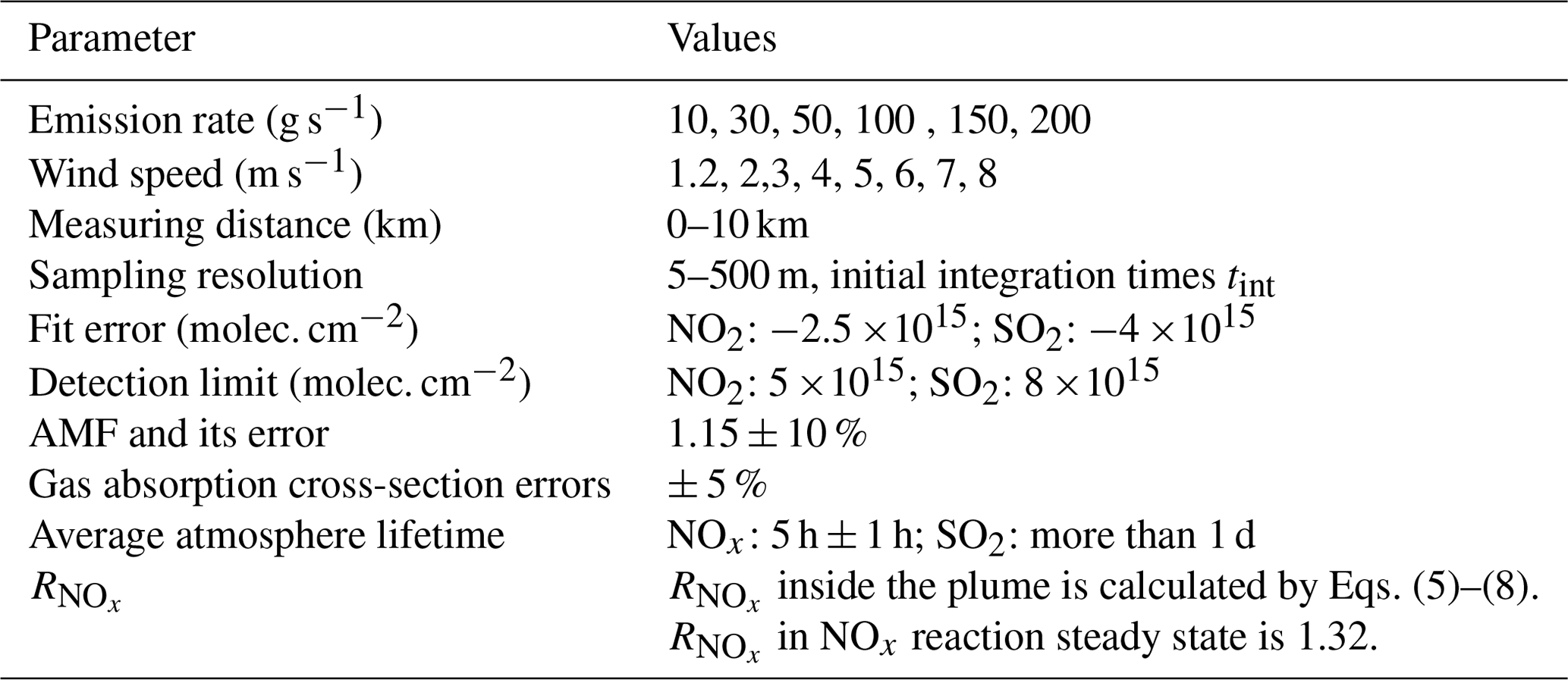
The parameters listed in Table 4 were applied in the forward model in order to perform the simulation. The simulation results are shown in Figs. A1 and B1 of the Appendix.

4 Analysis of emission flux errors measured by mobile DOAS based on the forward model

Figures A1 and B1 in the Appendix show that the modeled relative errors of NO_x and SO₂ emission flux varied with sampling resolution and distance from the point source under different wind speeds and emission rates. Some overall features can be derived from these figures. Therefore, typical cases were selected in order to discuss the overall features based on several key factors.

4.1 Sampling resolution and its error

Sampling resolution variation impacts on the error combination and propagation and its error are an error source.

Sampling resolution is derived from GPS records in actual measurement. The typical uncertainty of the GPS readings is < 1.5 m. For measurements with small sampling resolutions the GPS error can thus cause relatively large uncertainties for the flux contributions from individual measurements (Eq. 1). However, even for small sampling resolutions the GPS errors of neighboring flux contributions almost completely cancel each other out. Thus, the contribution of the GPS error to the flux calculation (Eqs. 16 and 17) can be neglected.

In actual measurements, if one distance is too long, and this happens to be inside the plume, while the next distance is too short but is already outside the plume, the flux will be overestimated in spite of the fact that the sum of the two distances has only a small error. In this case, the sampling error becomes important. The sampling error is largest when the sampling resolution is large. Thus a small and uniform sampling resolution is particularly important.

In order to discuss the dependence of flux error on sampling resolution, some data were extracted from the Appendix and plotted in Fig. 5. This figure shows the increase in relative error with increasing sampling resolution. It should be noted that the smaller the sampling resolution, the more data the mobile DOAS will sample. This directly leads to the inclusion of more data in the emission flux calculations, resulting in the lower emission flux error. However, when far from the source, the plume width narrows quickly (see Sect. 4.2). Applying different sampling resolutions is no longer feasible. Therefore, the sampling resolution can only work effectively when the measurements are not far from the source.

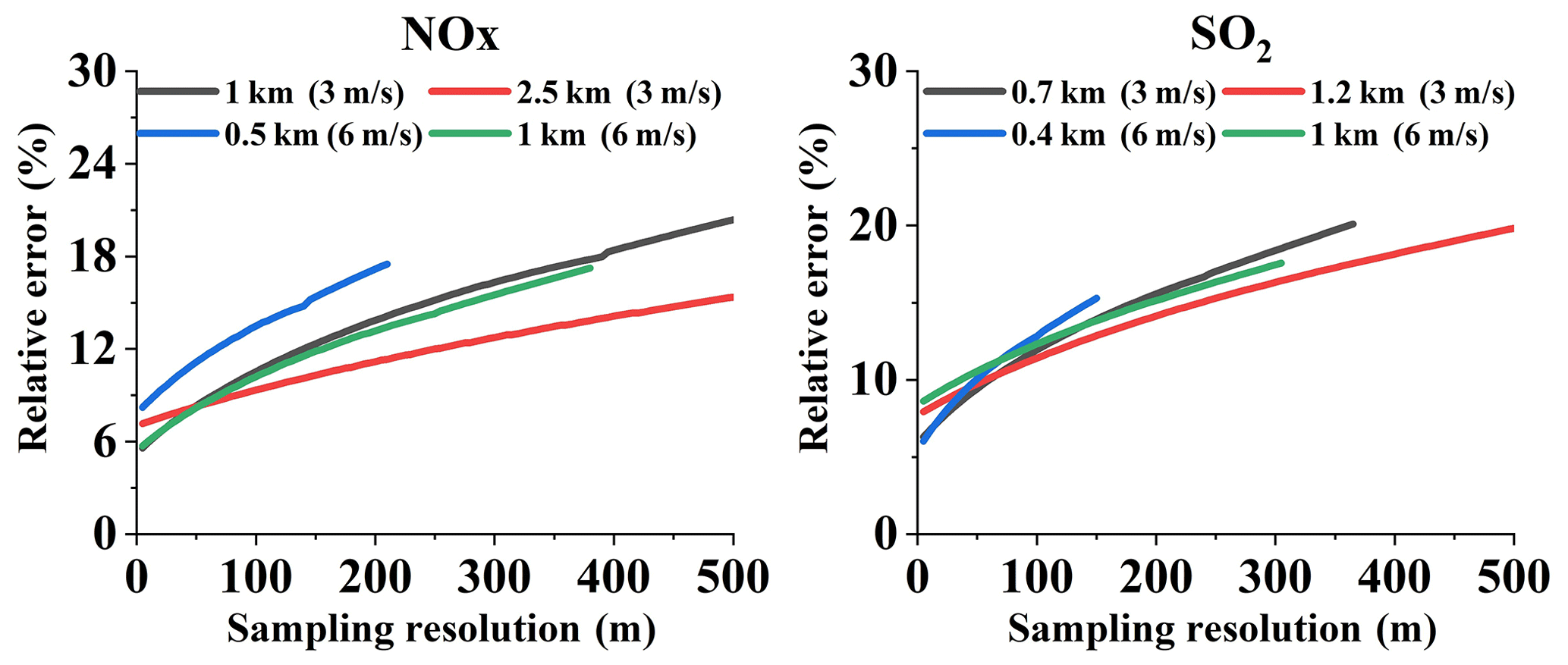
Figure 5 Dependence of relative errors on sampling resolution (Q = 100 g s⁻¹, u = 3, and 6 m s⁻¹, at different measuring distances).

The impact of sampling resolution on emission flux error is noticeable. In terms of measurement efficiency, the sampling resolution should not be too small. Also, to avoid large errors and sampling errors, large resolution is not recommended. Therefore, we recommend the proper sampling resolution be between 5 and 50 m. Larger resolutions may also be viable, but > 100 m is not recommended.

4.2 Measuring distance from the source

Measuring distance is not an error source, but it affects the dispersion and NO_x chemical reactions, further adding to the emission flux error. Figure 6 presents typical examples of relative errors varying with distance at a resolution of 20 m. Wind speeds of 3 and 6 m s⁻¹ were utilized in this example. The overall feature shown in all of the panels of Fig. 6 is the rapid decrease and then quick increase in the relative error with measuring distance. Different factors lead to the large errors at small and large distances.

Figure 6 Variation in NO_x and SO₂ flux relative errors with distance, using Eqs. (16) and (17) (Q = 100 g s⁻¹, setting the sampling resolution s = 20 m and the wind speed to 3 and 6 m s⁻¹).

First, we analyzed NO_x and SO₂ emission flux errors for a large measuring distance. The large distance results in the dramatic decrease in SCDs due to dispersion and decay along the plume transport path. The SCDs can be lower than the detection limit of mobile DOAS measurements, resulting in a portion of the undetectable flux. Because of dispersion, the plume widths with SCDs above the detection limit and thus the detectable fluxes decrease significantly with distance, even dropping to zero, as shown in Fig. 6. This causes the relative error to increase at large measuring distances.

Second, we analyzed NO_x and SO₂ emission flux errors in the case of a small measuring distance. Figure 6 indicates that the error is large and decreases rapidly with increasing measuring distance when close to the source. As discussed in Sect. 4.1, if more measurement data are included in the calculations of flux, the relative error can decrease. When the measuring distance is small, the number of samples can dramatically decrease. For SO₂, the relative error can increase significantly when the measurements are close to the point source. For NO_x, the relative error is also affected by chemical reactions; we will discuss this phenomenon in Sect. 4.4.

4.3 Wind fields and their uncertainties

Wind fields can impact both the gas dispersion (Eqs. 2, 9, and 10) and the calculation of emission flux (Eqs. 1 and 15). In terms of dispersion, wind speed affects gas VCD (Eqs. 9 and 10). In terms of flux calculation, the temporal and spatial uncertainty of wind fields can contribute to emission flux calculation errors. Therefore, the effects of wind fields are discussed based on these two factors in this section.

Figure 7 displays the variations in the relative errors of NO_x and SO₂ with wind speed at different distances. The emission rate Q and the sampling resolution are chosen as 100 g s⁻¹ and 20 m, respectively. Figure 7 indicates the different features of relative error for wind speeds at small and large measurement distances. The relative error of NO_x increases with increasing wind speed at different distances, while the SO₂ relative error for measurements at small distances exhibits a trend opposite that of the large distance measurements. The causes of the different relationships at small and large measurement distances are discussed in Sect. 4.3.1.

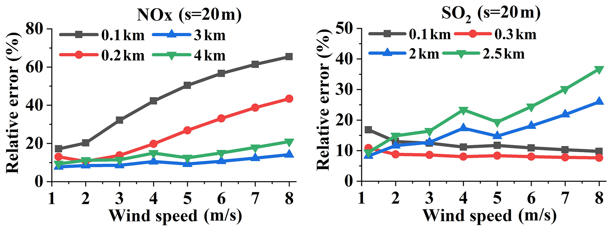
Figure 7 Relative errors of NO_x and SO₂ emission flux changes with wind speed at different measurement distances (Q = 100 g s⁻¹, sampling resolution s = 20 m).

4.3.1 Effects of different wind speeds on measurements at small and large measurement distances

Since the NO_x and SO₂ flux measurement errors of different wind speeds are very different at small and large measurement distances, we discuss them separately.

SO₂

We first analyzed the effect of different wind speeds on the SO₂ emission flux error.

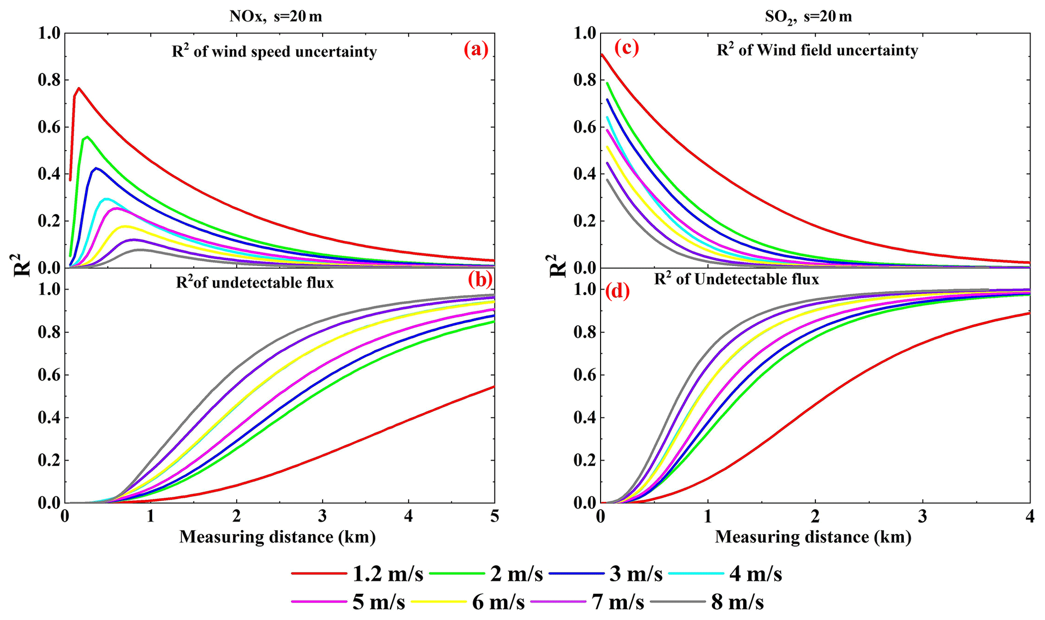
Figure 8 Wind speed uncertainty ratio squared $R_{\mathrm{u}}^{\mathrm{2}}$ (a, c) and undetectable emission flux ratio squared $R_{\mathrm{uf}}^{\mathrm{2}}$ (b, d) of NO₂ and SO₂ emission flux measurement error changes with measurement distance for different wind speeds (Q = 100 g s⁻¹, sampling resolution s = 20 m).

Since VCDs decrease with increasing wind speed (Eqs. 9, 10, and 11), more SCDs would be below the detection limit of mobile DOAS at high wind speeds. Hence, the contribution of undetectable SCDs to the error of flux calculations depends on wind speed. In addition, since wind fields are input into the calculations of emission flux (Eqs. 1 and 15), their uncertainties can contribute to the flux measurement error. In order to investigate the contributions of undetectable ambient VCDs and the influence of wind field uncertainties in flux measurement, the ratios $R_{\mathrm{uf}}^{\mathrm{2}}$ (R² of the undetectable flux) and $R_{\mathrm{u}}^{\mathrm{2}}$ (R² of the wind speed uncertainty) calculated using Eq. (18) are shown in Fig. 8c and d for different wind speeds and measurement distances.

Again, we first analyzed the measurements at large distances. The undetectable VCDs dominate the effect of wind fields on the error of flux calculations when the measurement distance is large. As shown in Fig. 8d, undetectable flux dominates the flux errors when measuring at a large distance. The $R_{\mathrm{uf}}^{\mathrm{2}}$ becomes greater with larger wind speeds, for large measurement distances, as shown in Fig. 8c and d. Therefore, undetectable VCDs dominate the effect of wind fields on the error of flux calculations when the measurement distance is large. Since VCDs decrease with increasing wind speeds, the flux error associated with undetectable VCDs should be increased with wind speed. This relationship explains the phenomenon that the relative error of emission flux increases with increasing wind speed for large measurement distances.

Next, the measurements at small distances were analyzed. Figure 8c and d indicate that $R_{\mathrm{uf}}^{\mathrm{2}}$ is much lower than $R_{\mathrm{u}}^{\mathrm{2}}$ for short measurement distances. The wind field uncertainty dominates the effect of wind fields on the flux calculation errors. Meanwhile, since the relative uncertainty of the wind field decreases with increasing wind speed, the emission flux error decreases with increasing wind speed for short measurement distances, as shown in Fig. 6.

NO_x

We next analyzed the effect of different wind speeds on NO_x emission flux error, as shown in Fig. 9a and b.

Figure 9 Changes of $R_{\mathrm{u}}^{\mathrm{2}}$ and $R_{\mathrm{uf}}^{\mathrm{2}}$ of NO_x and SO₂ emission flux measurement errors with measurement distance for different wind speeds (Q = 100 g s⁻¹).

The effects of different wind speed dispersions on NO_x emission flux error are similar to SO₂, i.e., Fig. 8b and d, indicating that the effects of wind speed dispersion are analogous. The effect of wind field uncertainty is much different from SO₂, however, especially when the measurements are very close to the source. When very close, wind field uncertainty influence increases and then decreases with distance. Compared with SO₂, the decreasing trend of NO_x in the case of far measurement distances is also similar, but the increasing trend is very different. This implies that NO_x measurements close to the source have another main potential error source, which we will investigate in Sect. 4.4.

The four panels in Fig. 8 share the common characteristic that the R² lines have intersections between 4 and 5 m s⁻¹. This implies that the wind field uncertainty effect and the wind field dispersion effect are distinguished between 4 and 5 m s⁻¹. In actual measurements, undetectable VCDs cannot be well quantified. Therefore, we recommend the proper wind speed for mobile DOAS be < 4 m s⁻¹. The appropriate lower wind speed in this study was 1.2 m s⁻¹, but the Gaussian plume model we used becomes increasingly inaccurate when wind speeds are under 1 m s⁻¹. Thus, we recommend a proper wind speed of 1–4 m s⁻¹.

4.3.2 Error budget of undetectable flux and uncertainties of wind speed

The remaining question is what flux error budget is associated with the wind speed. From Sect. 2.6 we know that wind field uncertainties mainly come from the wind speed uncertainties. Undetectable flux is the result of SCDs below the detection limit, but the main driver of the $R_{\mathrm{uf}}^{\mathrm{2}}$ increasing trend along the wind direction is the wind dispersion. Figure 9 presents the changes in $R_{\mathrm{u}}^{\mathrm{2}}$ and $R_{\mathrm{uf}}^{\mathrm{2}}$ of NO_x and SO₂ with distance for different wind speeds, 3 and 6 m s⁻¹.

As for SO₂, the wind field influence contributes most of the emission flux error from wind field uncertainty, in conjunction with wind dispersion. Furthermore, contributions from wind speed uncertainty in the emission flux error are also presented in Fig. 9. This demonstrates that wind speed uncertainty dominates the flux error when measuring close to the source.

With regard to NO_x, the wind speed influence is similar to SO₂ when measuring far from the source and very different when measuring close to the source. As discussed above, mobile DOAS can only measure the NO₂, as opposed to the NO_x. The amount of NO₂ yield determines the mobile DOAS measurement result, and thus that of the NO_x flux measurement error, especially when measuring very close to the source.

4.4 NO_x chemical reactions

In Sect. 4.2, we left the question as to why the NO_x flux error is very large when very close to the source unanswered (see Fig. 6). In this section, we will investigate the reason for this phenomenon.

Stacks mainly exhaust NO, which then transforms into NO₂ in a few minutes due to chemical reactions. Since NO_x disperses along the wind direction, this means that the [NO_x] ∕ [NO₂] ratio varies with distance. With O₃ mixing to the air parcels of the plume continually, more NO₂ would be yielded and [NO_x] ∕ [NO₂] ratio decreases with the distance before the NO_x reaction steady state. For readability, we here show the increasing trend of [NO₂] ∕ [NO_x] ratio along the distance in Fig. 10a.

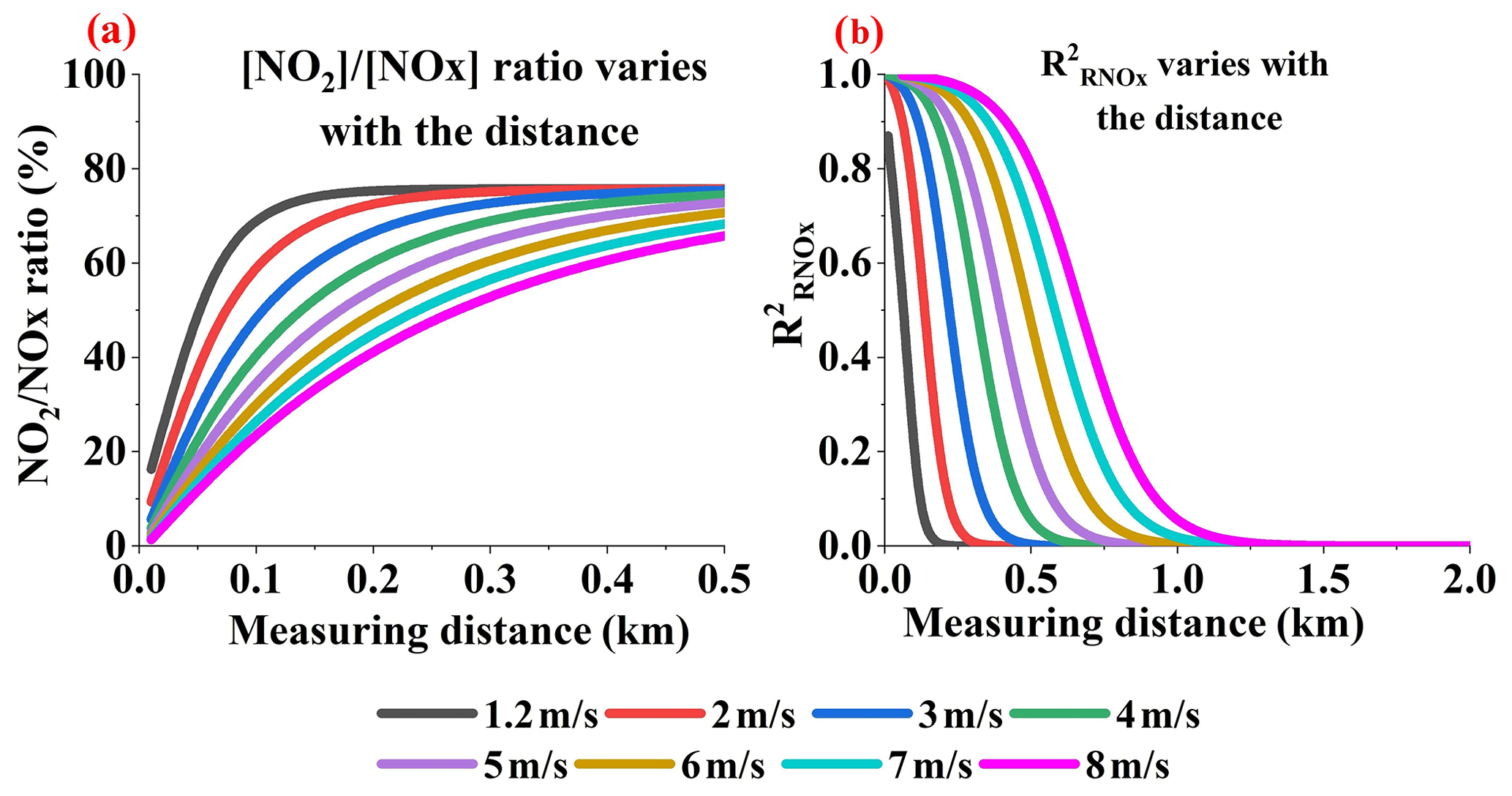
Figure 10 Variation in [NO₂] ∕ [NO_x] ratio (a) $R_{R_{{\mathrm{NO}}_x}}^{\mathrm{2}}$ with distance (b) at different wind speeds (Q = 100 g s⁻¹).

In actual measurements, especially for elevated point sources, the dependence of the [NO_x] ∕ [NO₂] ratio on the distance from the air parcels of the plume is difficult to measure. The [NO_x] ∕ [NO₂] ratio could, for example, be measured by an in situ instrument on the ground. However, in some cases the plume might not reach the ground. And even if it reaches the ground the measured [NO_x] ∕ [NO₂] ratio is probably not representative for the whole plume. Furthermore, the ambient [O₃] could also be measured, which would help to constrain the [NO_x] ∕ [NO₂] ratio. Also, if O₃ measurements are available, the calculation of the [NO_x] ∕ [NO₂] ratio will have its uncertainties, and the derived [NO_x] ∕ [NO₂] ratio will again not be representative for the whole plume. Thus in our study, we calculate the [NO_x] ∕ [NO₂] ratio based on the dispersion model with some additional assumptions which are outlined in the text. In this way we can derive the general dependencies of the [NO_x] ∕ [NO₂] ratio on the plume distance and apply a corresponding correction. However, for the NO_x flux calculations, even after the application of the [NO_x] ∕ [NO₂] ratio correction factor, substantial flux errors near the source might occur.

Figure 10b displays the $R_{R_{{\mathrm{NO}}_x}}^{\mathrm{2}}$ value of the [NO_x] ∕ [NO₂] ratio correction error. The larger the [NO_x] ∕ [NO₂] ratio, the larger the $R_{R_{{\mathrm{NO}}_x}}^{\mathrm{2}}$ value of the [NO_x] ∕ [NO₂] ratio correction. This causes the $R_{R_{{\mathrm{NO}}_x}}^{\mathrm{2}}$ to increase, to as high as 1, when near the source. Also, from the $R_{R_{{\mathrm{NO}}_x}}^{\mathrm{2}}$ value we discovered that the [NO_x] ∕ [NO₂] ratio correction error is the main error source when close to the emission source. Hence, the main flux error source near the emission source is the [NO_x] ∕ [NO₂] ratio correction error.

Since we know that the [NO_x] ∕ [NO₂] ratio correction error is the main error source near the emission source, developing ways to avoid or minimize this error is our goal.

Figure 11 Variation in $r_{{\mathrm{NO}}_{\mathrm{2}}}/r_{max}$ with time (a), NO_x steady-state distance from the source (b), and $E_{R_{{\mathrm{NO}}_x}}$ values (c) under different emission rates and wind speeds ([O₃] = 1.389 ×10¹² molec. cm⁻³).

In real-world experiments, accurately measuring NO_x flux requires NO_x to reach a steady state. According to Eq. (3), when time approaches infinity, the NO₂ reaction rate $r_{{\mathrm{NO}}_{\mathrm{2}}}$ approaches 0, indicating that NO_x reaches a steady state. In theory, steady-state NO_x is an ideal condition for measuring NO_x flux. Infinite time, however, is not our expectation. If we regard $r_{{\mathrm{NO}}_{\mathrm{2}}}=\mathrm{0.05}{r}_{max}$ as the approached steady state, the approached steady-state time could be attained, as well as the approached steady-state distance. r_max is defined as the theoretical NO₂ maximal reaction rate, which is $r_{{\mathrm{NO}}_{\mathrm{2}}}=k_{\mathrm{5}}\left[\mathrm{NO}{]}_{\mathrm{0}}\right[{\mathrm{O}}_{\mathrm{3}}]$. Figure 11a displays the variation in $\frac{r_{{\mathrm{NO}}_{\mathrm{2}}}}{r_{max}}$ with time, and Fig. 11b displays the approached steady-state distance.

In order to investigate the feasibility of our recommendation, we used the following equation for analysis:

$$\begin{array}{}\text{(19)}& E_{R_{{\mathrm{NO}}_x}}={\displaystyle \frac{\mathrm{\Delta }{F}_{R_{{\mathrm{NO}}_x}}}{DQ}}\times \mathrm{100}\mathit{\%},\end{array}$$

where $\mathrm{\Delta }{F}_{R_{{\mathrm{NO}}_x}}$ is the flux error resulting from the [NO_x] ∕ [NO₂] ratio correction at the approached steady-state distance. $E_{R_{{\mathrm{NO}}_x}}$ is used rather than R² because R² only represents the error source contribution and budget. For example, the R² value of the [NO_x] ∕ [NO₂] ratio correction error is 0.9, while the total relative error is only 10 %. In this case, it seems that we cannot accept the high R², although the total relative error is acceptable. Therefore, in our judgment, using $E_{R_{{\mathrm{NO}}_x}}$ is an advantage.

The $E_{R_{{\mathrm{NO}}_x}}$ values at the approached steady-state distance for different wind speeds and emission rates were calculated, and the results are presented in Fig. 11c. From this figure, we can infer that $E_{R_{{\mathrm{NO}}_x}}$ is approximately 5 %, which is very low. This indicates that the flux error resulting from the [NO_x] ∕ [NO₂] ratio correction at the approached steady-state distance is very small and can thus be regarded as negligible.

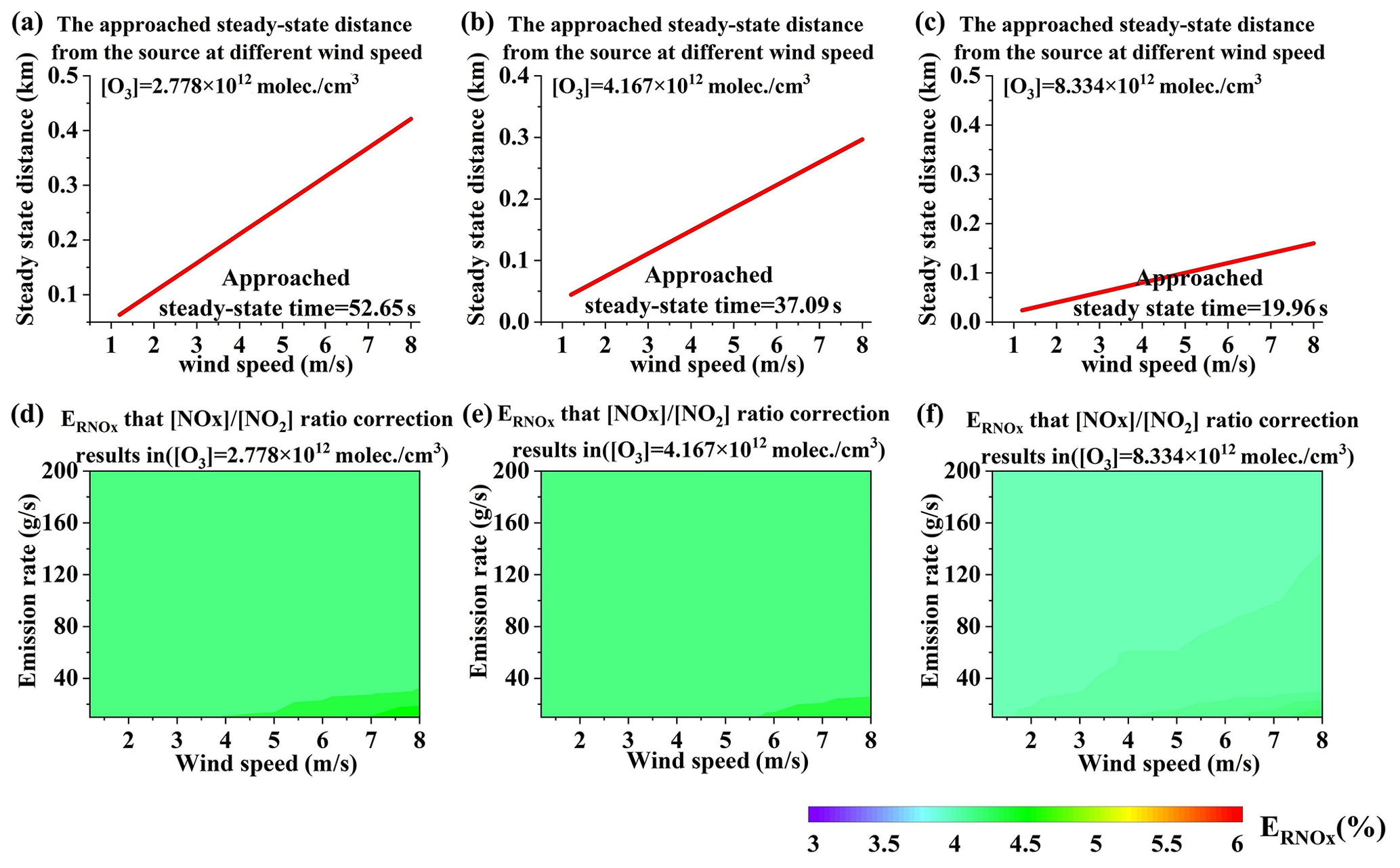
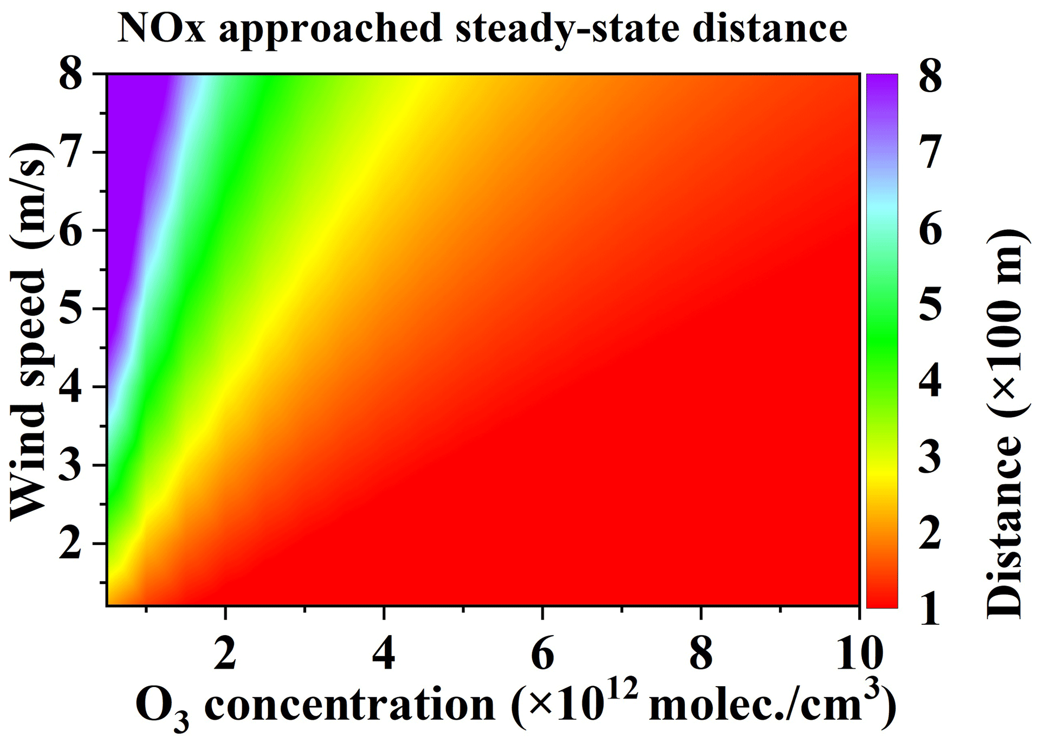
Figure 12 NO_x approached steady-state distance from the source (a–c) and $E_{R_{{\mathrm{NO}}_x}}$ values (d–f) under different emission rates, different wind speeds, and different [O₃] values.

According to Eq. (3), $r_{{\mathrm{NO}}_{\mathrm{2}}}$ depends on [O₃]. Hence, we also calculated the NO_x steady-state distance and $E_{R_{{\mathrm{NO}}_x}}$ under different [O₃] values. The $E_{R_{{\mathrm{NO}}_x}}$ was also approximately 5 % under different [O₃] values, as shown in Fig. 12. The dependence calculation demonstrates that $E_{R_{{\mathrm{NO}}_x}}$ is also very small under different [O₃] values. Consequently, regarding $r_{{\mathrm{NO}}_{\mathrm{2}}}=\mathrm{0.05}{r}_{max}$ as the approached steady state seems to be acceptable.

In summary, when very close to the emission source, the main flux error source is the [NO_x] ∕ [NO₂] ratio correction error. In order to avoid or minimize this error, we recommend $r_{{\mathrm{NO}}_{\mathrm{2}}}=\mathrm{0.05}{r}_{max}$ as the approached steady state, in which case the approached steady-state distance is the starting measurement distance. The overall distances for different [O₃] concentrations were also simulated as a reference for the DOAS measurement of NO_x point source emissions, as shown in Fig. 13.

Figure 13 NO_x steady-state distance from the source for different [O₃] concentrations ($r_{{\mathrm{NO}}_{\mathrm{2}}}=\mathrm{0.05}{r}_{max}$).

4.5 Undetectable flux

As discussed in Sect. 4.3, undetectable flux dominates the flux error when far from the source. In the following, we discuss further details of the undetectable flux error. The undetectable flux is caused by SCDs below the detection limit. Following Platt and Stutz (2008), we set the detection limit as 2 times the fit error. While the exact value of the detection limit might be different for different instruments and measurement conditions, we use this value to derive the general dependencies of this error term and its contribution to the total flux error.

Figure 14 NO_x and SO₂ absolute flux error and the $R_{\mathrm{uf}}^{\mathrm{2}}$ that undetectable SCDs result in (Q = 100 g s⁻¹).

VCDs are sensitive to wind speeds and the dispersion (Eqs. 9 and 10); so is the undetectable flux. We calculate the undetectable flux and its $R_{\mathrm{uf}}^{\mathrm{2}}$ along wind direction (equal to that along the measuring distance) as shown in Fig. 14 (for an emission rate of 100 g s⁻¹). As discussed, the main driver of undetectable flux increasing trend along the wind direction is attributed to the wind dispersion, as can be seen from Fig. 14. With measuring distance far away, the undetectable flux gradually dominates the flux error, which can be denoted by the $R_{\mathrm{uf}}^{\mathrm{2}}$ trend. A large wind speed also results in quick dispersion, thus leading to more undetectable flux. The $R_{\mathrm{uf}}^{\mathrm{2}}$ and the undetectable flux increase rapidly under the wind speed of 8 m s⁻¹ than that of 1.2 m s⁻¹ for both NO_x and SO₂.

4.6 Gas absorption cross-section error

As discussed in Sect. 2.6, the gas absorption cross-section error contribution to SCD errors is independent of the SCD fit error. Uncertainties of the trace gas cross sections cause systematic SCD uncertainty. We calculated $R_{\mathrm{cro}}^{\mathrm{2}}$ along the wind direction and the total relative errors at the speed of 1.2 and 8 m s⁻¹, as shown in Fig. 15. The $R_{\mathrm{cro}}^{\mathrm{2}}$ variation trend is similar to $R_{\mathrm{uf}}^{\mathrm{2}}$ in Sect. 4.6 due to the relative error variation. However, maximum $R_{\mathrm{cro}}^{\mathrm{2}}$ has a subtle difference but varies apparently along the wind direction under different wind speed, which indicates that $R_{\mathrm{cro}}^{\mathrm{2}}$ is not very sensitive to wind speeds but sensitive to the dispersion. From Fig. 15 we see that $R_{\mathrm{cro}}^{\mathrm{2}}$ could approach 0.5, which means that gas cross-section error might even become the main error source. However, when $R_{\mathrm{cro}}^{\mathrm{2}}$ is close to 0.5, the relative errors of NO_x and SO₂ are at low levels. This further suggests the trace gas cross-section error has an overall small contribution to the total flux error.

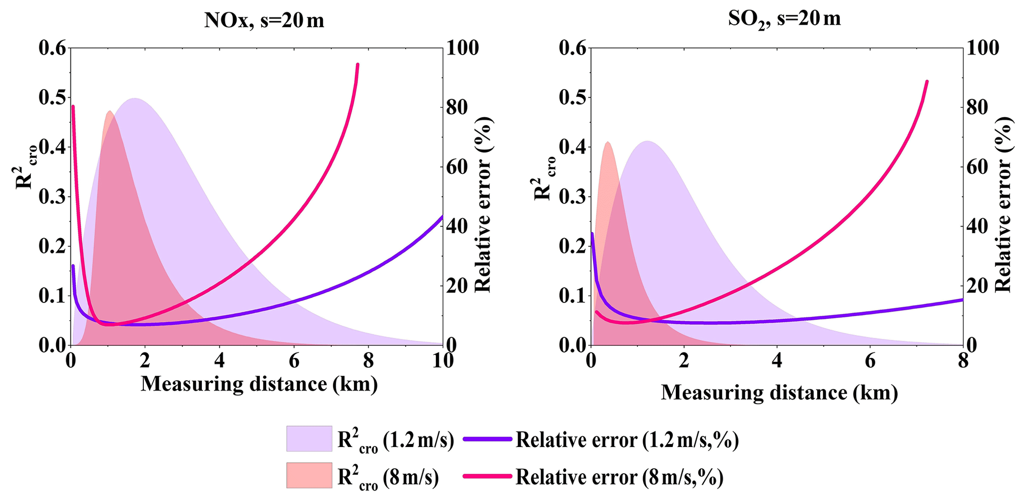
Figure 15 NO_x and SO₂ $R_{\mathrm{cro}}^{\mathrm{2}}$ of absorption cross-section error under different wind speeds (Q = 100 g s⁻¹).

4.7 AMF error

AMF values depends on plume height, SZA and aerosol optical density (AOD) as shown in Fig. 16. For plume heights < 50 m, the AMF is around 1.03 and its error can be neglected. For plume heights 250 m, the AMF error is about ± 10 %. Since the plume height in our study is about 250 m, the contribution from the AMF error has to be taken into account.

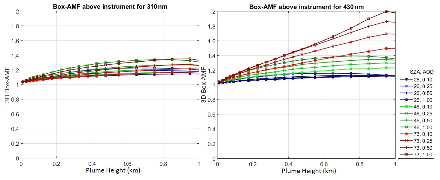
Figure 16 The 3D box AMF dependence on plume height, SZA, and aerosol optical density (AOD) for 310 and 430 nm. For the aerosols a box profile between the surface and 1 km was assumed.

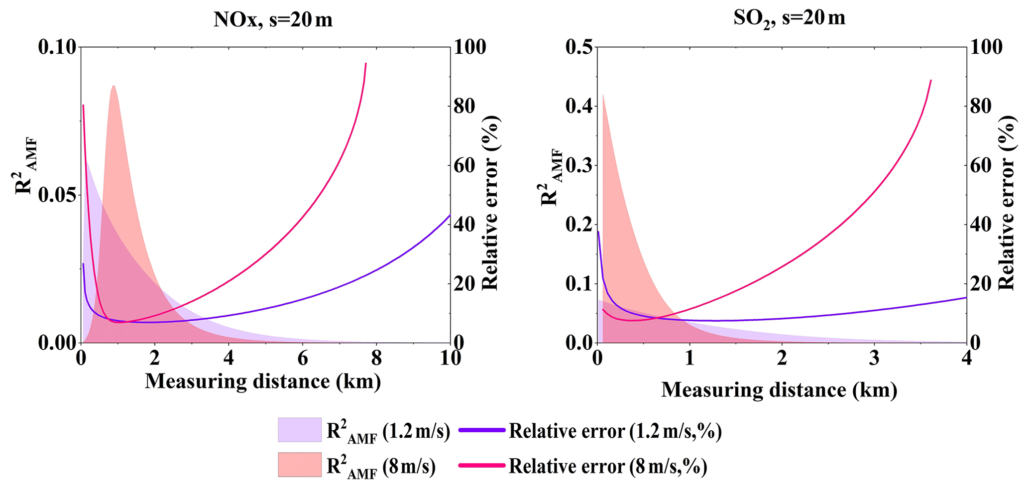
Figure 17 NO_x and SO₂ total relative error and $R_{\mathrm{AMF}}^{\mathrm{2}}$ of AMF error under different wind speed (Q = 100 g s⁻¹, s = 20 m).

Since VCDs are derived from SCDs by dividing the AMF, then AMF errors introduce VCD errors, which furthermore contribute to the emission flux errors. Wind speed uncertainty is the main error source when close to the source. With larger wind speed, the relative error of the wind speed becomes smaller, which then also contributes less to the flux error. This indicates that the flux error that results from other error sources, such as the AMF error, have larger relative contributions under larger wind speed. Figure 17 presents $R_{\mathrm{AMF}}^{\mathrm{2}}$ and the total relative errors for wind speeds of 1.2 and 8 m s⁻¹. From Fig. 17 we could see that $R_{\mathrm{AMF}}^{\mathrm{2}}$ for SO₂ under the speed of 1.2 m s⁻¹ is very small while it becomes larger at the speed of 8 m s⁻¹, even near 0.5 when near the source. The NO_x flux error, however, is less affected by the AMF error for $R_{\mathrm{AMF}}^{\mathrm{2}}$ < 0.1.

4.8 Effect of number of measurement times

In our experiments, we only simulated a single scan of the plume by the mobile DOAS at each specific distance. In reality, we usually scan the plume cross section several times in order to reduce the flux error. The elapsed time between two scans at the same distance from the source is then also an important parameter. The more elapsed time, the greater the uncertainties due to temporal variations in the flux and/or the wind fields. Here, we assumed that the elapsed time is small and its influence can thus be neglected in our simulation. Figure 18 displays the simulation example of NO_x and SO₂ flux error under different measurement times.

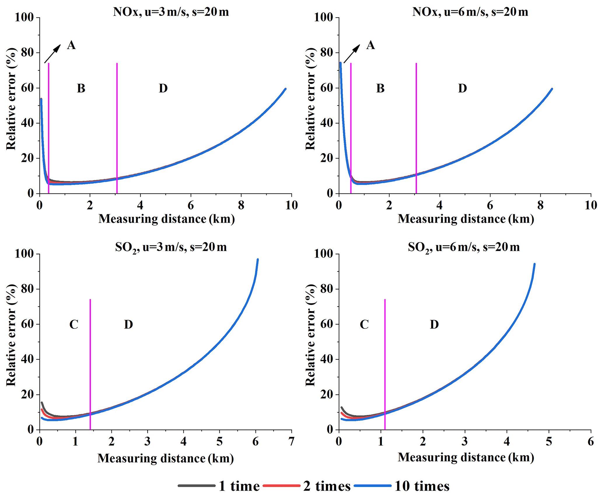
Figure 18 Emission flux error under different numbers of scans. Range A is very close to the source, range B is not too close or too far, range C is close to the source, and D is far from the source (Q = 100 g s⁻¹).

The error sources of the emission flux can be classified into two types. The first is the measurable error and uncertainty: wind speed uncertainty, AMF error, and undetectable flux. The second is [NO_x] ∕ [NO₂] ratio correction error near the source and the gas absorption cross-section error. The flux error resulting from the first type of error source can be lowered by scanning the plume more times while the second cannot. Undetectable SCDs result in undetectable flux, and it can be reduced by more measurement times in theory. In reality, this is often not possible because it requires that all measurement conditions (e.g., the wind field or the background concentrations) stay unchanged. This means that it is hard to lower the undetectable flux by more time scanning in the actual measurements, although it can be easily realized in theory. Therefore, in practice the undetectable flux error also belongs to the second type of errors, which cannot be reduced by multiple measurements.

According to the analysis in Sect. 4.3, the undetectable flux is the main error source when far from the emission source. Consequently, the flux error under different numbers of scans for both NO_x and SO₂ cannot be significantly lowered when measuring far from the source (range D in Fig. 18). Within the close measurement range (range C in Fig. 18), the first type of error source is the predominant source of SO₂ error, and thus the flux error can be lowered by additional plume scans. For NO_x, however, the [NO_x] ∕ [NO₂] ratio correction error is the main error source when very close to the emission source (range A in Fig. 18), and thus the effect of additional plume scans is not evident. A little farther from the source, the first type of error source becomes the main error source (range B in Fig. 18). Ultimately, the impact of additional plume scans becomes effective.

4.9 Effect of spectrometer integration times

Spectrometer noise is the main noise source of the mobile DOAS instrument (Platt and Stutz, 2008; Danckaert et al., 2015). The noise level varies under different integration times, thereby changing the fit error and detection limit, which would then affect the flux measurement error. Therefore, this section is focused on the effect of spectrometer integration times on mobile DOAS flux measurement error.

The relationships among fit error, detection limit, and noise level are (Kraus, 2006; Platt and Stutz, 2008)

$$\begin{array}{}\text{(20)}& {\mathrm{SCD}}_{\mathrm{fit}}\propto {\mathrm{Fit}}_{\mathrm{err}}\propto \mathit{\sigma },D_{\lim }\propto \mathit{\sigma },\end{array}$$

where SCD_fit is the SCD fitting error, Fit_err is the residual in DOAS fitting, D_lim is the detection limit, and σ is the noise level. The noise level is approximately inversely proportional to the square root of the integration times.

The sampling resolution of mobile DOAS can be expressed as

$$\begin{array}{}\text{(21)}& s=v\cdot \left(t_{\mathrm{s}}\cdot n\right)=v\cdot t_{\mathrm{int}},\end{array}$$

where v is the car speed, t_s is a single integration time of the spectrometer, n is the spectrometer averaging times, and t_int is the spectrometer integration times.

According to Eq. (21), the effect of integration times can be investigated in two different ways: Varying the car speed and thus fixing the sampling resolution or fixing the car speed and thus varying the sampling resolution. In this study, we simulated the integration times for 0.25t_int, 0.5t_int, 1t_int, 2t_int, and 4t_int.

4.9.1 Prescribed sampling resolution

Since different integration times result in the car speed varying in a large range in which car speed cannot be fully realized in actuality at a given sampling resolution, the sampling resolution cannot be too small. Here, we chose a 50 m sampling resolution as a case study.

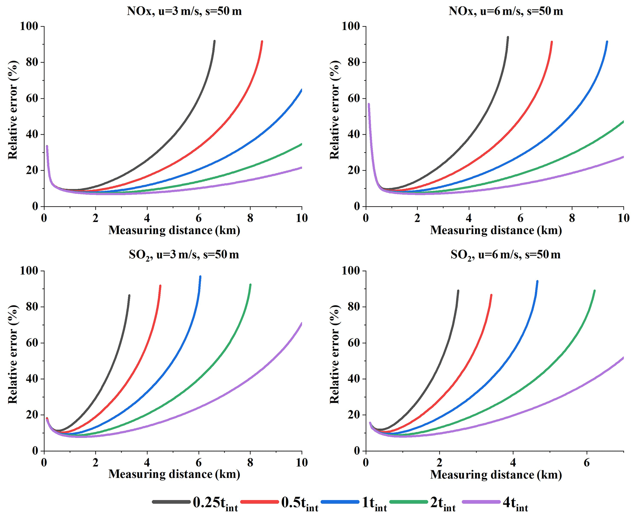
Figure 19 Relative error under different integration times at a prescribed sampling resolution (Q = 100 g s⁻¹).

Figure 19 displays the relative error under different integration times at a given sampling resolution (Q = 100 g s⁻¹). From Fig. 19 we can see the relative error differences resulting from various integration times.

Since a larger integration time will directly lead to a lower detection limit and a smaller fitting error, and indirectly to a lower undetectable flux and a lower fit error, the relative error nonlinearly decreases with increasing integration times. Since the relative error differences caused by integration times become more evident when far from the source (range B in Fig. 19), our analysis focused on this range. This phenomenon is due to that fact that different integration times mainly act on the fit error and the detection limit. Therefore, we separately analyzed these two error sources.

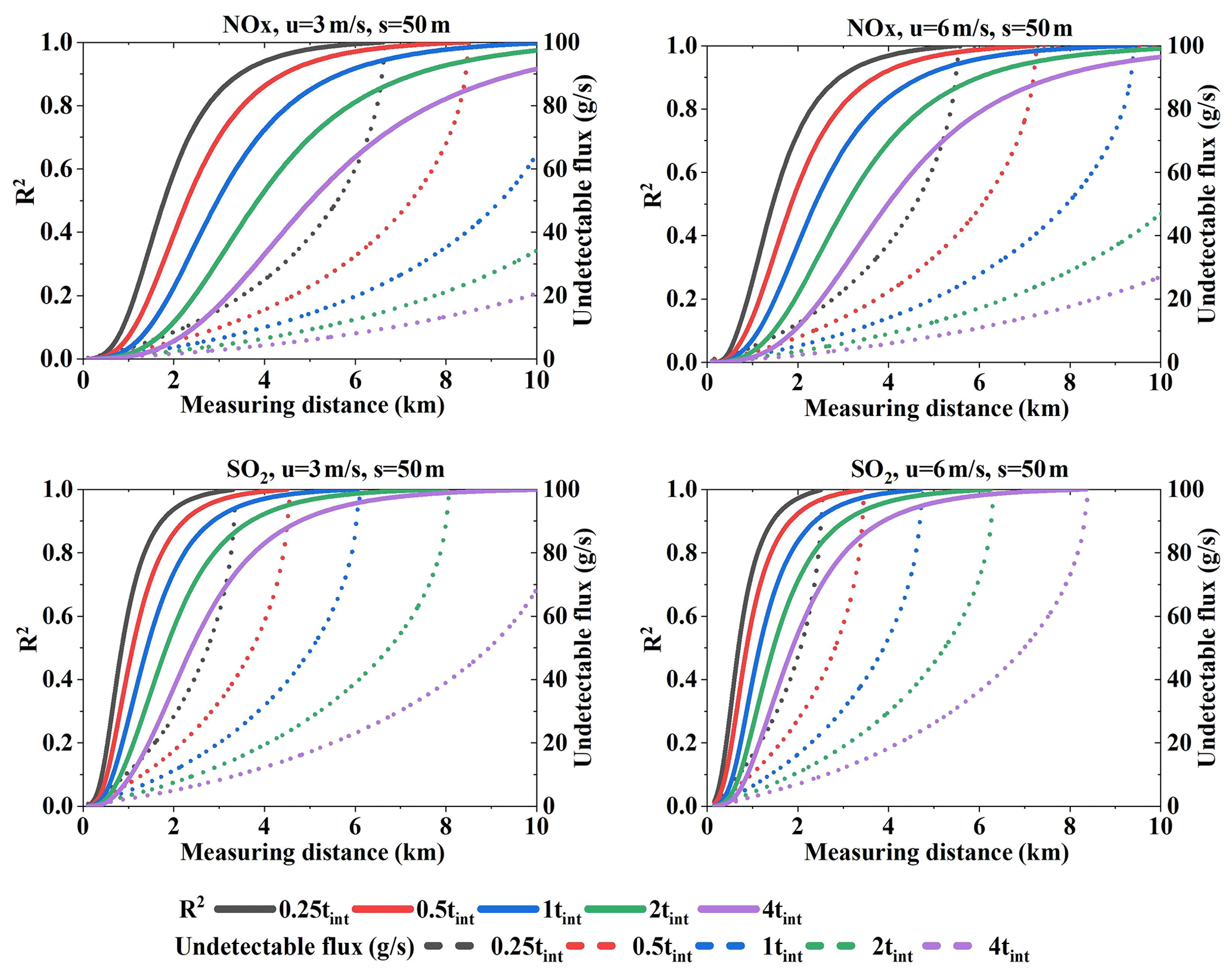
Figure 20 Undetectable flux and its R² values under wind speeds of 3 and 6 m s⁻¹ for NO_x and SO₂ under different integration times. The sampling resolution is 50 m (Q = 100 g s⁻¹).

We analyzed the undetectable flux differences resulting from different detection limits. Figure 20 presents the undetectable flux and its R² values. From the R² values we could infer that undetectable flux contributes most to the error when far from the source. Especially for smaller integration times, undetectable flux R² increases very quickly with distance. In addition, the variation trend of undetectable flux when far from the source corresponds to the relative error trend. Therefore, we infer that the relative error trend under different integration times is determined by the undetectable flux.

In brief, different integration times significantly impact the relative error at a given sampling resolution when far from the source, and these error differences are mainly attributed to the undetectable flux differences resulting from the detection limit.

4.9.2 Prescribed car speed

When the car speed is prescribed, the sampling resolution is determined by the integration times. Therefore, an effect on the error due to the sampling resolution would be introduced (Sect. 4.1).

Figure 21 presents the relative error under different integration times at a given car speed. It is interesting that the relative error differences caused by integration times in ranges B and D (NO_x) are opposite those of ranges C and D (SO₂). We have analyzed the causes of the relative error differences in range D, but we did not analyze the causes in range B or C.

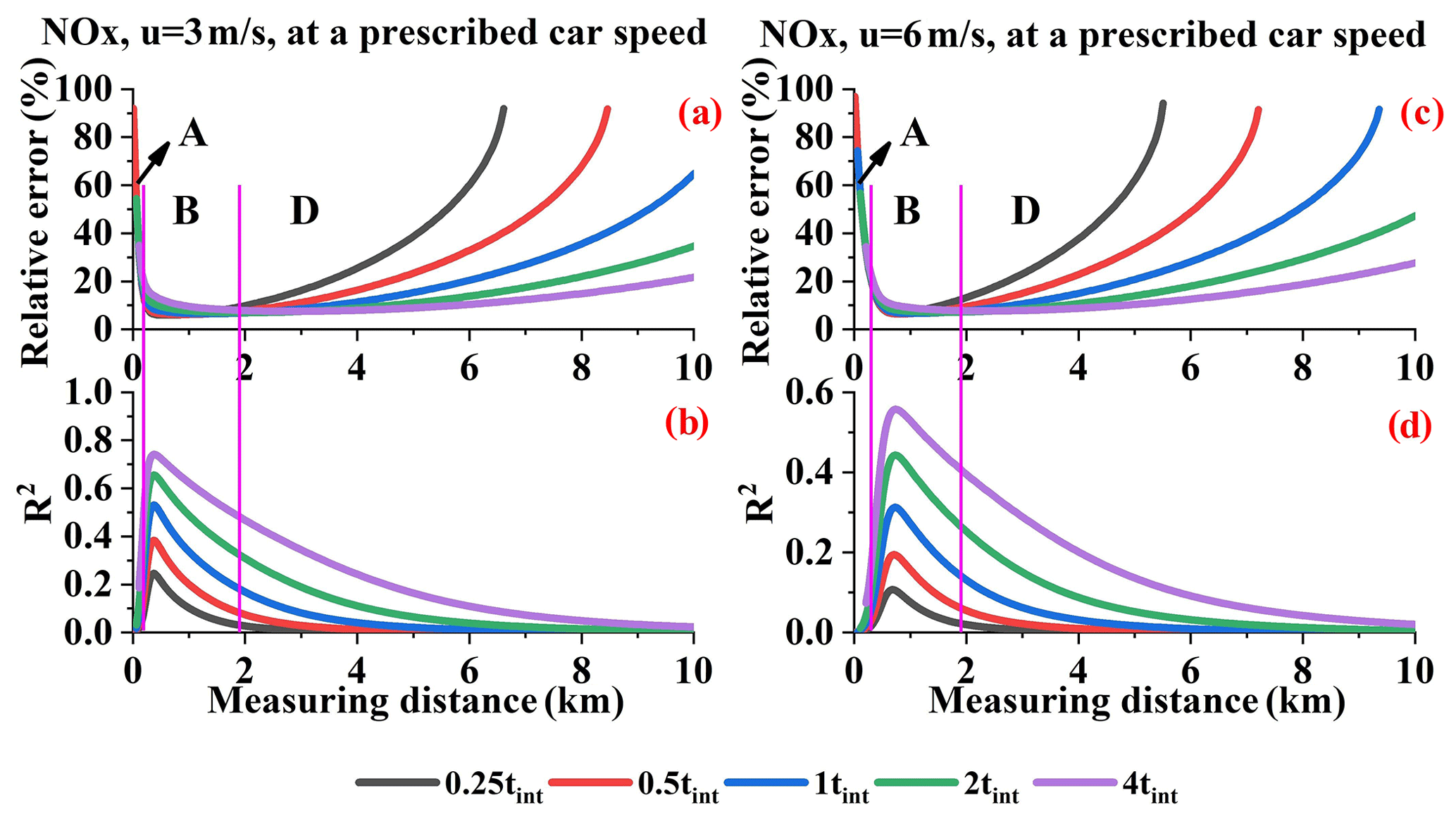
Figure 21 NO_x relative errors (a, c); R² values introduced by the wind field uncertainty AMF error (b, d) (Q = 100 g s⁻¹).

From Sect. 4.1 we know that, within the proper resolution range, the relative error increases with increasing sampling resolution. Moreover, the sampling resolution can only affect the first type of error source mentioned in Sect. 4.6, i.e., the wind speed uncertainty, and AMF error. We calculated the sum of the R² values for the wind field uncertainty and fit error. In addition, the sum of the absolute flux errors introduced by these error sources is shown in Fig. 22. The R² values indicate that, in range B or C, these factors are the main error source and thus cause the differences under different t_int values. The flux error trends do not all correspond to the relative error trend due to the undetectable flux, although it is still the main error source that determines the differences in range B or C.

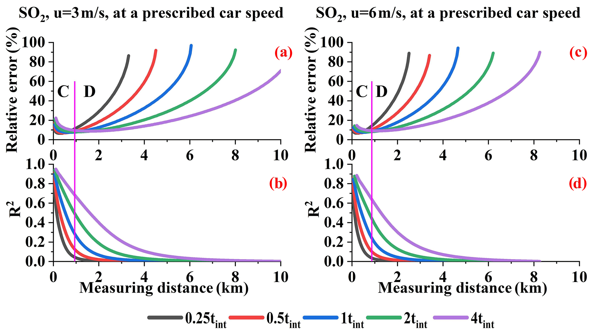
Figure 22 SO₂ relative errors (a, c), R² values, and flux errors introduced by the wind field uncertainty and AMF error (b, d) under wind speeds of 3 and 6 m s⁻¹ (Q = 100 g s⁻¹).

Furthermore, we can conclude that the different integration times that significantly affect the relative error at a given car speed can be divided into two ranges: B and D for NO_x and C and D for SO₂. In ranges B and C, the differences under different t_int values can be attributed to the sampling resolution effect. In range D, the differences under different t_int values can be attributed to the undetectable flux.

Different integration times result in different fit errors and different detection limits. The analysis in terms of either a given sampling resolution or a given car speed has significant implications. For example, when measuring close to the source, i.e., range B or C in Figs. 21 and 22, we can fix the car speed within a proper low integration time in order to obtain a higher resolution, which indirectly results in a lower error. When measuring far from the source, proper large sampling resolutions are available since the main error source is the undetectable flux. This further suggests that larger integration times and higher car speeds can be applied in order to increase the efficiency of measuring flux.

4.10 Effects from other factors

Measuring emission flux is extremely complex. It is feasible to analyze the error caused by some key factors, but it is also necessary to study other factors.

4.10.1 Emission rate

Emission rate is an objective factor. The simulation results suggest that the emission rate significantly affects the relative error distribution. Therefore, disregarding the emission rate in order to analyze the error is a less rigorous approach.

From Eqs. (9)–(11) we know that VCD(x,y) is proportional to the emission rate, which means that lower emission rates generate lower VCD(x,y), leading to a reduction of the measurable plume width with SCDs above the detection limit. Ultimately, this results in larger emission flux errors at the same distance when the emission rate is low, even if there is no proper resolution to measure. In order to achieve a low emission flux error, emission rates that are too low are not recommended. We cannot provide a precise lower limit for the emission rate, but we can propose a range of values. From the figures in the Appendix, we can see that the red areas (indicating large errors) cover nearly all of the figure when the NO_x emission rate is < 30 g s⁻¹ and the SO₂ emission rate is < 50 g s⁻¹. Therefore, emission rates < 30 g s⁻¹ for NO_x and < 50 g s⁻¹ for SO₂ are not recommended in mobile DOAS measurements.

4.10.2 Different source heights

The mobile DOAS height, which is approximately 2 m from the ground to the telescope, is usually negligible in actual measurements. When the source is not very high, however, more gas will descend to the ground under the mobile DOAS telescope, where it cannot be measured. Here, we simulated the emission source at heights of 10, 20, 50, 100, and 200 m. Since lower wind speeds will lead to gas quickly descending to the ground, we simulated a low wind speed of 3 m s⁻¹. The emission rate was set to 100 g s⁻¹.

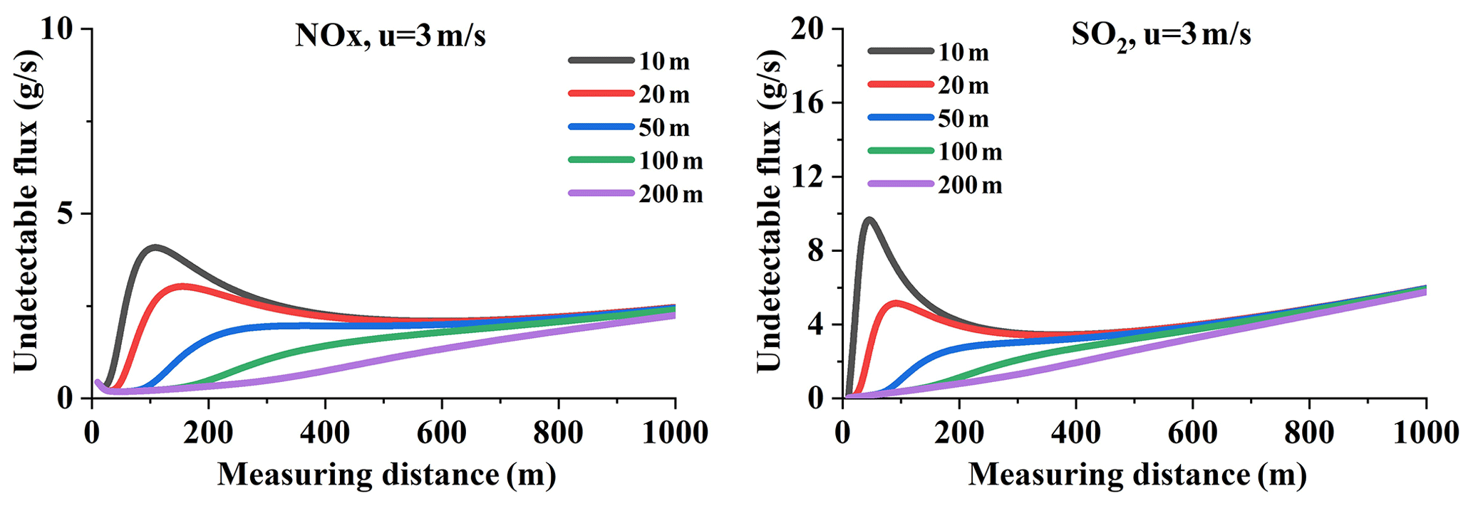
Figure 23 NO_x and SO₂ undetectable flux values at different source heights (Q = 100 g s⁻¹, u = 3 m s⁻¹).

The lower the source height, the more gas will descend to the ground, resulting in changes to the undetectable flux. Figure 23 displays the undetectable flux of NO_x and SO₂ for the wind speed of 3 m s⁻¹. From this figure we can see that obvious variations occur in the NO_x and SO₂ undetectable flux when close to the source. The undetectable flux variation may impact the flux relative error.

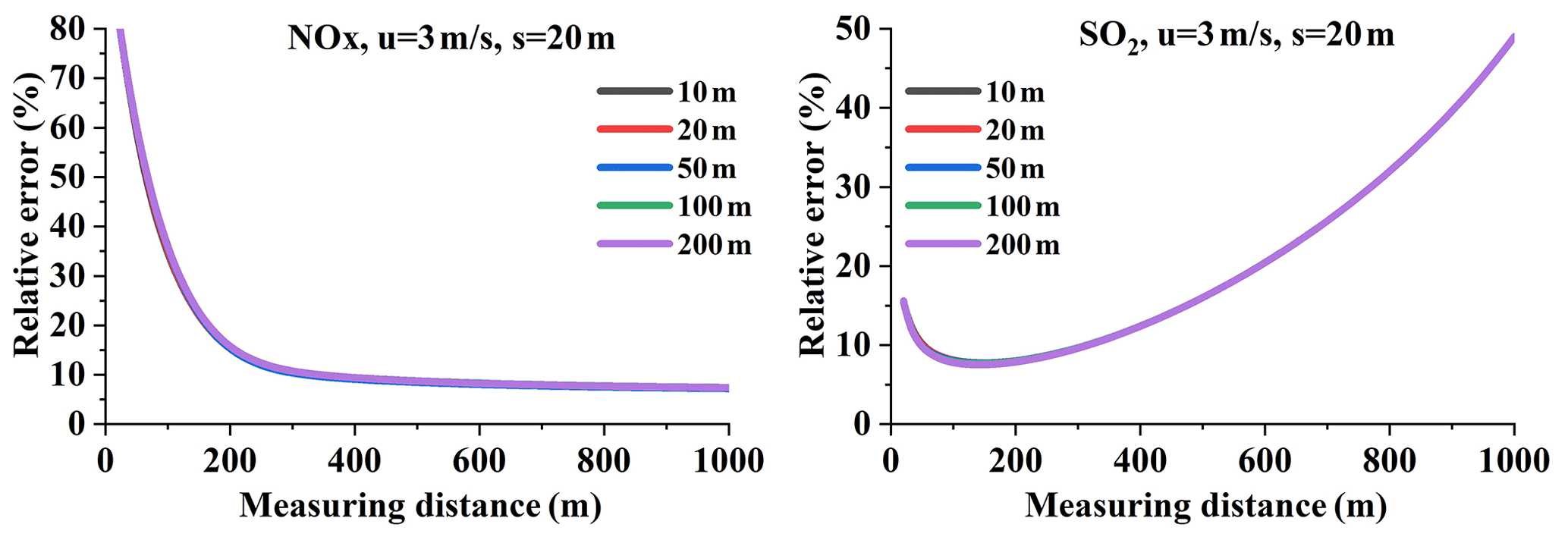
Figure 24 NO_x and SO₂ flux relative errors at different source heights (Q = 100 g s⁻¹, u = 3 m s⁻¹, s = 20 m).

Figure 24 presents the flux relative error at different heights. These results show that the relative errors of NO_x and SO₂ exhibit little variation. This is because, compared to the flux error resulting from other main error sources, the undetectable flux variation with height is negligible.

4.10.3 Uncertainties of the Gaussian dispersion model

The Gaussian dispersion model was assumed in the forward model during our discussion of the emission flux error budget. The dispersion in actual measurements, however, depends on meteorological conditions and surrounding terrain. Also a non-Gaussian behavior of the plume and vertical wind shear might contribute to the total flux error. Thus, the results of this study should be seen as a lower limit of the total flux errors. In some cases, for NO₂, the stratospheric absorption might also become important. However, this might only happen for very long measurement durations or for measurements at high SZA. Differences in the Gaussian dispersion model from reality could have resulted in a bias of the error budget presented in this study from reality. Investigation of the details of the dispersion model is outside the scope of this investigation.

5 Conclusions

In this study, we used a Gaussian dispersion model to quantify the NO_x and SO₂ point source emission flux errors of mobile DOAS.

We first established a forward model for the simulation.

In the forward model, we modified the Gaussian dispersion model in order to make it appropriate for the DOAS technique, i.e., the SO₂ and NO_x VCD dispersion model. The NO_x VCD dispersion model also took NO_x atmospheric chemical reactions into consideration.

Second, we analyzed the simulation data, reaching the following conclusions.

1. The impact of sampling resolution on emission flux error is noticeable. Smaller resolution can lower the flux error. In terms of measurement efficiency, the sampling resolution should be moderate. Therefore, we recommended the proper sampling resolution to range from 5 to 50 m. Larger resolutions could also be applied, but > 100 m is not recommended.

2. Measuring distance significantly affects the flux measurement error. When far from the source, undetectable flux from the wind dispersion effect, which results in large errors, will be noticeable. When close to the emission source, a low number of sampling data leads to large flux errors. The proper measuring distance is not too far or too close to the source. Due to the complex situation, the proper distance is difficult to quantify. It should be noted that undetectable flux is the error source which was not considered in Johansson et al. (2008, 2009), Rivera et al. (2009), Ibrahim et al. (2010), Shaiganfar et al. (2011, 2017), Berg, et al. (2012), Walter et al. (2012); Wu et al. (2013, 2018), Frins et al. (2014), and Merlaud et al. (2018).

3. The wind field influence could be classified into two parts: uncertainty and dispersion. Dispersion is more evident when far from the emission source; thus, undetectable flux is the main error source for both SO₂ and NO_x. When measuring close to the emission source, wind field uncertainty is the main error source of SO₂ flux measurements, but not of NO_x. For higher wind speeds, the dispersion effect is more distinct, thereby directly leading to more undetectable flux. We recommended a wind speed of 1–4 m s⁻¹ for accurate mobile DOAS measurements.

4. NO converts to NO₂ upon exhaust from a stack and reaches the NO_x steady state within a few minutes. During this time period the [NO_x] ∕ [NO₂] ratio decreases continuously with distance, resulting in a flux error due to [NO_x] ∕ [NO₂] ratio correction. Our simulation indicates that [NO_x] ∕ [NO₂] ratio correction is the main error source when measuring very close to the emission source. To minimize the large [NO_x] ∕ [NO₂] ratio correction error, we recommended $r_{{\mathrm{NO}}_{\mathrm{2}}}=\mathrm{0.05}{r}_{max}$ as the NO_x steady state. Therefore, the proper starting measurement distance for NO_x could be determined, which we displayed in Fig. 13.

5. The undetectable flux is sensitive to wind speeds and wind dispersion.

6. The AMF error is not the main error source for NO_x; for SO₂ it can only become important for measurements close to the source and for high wind speeds.

7. The gas absorption cross-section error might become the main error source when at low levels, but in such conditions the absolute flux error is rather small.

8. Repeating the measurements several times can only affect the measurable error source and does not affect the unmeasurable error source. This causes the SO₂ flux error to decrease when not very far from the emission source. As for NO_x, increasing the number of measurement times could become effective when not very close to the source but not too far away.

9. Different integration times result in different fit errors and detection limits. For a prescribed sampling resolution, relative error differences under different integration times are attributed to undetectable flux differences caused by the detection limit, especially for distant measurements. For a prescribed car speed, the sampling resolution effect is introduced. When measuring not very far from the emission source, the relative error differences are attributed to the sampling resolution effect from the first type of error source. Far from the source, the detection limit applies.

10. Other studies have indicated that emission rates < 30 g s⁻¹ for NO_x and < 50 g s⁻¹ for SO₂ are not recommended in mobile DOAS measurements. The source height exerts an impact on the undetectable flux but has little impact on the total error.

The advantage of the method put forth in this study is that many scenarios can be simulated. This simulation method was able to examine the error sources and influence factors affecting flux error in more detail. Also important is that the [NO_x] ∕ [NO₂] ratio correction effect of flux measurement was clarified.

Appendix A: NO_x simulation results (relative error)

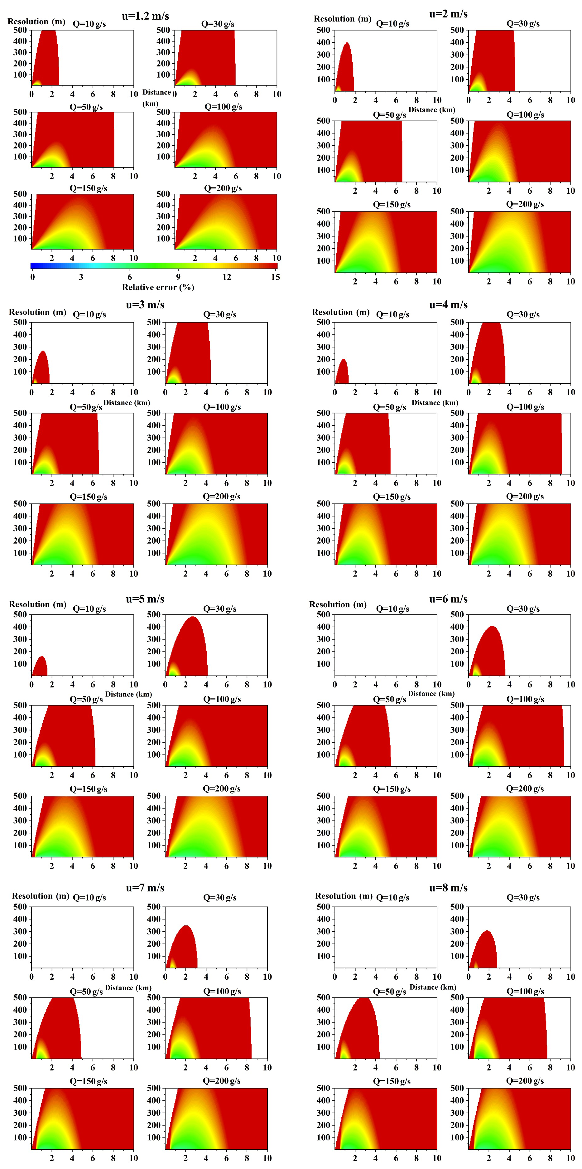
Figure A1 Relative errors (using Eq. 17) of NO_x as a function of the measurement distance from the source (x axis) and the sampling resolution (y axis). The different panels show the results for different wind speeds and different emission rates. The color map indicates the relative errors.

Appendix B: SO₂ simulation results (relative error)

Figure B1 Relative error (using Eq. 16) of the distribution of SO₂ for different wind fields of different emission rates. The unit of all abscissas is the measurement distance from the source (km), while that of the ordinate is the sampling resolution (m). The color map indicates the relative errors.