Variability of the Brunt–Väisälä frequency at the OH^∗-airglow layer height at low and midlatitudes

Airglow spectrometers, as they are operated within the Network for the Detection of Mesospheric Change (NDMC; https://ndmc.dlr.de, last access: 1 November 2020), for example, allow the derivation of rotational temperatures which are equivalent to the kinetic temperature, local thermodynamic equilibrium provided. Temperature variations at the height of the airglow layer are, amongst others, caused by gravity waves. However, airglow spectrometers do not deliver vertically resolved temperature information. This is an obstacle for the calculation of the density of gravity wave potential energy from these measurements.

As Wüst et al. (2016) showed, the density of wave potential energy can be estimated from data of OH^∗-airglow spectrometers if co-located TIMED-SABER (Thermosphere Ionosphere Mesosphere Energetics Dynamics, Sounding of the Atmosphere using Broadband Emission Radiometry) measurements are available, since they allow the calculation of the Brunt–Väisälä frequency. If co-located measurements are not available, a climatology of the Brunt–Väisälä frequency is an alternative. Based on 17 years of TIMED-SABER temperature data (2002–2018), such a climatology is provided here for the OH^∗-airglow layer height and for a latitudinal longitudinal grid of $\mathrm{10}{}^{\circ }\times \mathrm{20}{}^{\circ }$ at midlatitudes and low latitudes. Additionally, climatologies of height and thickness of the OH^∗-airglow layer are calculated.

1 Introduction

This is the succeeding publication to Wüst et al. (2017a), where the angular Brunt–Väisälä (BV) frequency was calculated for the OH^∗-layer height between 43.93–48.09^∘ N and 5.71–12.95^∘ E using Thermosphere Ionosphere Mesosphere Energetics Dynamics, Sounding of the Atmosphere using Broadband Emission Radiometry (TIMED-SABER) data from 2002 to 2015. The choice of the geographical region, which includes the Alps, was due to the location of the five Network for the Detection of Mesospheric Change (NDMC) stations: Oberpfaffenhofen (48.09^∘ N, 11.28^∘ E), the Hohenpeißenberg observatory (47.8^∘ N, 11.0^∘ E), the Environmental Research Station Schneefernerhaus (47.42^∘ N, 10.98^∘ E), Germany, and the observatories in Haute-Provence (43.93^∘ N, 5.71^∘ E), France, and Sonnblick (47.05^∘ N, 12.95^∘ E), Austria. We described seasonal variations of the three parameters, height and full width at half maximum (FWHM) of the OH^∗ layer as well as the BV frequency weighted according to the parameters of the OH^∗ layer and provided a climatology of the yearly course of this BV frequency.

Now, the data basis is extended to global TIMED-SABER measurements. Overall, 3 more years (2016–2018) are included in the analysis which changed slightly compared to Wüst et al. (2017a): instead of calculating the Gaussian-weighted BV frequency, the BV frequency is now weighted with the volume emission rate of the OH-B (1.6 µm) channel of SABER. Furthermore, the geographical position of the SABER measurements at 86 km height is taken into account (in our preceding publication, any part of the SABER profile needed to fit the geographical selection criteria).

The angular BV frequency N, which is, for example, needed for calculation of the density of gravity wave potential energy, varies with the temperature T and its vertical gradient (e.g. Andrews, 2000):

$$\begin{array}{}\text{(1)}& N\left(T,{\displaystyle \frac{\mathrm{d}T}{\mathrm{d}z}}\right)=\sqrt{{\displaystyle \frac{g}{T}}\left({\displaystyle \frac{\mathrm{d}T}{\mathrm{d}z}}-{\mathrm{\Gamma }}_{\mathrm{d}}\right)},\end{array}$$

where ${\mathrm{\Gamma }}_{\mathrm{d}}=g/c_p$ (with g equal to acceleration due to gravity, c_p the specific heat capacity of air at constant pressure) is the dry-adiabatic lapse rate defined as the vertical adiabatic temperature decrease. In most cases, its value is given as 9.8 K km⁻¹. However, the acceleration due to gravity, g, is slightly height dependent and determines together with the specific heat capacity at constant pressure, c_p, the dry-adiabatic lapse rate. g reaches a value of approximately 9.55 m s⁻² at 86 km height; therefore, the vertical adiabatic temperature decrease is approximately 9.5 K km⁻¹ there. g also depends on the geographical position due to the fact that the Earth is not a perfect sphere but oblate. Since the variation in the Earth radius is less than 86 km (only approximately one quarter of it), this effect is of minor importance and therefore neglected here.

Measurement techniques which provide vertical temperature profiles therefore allow the direct calculation of the BV frequency and of further parameters such as the density of wave potential energy (see, e.g. Kramer et al., 2015; Mzé et al., 2014; Rauthe et al., 2008, to mention just a few). OH^∗ spectrometers, however, deliver information about temperature always vertically averaged over the OH^∗ layer. OH^∗ imaging systems provide in most cases only brightness maps (e.g. Sedlak et al., 2016, and Hannawald et al., 2016, 2019, who addressed a small part of the sky, and Garcia et al., 1997, who operated an all-sky system). An exception is here Pautet et al. (2014), who worked with narrow-band filters and could derive temperature maps. At a poorer horizontal resolution scanning OH^∗ spectrometers can also deliver horizontally resolved temperature information (see, e.g. Wachter et al., 2015; Wüst et al., 2018). However, also in these cases, the temperature is vertically averaged over the OH^∗ layer; the BV frequency cannot be calculated.

So, one needs to rely on temperature climatologies or on complementary temperature measurements. The latter should be of higher accuracy in most cases, if the coincidence in time and space of the complementary and the original measurement is good enough (see Wendt et al., 2013, for the quantification of typical temperature differences due to miss time and miss distance). Since complementary measurements are rare and not available at every NDMC station and at every time, a climatology of the BV frequency based on global satellite-based measurements is very valuable. Approximately 85 % of all spectrometers and photometers listed in the database of NDMC address at least one of the various OH emissions (Schmidt et al., 2018); thus, TIMED-SABER OH-B channel and temperature measurements are used for the BV frequency climatology. The OH-B channel covers the wavelength range from 1.56 to 1.72 µm, which includes mostly the OH (4-2) and OH (5-3) vibrational transition bands. The peak altitude difference for adjacent vibrational levels is approximately 500 m (e.g. Adler-Golden, 1997; von Savigny et al., 2012) and therefore negligible compared to the FWHM, which is typically cited to be 8.6 km±3.1 km (Baker and Stair, 1988). Of course, a climatology based on global satellite measurements always provides averaged information. Effects of processes which vary during one night, such as gravity waves, or those which change significantly from year to year are not (or only to a small extent) included (due to the thickness of the OH^∗ layer, at least small-scale variations cancel out; see, e.g. Wüst et al., 2016). Especially tides can affect the BV frequency significantly since they are able to change the temperature and also the temperature gradient. Mukhtarov et al. (2009) showed, for example, that the amplitude of the diurnal migrating (meaning Sun-synchronous) tide varies during the year but maximizes at the equatorial mesosphere with amplitudes of 19 K at 90 km height. The amplitude is lower at midlatitudes. The vertical wavelength in this height range is approximately 20 km. The amplitude of the semi-diurnal migrating tide shows another latitudinal structure at 90 km height with maxima of approximately 9 K, which are reached around 40^∘ N/S (Pancheva et al., 2009). The vertical wavelengths are larger in summer (∼38–50 km) than in winter (∼25–35 km). These results concern tides propagating to the west. The eastward-propagating diurnal and semi-diurnal tides are, for example, investigated in Pancheva et al. (2010a). They are characterized by smaller amplitudes. Therefore, we additionally provide an uncertainty range of the BV frequency due to tides in this publication.

2 Data and analysis

We use TIMED-SABER temperature and OH-B channel data (volume emission rate; VER) in version 2.0 for the years 2002 to 2018. It was downloaded from the SABER homepage (http://saber.gats-inc.com/, last access: 6 December 2019). In order not to duplicate information, the reader is referred to our preceding publication (Wüst et al., 2017a) and publications therein for more details about TIMED-SABER (Mertens et al., 2004; Mlynczak, 1997; Russell et al., 1999), the retrieval of kinetic temperatures (Dawkins et al., 2018; Garcia-Comas et al., 2008; López-Puertas et al., 2004; Mertens et al., 2004, 2008; Remsberg et al., 2008) and a comparison between SABER v2.0 temperature and ground-based lidar data (Dawkins et al., 2018). Since the OH^∗ spectrometers only allow measurements during nighttime, we calculate the exact local time (by adding 4 min to UTC for every longitudinal degree) and require SABER measurements between 18:00 and 06:00 LT (local time).

The squared BV frequency $N_i^{\mathrm{2}}$ is computed for each SABER profile at every available height and weighted with the OH VER. The result is called the OH^∗-equivalent BV frequency in the following. From time to time, a maximum in the VER is observed around 40 km height and the respective profile shows strong oscillations. These profiles are excluded from further analysis steps.

Furthermore, information about the OH^∗ layer is derived from the OH VER profiles. The centroid height is denoted as the OH^∗ height in the following and the FWHM is calculated by determining the maximum of the OH VER and subtracting the lower height from the upper height where half of the maximum is reached for the first time (starting at the height of maximal OH VER).

In the following, the OH^∗ height, the FWHM and the OH^∗-equivalent BV frequency are mapped to a $\mathrm{20}{}^{\circ }\left(\text{longitude}\right)\times \mathrm{10}{}^{\circ }\left(\text{latitude}\right)$ grid. The data are ascribed to the midpoints of the respective intervals. Here, the geographical position of the SABER measurement at 86 km height is taken into account. Then, the daily mean of each parameter is calculated for every grid cell. This is done for all years. It is assumed that every year is a leap year; this facilitates further calculations.

Due to the yaw cycle of SABER, data gaps are visible at higher latitudes and all investigations in this publication include the latitudinal range of 52^∘ S to 52^∘ N.

3 Results and discussion

All three parameters (the OH^∗-layer height, the FWHM and the OH^∗-equivalent BV frequency) vary with latitude, longitude, day of year (DoY) and local time. In this section, the results will be first described qualitatively based on some examples. Then, the annual development of the OH^∗-equivalent BV frequency will be approximated and the respective mathematical function will be provided.

3.1 Variations of OH^∗ height, FWHM and OH^∗-equivalent BV frequency

Since the BV frequency depends on temperature, which changes strongly with DoY and latitude, one would expect that the BV frequency varies more with these two parameters than with longitude. Both the latitudinal and the temporal dependence of the temperature are strongly determined by the residual circulation (see, e.g. Garcia and Solomon, 1985, who give a concise overview in their introduction about the development of our knowledge concerning the mean meridional circulation). The residual circulation consists of horizontal and vertical movements. The higher the latitude, the more important the vertical movement and the less important the horizontal one becomes. The vertical movement influences the temperature through adiabatic warming or cooling but also the downward transport of atomic oxygen (the dominating species for the formation of OH^∗) from heights above the OH^∗ layer and therefore the OH^∗ height and thickness (e.g. Shepherd et al., 2006): a downward movement leads to a lower and brighter OH^∗ layer, and vice versa. On average, the OH^∗ layer is thicker (thinner) during a prevailing downward (upward) movement (e.g. Liu and Shepherd, 2006). Therefore, it is not surprising that an annual cycle is clearly visible in the temporal development of all three parameters at midlatitudes. It dominates the development of the OH^∗ height and the OH^∗-equivalent BV frequency during the year at all longitudes for 45^∘ N (Fig. 1a), for example. The FWHM additionally shows a period of approximately 60 d in every season but summer. At low latitudes, the annual cycle is less pronounced. At all longitudes for 5^∘ N, for example, a semi-annual cycle and superimposed oscillations with smaller periods of approximately 60 d (especially for the FWHM and the OH^∗-equivalent BV frequency) gain importance for the development of the three parameters during the year or even dominate it (Fig. 1b).

Figure 1 OH^∗-layer height (a, d), FWHM (b, e) and OH^∗-equivalent BV frequency (c, f) are shown for the latitudinal band of $\mathrm{45}\pm \mathrm{5}{}^{\circ }$ N (a–c) and $\mathrm{5}\pm \mathrm{5}{}^{\circ }$ N (d–f) depending on longitudinal bands (longitude $\pm \mathrm{10}{}^{\circ }$, colour coded) and DoY. The data are averaged for each DoY. Additionally, they are subject to a 31-point sliding mean. In order to facilitate comparison, the scales of the plots referring to $\mathrm{45}\pm \mathrm{5}{}^{\circ }$ N and $\mathrm{5}\pm \mathrm{5}{}^{\circ }$ N are identical.

The annual development of the OH^∗-layer height, the FWHM and the OH^∗-equivalent BV frequency varies to some extent also with longitude. For the different longitudes, the yearly latitudinal means over the three parameters range between approximately 85 and 87 km, 7.0 and 8.25 km, and 0.020 and 0.023 s⁻¹ (Fig. 2). The longitudinal variability (peak-to-peak difference) is at maximum approximately 1.5 km (approximately 2 % relative to 86 km) for the OH^∗-layer height, approximately 1 km (approximately 13 % relative to 7.6 km) for the FWHM and approximately 0.001 s⁻¹ (approximately 5 % relative to 0.0215 s⁻¹) for the OH^∗-equivalent BV frequency (Fig. 2). The graphs referring to the different longitudes spread more for 5^∘ N than for 45^∘ N (Fig. 1).

Figure 2 OH^∗-layer height (a), FWHM (b) and OH^∗-equivalent BV frequency (c) are averaged over all years and plotted for the latitudinal bands $\mathrm{45}\pm \mathrm{5}{}^{\circ }$ S to $\mathrm{45}\pm \mathrm{5}{}^{\circ }$ N, 50–52^∘ N/S (colour coded). Please be aware that the axes of the respective plots of Figs. 1 and 2 are not identical.

Therefore, the approximation of the annual development of the OH^∗-equivalent BV frequency will be calculated on a latitude–longitude grid, which is $\mathrm{10}{}^{\circ }\times \mathrm{20}{}^{\circ }$. The number of values per grid cell and year varies strongly. For high latitudes (53^∘ N or ^∘ S and more), the OH^∗-equivalent BV frequency can be provided for half a year and less due to the TIMED yaw cycle. Thus, these latitudes are excluded from further investigations. For midlatitudes and low latitudes, data gaps exist only for individual days. For the climatology of the OH^∗-equivalent BV frequency, which is based on 17 years of TIMED-SABER data, approximately 80–190 values are available per grid cell and day at maximum. The number of values and the variation in the number of values per grid cell over the year is higher for midlatitudes compared to low ones. The average number of values per grid cell and day ranges between approximately 45 (for low latitudes) and 85 (for midlatitudes).

3.2 Possible reasons for the variations of the OH^∗ height, the FWHM and the OH^∗-equivalent BV frequency

In the following, we discuss the possible origin of the oscillations described above. Here, we have to discriminate between natural phenomena and possible artefacts due to the yaw cycle of TIMED in order to chose a correct mathematical approximation of the annual development of the BV frequency.

3.2.1 The 60 d oscillation

The overpass time of TIMED-SABER varies with DoY (Fig. 3, only nightly overpasses considered): TIMED flies by a little bit earlier every day with respect to a fixed geographical position and has a yaw cycle of 60 d, i.e. the viewing direction of the instrument changes every 60 d, and the overpass time at a specific geographical position is the same every 120 d for the same viewing direction (ascending or descending part of the orbit). If the observed parameter has a fixed daily cycle, an artificial 120 d oscillation can be generated in the respective time series. Zhang et al. (2006) showed such a periodicity in SABER temperature measurements at 86 km height in their Fig. 2a. If the viewing direction is neglected, the overpass time is identical every 60 d. In this case, an artificial 60 d oscillation could be generated in the respective time series.

Figure 3 Local overpass time of TIMED for the grid cells at 5^∘ N, 10^∘ E (dark grey), and 45^∘ N, 10^∘ E (light grey), for the year 2002 between 18:00 and 06:00 LT. A negative local time means that the respective profile was recorded before midnight (−2 LT = 22:00 LT, −4 LT = 20:00 LT, −6 LT = 18:00 LT). Daily averages are not computed; this plot shows the individual measurements (959 for 5^∘ N and 1626 for 45^∘ N).

The BV frequency depends not only on temperature but also on the vertical temperature gradient. Changes in temperature and its vertical gradient can affect the development of the BV frequency during the night but they do not necessarily need to (if both temperature and vertical temperature gradient, increase (or decrease) simultaneously, their effect on the BV frequency can also cancel out; see Eq. 1). Approximating linearly the temporal dependence of temperature and its vertical gradient during nighttime for 5^∘ N gives −0.94 K h⁻¹ and −0.25 K km⁻¹ h⁻¹ (Fig. 4a and b; the squared correlation coefficient R² is 6 % and 17 %). For 45^∘ N, the parameters increase on average by 0.81 K h⁻¹ and 0.04 K km⁻¹ h⁻¹ during the night (Fig. 4c and d; R² is 3 % and 0.4 %). Assuming a linear behaviour of both the temperature and its vertical gradient, an effect on the BV frequency cannot be derived for 45^∘ N. For 5^∘ N, the BV frequency shows a temporal dependence (Fig. 4e), which is the condition for a sensitivity to the yaw cycle. Even though the respective R² values are very low, the result is consistent with our observations (Fig. 1c and f).

Figure 4 Temperature and vertical temperature gradient, both VER weighted, for 5^∘ N (a, b) and 45^∘ N (c, d) for the year 2002. The nomenclature concerning the local time agrees with the one explained in the caption of Fig. 3. Panel (e) shows the development of the BV frequency during the night for 5^∘ N, 10^∘ E (black), and 45^∘ N, 10^∘ E (grey), based on the linear approximation of temperature and its vertical gradient.

Let us have a closer look on the variability of temperature and its vertical gradient during night. During one night, both parameters are influenced amongst others by tides. As shown by Pancheva et al. (2009) and Mukhtarov et al. (2009) based on 5 years of TIMED-SABER observations, the amplitude of the diurnal and semi-diurnal tide varies from month to month and so does their influence on the BV frequency. From April to July, the amplitudes of both tides show a common minimum at 90 km height and 40^∘ N, whereas the diurnal tide is maximal in February and March as well as in August and September. The semi-diurnal tide reaches its highest amplitudes from November to February. These results are supported by Silber et al. (2017), who show in their Fig. 7 that tidal amplitudes in general are relatively low during summer for 4 years of GRIPS (Ground-based Infrared P-branch Spectrometer) data in Tel Aviv (32.1^∘ N, 34.8^∘ E). Also the phases of the diurnal and semi-diurnal tides vary to some extent (see again Pancheva et al., 2009, and Mukhtarov et al., 2009, for measurements between 50^∘ S and 50^∘ N). Silber et al. (2017) depict in their Fig. 9 that the phases of the diurnal and the semi-diurnal tide are at least over some time relatively stable (the tides are approximated by a cosine starting at 12:00 LT; the phases approach values near zero on average).

A nearly linear relation between observation time and temperature (vertical temperature gradient) can only be expected if the diurnal tide dominates over the semi-diurnal and its phase is 06:00 or 18:00 LT (00:00 or 12:00 LT) in the case that the tide is approximated by a cosine. The weighting with VER smears the signals. Temperature and temperature gradient should show different variations during the year due to tides. The low amplitudes during summer are captured by the strength of the 60 d oscillation in the OH^∗-equivalent BV frequency time series.

These effects probably explain the low R² values and lead to the large spread around the linear regression shown in Fig. 4a–d.

Tidal influence could also explain the oscillation of approximately 60 d in the FWHM at 45^∘ N during parts of the year. Compared to the calculation of the OH^∗-layer height and of the BV frequency, the FWHM is not weighted by the VER (see Sect. 2), and therefore it is more sensitive to individual variations of the OH VER profile. Amongst others, these individual variations are due to tides which systematically influence the temperature and its gradient but also the downward mixing of atomic oxygen. Only during selected time intervals (e.g. approximately DoY 90–120, 220–250 and 330–365; see Fig. 3) are profiles sensed at different times of the night (time difference of approximately 4 h) available. Comparing Figs. 3 and 1b, one can see, for example, around DoY 30–40 that the gradient of the FWHM changes its sign when the observation time jumps in this case from approximately 18:00 to 06:00 LT.

However, oscillations with slightly shorter periods than 60 d (approximately 50 d) are also observed in measurements which are not affected by a 60 d yaw cycle as, for example, Rüfenacht et al. (2016) showed based on horizontal wind values derived from a ground-based Doppler wind radiometer. Those measurements refer to the altitude range between the mid-stratosphere (5 hPa) and the upper mesosphere (0.02 hPa); low, middle and high latitudes are addressed in the publication. The observed periods between 20 and 50 d are subject to temporal variations. The reason for these oscillations is not clear. The authors discuss a link to solar forcing; however, they point out that solar forcing might influence the atmospheric wave pattern only in an indirect way. Therefore, it is possible that we see a mixture of natural and artificial effects in our data. However, we cannot distinguish between them and ignore the 60 d oscillation for our BV climatology.

Comparing the large-scale dynamics (tides and planetary waves) of low and midlatitudes, there are prominent differences. Offermann et al. (2009) showed in their Fig. 8 that tidal motions in general gain more and more importance in comparison to planetary waves at approximately 90 km height the lower the latitude is. At 20^∘ N, tidal waves cause more variability than stationary planetary waves. Compared to travelling planetary waves, tidal variations lie in the same range (Offermann et al., 2009). We can conclude that at low latitudes the effect of tidal motions on temperature is at least of the same order of magnitude as the influence of planetary waves.

Concerning the temperature gradient, we can argue as follows: the influence of waves on the temperature gradient depends on the vertical wavelength (the larger the wavelength, the smaller the influence of waves with the same amplitude) and the amplitude of the wave (the larger the amplitude, the greater the influence of waves with the same vertical wavelength). The vertical phase velocity determines how fast the influence is changing. The mean vertical wavelength of the 5 d Rossby wave, for example, is approximately 50–60 km according to Pancheva et al. (2010b), who investigated TIMED-SABER temperature measurements for 6 full years from January 2002 to December 2007, while the vertical wavelengths of tides are mostly in the same range or slightly smaller and reach approximately 30 km at minimum as, for example, Zhang et al. (2006) showed for case studies and Forbes et al. (2008), who used TIMED-SABER temperature measurements from March 2002 to December 2006. Additionally, the periods of tides are smaller compared to planetary wave periods; tides have a larger vertical phase velocity. That means that at low latitudes, tides influence the temperature gradient and its change during night stronger than planetary waves. This agrees qualitatively with the results shown in Fig. 4.

3.2.2 Annual and semi-annual variation

As mentioned above, visual inspection of Fig. 1 depicts at least one additional oscillation with a semi-annual period besides the annual cycle and the 60 d variation. Semi- and even ter-annual periods are observed by other authors and in different parameters (for the semi-annual cycle in different parameters in the mesosphere and higher but not specifically for airglow, see, e.g. the introduction of Silber et al., 2016). Based on WINDII (Wind Imaging Interferometer) measurements between 60^∘ N and 60^∘ S from 1991 to 1997, Shepherd et al. (2006) showed in their Fig. 1 a semi-annual variation in the OH emission rate between approximately 20^∘ N and 20^∘ S with maxima in spring and autumn. The authors attribute this oscillation to the semi-annual variation of the downward mixing associated with the variation in amplitude of the diurnal tide. Liu and Shepherd (2006) pointed out that the column-integrated emission rate is inversely related to the peak height for WINDII data between 40^∘ S and 40^∘ N, and developed an empirical model for predicting the altitude of the peak of the OH nightglow emission. Here, they included amongst others sinusoidal annual and semi-annual variations. Mulligan et al. (2009) transferred this model to Longyearbyen (78^∘ N, 16^∘ E) and found amplitudes unequal to zero for the annual and semi-annual modes. For low latitudes, von Savigny (2015) showed minima in the OH^∗ height in spring and autumn. Annual, semi- and ter-annual oscillations are also observed in temperature: as published by Höppner and Bittner (2007) in their Fig. 2 for Wuppertal, Germany (51^∘ N, 7^∘ E), in 1993, the OH^∗ temperature derived by the ground-based GRIPS does not show just an annual cycle; it is characterized by a kind of plateau at DoY 40–80 (February and March) and DoY 260–300 (September and October). Therefore, the authors approximate the overall yearly course as (quasi) annual, (quasi) semi-annual and (quasi) ter-annual sinusoidal (see also Bittner et al., 2000, 2002). Those plateaus can also be observed using GRIPS data at other stations, e.g. in Tel Aviv (see Wüst et al., 2017b), and if the temperature data are averaged over some years (tested for the Environmental Research Station Schneefernerhaus (UFS) and not shown here).

3.3 Approximation of the OH^∗-equivalent BV frequency

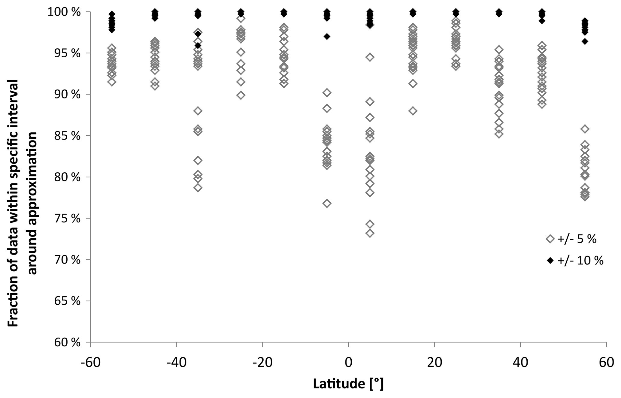
In order to provide qualitative results, the harmonic analysis (one-step mode; see, e.g. Wüst and Bittner, 2006) is applied to the time series of OH^∗-equivalent BV frequency averaged over each DoY and separated according to latitude and longitude. In order to avoid the approximation of the 60 d oscillation, which might be due to sampling tides at different phases as discussed above, the period range which the harmonic analysis uses is restricted to 180–366 d. That means tidal effects are not included here. The number of oscillations is chosen to be two. The results are summarized in Table 1, and two examples for the approximation are shown in Fig. 5. The quality of approximation (that means $\mathrm{1}-{\mathit{\sigma }}_{\mathrm{res}}^{\mathrm{2}}/{\mathit{\sigma }}^{\mathrm{2}}$, where σ² is the variance of the original time series and ${\mathit{\sigma }}_{\mathrm{res}}^{\mathrm{2}}$ is the variance of the residual time series, so the original time series minus the approximation) is plotted versus latitude in Fig. 6. In most cases, the two oscillations show periods in the range of an annual and semi-annual cycle. As already mentioned above, using the latitudes of 5^∘ N and 45^∘ N, the importance of the 60 d oscillation, which is not adapted, increases with decreasing latitude. Therefore, the quality of approximation over all longitudes reaches its minimum near the Equator (Fig. 6). The asymmetry in the quality of approximation between the Northern Hemisphere and the Southern Hemisphere is remarkable. This agrees quite well with asymmetries in tidal activity observed, for example, by Vincent et al. (1989). Those authors investigated radar wind observations which refer to 80–100 km height in Adelaide (35^∘ S, 138^∘ E) and Kyoto (35^∘ N, 136^∘ E), two places which are symmetrically located around the Equator. The diurnal tidal winds in Adelaide have a larger amplitude than in Kyoto (factor 2–3). However, the reason for this behaviour is not entirely clarified. There exist hemispheric differences in tidal forcing but also differences in the middle atmosphere winds through which the tides must propagate and finally differences in dissipation. Concerning the amplitudes of the semi-diurnal tide, the authors found out that they are in general smaller at both sites than the amplitudes of the diurnal tide. During local summer, the amplitudes are larger in Adelaide. For many latitudes, longitudinal differences are clearly visible in the quality of approximation. However, when taking a ±10 % interval around the approximation, all data are covered in nearly all cases (Fig. 7).

Table 1 Period (T), amplitude (A) and phase (φ) of the two oscillations which explain the variability of the daily OH^∗-equivalent BV frequency values (averaged over all years) best for a latitudinal and longitudinal gridding of 10^∘ and 20^∘. They oscillate around the respective mean. The OH^∗-equivalent BV frequency (s⁻¹) can be estimated by the $\text{mean}+{\sum }_{i=\mathrm{1}}^{\mathrm{2}}{A}_i\sin \left(\frac{\mathrm{2}\mathit{\pi }}{T_i}\cdot \text{DoY}-{\mathit{\phi }}_i\right)$. Due to leap years, the total amount of days for 1 year is set to 366, which means 1 March is DoY 61 for every year. The harmonic oscillation explains the variability in the time series of daily OH^∗-equivalent BV frequency values to a different extent. The respective value is provided in the column “quality of approximation”. Additionally, the fraction of data which lies within intervals of ±5 % or ± 10 % around the harmonic approximation is given.

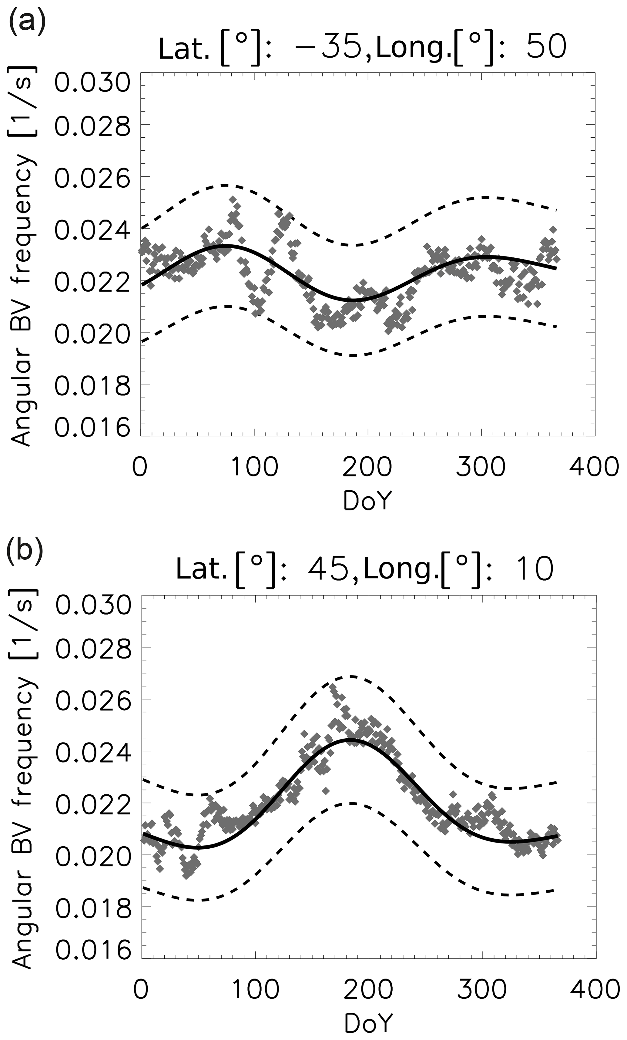
Figure 5 Comparison of the approximation of the BV frequency (solid line) with the approximated values for two different bins. The dashed line refers to the ±10 % interval around the approximation.

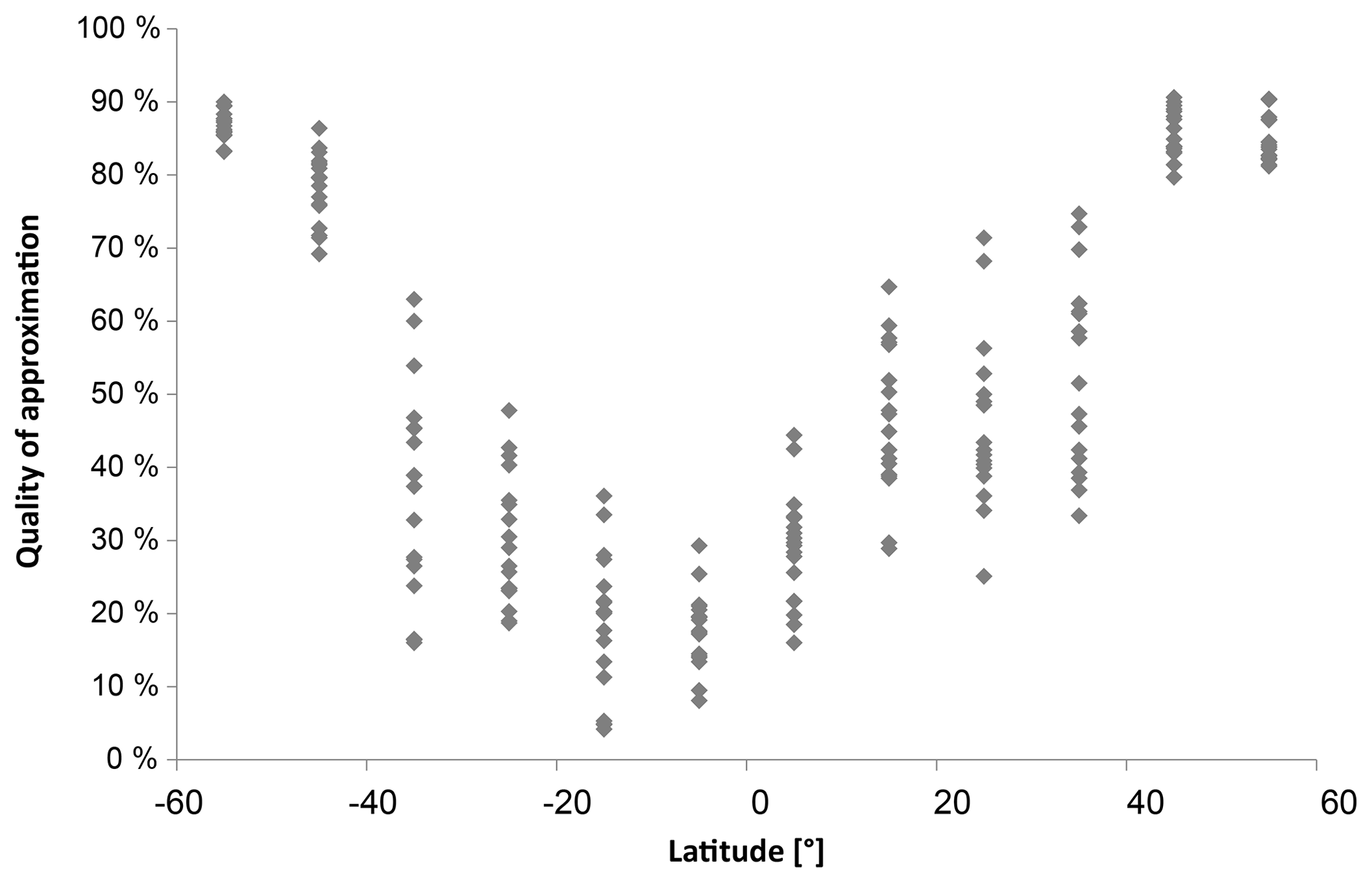
Figure 6 Quality of approximation as shown in Table 1 versus latitude. All longitudes are plotted but not separated by colour in order to keep the figure clear.

Figure 7 Fraction of data within ±5 % and ±10 % intervals around the approximation.

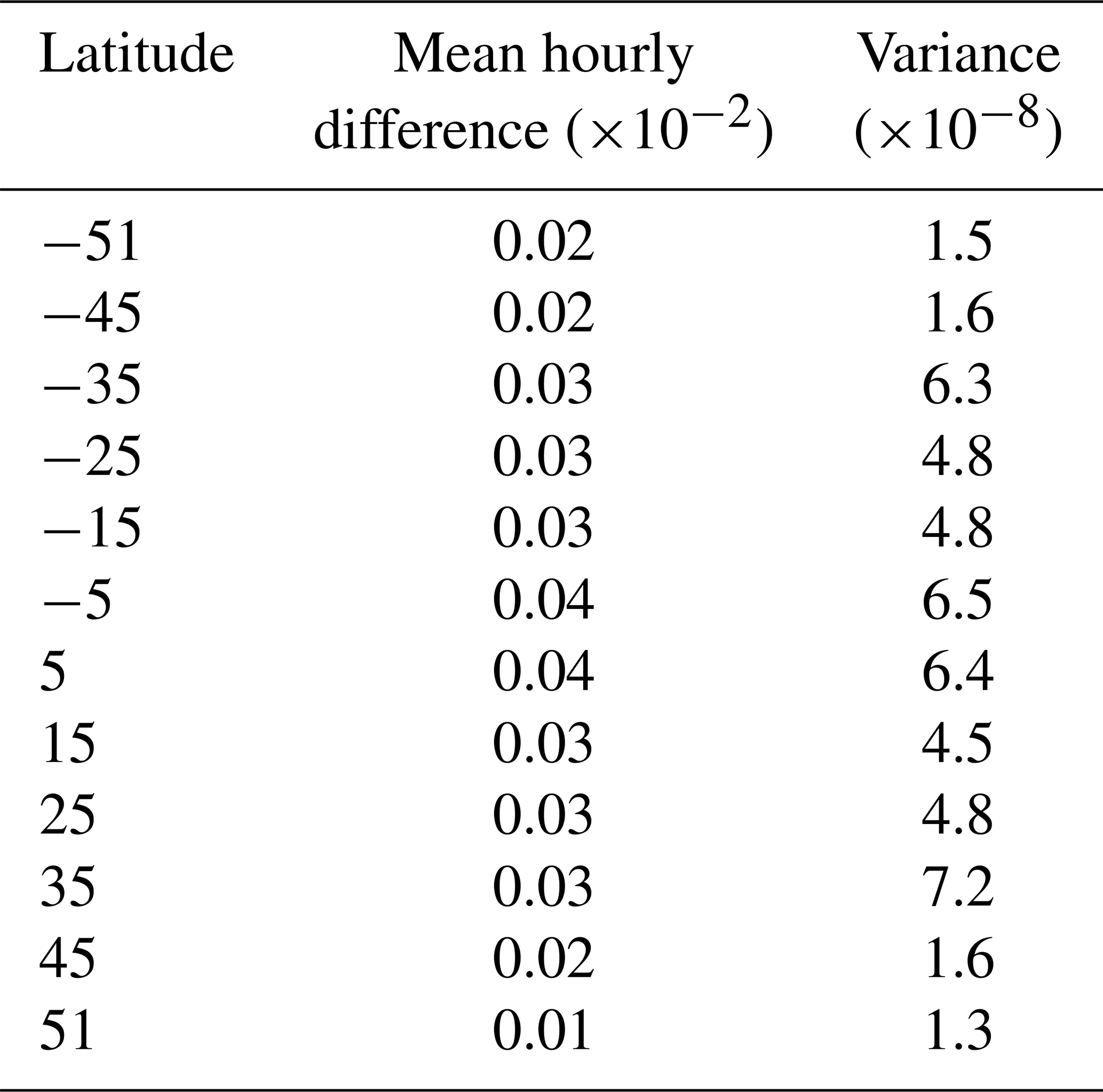
As mentioned above, tidal effects are not included in the approximation of the OH^∗-equivalent BV frequency. However, an uncertainty range of the OH^∗-equivalent BV frequency due to these effects is additional useful information. In order to estimate it, SABER profiles which refer to the same night (between 18:00 and 06:00 LT) and are separated by 6 h at minimum are collected for all years (2002–2018) at each grid point. Since tides have periods in the range of 6 h and more (the dominating ones have periods of 12 and 24 h), we argue that the difference of the OH^∗-equivalent BV frequency within these hours during one night is mainly due to tides. Of course, also gravity waves still play a role in this period range. Since our gridding is relatively coarse for gravity waves, we assume that gravity waves increase and decrease the OH^∗-equivalent BV frequency in one pixel so that their effect cancels out over time. This is not true for larger-scale phenomena. The mean difference per hour over all years is calculated at each grid point. The results are averaged over latitude afterwards (Table 2). The amount of data per latitude measurement is on the order of magnitude of 10 000. As mentioned above, tidal activity varies during the year. Therefore, the provision of monthly values would make more sense. However, especially at midlatitudes and high latitudes, SABER profiles which refer to the same night separated by 6 h at least are not evenly distributed over the year or not available every month. The uncertainty range provided in Table 2 can therefore be regarded as a rather rough estimate. With respect to an OH^∗-equivalent BV frequency of 0.02 s⁻¹, the results are in the range of approximately 1 %–2 %. For a night of 12 h, tidal effects sum up to approximately 21 % at maximum (meaning for low latitudes). We can assume that the approximation of the OH^∗-equivalent BV frequency refers to midnight, so the tidal effects can be approximated by ±11 % for the whole night in this case.

Table 2 Shown are the mean difference per hour and its variance for the OH^∗-equivalent BV frequency measured during the same night for the different latitudinal intervals ($-\mathrm{45}\pm \mathrm{5}{}^{\circ }$ until $+\mathrm{45}\pm \mathrm{5}{}^{\circ }$, $-\mathrm{51}\pm \mathrm{1}{}^{\circ }$ and $+\mathrm{51}\pm \mathrm{1}{}^{\circ }$).

As mentioned at the beginning, this is the succeeding paper to Wüst et al. (2017a) where the authors proposed an approximation of the OH^∗-equivalent BV frequency for the Alpine region more exactly for 43.93–48.09^∘ N and 5.71–12.95^∘ E based on three oscillations. The question, which naturally arises now, is how the two different approximations, the one of Wüst et al. (2017a) and one proposed here, compare. The following differences exist in methods and data basis: the pixel size of Wüst et al. (2017a) is approximately $\mathrm{5}{}^{\circ }\times \mathrm{7}{}^{\circ }$ and therefore less than 25 % of the pixel size applied here. Wüst et al. (2017a) use three oscillations and SABER data from 2002 to 2015; we use two oscillations and SABER data from 2002 to 2018. Furthermore, instead of calculating the Gaussian-weighted BV frequency, the OH^∗-equivalent BV frequency is now weighted with the volume emission rate of the OH-B channel of SABER. Then, the geographical position of the SABER measurements at 86 km height is taken into account (in our preceding publication, any part of the SABER profile needed to fit the geographical selection criteria). Finally, the dry-adiabatic lapse rate is assumed to be 9.8 K km⁻¹ in Wüst et al. (2017a); now, it is 9.5 K km⁻¹ since the height dependence of g is taken into account here. As Fig. 8 shows, the two approximations agree for the majority of the year within an uncertainty of 5 %. This is in the range of the natural variability (see Table 1). There is an offset visible, which is due to the height dependence of the dry-adiabatic lapse rate. Furthermore, the data disagree especially where the ter-annual oscillation used by Wüst et al. (2017a) has a maximum. This oscillation is not used here since tests showed that it appears very prominently at low latitudes in order to approximate at least in part the oscillation of approximately 60 d. Even though temperature data at midlatitudes also show a slight ter-annual course as discussed above, it is not clear until which latitude the ter-annual oscillation might be real and from which latitude on it might be artificial. Therefore, we propose to use the values of Wüst et al. (2017a) for investigations which do not comprise a direct comparison with results from stations not within 43.93–48.09^∘ N and 5.71–12.95^∘ E. In any other case, the values of this paper should be applied.

Figure 8 Comparison of the approximation of the BV frequency in the Alpine region as it was proposed by Wüst et al. (2017a) based on three oscillations (black) and in this paper (grey, values of the pixel at 45^∘ N and 10^∘ E are used).

Even though a climatology of the OH^∗-layer height and its FWHM is not in the focus of this paper, it might be of interest for some scientific groups. Therefore, the harmonic analysis is applied to the time series of daily mean values of the OH^∗-layer height and of the FWHM in the same way as it was used for the approximation of the BV frequency. The results are listed in Tables A1 and A2.

4 Summary and outlook

We provide a climatology of the OH^∗-equivalent BV frequency based on 17 years of TIMED-SABER data for midlatitudes and low latitudes on a $\mathrm{10}{}^{\circ }\times \mathrm{20}{}^{\circ }$ grid. This is done in order to facilitate the estimation of the density of gravity wave potential energy from airglow temperature measurements independent of co-located measurements which deliver vertical temperature profiles. This paper is the succeeding work of Wüst et al. (2017a), who published a climatology for the Alpine region only.

Especially at low latitudes, a prominent 60 d oscillation is present in the time series of daily OH^∗-equivalent BV frequency averaged over all years. This might be an artificial signal due to a combination of the yaw cycle of SABER and strong tidal activity. Physical reasons for the annual and semi-annual oscillations, which are also present in the data, are known. Therefore, an analytical formulation for the approximation of the daily OH^∗-equivalent BV frequency based on the superposition of a mean value and two further oscillations (in most cases a nearly annual and a nearly semi-annual) is provided. It is estimated based on a harmonic analysis approach, and the approximation is usually better than ±10 %. An uncertainty range for tidal influences during one night is calculated, which indicates that in the tropics sometimes uncertainties of up to ±11 % can occur. An improvement over our previous work is that additional formulations for daily values of the OH^∗-layer height and thickness are also given.

Appendix A

Table A1 Same as Table 1 but for the OH^∗-layer height. Please note that OH^∗-layer height is less variable during the year, and therefore the fraction of data around the approximation is provided for intervals of ±1 % and ±2 %.

Table A2 Same as Table 1 but for the FWHM. Please note that FWHM is more variable during the year, and therefore the fraction of data around the approximation is provided for intervals of ±7.5 % and ±15 %.