Version 2 Ozone Monitoring Instrument SO₂ product (OMSO2 V2): new anthropogenic SO₂ vertical column density dataset

The Ozone Monitoring Instrument (OMI) has been providing global observations of SO₂ pollution since 2004. Here we introduce the new anthropogenic SO₂ vertical column density (VCD) dataset in the version 2 OMI SO₂ product (OMSO2 V2). As with the previous version (OMSO2 V1.3), the new dataset is generated with an algorithm based on principal component analysis of OMI radiances but features several updates. The most important among those is the use of expanded lookup tables and model a priori profiles to estimate SO₂ Jacobians for individual OMI pixels, in order to better characterize pixel-to-pixel variations in SO₂ sensitivity including over snow and ice. Additionally, new data screening and spectral fitting schemes have been implemented to improve the quality of the spectral fit. As compared with the planetary boundary layer SO₂ dataset in OMSO2 V1.3, the new dataset has substantially better data quality, especially over areas that are relatively clean or affected by the South Atlantic Anomaly. The updated retrievals over snow/ice yield more realistic seasonal changes in SO₂ at high latitudes and offer enhanced sensitivity to sources during wintertime. An error analysis has been conducted to assess uncertainties in SO₂ VCDs from both the spectral fit and Jacobian calculations. The uncertainties from spectral fitting are reflected in SO₂ slant column densities (SCDs) and largely depend on the signal-to-noise ratio of the measured radiances, as implied by the generally smaller SCD uncertainties over clouds or for smaller solar zenith angles. The SCD uncertainties for individual pixels are estimated to be ∼ 0.15–0.3 DU (Dobson units) between ∼ 40^∘ S and ∼ 40^∘ N and to be ∼ 0.2–0.5 DU at higher latitudes. The uncertainties from the Jacobians are approximately ∼ 50 %–100 % over polluted areas and are primarily attributed to errors in SO₂ a priori profiles and cloud pressures, as well as the lack of explicit treatment for aerosols. Finally, the daily mean and median SCDs over the presumably SO₂-free equatorial east Pacific have increased by only ∼ 0.0035 DU and ∼ 0.003 DU respectively over the entire 15-year OMI record, while the standard deviation of SCDs has grown by only ∼ 0.02 DU or ∼ 10%. Such remarkable long-term stability makes the new dataset particularly suitable for detecting regional changes in SO₂ pollution.

1 Introduction

Despite substantial overall downward trends in recent years (e.g., Aas et al., 2019; Klimont et al., 2013), sulfur dioxide (SO₂) emitted from anthropogenic sources (e.g., coal-fired power plants) continues to have significant impacts on the environment (Seinfeld and Pandis, 2006). SO₂ is toxic and a regulated criteria air pollutant in many countries (e.g., U.S. Environmental Protection Agency, 2010). It is also a precursor to secondary sulfate aerosols that contribute to smog and haze (e.g., Huang et al., 2014), cause acid deposition (e.g., Likens et al., 1996), and influence regional climate (e.g., Chuang et al., 1997; Haywood and Boucher, 2000). Removal of SO₂ and other short-lived pollutants is expected to bring health benefits (Lelieveld et al., 2019) but may also lead to additional warming (Samset et al., 2018). The ability to monitor global and regional changes in SO₂ pollution is thus critical for predicting and mitigating both air pollution and climate change.

Since the 1990s, a series of hyperspectral satellite sensors that measure solar backscattered radiances in the ultraviolet (UV) spectral range of ∼ 300–400 nm has provided global monitoring of anthropogenic SO₂ (e.g., Eisinger and Burrows, 1998; Lee et al., 2008; Nowlan et al., 2011; Theys et al., 2017; Valks and Loyola, 2008; Yang et al., 2013; Zhang et al., 2017). Among these sensors, the Ozone Monitoring Instrument (OMI) aboard the NASA Earth Observing System Aura spacecraft (Levelt et al., 2006) is particularly useful for SO₂ observations, thanks to its high spatial resolution (best at its launch in 2004) and daily contiguous global coverage. The 15-year and growing OMI SO₂ data record is the longest among those from similar UV backscatter instruments (Levelt et al., 2018), having facilitated a number of studies on regional trends of SO₂ pollution. For example, OMI data have provided observational evidence on the efficacy of SO₂ control measures in China (Li et al., 2010; 2017a), confirmed significant further reductions in SO₂ emissions from the United States (Fioletov et al., 2011; He et al., 2016) and Europe (Krotkov et al., 2016), and detected large recent increases in SO₂ pollution over India (e.g., Li et al., 2017a; Lu et al., 2013). OMI SO₂ data have also helped to quantify emissions from different types of sources (e.g., Carn et al., 2017; Fioletov et al., 2016; Kharol et al., 2020; Zhang et al., 2019), to identify sources that are missing or underestimated in bottom-up emission inventories (McLinden et al., 2016), and to build a hybrid SO₂ inventory that combines both top-down and bottom-up emission estimates (Liu et al., 2018). More recently, OMI SO₂ data have been used to study changes in acid deposition over the eastern United States (Fedkin et al., 2019) and China (Zhang et al., 2020).

Several different techniques have been applied to OMI SO₂ retrievals. The first-generation OMI standard SO₂ total vertical column density (VCD) product (OMSO2 V1.1 and earlier versions; see Table 1 for a summary of different versions of OMSO2 product) is based on the band residual difference (BRD) algorithm (Krotkov et al., 2006) for planetary boundary layer (PBL) SO₂ VCDs (primarily for monitoring anthropogenic pollution) and the linear fit (LF) algorithm (Yang et al., 2007) for volcanic SO₂ VCDs. Both are discrete wavelength algorithms that only use a small subset of OMI wavelengths in the spectral range of interest. They are fast and sensitive to sources such as large power plants and degassing volcanoes but are relatively noisy and are prone to artifacts. Starting from OMSO2 V1.2, a new retrieval technique based on principal component analysis (PCA) of OMI-measured radiances (Li et al., 2013) was introduced to produce the OMI PBL SO₂ dataset. The PCA-based spectral fitting algorithm makes use of all available OMI wavelengths between 310.5 and 340 nm, suppressing retrieval noise by a factor of 2 as compared with the BRD algorithm and largely eliminating unphysical biases over clean background areas. These improvements allow SO₂ point sources as small as 30 kt (10³ t) per year to be quantified (Fioletov et al., 2015). In OMSO2 V1.3, an extended version of the OMI PCA algorithm (Li et al., 2017b) was developed for the updated volcanic SO₂ dataset. The same algorithm has also been implemented with the Ozone Mapping Profiler Suite (OMPS) nadir mapper aboard the NASA/NOAA Suomi National Polar-orbiting Partnership (SNPP) spacecraft, thereby generating consistent retrievals with OMI (Li et al., 2017b; Zhang et al., 2017). Additionally, comparisons of OMI SO₂ retrievals between the PCA algorithm and a differential optical absorption spectroscopy (DOAS) algorithm (Theys et al., 2015) also show generally good agreement.

Table 1 Summary of the main characteristics of different versions of the standard OMI SO₂ (OMSO2) product.

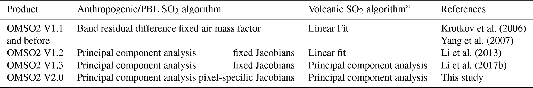
^∗ Volcanic SO₂ retrievals in all versions of OMSO2 use pixel-specific Jacobians.

While the OMI PBL SO₂ dataset produced with the PCA algorithm has significantly improved data quality as compared with the earlier version based on the BRD algorithm, the two algorithms share a common limitation: they both use a constant air mass factor (AMF) or SO₂ Jacobian spectrum for all pixels. The AMFs (or Jacobians) represent the sensitivity of OMI radiances to SO₂ total VCDs, and they depend on several factors including ozone amount and profile, SO₂ a priori profile shape, surface reflectivity, cloudiness, surface and cloud pressure, and solar and viewing zenith angles. The constant Jacobian spectrum used in the latest OMI PBL SO₂ dataset (OMSO2 V1.3) is precomputed with the VLIDORT radiative transfer (RT) code (Spurr, 2008), assuming cloud-free conditions with SO₂ predominantly in the lowest 1 km of the atmosphere. The spectrum does not take into account variations in geometry, O₃, clouds, or surface reflectivity (see Li et al., 2013 for details). This simplification enhances computation efficiency but also results in relatively large biases, particularly for pixels over cloudy scenes or background areas and pixels near the edges of the swath where absorption due to O₃ can substantially change SO₂ Jacobians.

Here, we describe the version 2 OMI SO₂ total vertical column density product (OMSO2 V2). As with the previous versions, OMSO2 V2 includes datasets for both volcanic and anthropogenic SO₂. As compared with OMSO2 V1.3, the volcanic SO₂ dataset in OMSO2 V2 is largely unchanged, while the anthropogenic SO₂ algorithm has seen some major updates and will be the focus of this paper. In particular, a set of new lookup tables and model-based a priori profiles are now used to estimate Jacobians for anthropogenic SO₂ retrievals for each individual pixel, thus better characterizing the sensitivity to SO₂ at different parts of the OMI sensor swath (e.g., nadir pixels vs. swath edges), over different regions (e.g., polluted vs. clean), and in different seasons (e.g., summer vs. winter). This helps to further improve the retrieval quality. The rest of the paper is organized as follows: in Sect. 2 we provide a description of the new OMI anthropogenic SO₂ algorithm. This is followed by data quality assessment in Sect. 3 and examples from the new anthropogenic SO₂ dataset in Sect. 4.

2 Algorithm description

2.1 Algorithm overview

The new anthropogenic SO₂ algorithm for OMSO2 V2 introduces several new components but retains the overall framework of the original PCA-based OMI PBL SO₂ algorithm that has been described in detail elsewhere (Li et al., 2013). Briefly, the algorithm employs a PCA technique to the measured radiance spectra from a number of satellite pixels to extract spectral features in the form of principal components (PCs). The PCs are ranked in a descending order according to their spectral variance content. In the absence of large SO₂ plumes, the leading PCs that contain the most variance (see Fig. 1 in Li et al. 2013 for an example) are typically associated with physical processes other than SO₂ absorption (e.g., ozone absorption, rotational Raman scattering) or some measurement features (e.g., wavelength shift, dark current). By fitting a set of n_ν PCs (ν_i) along with SO₂ Jacobians ($\frac{\partial N}{\partial {\mathrm{\Omega }}_{{\mathrm{SO}}_{\mathrm{2}}}})$ to the measured radiances, we obtain an estimate of the SO₂ VCD (Ω_SO2), at the same time minimizing the interferences from those processes represented by the PCs:

$$\begin{array}{}\text{(1)}& N\left(\mathit{\omega },{\mathrm{\Omega }}_{{\mathrm{SO}}_{\mathrm{2}}}\right)={\sum }_{i=\mathrm{1}}^{n_v}{\mathit{\omega }}_i{v}_i+{\mathrm{\Omega }}_{{\mathrm{SO}}_{\mathrm{2}}}{\displaystyle \frac{\partial N}{\partial {\mathrm{\Omega }}_{{\mathrm{SO}}_{\mathrm{2}}}}},\end{array}$$

where N is for the sun-normalized radiance spectrum for a satellite pixel in N value ($N\left(\mathit{\lambda }\right)=-\mathrm{100}\times {\log }_{\mathrm{10}}(I_{\mathrm{meas}}$ (λ)∕F(λ), I_meas and F are the measured radiance and solar irradiance at wavelength λ, respectively), and ω_i is the derived coefficient for the PC ν_i. For OMI retrievals, the algorithm processes one orbital swath at a time, with each swath comprising 60 rows (also referred to as cross-track positions) across the flight direction of the Aura spacecraft (cross-track) and each row containing ∼ 1600 pixels along the flight direction (along-track). For each swath, the algorithm also conducts PCA and spectral fit for each row separately, effectively treating them as different detectors.

The algorithm flowchart in Fig. 1 provides an overview of the new OMI anthropogenic SO₂ algorithm. It consists of three main components: (1) preprocessing and data filtering in order to select certain pixels within an OMI row for PCA analysis, (2) initial estimates of SO₂ vertical column densities (VCDs) made assuming a constant Jacobian spectrum, and (3) determination of pixel-specific Jacobians and final estimates of SO₂ VCDs. More detailed descriptions of these components are given below.

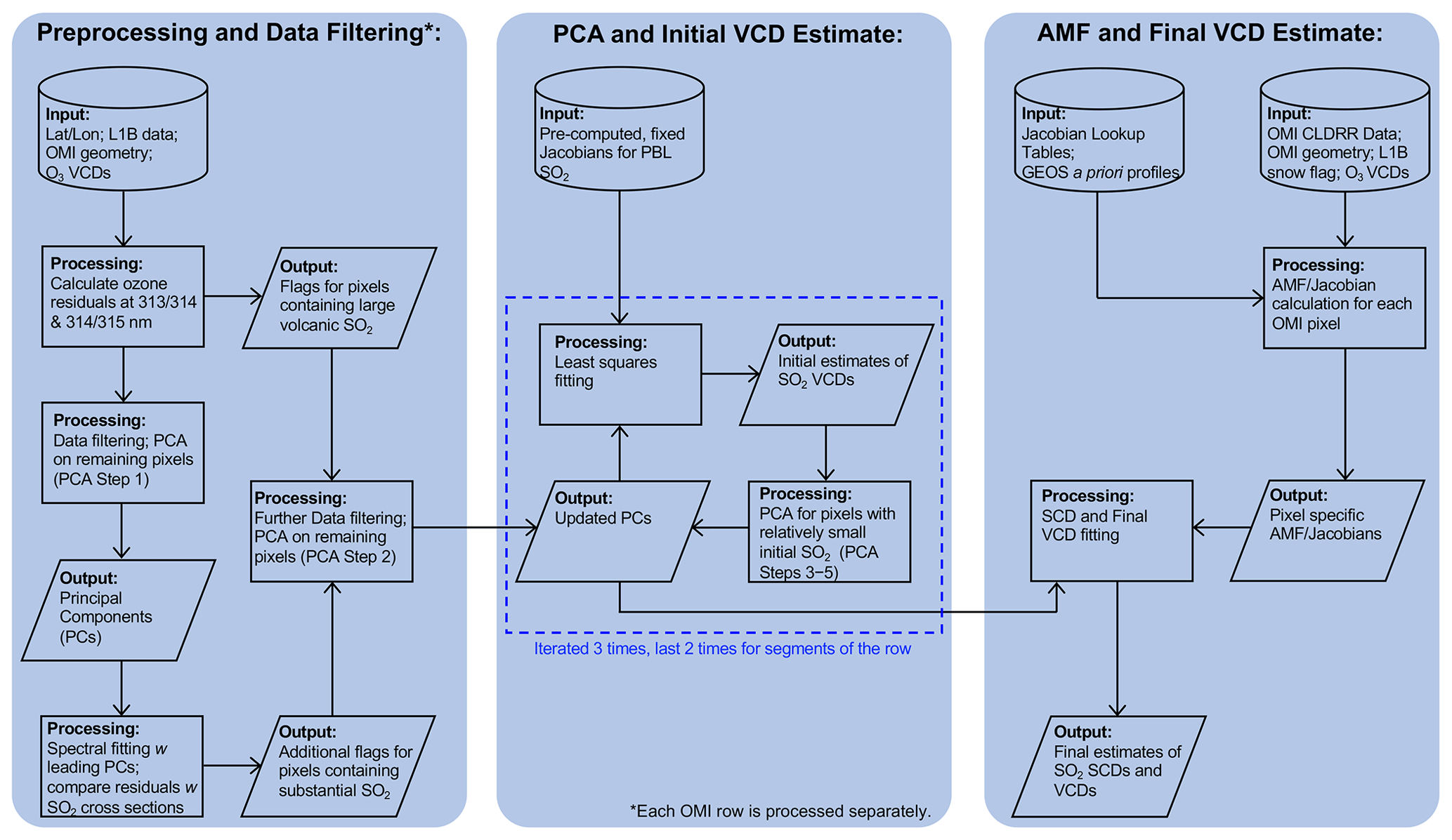
Figure 1 Flowchart of the PCA-based spectral fitting algorithm for the anthropogenic SO₂ dataset in the OMSO2 V2 product.

2.2 Preprocessing and data filtering

An important prerequisite for the spectral fit in Eq. (1) to work properly is that the PCs contain minimal spectral structures from SO₂ absorption. This condition is satisfied for the vast majority of atmospheric scenarios, given that background SO₂ loading is normally quite small (< 0.1 Dobson units, 1 DU = 2.69×10¹⁶ molecules cm⁻²) over most areas. On the other hand, the absorption of radiances by SO₂ can be substantial in the presence of large volcanic plumes or over heavily polluted areas, leading to apparent SO₂ structures in some of the leading PCs. The preprocessing and data-filtering component of the algorithm aims to flag those pixels with strong SO₂ signals and exclude them from the PCA analysis, thus minimizing their impacts on the spectral fit. Likewise, pixels having large solar zenith angles (SZAs > 75^∘) or affected by the OMI row anomaly (signal suppression at certain OMI rows; see Schenkeveld et al., 2017, for more information) are also filtered out using the dynamic row anomaly flag from the OMI L1B data. It should be pointed out that SO₂ VCD retrievals are conducted for all pixels with SZA < 75^∘ that are unaffected by the row anomaly, even if they are flagged for SO₂ and excluded from the PCA analysis.

In the first step of data preprocessing, pixels with relatively large volcanic signals are flagged based on ozone retrieval residuals from two wavelength pairs (313/314 and 314/315 nm). We first estimate OMI radiances at these wavelengths using the total column O₃ from the OMTO3 product (Bhartia, 2005) in conjunction with the simple Lambertian equivalent reflectivity (SLER) derived at the surface (Ahmad et al., 2004), assuming no SO₂. The residuals are the differences between the measured and estimated logarithmic radiances. When there is indeed little SO₂ in the atmosphere, the residuals are similar for the wavelength pairs (e.g., 313 and 314 nm). For volcanic eruptions, however, the residuals at 313 nm become much greater due to stronger SO₂ absorption that is unaccounted for in O₃ retrievals. A large difference in O₃ residuals between 313 and 314 nm or between 314 and 315 nm for a given pixel thus signals relatively large abundance of SO₂, and that pixel is flagged. Side-by-side comparisons between the flagged pixels and OMI volcanic SO₂ retrievals (Li et al., 2017b) indicate that the flagging scheme is effective at identifying pixels with ∼ 5 DU or more of SO₂ (assuming plume centered at ∼ 18 km).

The second step of the preprocessing attempts to further screen for SO₂. After rejecting pixels with large SZAs or flagged for volcanic SO₂, the measured radiance spectra between 310.5 and 340 nm from the remaining (typically ∼ 1200–1300) pixels in the row are subject to a PCA analysis. As large volcanic SO₂ signals have already been screened out, the first five derived PCs are usually free from SO₂ spectral structures. We fit those PCs to the measured radiances and calculate fitting residuals for each pixel. Without SO₂ structures in the PCs or the SO₂ Jacobian term on the right-hand side (RHS) of Eq. (1), the fitting residuals for a pixel having sizable SO₂ (e.g., those over heavily polluted areas) are expected to be correlated with the SO₂ cross sections. We flag pixels that have a relatively large absolute cross product between the fitting residuals and a normalized spectrum of SO₂ cross sections.

In the final step of the preprocessing, a second PCA analysis is conducted for the radiance spectra within 310.5–340 nm from a given OMI row, this time excluding all pixels that have been flagged for SO₂. The resulted PCs are used as input to the second component of the algorithm for initial estimates of SO₂ VCDs.

2.3 Initial estimates of SO₂ VCDs

To make initial estimates of SO₂ VCDs (Ω_{SO2_ini}), we carry out a spectral fit following Eq. (1) using the first six PCs from the final preprocessing step (see Sect. 2.2) along with a fixed SO₂ Jacobian spectrum identical to that for the PBL SO₂ retrievals in OMSO2 V1.3. Pixels that are not flagged for SO₂ in the preprocessing and have relatively small initial SO₂ VCDs, with −2σ < Ω_{SO2_ini} < 1.5σ (where σ is the standard deviation of Ω_{SO2_ini}), are selected for a new round of PCA analysis. The updated PCs are then used in another spectral fit to produce updated VCD estimates (Fig. 1). Note that the threshold for pixel selection was set at ±1.5σ in our previous PBL SO₂ algorithm (Li et al., 2013). Now the lower limit has been relaxed to reduce the minor negative biases over some areas in the previous product. Additionally, the threshold is further relaxed by 50 %, to −3σ < Ω_{SO2_ini} < 2.25σ for pixels with SZA > 60^∘, considering that the VCDs at larger solar zenith angles tend to be noisier due to lower signal-to-noise ratio in the radiance data.

This process of spectral fit, pixel selection, updated PCA, and updated spectral fit as described above is repeated three times. For the last two iterations, the OMI row is divided into three subsectors based on the SZAs: a tropical subsector with small solar zenith angles (SZA < SZA${}_{\min }+\mathrm{0.4}\times$ (75^∘ – SZA_min), where SZA_min is the minimal SZA of the row) and two extratropical ones south and north of it. As discussed in Li et al. (2013), PCs derived from these subsectors more closely represent local observation conditions and reduce retrieval noise and biases. For these two iterations, we also use up to n_ν=30 PCs in the spectral fit. The exact value of n_ν is determined by checking the correlation between the PCs and the SO₂ cross sections. If for example the ith PC has significant SO₂ spectral structures, only n_ν=i–1 PCs are used in the spectral fit (see Li et al., 2013, for more discussion on the number of PCs included in the fit). With effective SO₂ screening steps in data preprocessing (Sect. 2.2), n_ν=30 PCs are used in the fit most of the time. Also as pixels affected by row anomaly are excluded from retrievals during the data-filtering step (see Sect. 2.2), the OMI row anomaly has a minimal effect on n_ν. After these three iterations, the finalized PCs are transferred to the third component of the algorithm.

2.4 Determination of SO₂ Jacobians and final estimates of SO₂ VCDs

In the third and final component of the algorithm, we use the finalized PCs (Sect. 2.3) and the SO₂ cross sections (in place of Jacobians in Eq. 1) to estimate SO₂ slant column densities (SCDs). In addition, we also use pixel-specific Jacobian spectra for the final SO₂ VCDs. To this end, we employ a table lookup approach and model-based a priori profiles to estimate SO₂ Jacobians for individual OMI pixels (Sect. 2.4.1 and 2.4.2). Special consideration is required for pixels covered by snow or ice (Sect. 2.4.3), as well as those over areas affected by the South Atlantic Anomaly (SAA, Sect. 2.4.4)

2.4.1 Jacobian lookup tables

The total column SO₂ Jacobians ($\frac{\partial \ln \left(I\right)}{\partial {\mathrm{\Omega }}_{\mathrm{SO}\mathrm{2}}})$ and AMFs ($-\frac{\partial \ln \left(I\right)}{\partial {\mathit{\tau }}_{\mathrm{SO}\mathrm{2}}})$ represent the sensitivity of the natural logarithm of top of atmosphere (TOA), sun-normalized radiances ($I=I_{\mathrm{meas}}/F$, the ratio between the measured radiances, I_meas, and solar irradiances, F) to perturbations in SO₂ VCD (Ω_SO2) and SO₂ optical thickness (τ_SO2) in the entire atmospheric column, respectively. The two derivatives are linked through the absorption cross sections of SO₂. They can be calculated from the vertically resolved layer Jacobians (or box AMFs) and a priori profile shape of SO₂, for example

$$\begin{array}{}\text{(2)}& {\displaystyle \frac{\partial \ln \left(I\right)}{\partial {\mathrm{\Omega }}_{\mathrm{SO}\mathrm{2}}}}={\int }_{\mathrm{0}}^{\mathrm{TOA}}m\left(z\right)n_{\mathrm{SO}\mathrm{2}}\left(z\right)\mathrm{d}z,\end{array}$$

where n_SO2(z) is the normalized a priori profile or shape factor that represents the fraction of SO₂ molecules in layer z to the overall number of SO₂ molecules in the entire column. The layer Jacobians (sometimes also referred to as scattering weights), m(z), are defined as the sensitivity of ln(I) to changes in Ω_SO2(z), the partial column SO₂ density within layer z:

$$\begin{array}{}\text{(3)}& m\left(z\right)={\displaystyle \frac{\partial \ln \left(I\right)}{\partial {\mathrm{\Omega }}_{\mathrm{SO}\mathrm{2}}\left(z\right)}}.\end{array}$$

Sun-normalized TOA radiances I and layer Jacobians m(z) at a wavelength λ depend on several factors including O₃ (both the total amount and vertical distribution), observation geometry, and the pressure and reflectivity of the underlying clouds or surfaces. Following the same parameterization approach as in Li et al. (2017b), I in a Rayleigh atmosphere can be calculated with the following equation:

$$\begin{array}{}\text{(4)}& \begin{array}{rl}I& =I_{\mathrm{0}}\left({\mathit{\theta }}_{\mathrm{0}},\mathit{\theta }\right)+I_{\mathrm{1}}\left({\mathit{\theta }}_{\mathrm{0}},\mathit{\theta }\right)\cos \mathit{\varphi }+I_{\mathrm{2}}\left({\mathit{\theta }}_{\mathrm{0}},\mathit{\theta }\right)\cos \mathrm{2}\mathit{\varphi }\\ & +{\displaystyle \frac{{\mathrm{RI}}_{\mathrm{r}}\left({\mathit{\theta }}_{\mathrm{0}},\mathit{\theta }\right)}{\left(\mathrm{1}-{\mathrm{RS}}_{\mathrm{b}}\right)}},\end{array}\end{array}$$

where θ₀, θ, and ϕ stand for SZA, viewing zenith angle (VZA), and relative azimuth angle (RAA), respectively. I₀, I₁, and I₂ are Fourier expansion coefficients in ϕ; together these terms represent the atmospheric component of I. The fourth term on the RHS of Eq. (4) represents the surface component of I, in which RI_r is the TOA radiance reflected once by the underlying surface (that has a Lambertian reflectivity of R) and transmitted through the atmosphere, S_b is the fraction of the surface-reflected radiance that is scattered back to the surface, and (1–RS_b) accounts for the multiple reflections between the surface and the atmosphere. The layer Jacobians can then be parameterized differentiating Eq. (4):

$$\begin{array}{}\text{(5)}& \begin{array}{rl}m\left(z\right)& =\left[{\displaystyle \frac{\partial I_{\mathrm{0}}\left({\mathit{\theta }}_{\mathrm{0}},\mathit{\theta }\right)}{\partial {\mathrm{\Omega }}_{\mathrm{SO}\mathrm{2}}\left(z\right)}}+{\displaystyle \frac{\partial I_{\mathrm{1}}\left({\mathit{\theta }}_{\mathrm{0}},\mathit{\theta }\right)}{\partial {\mathrm{\Omega }}_{\mathrm{SO}\mathrm{2}}\left(z\right)}}\cos \mathit{\varphi }\right.\\ & +{\displaystyle \frac{\partial I_{\mathrm{2}}\left({\mathit{\theta }}_{\mathrm{0}},\mathit{\theta }\right)}{\partial {\mathrm{\Omega }}_{\mathrm{SO}\mathrm{2}}\left(z\right)}}\cos \mathrm{2}\mathit{\varphi }+{\displaystyle \frac{R}{\left(\mathrm{1}-{\mathrm{RS}}_{\mathrm{b}}\right)}}{\displaystyle \frac{\partial I_{\mathrm{r}}\left({\mathit{\theta }}_{\mathrm{0}},\mathit{\theta }\right)}{\partial {\mathrm{\Omega }}_{\mathrm{SO}\mathrm{2}}\left(z\right)}}\\ & \left.+{\displaystyle \frac{R^{\mathrm{2}}{I}_{\mathrm{r}}\left({\mathit{\theta }}_{\mathrm{0}},\mathit{\theta }\right)}{{\left(\mathrm{1}-{\mathrm{RS}}_{\mathrm{b}}\right)}^{\mathrm{2}}}}{\displaystyle \frac{\partial S_{\mathrm{b}}}{\partial {\mathrm{\Omega }}_{\mathrm{SO}\mathrm{2}}\left(z\right)}}\right]\cdot I^{-\mathrm{1}}.\end{array}\end{array}$$

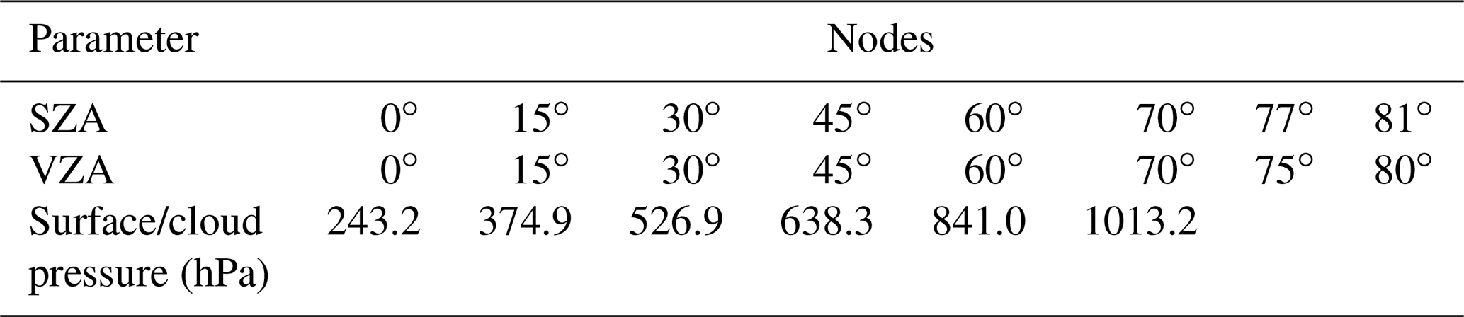
With Eqs. (4) and (5), we can determine the layer Jacobians for any given ϕ and R from multidimensional lookup tables that contain I₀, I₁, I₂, I_r, and S_b and their derivatives with respect to Ω_SO2(z) for different SZAs, VZAs, underlying surface/cloud pressures, and O₃ amounts and profiles. To account for the effects of O₃ on layer Jacobians, we use a climatology of ozone profiles that depends on the total ozone amount developed by Labow et al. (2015) from ozone sonde and Microwave Limb Sounder (MLS) measurements. The profile Jacobian elements in Eq. (5) may be calculated conveniently using the VLIDORT radiative transfer model, which has the ability to generate any sets of analytically calculated Jacobians in a polarized multilayer atmosphere. For each of the 46 ozone climatology profiles, we ran the VLIDORT to build a Jacobian lookup table (LUT) with dimensions of 6 × 8 × 8 × 72 × 801. The first three dimensions (6 × 8 × 8) correspond to the different nodes in the lookup table for the underlying surface/cloud pressures, SZAs, and VZAs (see Table 2 for details). The last two dimensions are necessary for storing vertically (72 layers, 0.01–1013.25 hPa) and spectrally (305–345 nm at 0.05 nm resolution) resolved parameters for Jacobians.

Table 2 Nodes of the solar zenith angle (SZA), viewing zenith angle (VZA), and surface/cloud pressure, as used in the precomputed SO₂ Jacobians lookup tables.

The effects of clouds on SO₂ Jacobians are accounted for with the independent pixel approximation (IPA) approach that is commonly employed in UV/VIS trace gas retrievals (e.g., Ahmad et al., 2004; Koelemeijer et al., 2001; Martin et al., 2002; Seftor et al., 1994). For each OMI pixel, we use multidimensional interpolation to estimate layer Jacobians for both cloudy and cloud-free parts of the pixel. For the cloudy part, the optical centroid cloud pressure (OCP) from the OMI Raman scattering cloud product (OMCLDRR, Joiner and Vasilkov, 2006), retrieved at wavelengths near the SO₂ fitting window, is used and R is taken to be 0.8. For the cloud-free part, the surface reflectivity and surface pressure assumed in OMCLDRR retrievals are used. The cloudy (m_cld(z)) and cloud-free (m_clr(z)) layer Jacobians at layer z are weighted with the cloud radiance fraction (CRF) in the SO₂ fitting window:

$$\begin{array}{}\text{(6)}& m\left(z\right)=m_{\mathrm{cld}}\left(z\right)\mathrm{CRF}+m_{\mathrm{clr}}\left(z\right)\left(\mathrm{1}-\mathrm{CRF}\right),\end{array}$$

$$\begin{array}{}\text{(7)}& \mathrm{CRF}=f_{\mathrm{c}}{\displaystyle \frac{I_{\mathrm{cld}}}{I_{\mathrm{meas}}}},\end{array}$$

where I_meas and I_cld are measured TOA radiances and estimated cloudy radiances, respectively, and f_c is the effective cloud fraction retrieved by the OMCLDRR algorithm. Following Eq. (2), the interpolated layer Jacobian profile is combined with the a priori profile shape factor selected based on the latitude, longitude, and time (month of the year) of the OMI measurement (see Sect. 2.4.2) to produce SO₂ column Jacobians between 305 and 340 nm at 0.05 nm resolution. The high-resolution Jacobians are then convolved using the OMI slit function.

2.4.2 GEOS-5 a priori profiles

For a priori profile shape factors (n_SO2(z)), we use GEOS-5 (Goddard Earth Observing System, Version 5) global model simulations (72 vertical layers, 0.5^∘ latitude by 0.667^∘ longitude horizonal resolution) for the time period 2004–2014. The output from GEOS-5 is sampled at the OMI overpass time and normalized against the model-simulated total SO₂ VCD within each grid cell to produce monthly shape factor profiles. For each month of the year, these shape factor profiles are then averaged over the entire simulation period to generate monthly climatology profiles for use as a priori in our SO₂ retrievals.

2.4.3 Retrievals for pixels covered by snow or ice

From Eq. (5), one would expect that highly reflective snow/ice-covered surfaces could enhance the sensitivity of OMI to SO₂ particularly at lower altitudes. Retrievals over these areas in the previous OMI PBL SO₂ dataset (OMSO2 V1.3) are however biased high, owing to the use of a constant Jacobian spectrum. Here we use OMCLDRR product and snow/ice flag in the OMI L1B data to identify pixels that are cloud-free and covered by snow/ice, following an approach proposed by Vasilkov et al. (2010). For OMI pixels flagged for snow/ice in the L1B data (OML1BRGU), we compare the terrain pressure with the effective scene pressure retrieved by the OMCLDRR algorithm (Joiner and Vasilkov, 2006). If the difference between the two is within 50 hPa, the pixel is likely cloud-free. We then assume a cloud fraction of zero and use the simple Lambertian equivalent reflectivity (SLER) derived for that pixel in Jacobian calculations. On the other hand, if the difference is greater than 100 hPa, the pixel is likely cloudy, and the cloud fraction is set to one in Jacobian calculations. For pixels having scene and terrain pressure differences between 50 and 100 hPa, unambiguous cloud detection is not possible. While we still assume cloud-free conditions in the Jacobian calculations for such pixels, they are flagged and should be excluded from data analysis due to greater uncertainty.

2.4.4 Retrieval noise suppression for areas affected by the South Atlantic Anomaly

Polar-orbiting satellite sensors like OMI are often subject to greater fluxes of high-energy particles when flying over areas affected by the South Atlantic Anomaly (SAA), leading to larger noise in trace gas retrievals. Following Richter et al. (2011), we have implemented a two-step spectral fit to suppress SO₂ retrieval noise over the SAA region. The scheme examines the spectral fitting residual at each wavelength between 310.5 and 340 nm for all OMI pixels within the SAA region (defined here as the domain 0–45^∘ S, 100^∘ W–5^∘ E). If a pixel has wavelengths with relatively large fitting residuals (beyond ±0.2 N value), these wavelengths are excluded in a second step spectral fit that produces the final SO₂ VCD for the pixel. As shown in the following sections, this two-step scheme effectively reduces retrieval noise over the SAA region.

3 Quality assessment

Uncertainties in the retrieved SO₂ VCDs arise from both the spectral fit and the Jacobian calculation parts of the algorithm that are largely independent from each other. Uncertainties in the former can originate from measurement errors as well as the basis functions (i.e., the PCs) and can be represented as uncertainties in SO₂ SCDs. On the other hand, uncertainties in the SO₂ Jacobians are primarily due to the various assumptions inherent in the radiative transfer model and also to uncertainties in input parameters used in the RT calculations. In this section, we assess the uncertainties (Sect. 3.1) and long-term stability (Sect. 3.2) in SCDs, and we also discuss various factors that contribute to the uncertainties in SO₂ Jacobians (Sect. 3.3).

3.1 Uncertainties in slant column densities (SCDs)

Two different methods have been used to estimate uncertainties in SO₂ SCDs: the first based on the fitting residuals with an approach similar to that for DOAS uncertainty estimates and the other based on a statistical analysis of SO₂ SCDs over the remote Pacific.

3.1.1 SCD uncertainties estimated from fitting residuals

We can express the basis functions on the RHS of Eq. (1) in terms of a matrix A that has dimensions of K×M. The number of columns in A, $M=n_{\mathit{\nu }}+\mathrm{1}$, represents the n_ν PCs plus the SO₂ cross-section spectrum included in the least squares fit, whereas the row dimension K is the number of OMI wavelengths at which the PCs and SO₂ cross sections are specified. Following a common approach for estimating uncertainty in DOAS spectral fitting (e.g., Zara et al., 2018), the uncertainty (ε_j) in the jth fitted parameter is the square root of the jth diagonal element of the covariance matrix:

$$\begin{array}{}\text{(8)}& {\mathit{\epsilon }}_j=\sqrt{{\mathit{\chi }}^{\mathrm{2}}{\left(A^{T}A\right)}_{jj}^{-\mathrm{1}}},\end{array}$$

where χ² can be calculated from the fitting residuals (r(λ_k), the difference between the measured and fitted N values) at all wavelengths in the fitting window and the degree of freedom (K−M):

$$\begin{array}{}\text{(9)}& {\mathit{\chi }}^{\mathrm{2}}={\displaystyle \frac{\mathrm{1}}{K-M}}\sum _{k=\mathrm{1}}^{k=K}{r}^{\mathrm{2}}\left({\mathit{\lambda }}_k\right).\end{array}$$

The estimated SCD uncertainties for four selected OMI swaths over the remote Pacific in different seasons in 2007 are given in Fig. 2i–l, along with the SCDs (Fig. 2a–d) and scene reflectivity at 354 nm (Fig. 2e–h). As can be seen from the plots, the SCD uncertainties for most pixels are within the range of 0.05–0.25 DU and demonstrate substantial spatial variability. To the first order, there is an apparent connection between the estimated uncertainties and the reflectivity. Pixels over bright surfaces covered by clouds (e.g., east of New Zealand in orbit 13160) or snow/ice (e.g., over the Antarctica) often have smaller uncertainties. This is probably due to enhanced signal-to-noise ratio in OMI-measured radiances over highly reflective scenes, suggesting that the measurement noise is probably a driving factor for SCD uncertainties. The estimated SCD uncertainties are also generally greater at higher latitudes, again probably reflecting strong light extinction and reduced signal-to-noise ratio at larger solar zenith angles and larger O₃ amounts. There is also a gradient in SCD uncertainties, for example, just south of Hawaii in orbit 13160. Recall that pixels from each row are grouped into three subsectors for the final PCA (see Sect. 2.4), based on their solar zenith angles. And the gradient is likely caused by the changes in basis functions (i.e., the PCs) over the transition zones between the tropical and the extratropical subsectors. Additionally, the SCD uncertainties also show some cross-track dependence particularly at lower latitudes, being mostly smaller on the eastern side of the swath than on the western side. The reason for this cross-track difference is not yet fully understood, but it could be due to stronger reflection of sky light on the eastern side of the swath over ocean (Vasilkov et al., 2017). Similar cross-track dependence has also been found over land and could be due to generally stronger scattering in the backscattering direction (on the eastern side) than in the forward scattering direction (on the western side), as demonstrated by Qin et al. (2019).

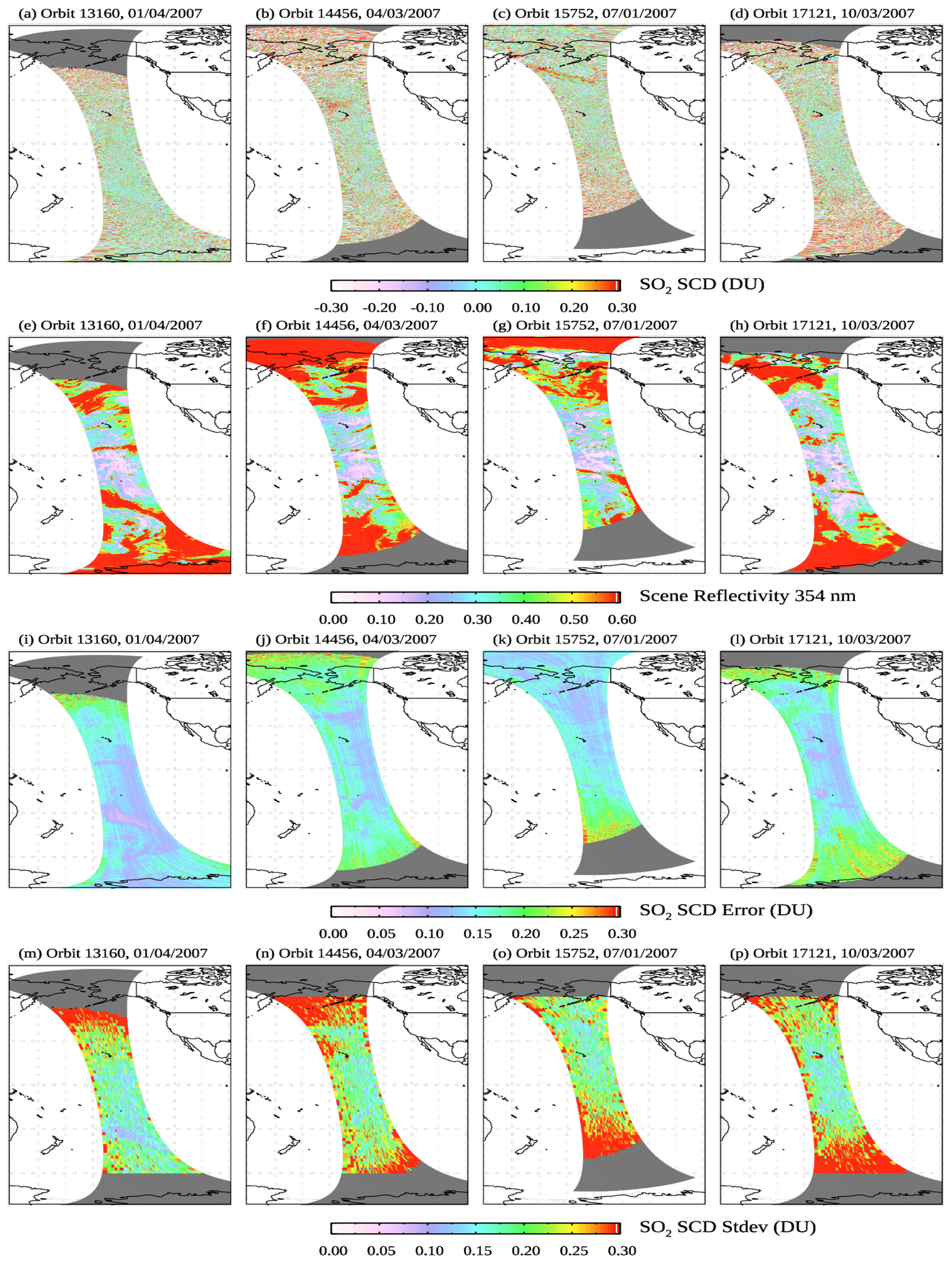
Figure 2 (a–d) The SO₂ slant column densities for four OMI swaths over the remote Pacific on (a) 4 January, (b) 3 April, (c) 1 July, and (d) 3 October 2007. (e–h) The reflectivity at 354 nm for the same swaths. (i–l) Estimated uncertainties in SO₂ slant column densities (ε_SCD) for the same swaths. Cloudy or snow/ice-covered areas have greater reflectivity and generally smaller errors in SO₂ SCDs. No retrievals were attempted for pixels with SZA > 75^∘ that are grey-shaded. (m–p) The standard deviation of SO₂ SCDs (σ_SCD) within 2^∘ latitude segments of individual OMI rows for the same swaths. The spatial coverage for panels (m–p) is limited to 60^∘ S to 60^∘ N as changes in observation conditions tend to be larger at higher latitudes. In addition, pixels with SCD > 2 DU or SZA > 75^∘ and segments with < 10 valid pixels are excluded from the statistical analysis.

As expected, the retrieved SCDs are quite small over the remote Pacific covered by these swaths (Fig. 2a–d). As a result, the relative uncertainties (calculated as the ratio between the estimated uncertainties and the retrieved SCDs) are fairly large (see Fig. S1 in the Supplement). About half of the pixels have relative uncertainties within ±100 %, and ∼80 % have relative uncertainties within ±275 %. In contrast, pixels that have substantial real SO₂ signals (e.g., downwind of the Kīlauea volcano in Hawaii) have relative uncertainties of ∼ 20 %–50 %.

3.1.2 SCD uncertainties estimated from statistical analysis

Another common way to assess SCD uncertainties is to calculate the standard deviation of SCDs over background areas that have small natural variability in SO₂ such as the equatorial Pacific (e.g., Li et al., 2013). In Fig. 2m–p, we map the standard deviation of SO₂ SCDs within 2^∘ latitude segments of each row for the same OMI swaths as in Fig. 2i–l. Calculations are limited to 60^∘ S–60^∘ N, as SZAs and ozone amounts tend to be more variable at higher latitudes. Also, pixels with large SCDs (> 2 DU) are excluded. As compared with the SCD uncertainties estimated from the fitting residuals (hereafter referred to as ε_SCD), the standard deviation of SCDs (hereafter referred to as σ_SCD) is considerably greater especially at higher latitudes. This is to be expected, given that σ_SCD includes not only just noise from the spectral fit, but the natural variability in SCDs. For instance, σ_SCD is enhanced downwind of Hawaii (Fig. 2p), likely reflecting larger variability caused by the SO₂ plume from the Kīlauea volcano (Fig. 2d). As for the spatial pattern, there are similarities between σ_SCD and ε_SCD, with both being generally smaller at low latitudes and over clouds. As with ε_SCD, σ_SCD also appears to be smaller on the eastern side of the swath.

A more detailed comparison between ε_SCD and σ_SCD for selected OMI rows can be found in Fig. 3. ε_SCD is ∼ 0.15 DU over the equatorial Pacific (20^∘ S–20^∘ N) and, with few exceptions, is mostly < 0.2 DU at all latitudes. σ_SCD shows much larger variability, ranging from ∼ 0.2 DU near the Equator to over 0.5 DU at around 60^∘ S and 60^∘ N in some cases. The difference between ε_SCD and σ_SCD is generally less than 0.1 DU at low latitudes but can exceed 0.2 DU at high latitudes. If we consider ε_SCD as a lower bound for SCD uncertainties and σ_SCD as an upper bound, we arrive at the conclusion that the SCD uncertainties from the new algorithm are ∼ 0.15–0.3 DU between ∼ 40^∘ S and ∼ 40^∘ N and ∼ 0.2–0.5 DU at higher latitudes. For a moderately polluted area in the middle latitudes (e.g., ∼ 30–40^∘ N) with an SCD of ∼ 0.3 DU, this translates into a relative uncertainty of ∼ 50 %–100 %.

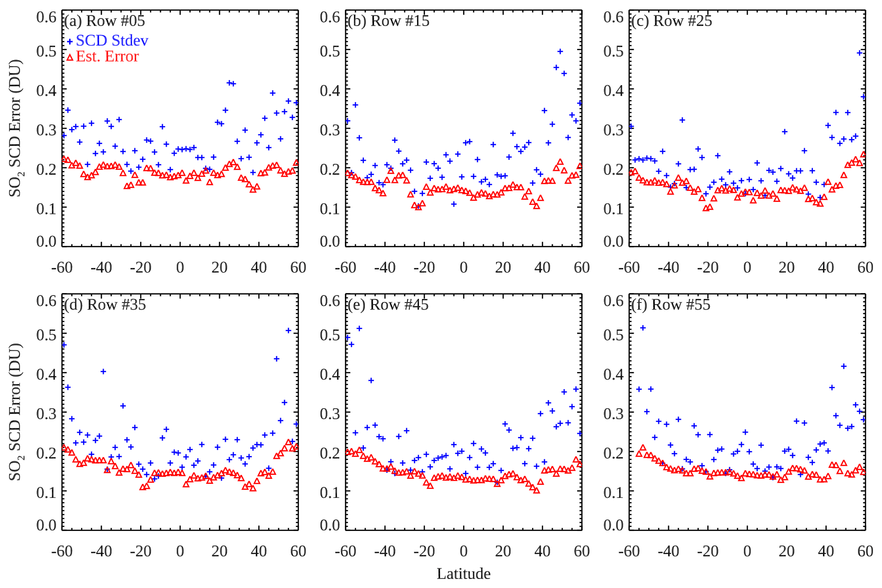
Figure 3 Mean SO₂ SCD uncertainties estimated from fitting residuals (ε_SCD, red triangles) and SCD standard deviation (σ_SCD, blue plus signs) for 2^∘ latitude segments between 60^∘ S and 60^∘ N from selected OMI rows from orbit 14456 on 3 April 2007.

3.2 Long-term changes in SCDs over remote background areas

Drift in retrievals over background areas may introduce artificial trends or mask actual trends over polluted regions, and the long-term stability in the OMI anthropogenic SO₂ dataset is of great importance for detecting regional changes. Here we examine temporal changes in SCDs from the new algorithm over the equatorial east Pacific (20^∘ S–20^∘ N, 130–150^∘ W) throughout the OMI record from October 2004 to December 2019. To ensure consistency in sampling, we only use data from rows 6–24 (1-based) that are considered to be minimally affected by the OMI row anomaly. Following McLinden et al. (2016), we also try to minimize the impact of volcanic eruptions. This is achieved by excluding days when the 99th percentile of SO₂ SCDs over the east Pacific (80^∘ S–80^∘ N, 130–150^∘ W) exceeds 0.8 DU. The daily median and mean of SO₂ SCDs for the equatorial east Pacific are shown in Fig. 4a and b, respectively. A linear regression analysis indicates that both median and mean SCDs have statistically significant (the linear correlation coefficient, r=0.18, and p<0.05 from two-tailed t test) but very small changes over time, at $\mathrm{2.0}\times {\mathrm{10}}^{-\mathrm{4}}$ and $\mathrm{2.3}\times {\mathrm{10}}^{-\mathrm{4}}$ DU per year, respectively. In other words, over the entire ∼ 15-year OMI record to date, the daily mean of background SO₂ SCDs has only increased slightly by ∼ 0.0035 DU (∼ 0.003 DU for median). This long-term stability in the SO₂ record is an indicator of the stable performance of the OMI instrument itself (Schenkeveld et al., 2017), and it also confirms the ability of the PCA-based retrieval method to account for some of the drifts in measurements.

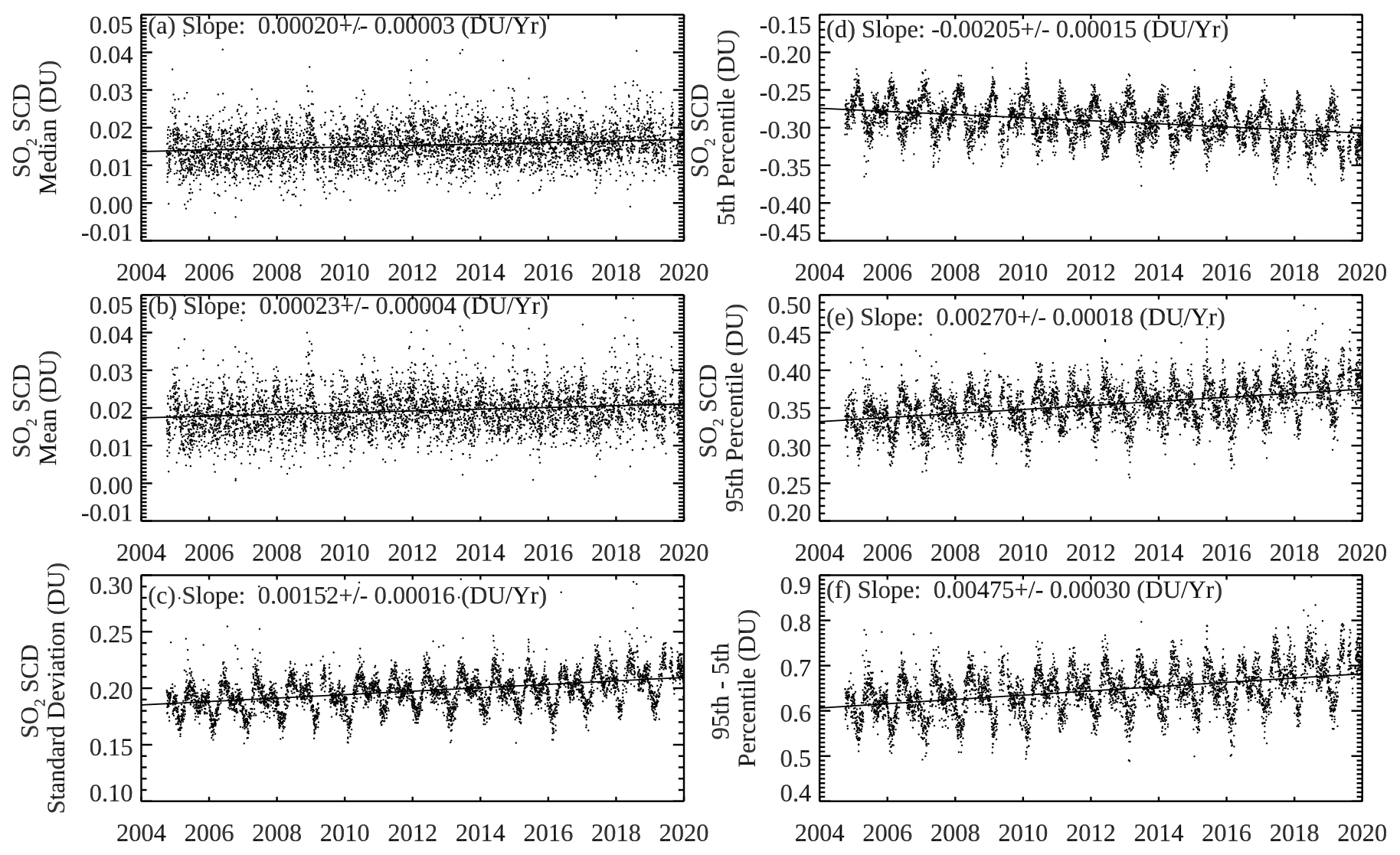
Figure 4 Daily (a) median, (b) mean, (c) standard deviation, (d) 5th percentile, (e) 95th percentile, and (f) the difference between 5th and 95th percentiles of OMI SO₂ SCDs over the equatorial east Pacific (20^∘ S–20^∘ N, 130–150^∘ W) during the period of 2004–2019 indicate stable long-term performance of the PCA-based anthropogenic SO₂ algorithm. Estimated linear trends and their 95 % confidence intervals are given for each time series. Only rows deemed to be minimally affected by the row anomaly are included in the statistical analysis. Days with possible influence of large volcanic SO₂ eruptions have also been excluded.

On the other hand, the standard deviation of SO₂ SCDs (Fig. 4c) over the equatorial east Pacific shows more notable changes, growing from ∼ 0.19 DU in 2005 to ∼ 0.21 DU in 2019 at a rate of $\sim \mathrm{1.5}\times {\mathrm{10}}^{-\mathrm{3}}$ DU per year. This represents an approximately 10 % increase in SCD uncertainties in ∼ 15 years. The well below 1 % per year rise in retrieval noise can be attributed to instrument degradation over time (Schenkeveld et al., 2017). A recent study (Zara et al., 2018) reports a faster growth rate in the uncertainties for OMI NO₂ retrievals (1 %–2 % per year) and a more comparable rate for HCHO retrievals (< 1 % per year). Note that NO₂ retrievals rely on measurements at visible wavelengths from a different detector (VIS) of the OMI instrument than SO₂ and HCHO retrievals (UV-2).

An examination of the daily 5th and 95th percentiles of the SCDs (Fig. 4d and e) over the same area reveals larger changes in opposite directions, at $-\mathrm{2.0}\times {\mathrm{10}}^{-\mathrm{3}}$ and $\mathrm{2.7}\times {\mathrm{10}}^{-\mathrm{3}}$ DU per year, respectively. As a result, the spread or the difference (Fig. 4f) between these two time series has increased by a total of almost 0.1 DU over the 15-year period. These changes in the percentiles suggest that the growth in the standard deviation is likely driven by more outliers in the retrieved SCDs. Indeed, the distribution of SO₂ SCDs over the equatorial east Pacific has grown broader since 2005 (see Fig. S2 for plots of probability density function for different years). For 2005, 43.2 % (98.5 %) of the OMI pixels over the area have SCDs between −0.1 and 0.1 DU (−0.5 to 0.5 DU). The percentage has decreased to 41.3 % (98.1 %) by 2012 and further to 39.6 % (97.4 %) by 2019. Overall, the increase in the noise in the SCD retrievals is quite modest, pointing to good long-term stability of the new OMI anthropogenic SO₂ dataset.

3.3 Discussion on uncertainties in SO₂ Jacobians

In addition to the spectral fit, uncertainties in the SO₂ VCDs also depend on the Jacobian calculations. We have conducted several sensitivity tests using the VLIDORT RT code to investigate potential sources of uncertainties in Jacobians/AMFs. Note that these tests are not meant to be inclusive; rather, the aim is to shed some light on the relevance of different aspects in the error budget. Detailed results of these tests can be found in the Supplement (Figs. S3–S9). Here we summarize the potential error sources.

1. Uncertainties in forward radiative transfer model assumptions (such as SO₂ cross sections) and the table lookup interpolation scheme. Laboratory-measured cross sections usually have uncertainties < 10 %, and RT codes have uncertainties of about 5 % (Theys et al., 2017). Also, a fixed temperature profile was used in RT calculations in this study. In extreme cases where the seasonal temperature change can reach ∼ 50 ^∘C, this can cause up to ∼ 5 %–10 % error in SO₂ Jacobians (Fig. S3) due to the temperature dependence of the SO₂ cross sections that is unaccounted for. As for LUT interpolation, our tests indicate that the associated uncertainties should be generally within 5 %–10 % at altitudes relevant to anthropogenic SO₂ retrievals (Fig. S4).

2. Uncertainties in a priori profiles. Comparisons of monthly a priori profiles (Sect. 2.4.2) with available aircraft measurements (e.g., Dickerson et al., 2007) suggest that the climatology lacks the day-to-day variations associated with synoptic weather systems, and that may lead to ∼ 15 %–40 % of error for individual pixels over polluted regions such as northeastern China (Fig. S5). Model-simulated daily a priori profiles may better capture short-term changes in SO₂ vertical distribution but are currently not yet implemented in our retrievals.

3. Uncertainties in surface reflectivity, cloud fraction, and cloud pressure. Assuming a surface reflectivity of ∼ 0.05, a typical uncertainty of 0.01 causes ∼ 7% uncertainty in SO₂ Jacobians under cloud-free conditions (Fig. S6). Depending on the vertical distribution of SO₂ and cloud height, clouds can either enhance (albedo effect) or reduce (shielding effect) OMI sensitivity. For polluted areas where SO₂ is predominantly in the lower troposphere, an uncertainty of ∼ 0.05–0.1 in cloud fraction leads to an uncertainty of ∼ 5 %–10 % in Jacobians (Fig. S7), while an uncertainty of ∼ 50–100 hPa in cloud pressure translates into ∼ 25 %–40 % uncertainty in Jacobians (Fig. S8).

4. Lack of explicit consideration for aerosol effects on SO₂ Jacobians. In the IPA approach (Sect. 2.4.1), the contribution of aerosols to TOA radiances is treated as if they arose from clouds. As a result, the aerosol scattering effects are implicitly accounted for by including aerosols as part of the effective cloud fraction. For nonabsorbing or weakly absorbing aerosols (Fig. S9a and b), such implicit treatment may cause ∼ 10 %–30 % uncertainties in SO₂ Jacobians, but the sign (shielding vs. albedo effects) and the size of the errors are determined by the vertical distributions of aerosols and SO₂, as well as the cloud/scene pressures from the cloud algorithm. For UV absorbing aerosols such as dust and smoke (Mok et al., 2016), the uncertainties can amount to ∼ 50 % (Fig. S9c).

The estimated uncertainties for the above aspects are mostly comparable with the error analysis conducted by Theys et al. (2017) for the Copernicus Sentinel-5 precursor (TROPOMI) SO₂ algorithm. Both studies point to the importance of SO₂ a priori profiles, cloud pressure, and the implicit treatment of aerosol effects, with the latter two associated with the IPA approach. If we assume that all these uncertainty terms are independent, the overall uncertainties of column Jacobians/AMFs are estimated to be ∼ 30 %–80 % for individual pixels. For a polluted area where the uncertainties in SCDs are ∼ 50 %–100 %, the uncertainties in the retrieved SO₂ VCDs would be ∼ 60 %–130 % on an individual pixel basis. This is slightly higher than a previous estimate (45 %–110 %) for SNPP/OMPS HCHO retrievals also using the PCA-based method (Li et al., 2015), as the present study considers additional error arising from the aerosol effects.

4 Example results

In this section, we present examples from the new OMI anthropogenic SO₂ dataset (OMSO2 V2), focusing on the retrievals over snow/ice (Sect. 4.2) and long-term changes in SO₂ pollution over China and India (Sect. 4.3).

4.1 Comparison with the previous version OMI PBL SO₂ dataset

As an example, Fig. 5 compares the global mean SO₂ VCDs for May 2007 between the previous PBL SO₂ retrievals (Fig. 5a, OMSO2 V1.3), the new anthropogenic SO₂ retrievals using the same constant Jacobian spectrum (Fig. 5b), and the new retrievals using pixel-specific Jacobians (Fig. 5c). With the constant Jacobians, the differences between Fig. 5a and b are solely driven by changes in data screening and spectral fitting schemes (see Sect. 2.2 and 2.3). Overall, the two retrievals are quite similar. The most obvious difference is found over the areas affected by the SAA, where the mean (standard deviation) is 0.21 (0.48) and 0.08 (0.32) DU, respectively, for the previous PBL (Fig. 5a) and new (Fig. 5b) SO₂ VCDs. Outside of the SAA-affected areas, the two datasets are highly correlated, with a spatial correlation coefficient (r) of 0.89 and a slope of 0.9 (slope is ∼ 1 when using the reduced major axis method in the regression analysis). Over the equatorial Pacific, the new SO₂ VCDs in Fig. 5b also have a slightly more positive background than the PBL SO₂ retrievals (mean VCD: 0.06 vs. −0.03 DU), but the noise level is quite comparable (standard deviation: 0.11 vs. 0.10 DU). The pixel-specific Jacobians and GEOS-5 a priori profiles implemented for the retrievals in Fig. 5c further reduce noise and biases over background areas. For example, over the equatorial Pacific, the mean and standard deviation of SO₂ VCDs are 0.01 and 0.02 DU, respectively. The large reduction in SO₂ VCDs over northern Russia in Fig. 5c is due to revised Jacobian calculations over snow/ice and is further discussed in Sect. 4.2.

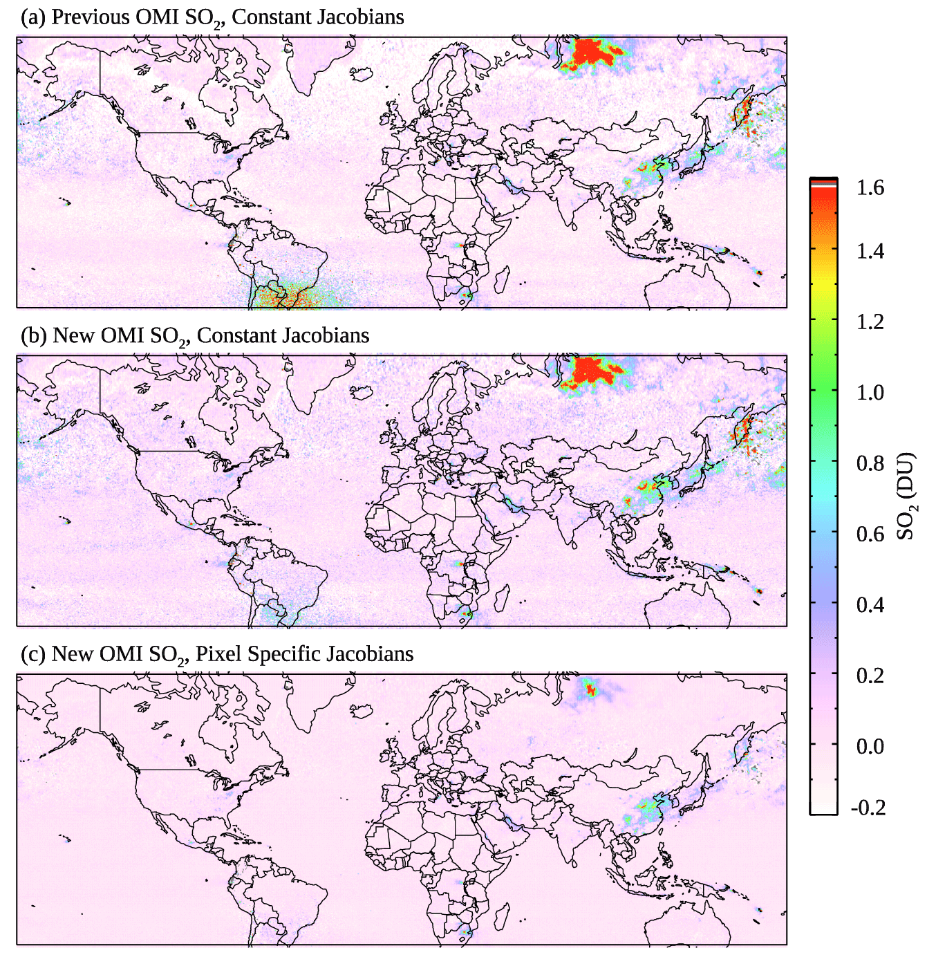
Figure 5 Monthly mean OMI SO₂ VCDs for May 2007 from (a) the previous PBL SO₂ dataset in OMSO2 V1.3 using constant Jacobians, (b) the new OMI anthropogenic SO₂ retrievals using the same Jacobians as in panel (a), and (c) the new OMI anthropogenic SO₂ dataset in OMSO2 V2 using pixel-specific Jacobians as described in Sect. 2.4. Data are gridded to a horizontal resolution of 0.25^∘ × 0.25^∘, and only those pixels near the center of the OMI swath (rows 6–55, 1-based), with SZA < 70^∘, and with a small cloud radiance fraction (CRF < 0.3) are included.

4.2 Retrievals over snow/ice

In Fig. 6, we examine the SO₂ VCDs over Norilsk, Russia, home to the world's largest anthropogenic SO₂ source (Norilsk Nickel smelters, Fioletov et al., 2016). The area is usually covered by snow/ice in April but not in July. As shown in Fig. 6c and d, there is a large seasonal change in SO₂ VCDs from the previous OMI PBL SO₂ dataset (OMSO2 V1.3), likely caused by snow/ice effects in April that were previously unaccounted for with the use of constant Jacobians. The maximal SO₂ VCD within the domain for April 2007 is 7.0 DU, a factor of 2 greater than the maximum of 3.5 DU for July of the same year. Similarly, the mean SO₂ VCD for April (0.14 DU) is over 3 times greater than that for July (0.04 DU). The temperature dependence of SO₂ cross sections may have also contributed to the apparent seasonal change here, but the effect is likely < 10 %. In comparison, the seasonal change in the new OMI anthropogenic SO₂ dataset (OMSO2 V2) over the same area is much smaller (Fig. 6a and b). The maximal SO₂ VCDs for the same 2 months are 2.5 and 3.4 DU, respectively, whereas the corresponding mean SO₂ VCDs are 0.07 and 0.04 DU. Note that the maximal and mean SO₂ VCDs for July are nearly identical between the two versions, implying that the updated retrievals over snow/ice are at least partly responsible for the more gradual and realistic seasonal change in OMSO2 V2.

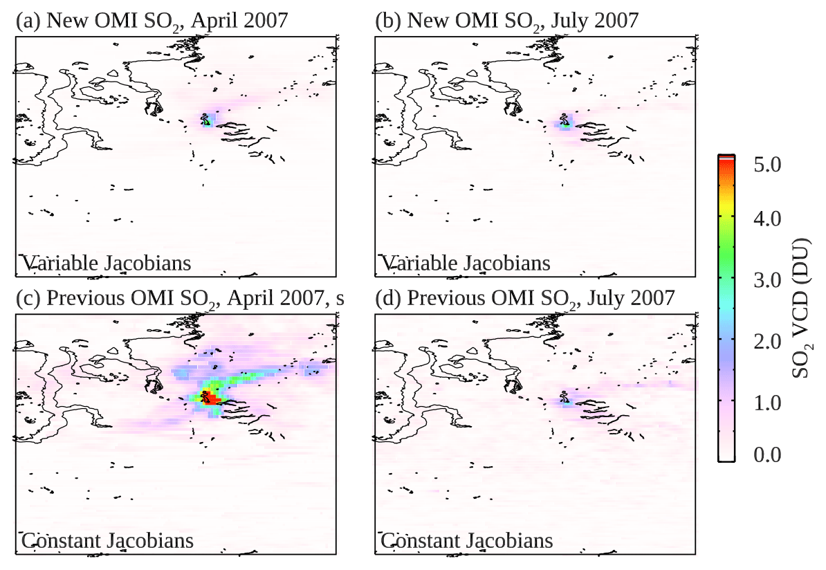
Figure 6 Monthly mean SO₂ VCDs from the new anthropogenic SO₂ dataset in OMSO2 V2 for (a) April and (b) July 2007 using pixel-specific Jacobians, showing comparable SO₂ over the area around Norilsk, Russia between the 2 months. Monthly mean SO₂ VCDs from the PBL SO₂ dataset in OMSO2 V1.3 show much greater apparent SO₂ in (c) April than in (d) July, due to the snow/ice effects that are unaccounted for with the constant Jacobians. Data have been filtered and gridded following the same criteria as in Fig. 5.

For another case of retrievals over snow/ice, refer to Fig. 7, which compares the new OMI anthropogenic SO₂ VCDs over snow-covered and snow-free surfaces during a historic snowstorm in eastern China in January to February 2008. Both Fig. 7a and b show retrievals from OMSO2 V2, but Fig. 7a is for retrievals over snow-covered pixels and Fig. 7b is for those over snow-free pixels. The two sets of retrievals are spatially well correlated (r=0.68), but retrievals over snow show generally stronger SO₂ signals over source areas that can be identified from the bottom-up emission inventory (Crippa et al., 2018) in Fig. 7c. This appears to provide evidence that highly reflective snow/ice surfaces can enhance OMI sensitivity to emission sources even at relatively large SZAs during wintertime, although a more thorough evaluation using other datasets such as those from ground monitors is necessary before a more definite conclusion can be drawn.

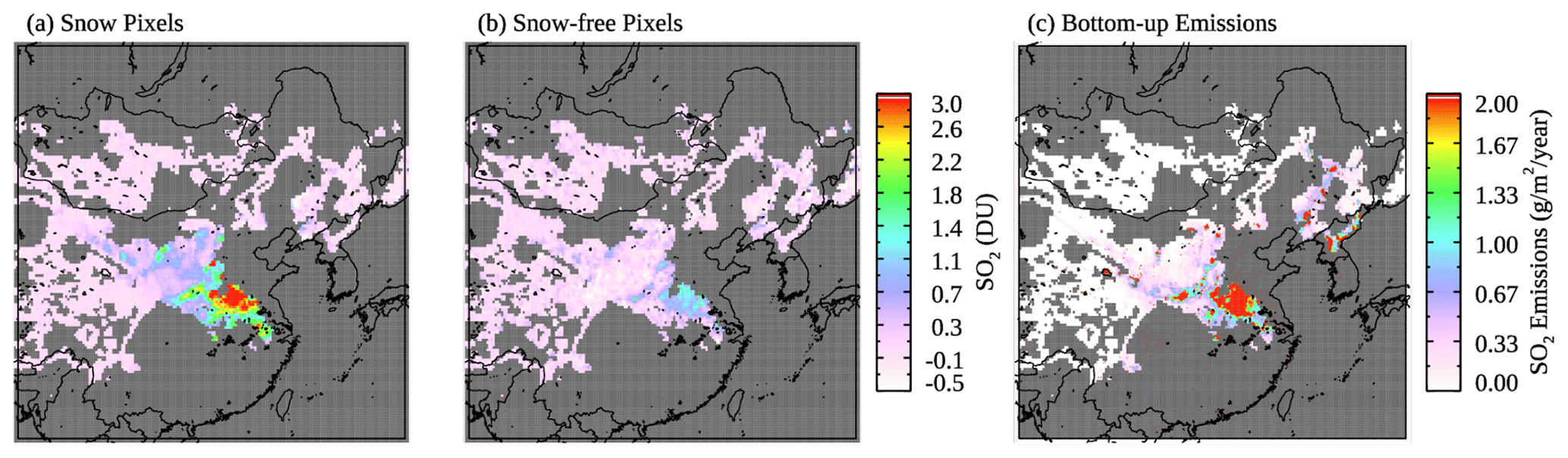
Figure 7 Mean SO₂ VCDs from the new anthropogenic SO₂ dataset in OMSO2 V2 for January to February 2008 over eastern China from pixels identified to be (a) cloud-free and covered by snow and (b) cloud-free (CRF < 0.1) and snow-free. Retrievals over snow pixels have enhanced signals over source areas that can be identified from (c) bottom-up emission estimates. Only grid cells having at least three observations from both snow and snow-free pixels during the 2-month period are shown.

4.3 Long-term regional trends in SO₂ VCDs

With stable retrievals over background areas (Sect. 3.2), the new OMI anthropogenic SO₂ dataset is particularly suitable for monitoring long-term regional trends in SO₂ pollution. Here we examine the changes in OMI SO₂ VCDs over two polluted regions, eastern China and India, from 2005 to 2019. To ensure consistent sampling throughout the entire period, we use data from the same set of OMI rows (6–24, 1-based) that are minimally affected by the row anomaly. Retrievals over snow/ice (Sect. 4.2) can enhance sensitivity to SO₂, but the sample size is too small for long-term data analysis for India and for most areas in China. As a result, we also focus on the warm season (April to October) when OMI has more retrievals and overall better sensitivity to SO₂, especially when compared with nonsnow days in the cold season. The results are presented in Fig. 8 for eastern China and in Fig. 9 for India. As shown in Fig. 8, SO₂ VCDs over China are much greater at the beginning of the OMI record than in recent years. We can also calculate the average total SO₂ mass within the domain by summing up the SO₂ mass from all grid cells that have SO₂ VCDs above a certain threshold. For grid cells with VCDs below the threshold, we assume that the actual SO₂ signal is too weak to be reliably detected by OMI, and we effectively treat them as if they contained no SO₂. Considering the typical retrieval noise (standard deviation) for a PBL SO₂ profile (∼ 0.5 DU) and the number of measurements during the 8-month period each year available for averaging (∼ 50–100), we chose 0.1 DU as a threshold. Calculated in this manner, the time series of SO₂ mass over China reached its peak at 27.5 kt in 2007 and then saw decreases in three consecutive years to the level of 15.6 kt in 2010, reflecting the effects of pollution control measures (Li et al., 2010) as well as the global financial crisis (Krotkov et al., 2016). The SO₂ mass rebounded to 20.0 kt in 2011 and remained relatively stable at around 16 kt, before starting to decrease sharply since 2014 to reach 5.7 kt in 2016 and 3.2 kt in 2019, marking a drastic drop of ∼ 88 % from the peak in 2007. As discussed in our previous study (Li et al., 2017a), such a large reduction in SO₂ over China is likely a result of major efforts undertaken by the Chinese government to address air quality issues. Given that the selection of the VCD threshold is somewhat arbitrary, we have also tested other thresholds. We found that adjusting the VCD threshold (e.g., to 0.05 DU) resulted in different estimates of the total mass (e.g., to 29.6, 18.3, 8.8, and 7.2 kt in 2007, 2010, 2016, and 2019, respectively) but did not significantly alter the overall relative trend. It also should be noted that the use of a threshold for total mass calculation can lead to biases. For example, for a background area where the retrieved VCDs are centered around zero, the use of a small positive threshold like 0.1 or 0.05 DU will likely cause a positive bias in the estimated SO₂ mass. It is thus important to carefully evaluate and characterize retrievals for a given region, before one can decide whether a threshold should be applied to mass calculation.

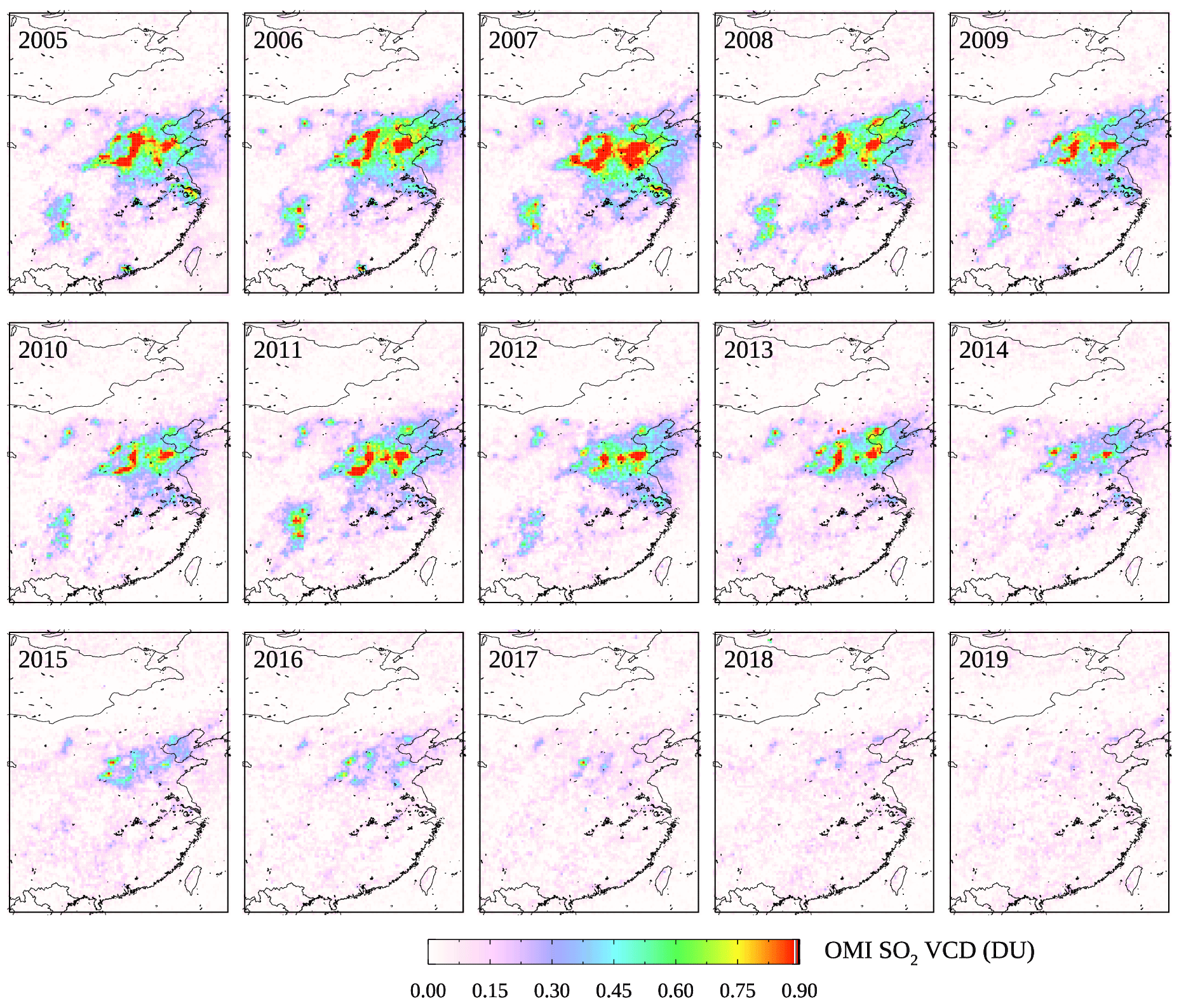
Figure 8 Mean warm season (April to October) OMI SO₂ VCDs over eastern China from the new anthropogenic SO₂ dataset in OMSO2 V2 for different years during 2005–2019. Data have been gridded to 0.25^∘ × 0.25^∘ resolution using pixels from OMI rows 6–24 (1-based) with cloud radiance fraction < 0.3, SZA < 65^∘, and AMF at 313 nm > 0.3. Mean SO₂ VCDs are calculated from the daily gridded data for each year, after excluding days potentially affected by large volcanic plumes.

For India, the trajectory of SO₂ pollution is quite different from that of China. The total SO₂ mass within the domain in Fig. 9 started at ∼ 1.2 kt in the first few years, increasing to 3.7 kt in 2016 and remaining at approximately at the same level for the next few years (e.g., 3.6 kt for 2019). Again, adjusting the VCD threshold from 0.1 to 0.05 DU changes the absolute amount of the estimated SO₂ mass (to ∼ 4 kt in 2005 and 2006, and 7.4 and 6.7 kt in 2016 and 2019, respectively), but the qualitative trend remains unchanged. The analysis here extends our previous study (Li et al., 2017a) and confirms the projection that India is indeed becoming the largest emitter of anthropogenic SO₂ in the world.

Figure 9 Same as Fig. 8 but for India.

5 Conclusions

We have made extensive updates to the PCA-based OMI anthropogenic SO₂ retrieval algorithm for the version 2 OMI SO₂ product (OMSO2 V2). The most important change involves the use of expanded lookup tables and model-based a priori vertical SO₂ profiles to account for the effects of various factors on SO₂ Jacobians for individual pixels, including observation geometry, ozone column amount and profile, cloud fraction and cloud pressure, surface pressure and reflectivity, and the vertical distribution of SO₂. Special consideration has also been given to retrievals over snow/ice. Other significant updates include new schemes that screen for pixels having relatively large volcanic or anthropogenic SO₂ signals to minimize their impacts on the PCA analysis and also an updated spectral fitting scheme that suppresses noise over the areas affected by the SAA.

Both spectral fitting and Jacobian calculations contribute to the uncertainties in the new OMI anthropogenic SO₂ retrievals. The contribution from the spectral fit part is represented by uncertainties in SCDs, which are largely driven by the signal-to-noise ratio of radiance measurements. This is evidenced by generally lower SCD uncertainties over clouds and snow/ice-covered surfaces and also at smaller SZAs. The SCD uncertainties on an individual pixel basis, estimated through both the fitting residuals and a statistical analysis, are ∼ 0.15–0.3 DU between ∼ 40^∘ S and ∼ 40^∘ N and ∼ 0.2–0.5 DU at higher latitudes. As for uncertainties in Jacobian calculations, the main contributions come from a priori profiles, cloud pressure, and the lack of explicit treatment for aerosol effects. The overall uncertainties in Jacobians are estimated at ∼ 50 %–100 % over polluted areas. For a mid-latitude pixel with an SO₂ SCD of ∼ 0.3 DU, typical of a moderately polluted area, the overall uncertainty in the VCD is ∼ 60 %–130 %.

The long-term stability of OMI anthropogenic SO₂ retrievals has also been assessed by examining the daily statistics of SCDs over the equatorial east Pacific. The mean and median SO₂ SCDs show little change throughout the 15-year data record from 2004 to 2019, increasing by ∼ 0.0035 and ∼ 0.003 DU, respectively. This highlights the remarkable stability of both OMI measurements and the PCA-based retrieval approach that intrinsically accounts for some of the instrument drifts. The standard deviation of SCDs, as a measure of retrieval noise, has increased by ∼ 0.02 DU or ∼ 10% since the beginning of the OMI mission, likely driven by more outliers in retrievals as suggested by the widening range between the 5th and 95th percentiles. Nonetheless, the annual increase in retrieval noise is well below 1 % and comparable with or slower than the growth of noise in OMI HCHO and NO₂ retrievals (Zara et al., 2018).

Comparisons with the previous OMI PBL SO₂ dataset in OMSO2 V1.3 show that the new algorithm leads to further improvements in data quality. When using the same Jacobians, the noise in VCDs over the equatorial Pacific is comparable between the two versions, but the updated spectral fit in V2 reduces the standard deviation in the monthly averaged VCDs over the SAA areas by about a third. The use of pixel-specific Jacobians further reduces retrieval noise over the background areas. Updated retrievals over snow/ice yield more gradual and realistic seasonal changes in SO₂ VCDs over the large source in Norilsk, Russia. Retrievals for snow-covered pixels over eastern China during a historic snowstorm in early 2008 also show enhanced signals over SO₂ sources, as compared with retrievals for snow-free pixels from the same period. Finally, SO₂ VCDs from the new anthropogenic SO₂ dataset show a continued reduction in SO₂ over eastern China since 2016 and a gradual overall increase over India from the beginning of the OMI record, confirming previous reports on the different trajectories of SO₂ pollution between the two countries.

In summary, the new OMI anthropogenic SO₂ dataset in OMSO2 V2 has several improvements over the previous PCA-based OMI PBL SO₂ dataset in OMSO2 V1.3. Looking forward, we are planning additional updates to the next version OMSO2 product. These include the use of daily a priori profiles from model simulations that better capture day-to-day variations in SO₂ vertical distribution, explicit consideration of aerosol effects on SO₂ Jacobians, and a more comprehensive error analysis for Jacobian calculations to assign an estimated VCD uncertainty for each pixel.