A channel selection method for hyperspectral atmospheric infrared sounders based on layering

This study introduces an effective channel selection method for hyperspectral infrared sounders. The method is illustrated for the Atmospheric InfraRed Sounder (AIRS) instrument. The results are as follows. (1) Using the improved channel selection (ICS), the atmospheric retrievable index is more stable, with the value reaching 0.54. The coverage of the weighting functions is more evenly distributed over height with this method. (2) Statistical inversion comparison experiments show that the accuracy of the retrieval temperature, using the improved channel selection method in this paper, is consistent with that of 1D-Var channel selection. In the stratosphere and mesosphere especially, from 10 to 0.02 hPa, the accuracy of the retrieval temperature of our improved channel selection method is improved by about 1 K. The accuracy of the retrieval temperature of ICS is also improved at lower heights. (3) Statistical inversion comparison experiments for four different regions illustrate latitudinal and seasonal variations and better performance of ICS compared to the numerical weather prediction (NWP) channel selection (NCS) and primary channel selection (PCS) methods. The ICS method shows potential for future applications.

1 Introduction

Since the successful launch of the first meteorological satellite, TIROS, in the 1960s, satellite observation technology has developed rapidly. Meteorological satellites observe the Earth's atmosphere from space and are able to record data from regions that are otherwise difficult to observe. Satellite data greatly enrich the content and range of meteorological observations, and, consequently, atmospheric exploration technology and meteorological observations have taken us to a new stage in our understanding of weather systems and related phenomena (Fang, 2014; Zhao et al., 2019). From the perspective of vertical atmospheric observation, satellite instruments are developing rapidly. In their infancy, the traditional infrared measurement instruments for detecting atmospheric temperature and moisture profiles, such as the TIROS Operational Vertical Sounder (TOVS) (Smith et al., 1991) or High Resolution Infrared Sounder (HIRS) in the Advanced TIROS Operational Vertical Sounder (ATOVS) (Chahine, 1972; Li et al., 2000; Liu, 2007), usually employed filter spectrometry. Even though such instruments have played an important role in improving weather prediction, it is difficult to continue to build upon improvements in terms of observation accuracy and vertical resolution due to the limitation of low spectral resolution. By using this kind of filter-based spectroscopic measurement instrument, therefore, it is difficult to meet today's needs in numerical weather prediction (Eyre et al., 1993; Prunet et al., 2010; Menzel et al., 2018). To meet this challenge, a series of plans for the creation of high-spectral-resolution atmospheric measurement instruments has been executed in the United States and in Europe in recent years. One example is the AIRS (Atmospheric InfraRed Sounder) on the Earth Observation System, “Aqua”, launched on 4 May 2002 from the United States. AIRS has 2378 spectral channels, providing sensitivity from the ground to up to about 65 km in altitude (Aumann et al., 2003; Hoffmann and Alexander, 2009; Gong et al., 2012). The United States and Europe, in 2010 and in 2012, also installed the CRIS (Cross-track Infrared Sounder) and the IASI (Infrared Atmospheric Sounding Interferometer) on polar-orbiting satellites, respectively.

China also places great importance on the development of such advanced sounding technologies. In the early 1990s, the National Satellite Meteorological Center began to investigate the principles and techniques of hyperspectral-resolution atmospheric observations. China's development of interferometric atmospheric vertical detectors eventually led to the launch of Fengyun no. 3 on 27 May 2008 and Fengyun no. 4 on 11 December 2016, both of which were equipped with infrared atmospheric instruments. How best to use the hyperspectral-resolution observation data obtained from these instruments, to obtain reliable atmospheric temperature and humidity profiles, is an active area of study in atmospheric inversion theory.

Due to technical limitations, at first only a limited number of channels could be built into the typical satellite instruments. In this case, channel selection generally involved controlling the channel weighting function by utilizing the spectral response characteristics of the channel (such as center frequency and bandwidth). With the development of measurement technology, increasing numbers of hyperspectral detectors were carried on meteorological satellites. Due to the large number of channels and data supported by such instruments today (such as AIRS with 2378 channels and IASI with 8461 channels), it has proven extremely cumbersome to store, transmit and process such data. Moreover, there is often a close correlation between the channel, causing an ill-posedness of the inversion and potentially compromising accuracy of the retrieval product based on hyperspectral-resolution data.

However, hyperspectral detectors have many channels and provide real-time mode prediction systems with vast quantities of data, which can significantly improve prediction accuracy. But if all the channels are used to retrieve data, the retrieval time considerably increases. Even more problematic are the glut of information produced and the unsuitability of the calculations for real-time forecasting. Concurrently, the computer processing power must be enough to meet the demands of simulating all the channels simultaneously within the forecast time. In order to improve the calculation efficiency and retrieval quality, it is very important to properly select a set of channels that can provide as much information as possible.

Many researchers have studied channel selection algorithms. Menke (1984) first chose channels using a data precision matrix method. Aires et al. (1999) made the selection using the Jacobian matrix, which has been widely used since then (Aires et al., 2002; Rabier et al., 2010). Rodgers (2000) indicated that there are two useful quantities in measuring the information provided by the observation data: Shannon information content and degrees of freedom. The concept of information capacity then became widely used in satellite channel selection. In 2007, Xu (2007) compared the Shannon information content with the relative entropy, analyzing the information loss and information redundancy. In 2008, Du et al. (2008) introduced the concept of the atmospheric retrievable index (ARI) as a criterion for channel selection, and, in 2010, Wakita et al. (2010) produced a scheme for calculating the information content of the various atmospheric parameters in remote sensing using Bayesian estimation theory. Kuai et al. (2010) analyzed both the Shannon information content and degrees of freedom in channel selection when retrieving CO₂ concentrations using thermal infrared remote sensing and indicated that 40 channels could contain 75 % of the information from the total channels. Cyril et al. (2003) proposed the optimal sensitivity profile method based on the sensitivity of different atmospheric components. Lupu et al. (2012) used degrees of freedom for signals (DFS) to estimate the amount of information contained in observations in the context of observing system experiments. In addition, the singular value decomposition method has also been widely used for channel selection (Prunet et al., 2010; Zhang et al., 2011; Wang et al., 2014). In 2017, Chang et al. (2017) selected a new set of Infrared Atmospheric Sounding Interferometer (IASI) channels using the channel score index (CSI). Richardson et al. (2018) selected 75 from 853 channels based on the high-spectral-resolution oxygen A-band instrument on NASA's Orbiting Carbon Observatory-2 (OCO-2), using information content analysis to retrieve the cloud optical depth, cloud properties and position.

Today's main methods for channel selection use only the weighting function to study appropriate numerical methods, such as the data precision matrix method (Menke, 1984), singular value decomposition method (Prunet et al., 2010; Zhang et al., 2011; Wang et al., 2014) and the Jacobi method (Aires et al., 1999; Rabier et al., 2010). The use of the methods allows sensitive channels to be selected. The above-mentioned studies also take into account the sensitivity of each channel to atmospheric parameters during channel selection, while ignoring some factors that impact retrieval results. The accuracy of retrieval results depends not only on the channel weighting function but also on the channel noise, background field and the retrieval algorithm.

Channel selection mostly uses the information content and delivers the largest amount of information for the selected channel combination during the retrieval (Rodgers, 1996; Du et al., 2008; He et al., 2012; Richardson et al., 2018).

This method has made great breakthroughs in both theory and practice, and the concept of information content itself does consider all the height dependencies of the kernel matrix K (Rodgers, 2000). However, earlier works have neglected the height dependencies of K for simplicity. This paper uses the atmospheric retrievable index (ARI) as the index, which is based on information content (Du et al., 2008; Richardson et al., 2018). Channel selection is made at different heights, and an effective channel selection scheme is proposed that fully considers various factors, including the influence of different channels on the retrieval results at different heights. This ensures the best accuracy of the retrieval product when using the selected channel. In addition, statistical inversion comparison experiments are used to verify the effectiveness of the method.

2 Channel selection indicator, scheme and method

2.1 Channel selection indicator

According to the concept of information content, the information content contained in a selected channel of a hyperspectral instrument can be described as H (Rodgers, 1996; Rabier et al., 2010). The final expression of H is as follows:

$$\begin{array}{}\text{(1)}& \begin{array}{rl}H& =-{\displaystyle \frac{\mathrm{1}}{\mathrm{2}}}\ln \left|\widehat{\mathbf{S}}{\mathbf{S}}_{\mathrm{a}}^{-\mathrm{1}}\right|\mathit{\epsilon },\\ & =-{\displaystyle \frac{\mathrm{1}}{\mathrm{2}}}\ln \left|\left({\mathbf{S}}_{\mathrm{a}}-{\mathbf{S}}_{\mathrm{a}}{\mathbf{K}}^T{\left({\mathbf{KS}}_{\mathrm{a}}{\mathbf{K}}^T+{\mathbf{S}}_{\mathit{\epsilon }}\right)}^{-\mathrm{1}}{\mathbf{KS}}_{\mathrm{a}}\right){\mathbf{S}}_{\mathrm{a}}^{-\mathrm{1}}\right|,\end{array}\end{array}$$

where S_a is the error covariance matrix of the background or the estimated value of atmospheric profile, S_ε represents the observation error covariance matrix of each hyperspectral detector channel, $\widehat{\mathbf{S}}=({\mathbf{S}}_{\mathrm{a}}-{\mathbf{S}}_{\mathrm{a}}{\mathbf{K}}^T{\left({\mathbf{KS}}_{\mathrm{a}}{\mathbf{K}}^T+{\mathbf{S}}_{\mathit{\epsilon }}\right)}^{-\mathrm{1}}{\mathbf{KS}}_{\mathrm{a}})$ denotes the covariance matrix after retrieval and K is the weighting function matrix.

In order to describe the accuracy of the retrieval results visually and quantitatively, the atmospheric retrievable index (ARI), p, (Du et al., 2008) is defined as follows:

$$\begin{array}{}\text{(2)}& p=\mathrm{1}-\exp \left({\displaystyle \frac{\mathrm{1}}{\mathrm{2}n}}\ln \left|\widehat{\mathbf{S}}{\mathbf{S}}_{\mathrm{a}}^{-\mathrm{1}}\right|\right).\end{array}$$

Assuming that before and after the retrieval the ratio of the root-mean-square error of each element in the atmospheric state vector is 1−p, then $\left|\widehat{\mathbf{S}}{\mathbf{S}}_{\mathrm{a}}^{-\mathrm{1}}\right|=(\mathrm{1}-p{)}^{\mathrm{2}n}$ is derived. By inverting the equation, the ARI that is p can be obtained in Eq. (2), which indicates the relative portion of the error that is eliminated by retrieval. In fact, before and after retrieval, the ratio of the root-mean-square error of each element cannot be 1−p. Therefore, p defined by Eq. (1) is actually an overall evaluation of the retrieval result.

2.2 Channel selection scheme

The principle of channel selection is to find the optimum channel combination after numbering the channels. This combination makes the information content, H, or the ARI defined in this paper as large as possible, in order to maintain the highest possible accuracy in the retrieval results.

There are M layers in the vertical direction of the atmosphere and N satellite channels. Selecting n from N channels, there will be $C_N^n$ combinations in each layer, leading $C_N^n$ calculations to get $C_N^n$ kinds of p results. Furthermore, there are M layers in the vertical direction of the atmosphere. Therefore, the entire atmosphere must be calculated $M\cdot C_N^n$ times. However, the calculation $M\cdot C_N^n$ times will be particularly large, which makes this approach impractical in calculating p for all possible combinations. Therefore, it is necessary to design an effective calculation scheme, and such a scheme, i.e., a channel selection method, using iteration is proposed, called the “sequential absorption method” (Dudhia et al., 2002; Du et al., 2008). The method's main function is to select (“absorb”) channels one by one, taking the channel with the maximum value of p. Through n iterations, n channels can be selected as the final channel combination. The steps are as follows:

(I) The expression of information content in a single channel.

First, we use only one channel for retrieval. A row vector, k, in the weighting function matrix, K, is a weighting function corresponding to the channel. After observation in this channel, the error covariance matrix is as follows:

$$\begin{array}{}\text{(3)}& \widehat{\mathbf{S}}={\mathbf{S}}_{\mathrm{a}}-{\mathbf{S}}_{\mathrm{a}}{\mathit{k}}^T{\left(s_{\mathit{\epsilon }}+\mathit{k}{\mathbf{S}}_{\mathrm{a}}{\mathit{k}}^T\right)}^{-\mathrm{1}}\mathit{k}{\mathbf{S}}_{\mathrm{a}}.\end{array}$$

It should be noted that (s_ε+kS_ak^T) is a scalar value in Eq. (3), thus Eq. (3) can be converted to the following equation:

$$\begin{array}{}\text{(4)}& \widehat{\mathbf{S}}=\left(I-{\displaystyle \frac{{\mathbf{S}}_{\mathrm{a}}{\mathit{k}}^T\mathit{k}}{\left(s_{\mathit{\epsilon }}+\mathit{k}{\mathbf{S}}_{\mathrm{a}}{\mathit{k}}^T\right)}}\right){\mathbf{S}}_{\mathrm{a}}=\left(I-{\displaystyle \frac{(\mathit{k}{\mathbf{S}}_{\mathrm{a}}{)}^T\mathit{k}}{\left(s_{\mathit{\epsilon }}+\mathit{k}(\mathit{k}{\mathbf{S}}_{\mathrm{a}}{)}^T\right)}}\right){\mathbf{S}}_{\mathrm{a}}.\end{array}$$

Substituting Eq. (4) into Eq. (2) gives the following equation:

$$\begin{array}{}\text{(5)}& p=\mathrm{1}-\exp \left({\displaystyle \frac{\mathrm{1}}{\mathrm{2}n}}\ln \left(\left|I-{\displaystyle \frac{(\mathit{k}{\mathbf{S}}_{\mathrm{a}}{)}^T\mathit{k}}{\left(s_{\mathit{\epsilon }}+\mathit{k}(\mathit{k}{\mathbf{S}}_{\mathrm{a}}{)}^T\right)}}\right|\right)\right).\end{array}$$

(II) Simplification of Eq. (5) for calculating the p value.

Since S_a and S_ε are positive definite symmetric matrices, they can be decomposed into ${\mathbf{S}}_{\mathrm{a}}=\left({\mathbf{S}}_{\mathrm{a}}^{\mathrm{1}/\mathrm{2}}{)}^T\right({\mathbf{S}}_{\mathrm{a}}^{\mathrm{1}/\mathrm{2}})$ and ${\mathbf{S}}_{\mathit{\epsilon }}=\left({\mathbf{S}}_{\mathit{\epsilon }}^{\mathbf{1}/\mathbf{2}}{)}^{\mathbf{T}}\right({\mathbf{S}}_{\mathit{\epsilon }}^{\mathbf{1}/\mathbf{2}})$.

This can be defined using the following equation:

$$\begin{array}{}\text{(6)}& \mathbf{R}={\mathbf{S}}_{\mathit{\epsilon }}^{\mathrm{1}/\mathrm{2}}{\mathbf{KS}}_{\mathrm{a}}^{\mathrm{1}/\mathrm{2}}.\end{array}$$

The matrix R can then be regarded as a weighting function matrix, normalized by the observed error and a priori uncertainty. A row vector of R, $r=s_{\mathit{\epsilon }}^{-\mathrm{1}/\mathrm{2}}\mathit{k}{\mathbf{S}}_{\mathrm{a}}^{\mathrm{1}/\mathrm{2}}$, represents the normalized weighting function matrix of a single channel. Substituting r into Eq. (5) gives the following equation:

$$\begin{array}{}\text{(7)}& p=\mathrm{1}-\exp \left({\displaystyle \frac{\mathrm{1}}{\mathrm{2}n}}\ln \left(\left|I-{\displaystyle \frac{r{r}^T}{\mathrm{1}+r^{T}r}}\right|\right)\right).\end{array}$$

For arbitrary row vectors, a and b, using the matrix property $\det \left(I+a^{T}b\right)=\mathrm{1}+b{a}^T$, the new expression for p is as follows:

$$\begin{array}{}\text{(8)}& \begin{array}{rl}p& =\mathrm{1}-\exp \left({\displaystyle \frac{\mathrm{1}}{\mathrm{2}n}}\ln \left(\mathrm{1}-{\displaystyle \frac{r^{T}r}{\mathrm{1}+r^{T}r}}\right)\right)\\ & =\mathrm{1}-\exp \left({\displaystyle \frac{\mathrm{1}}{\mathrm{2}n}}\ln \left({\displaystyle \frac{\mathrm{1}}{\mathrm{1}+r^{T}r}}\right)\right)\\ & =\mathrm{1}-\exp \left(-{\displaystyle \frac{\mathrm{1}}{\mathrm{2}n}}\ln \left(\mathrm{1}+r^{T}r\right)\right).\end{array}\end{array}$$

(III) Iteration in a single layer.

First, the iteration in a single layer requires the calculation of R. Using S_a, S_ε , K and Eq. (6), R can be calculated. Second, using Eq. (8), p of each candidate channel can be calculated. Moreover, the channel corresponding to maximum p is the selected channel for this iteration. After a channel has been selected, according to Eq. (3) we can use $\widehat{\mathbf{S}}$ to get S_a for the next iteration. Finally, channels which are not selected during this iteration are used as the candidate channels for the next iteration.

When selecting n from N channels, it is necessary to calculate $(N-n/\mathrm{2})n\approx Nnp$ values, which is much smaller than $C_N^n$. In addition to high computational efficiency by using this method, another advantage is that all channels can be recorded in the order in which they are selected. In the actual application, if n^′ channels are needed and $n^{\prime }<n$, we will not need to select the channel again but record the selected channel only.

(IV) Iteration for different altitudes.

Because satellite channel sensitivity varies with height, repeating the iterative process of step (III) selects the optimum channels at different heights. Assuming there are M layers in the atmosphere and selecting n from N channels, it is necessary to calculate $M\cdot (N-n/\mathrm{2})n\approx M\cdot Nnp$ values, a much smaller number than $M\cdot C_N^n$. In this way, different channel sets can be used to evaluate corresponding height in the retrieved profiles.

2.3 Statistical inversion method

The inversion methods for the atmospheric temperature profiles can be summarized in two categories: statistical inversion and physical inversion. Statistical inversion is essentially a linear regression model, which uses a large number of satellite measurements and atmospheric parameters to match samples and calculate their correlation coefficient. Then, based on the correlation coefficient, the required parameters of the independent measurements obtained by the satellite are retrieved. Because the method does not directly solve the radiation transfer equation, it has the advantage of fast calculation speed. In addition, the solution is numerically stable, which makes it one of the highest-precision methods (Chedin et al., 1985). Therefore, the statistical inversion method will be used for our channel selection experiment and a regression equation will be established.

According to an empirical orthogonal function, the atmospheric temperature (or humidity), T, and the brightness temperature, T_b, are expanded as follows:

$$\begin{array}{}\text{(9)}& {\displaystyle }& {\displaystyle }\mathbf{T}={\mathbf{T}}^{\ast }\cdot \mathbf{A},\text{(10)}& {\displaystyle }& {\displaystyle }{\mathbf{T}}_{\mathbf{b}}={\mathbf{T}}_{\mathbf{b}}^{\ast }\cdot \mathbf{A},\end{array}$$

where T^∗ and ${\mathbf{T}}_{\mathbf{b}}^{\ast }$ are the eigenvectors of the covariance matrix of temperature (or humidity) and brightness temperature, respectively. A and B stand for the corresponding expansion coefficient vectors of temperature (humidity) and brightness temperature.

Using the least-squares method and the orthogonal property, the coefficient conversion matrix, V, is introduced:

$$\begin{array}{}\text{(11)}& \mathbf{A}=\mathbf{V}\cdot \mathbf{A},\end{array}$$

where

$$\begin{array}{}\text{(12)}& \mathbf{V}={\mathbf{AB}}^{\mathbf{T}}{\left({\mathbf{BB}}^{\mathbf{T}}\right)}^{-\mathrm{1}}.\end{array}$$

Using the orthogonality, we get the following equation:

$$\begin{array}{}\text{(13)}& {\displaystyle }& {\displaystyle }\mathbf{B}=({\mathbf{T}}_{\mathbf{b}}^{\ast }{)}^{\mathbf{T}}{\mathbf{T}}_{\mathbf{b}},\text{(14)}& {\displaystyle }& {\displaystyle }\mathbf{A}=({\mathbf{T}}^{\ast }{)}^{\mathbf{T}}\mathbf{T}.\end{array}$$

For convenience, the anomalies of the state vector (atmospheric temperature), T, and the observation vector (brightness temperature), T_b, are taken as follows:

$$\begin{array}{}\text{(15)}& \widehat{\mathbf{T}}=\stackrel{\mathrm{‾}}{\mathbf{T}}+{\widehat{\mathbf{T}}}^{\prime }=\stackrel{\mathrm{‾}}{\mathbf{T}}+{\mathbf{GT}}_{\mathbf{b}}^{\prime }=\stackrel{\mathrm{‾}}{\mathbf{T}}+\mathbf{G}\left({\mathbf{T}}_{\mathbf{b}}-\stackrel{\mathrm{‾}}{{\mathbf{T}}_{\mathbf{b}}}\right),\end{array}$$

where $\widehat{\mathbf{T}}$ stands for the retrieval atmospheric temperature. $\stackrel{\mathrm{‾}}{\mathbf{T}}$ and $\stackrel{\mathrm{‾}}{{\mathbf{T}}_{\mathbf{b}}}$ are the corresponding average values of the elements, respectively. ${\widehat{\mathbf{T}}}^{\prime }$ and ${{\mathbf{T}}_{\mathbf{b}}}^{\prime }$ represent the corresponding anomalies of the elements, respectively.

Assuming there are k sets of observations, a sample anomaly matrix with k vectors can be constructed:

$$\begin{array}{}\text{(16)}& {\displaystyle }& {\displaystyle }{\mathbf{T}}^{\prime }=(t_{\mathrm{1}}^{\prime },t_{\mathrm{2}}^{\prime },\mathrm{\dots },t_k^{\prime }),\text{(17)}& {\displaystyle }& {\displaystyle }{\mathbf{T}}_{\mathbf{b}}^{\prime }=(t_{b\mathrm{1}}^{\prime },t_{b\mathrm{2}}^{\prime },\mathrm{\dots },t_{bk}^{\prime }).\end{array}$$

Define the inversion error matrix as follows:

$$\begin{array}{}\text{(18)}& \mathit{\delta }=\stackrel{\mathrm{‾}}{\mathbf{T}}-\widehat{\mathbf{T}}={\widehat{\mathbf{T}}}^{\prime }-{\mathbf{T}}^{\prime }.\end{array}$$

The retrieval error covariance matrix is as follows:

$$\begin{array}{}\text{(19)}& \begin{array}{rl}{\mathbf{S}}_{\mathit{\delta }}& ={\displaystyle \frac{\mathrm{1}}{k-n-\mathrm{1}}}\mathit{\delta }{\mathit{\delta }}^{\mathbf{T}},\\ & ={\displaystyle \frac{\mathrm{1}}{k-n-\mathrm{1}}}({\mathbf{T}}^{\prime }-{\mathbf{GT}}_{\mathbf{b}}^{\prime })({\mathbf{T}}^{\prime }-{\mathbf{GT}}_{\mathbf{b}}^{\prime }{)}^{\mathbf{T}},\\ & ={\displaystyle \frac{k-\mathrm{1}}{k-n-\mathrm{1}}}({\mathbf{S}}_{\mathbf{e}}-{\mathbf{G}}^{\mathbf{T}}{\mathbf{S}}_{\mathbf{xy}}-{\mathbf{S}}_{\mathbf{xy}}{\mathbf{G}}^{\mathbf{T}}+{\mathbf{GS}}_{\mathbf{y}}{\mathbf{G}}^{\mathbf{T}}),\end{array}\end{array}$$

where

$$\begin{array}{}\text{(20)}& \begin{array}{rl}& {\mathbf{S}}_e={\displaystyle \frac{\mathrm{1}}{k-\mathrm{1}}}{\mathbf{T}}^{\prime }{{\mathbf{T}}^{\prime }}^{\mathbf{T}},\\ & {\mathbf{S}}_y={\displaystyle \frac{\mathrm{1}}{k-\mathrm{1}}}{\mathbf{T}}_{\mathbf{b}}^{\prime }{{\mathbf{T}}_{\mathbf{b}}^{\prime }}^{\mathbf{T}},\\ & {\mathbf{S}}_{xy}={\displaystyle \frac{\mathrm{1}}{k-\mathrm{1}}}{\mathbf{T}}^{\prime }{{\mathbf{T}}_{\mathbf{b}}^{\prime }}^{\mathbf{T}}.\end{array}\end{array}$$

S_e stands for the sample covariance matrix of T, S_y denotes the sample covariance matrix of T_b, and S_xy represents the covariance matrix of T and T_b. The elements on the diagonal of the error covariance matrix, S_δ, represent the retrieval error variance of T. The matrix G that minimizes the overall error variance is the least-squares coefficient matrix of the regression Eq. (15), which meets the following criterion:

$$\begin{array}{}\text{(21)}& {\mathit{\delta }}^{\mathrm{2}}=\mathrm{tr}\left({\mathbf{S}}_{\mathit{\delta }}\right)=\min .\end{array}$$

Taking a derivative of Eq. (21) with respect to G, $\frac{\partial }{\partial \mathbf{G}}\mathrm{tr}\left({\mathbf{S}}_{\mathit{\delta }}\right)=\mathrm{0}=(-\mathrm{2}{\mathbf{S}}_{xy}+\mathrm{2}{\mathbf{GS}}_y)$, which means that

$$\begin{array}{}\text{(22)}& \mathbf{G}={\mathbf{S}}_{xy}{\mathbf{S}}_y^{-\mathrm{1}}.\end{array}$$

Substituting Eq. (22) into Eq. (15) finally gives the least-squares solution as follows:

$$\begin{array}{}\text{(23)}& \widehat{\mathbf{T}}=\stackrel{\mathrm{‾}}{\mathbf{T}}+{\mathbf{S}}_{xy}{\mathbf{S}}_y^{-\mathrm{1}}\left({\mathbf{T}}_{\mathbf{b}}-\stackrel{\mathrm{‾}}{{\mathbf{T}}_{\mathbf{b}}}\right).\end{array}$$

It should be noted that the least-squares solution obtained here aims to minimize the sum of the error variance for each element in the atmospheric state vector after retrieval for several different times. At present, statistical multiple regression is widely used in the retrieval of atmospheric profiles based on atmospheric remote sensing data. As long as there are enough data, S_xy and S_y can be determined.

3 Channel selection experiment

3.1 Data and model

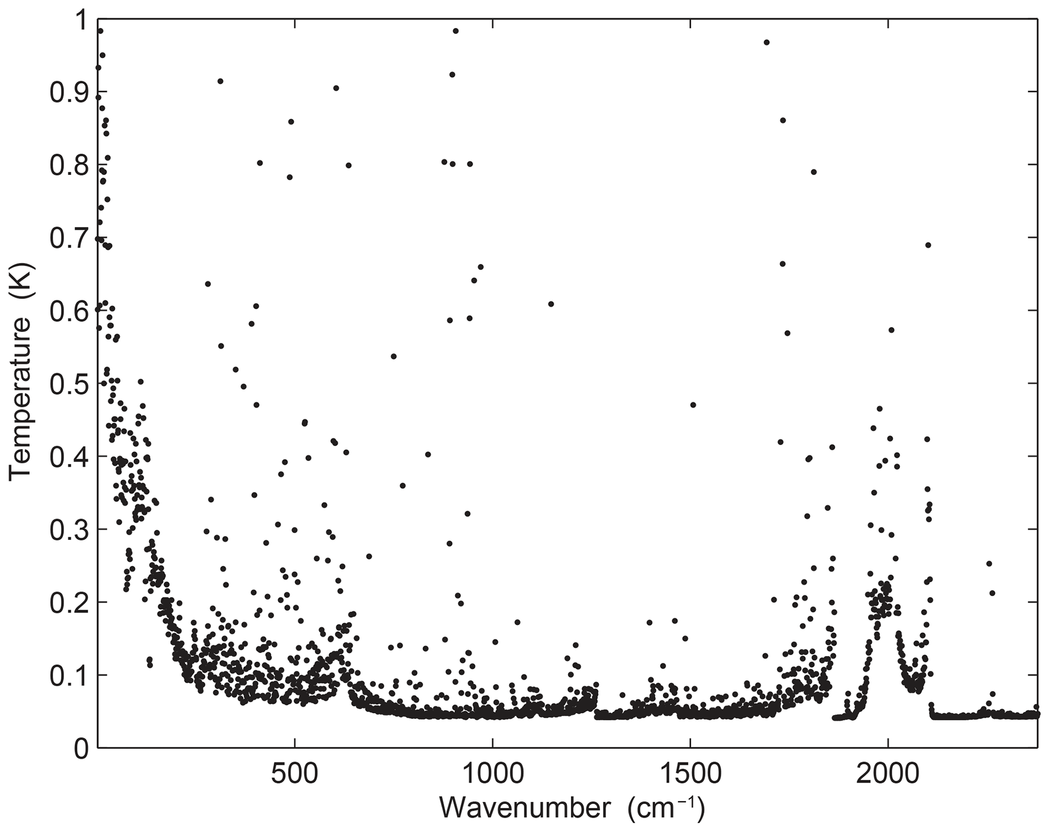
The Atmospheric Infrared Sounder (AIRS) is primarily designed to measure the Earth's atmospheric water vapor and temperature profiles on a global scale (Aumann et al., 2003; Susskind et al., 2003). AIRS is a continuously operating cross-track-scanning sounder, consisting of a telescope that feeds an echelle spectrometer. The AIRS infrared spectrometer acquires 2378 spectral samples at a resolution λ∕Δλ, ranging from 1086 to 1570, in three bands: 3.74 to 4.61, 6.20 to 8.22 and 8.8 to 15.4 µm. The footprint size is 13.5 km. The spectral range includes 4.3 and 15.5 µm for important temperature observation and CO₂, 6.3 µm for water vapor, and 9.6 µm for ozone absorption bands (Menzel et al., 2018). The root-mean-square error (RMSE) of the measured radiation is better than 0.2 K (Susskind et al., 2003). Moreover, global atmospheric profiles can be detected every day. Due to radiometer noise and faults, there are currently only 2047 effective channels. However, compared with previous infrared detectors, AIRS boasts a significant improvement in both the number of channels and spectral resolution (Aumann, 1994; Huang et al., 2005; Li et al., 2005).

The root-mean-square error of an AIRS infrared channel is shown in Fig. 1. The measurement error is not below 0.2 K for all the instrument channels. There are a few channels with extremely large measurement errors, which reduce the accuracy of prediction to some extent. Among them, some extremely large measurement errors reduce the accuracy of prediction to some extent (Susskind et al., 2003). At present, more than 300 channels have not been used because their errors exceed 1 K. If data from these channels were to be used for retrieval, the accuracy of the retrieval could be reduced. Therefore, it is necessary to select a group of channels to improve the calculation efficiency and retrieval quality. In this paper we study channel selection for temperature profile retrieval by AIRS.

Figure 1 Root-mean-square error of AIRS infrared channel (black spots).

For the calculation of radiative transfer and the weighting function matrix, K, the RTTOV (Radiative Transfer for TIROS Operational Vertical Sounder) v12 fast radiative transfer model is used. Although initially developed for the TOVS (TIROS Operational Vertical Sounder) radiometers, RTTOV can now simulate around 90 different satellite sensors measuring in the MW (microwave), IR (infrared) and VIS (visible) regions of the spectrum (Saunders et al., 2018). The model allows rapid simulations (1 ms for 40 channel Advanced TOVS, ATOVS, on a desktop PC) of radiances for satellite visible, infrared, or microwave nadir-scanning radiometers given atmospheric profiles of temperature and trace gas concentrations and cloud and surface properties. The only mandatory gas included as a variable for RTTOV v12 is water vapor. Optionally, ozone, carbon dioxide, nitrous oxide, methane, carbon monoxide and sulfur dioxide can be included, with all other constituents assumed to be constant. RTTOV can accept input profiles on any defined set of pressure levels. The majority of RTTOV coefficient files are based on the 54 levels (see Table A1 in Appendix A), in the range from 1050 to 0.01 hPa, though coefficients for some hyperspectral sounders are also available on 101 levels.

In order to correspond to the selected profiles, the atmosphere is divided into 137 layers, each of which contains corresponding atmospheric characteristics, such as temperature, pressure and the humidity distribution. Each element in the weighting function matrix can be written as $\partial yi/\partial xj$. The subscript i is used to identify the satellite channel, and the subscript j is used to identify the atmospheric variable. Therefore, $\partial yi/\partial xj$ indicates the variation in brightness temperature in a given satellite channel, when a given atmospheric variable in a given layer changes. We are thus able to establish which layer of the satellite channel is particularly sensitive to which atmospheric characteristic (temperature, various gas contents) in the vertical atmosphere. The RTTOV_K (the K mode) is used to calculate the matrix H(X0) (Eq. 1) for a given atmospheric profile characteristic.

3.2 Channel selection comparison experiment and results

In order to verify the effectiveness of the method, three sets of comparison experiments were conducted. First, 324 channels used by the EUMETSAT Satellite Application Facility on Numerical Weather Prediction (NWP-SAF) were selected. NCS is short for NWP channel selection in this paper. NCSs were released by the NWP-SAF 1D-Var (one-dimensional variational analysis) scheme, in accordance with the requirements of the NWP-SAF (Saunders et al., 2018). Second, 324 channels were selected using the information capacity method. This method was adopted by Du et al. (2008) without the consideration of layering. PCS is short for primary channel selection in this paper.

Figure 2 Error covariance matrix of temperature (shaded).

Third, 324×M channels were selected using the information capacity method for the M layer atmosphere. ICS is short for improved channel selection in this paper. In order to verify the retrieval effectiveness after channel selection, statistical inversion comparison experiments were performed using 5000 temperature profiles provided by the ECMWF dataset, which will be introduced in Sect. 4.

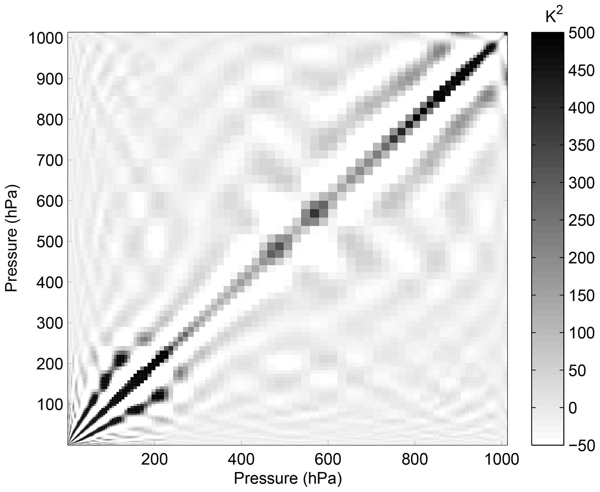
The observation error covariance matrix, S_ε, in the experiment is provided by NWP-SAF 1D-Var. In general, it can be converted to a diagonal matrix, the elements of which are the observation error standard deviation of each hyperspectral detector channel, which is the square of the root-mean-square error for each channel. The root-mean-square error of the AIRS channels is shown in Fig. 1. The error covariance matrix of the background, S_a, is calculated using 5000 samples of the IFS-137 data provided by the ECMWF dataset (The detailed information will be introduced in Sect. 4). The last access date is 26 April 2019 (download address: https://www.nwpsaf.eu/site/update-137-level-nwp-profile-dataset/ last access: 11 January 2020). The covariance matrix of temperature is shown in Fig. 2. The results are consistent with the previous study by Du et al. (2008).

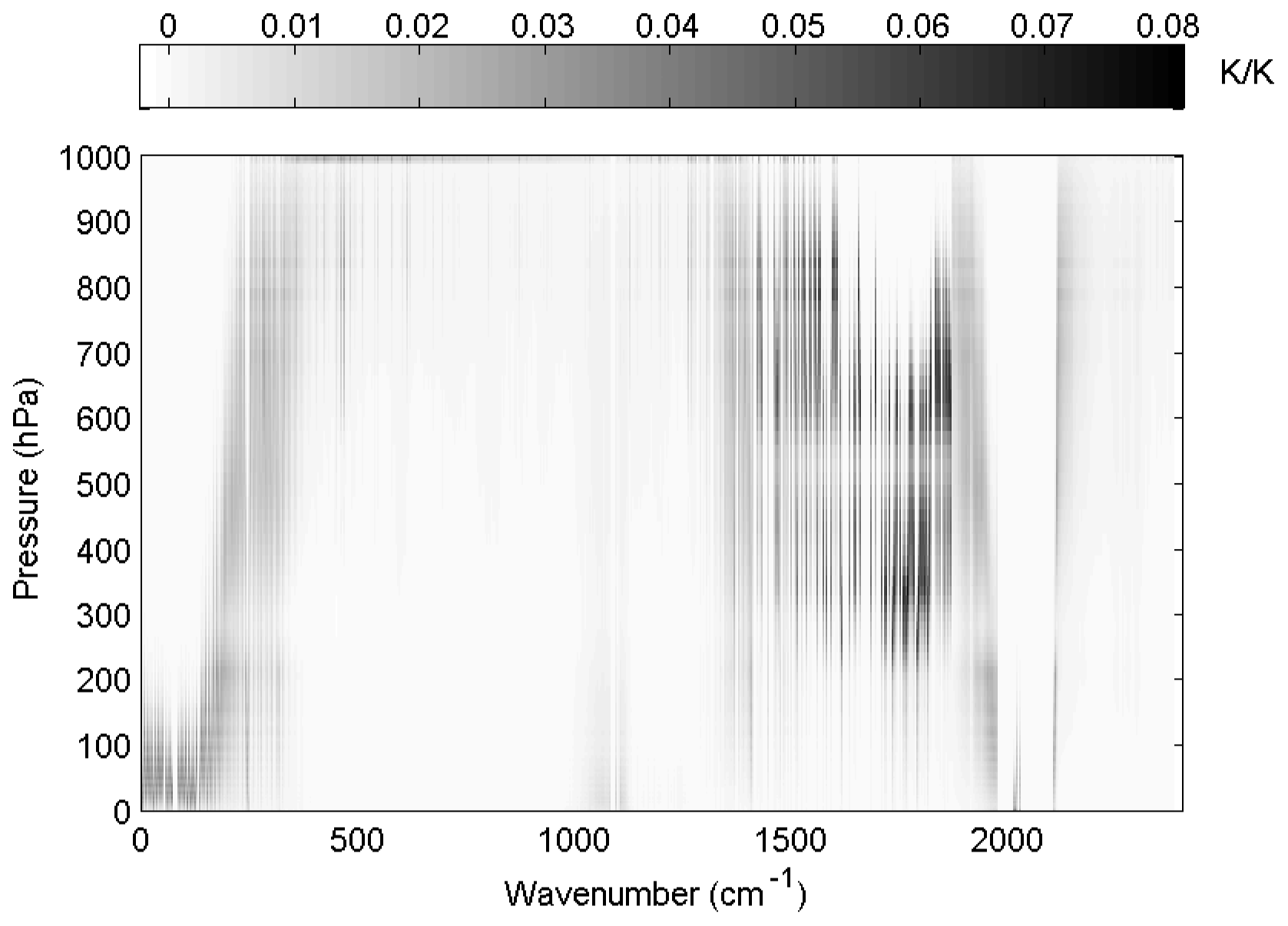
The reference atmospheric profiles are from the IFS-137 database, and the temperature weighting function matrix is calculated using the RTTOV_K mode, as shown in Fig. 3; the results are consistent with those of the previous study by Du et al. (2008). For the air-based passive atmospheric remote sensing studied in this paper, when the same channel detects the atmosphere from different observation angles, the value of the weighting function matrix K changes due to the limb effect. The goal of this section is focusing on the selection methods of selecting channels; therefore, the biases produced from different observation angles can be ignored.

Figure 3 Temperature weighting function matrix (shaded).

In order to verify the effectiveness of the method, the distribution of 324 channels in the AIRS brightness temperature spectrum, without considering layering, is indicated in Fig. 4. The background brightness temperature is the simulated AIRS observation brightness temperature, which is from the atmospheric profile in RTTOV put into the model. Figure 4a shows the 324 channels selected by PCS, while Fig. 4b shows the 324 channels selected by NCS.

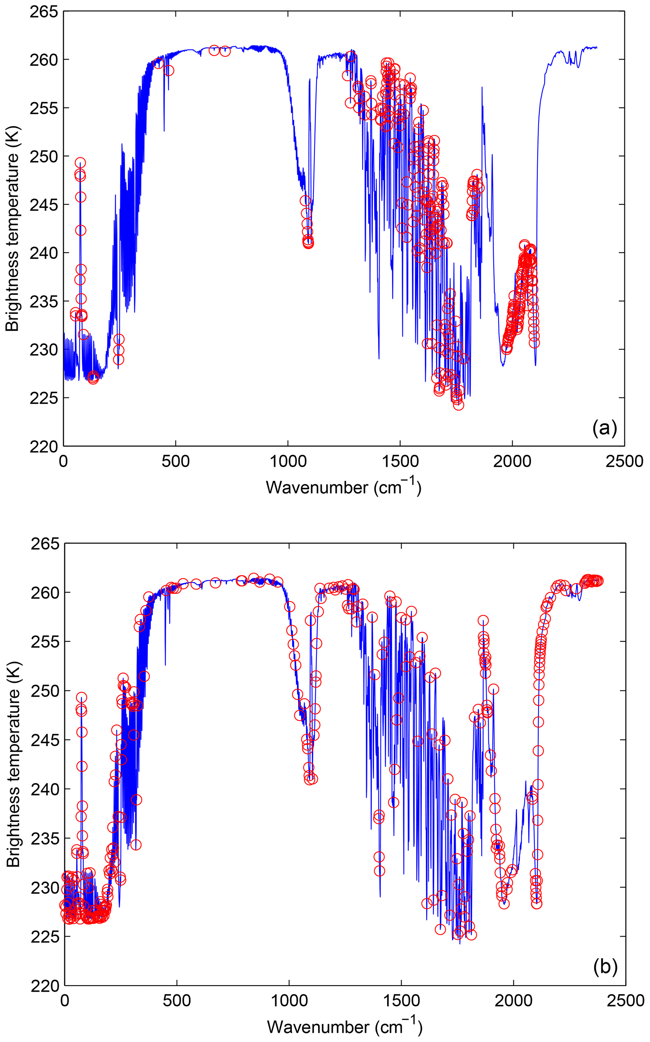
Figure 4 The distribution of different channel selection methods without considering layering in the AIRS brightness temperature spectrum (blue line): (a) 324 channels selected by PCS (red circles) and (b) 324 channels selected by NCS (red circles).

Without considering layering, the main differences between the 324 channels selected by PCS and NCS are as follows. (1) In the near 10 µm band, fewer channels are selected by PCS because the retrieval of ground temperature is considered by NCS. (2) In the near 9 µm band, no channels are selected by PCS because the retrieval of O₃ is not considered in this paper. (3) As is known, the spectral range from 6 to 7 µm corresponds to water vapor absorption bands, but fewer channels are selected by NCS; (4) Near 5 µm band, it includes 4.2 µm for N₂O and 4.3 µm for CO₂ absorption bands. As is shown in Fig. 4, fewer channels are selected by PCS in those bands. PCS is favorable for atmospheric temperature observation. Because 4.2 and 4.3 µm bands are sensitive to high temperature, a better observation can be obtained for higher temperatures. (5) In the near 4 µm band, a small number of channels are selected by NCS, but no channels are selected by PCS.

Above all, the information content considered in this study only takes the temperature profile retrieval into consideration, thus the channel combination of PCS is inferior to that of NCS for the retrieval of surface temperature and the O₃ profile. The advantages of the channel selection method based on information content in this paper are mainly reflected in the following ways: (1) the stratosphere and mesosphere are less affected by the ground surface, thus the retrieval result of PCS is better than that of NCS. (2) Due to the method selected in this paper there are more channels at 4.2 µm for N₂O and 4.3 µm for CO₂ absorption bands. The channel combination of PCS is better than that of NCS for atmospheric temperature observation at higher temperature.

By comparing channel selection without considering layering, we note the general advantages and disadvantages of PCS and NCS for the retrieval of temperature and can improve the channel selection scheme. First, the retrieval of the temperature profile for 324 channels selected by PCS is obtained. The relationship between the number of iterations and the ARI is shown in Fig. 5.

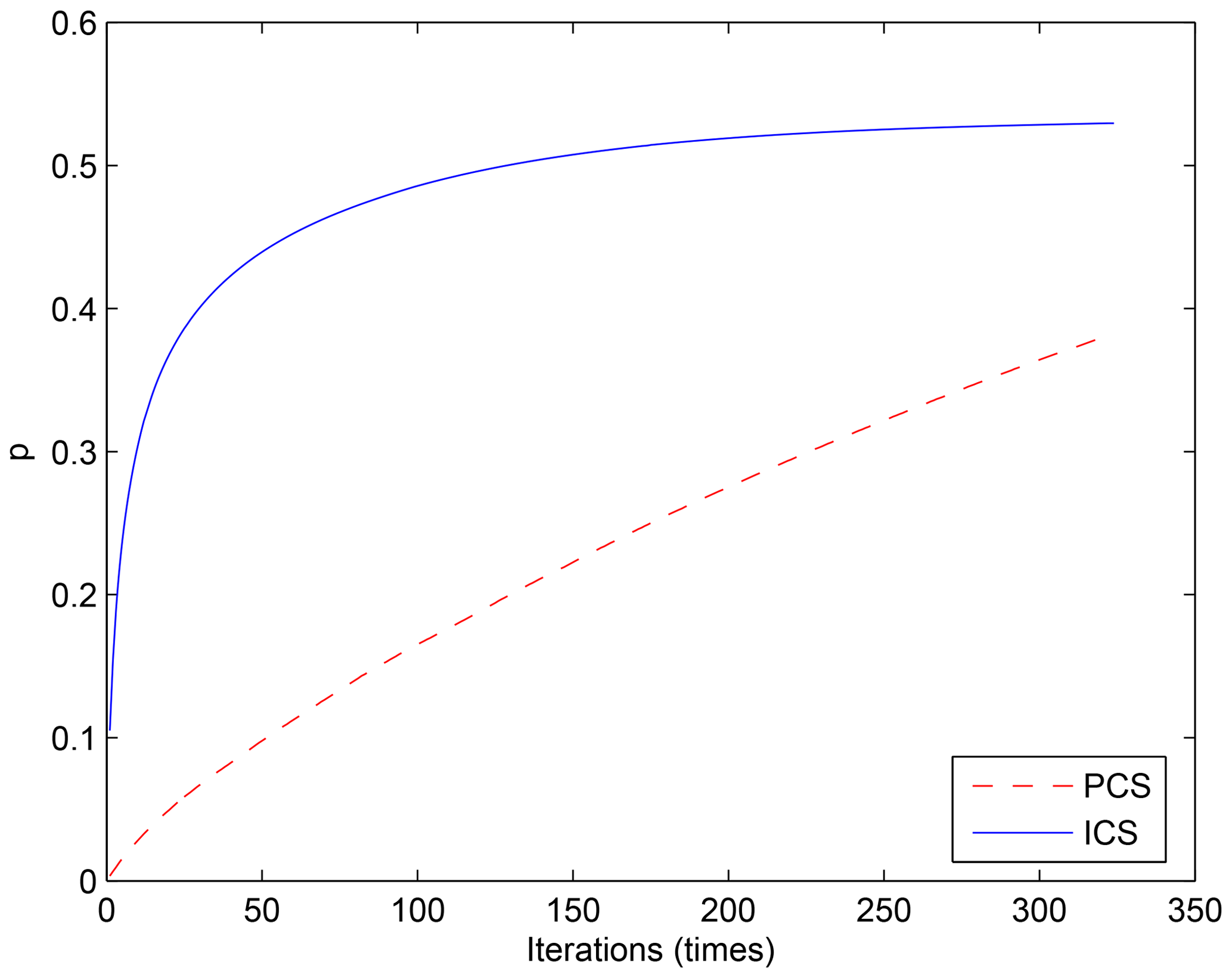
Figure 5 The relationship between the number of iterations and ARI. The blue line represents the result of ICS. The dashed red line stands for the result of PCS.

The ARI for PCS tends to be 0.38 and is not convergent, thus the PCS method needs to be improved. In this paper, the atmosphere is divided into 137 layers and, based on the information content and iteration, 324 channels are selected for each layer. Then, the temperature profile of each layer can be retrieved based on statistical inversion (see Sect. 4). The relationship between the number of iterations and the ARI for ICS is shown in Fig. 5b. When the number of iterations approaches 100, the ARI of ICS tends to be stable and reaches 0.54. Thus, in terms of the ARI and convergence, the ICS method is better than that of PCS.

Furthermore, because an iterative method is used to select channels, the order of each selected channel is determined by the contribution from the ARI. The weighting function matrix of the top 324 selected channels, according to channel order, is shown in Fig. 6.

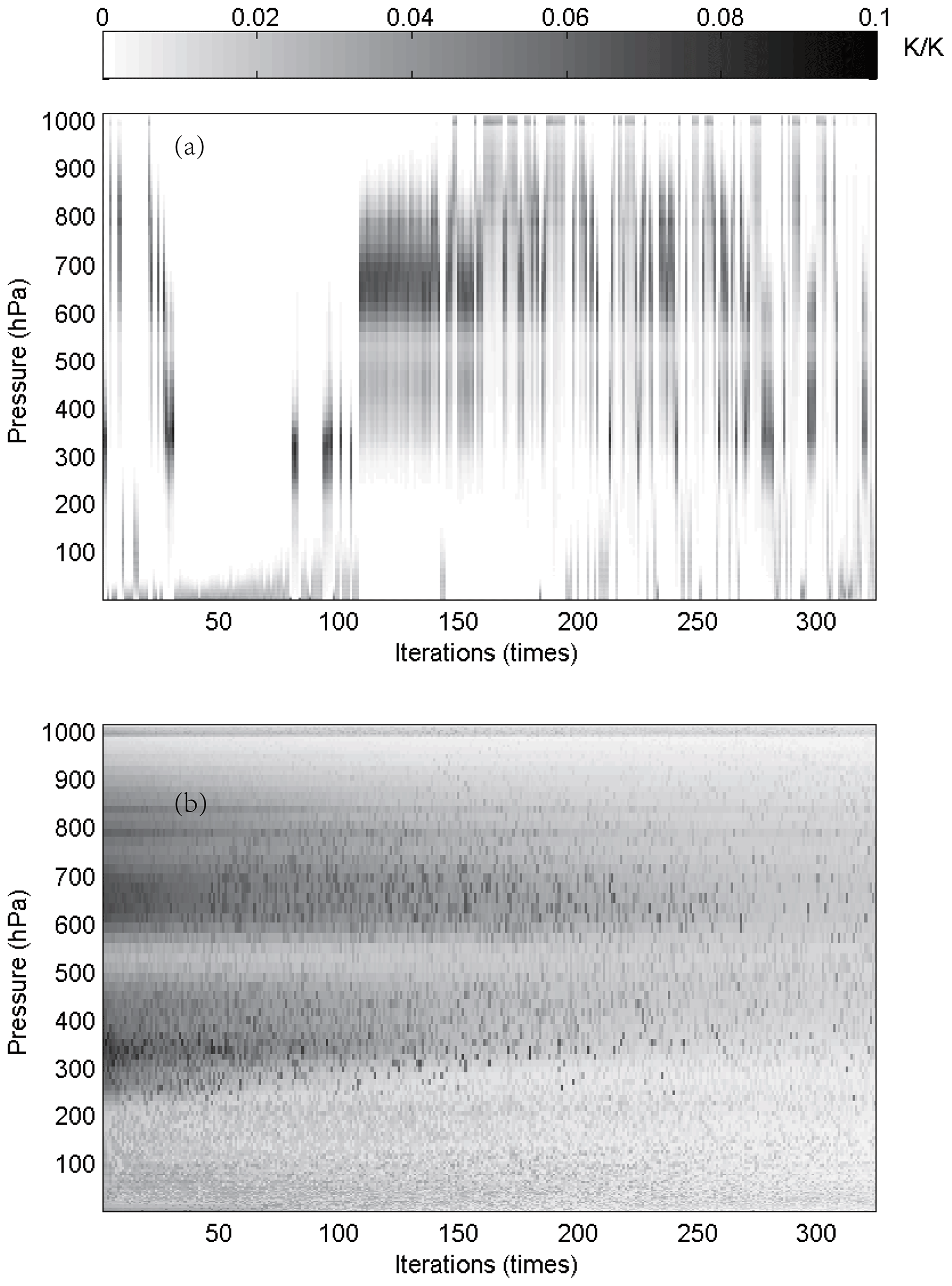
Figure 6 The relationship between the number of iterations and the weighting function of the top 324 selected channels (shaded): (a) ICS and (b) PCS.

As illustrated in Fig. 6, in the first 100 iterations, the distribution of the temperature weighting function for PCS is relatively scattered; it does not reflect continuity between the adjacent layers of the atmosphere. Besides, the ICS result is better than that of PCS, showing that (1) the distribution of the temperature weighting function is more continuous and reflects the continuity between adjacent layers of the atmosphere and (2) regardless of the number of iterations, the maximum value of the weighting function is stable near 300–400 and 600–700 hPa, without scattering, which is closer to the situation in real atmosphere.

4 Statistical multiple-regression experiment

4.1 Temperature profile database

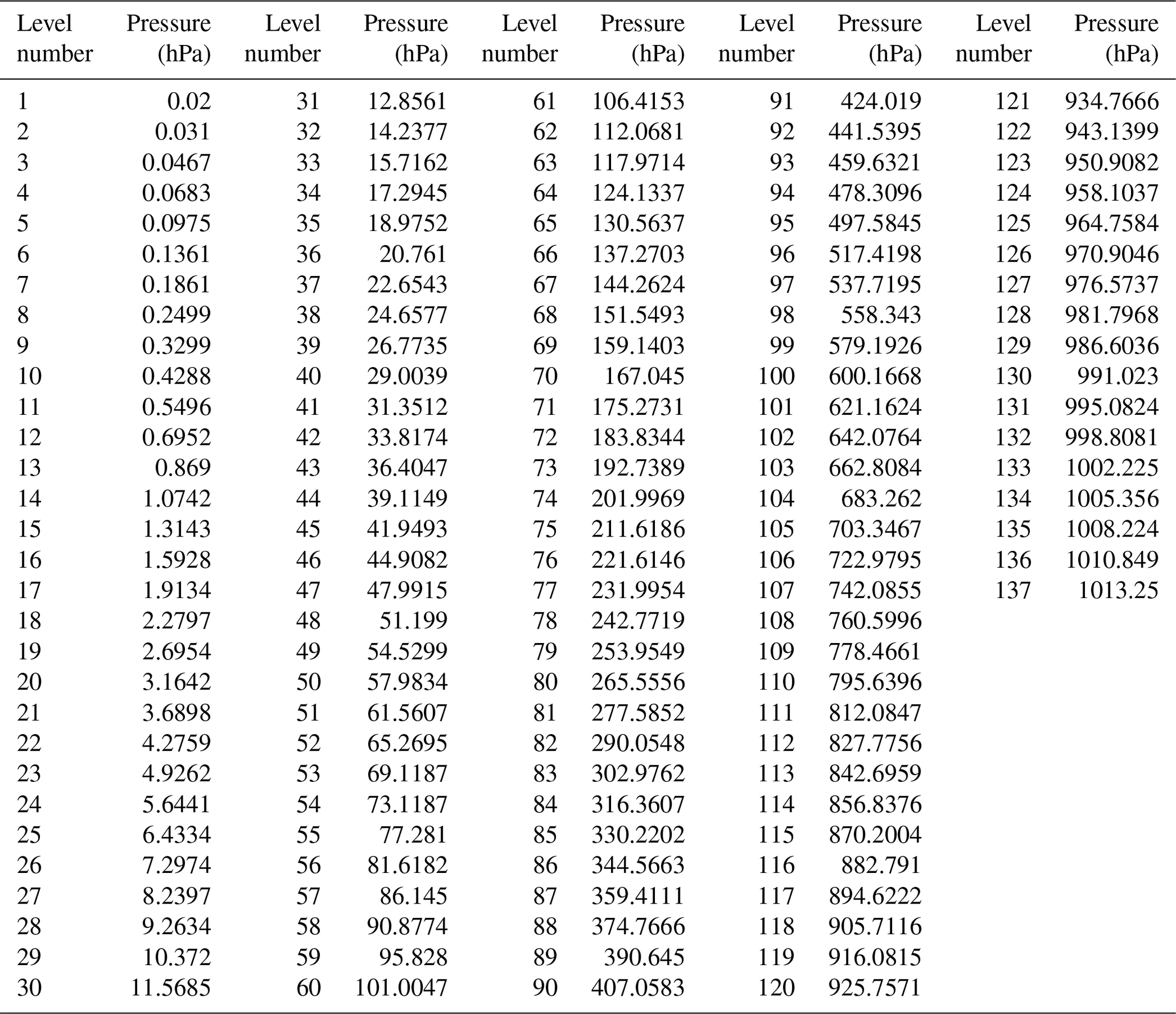
A new database including a representative collection of 25 000 atmospheric profiles from the European Centre for Medium-range Weather Forecasts (ECMWF) was used for the statistical inversion experiments. The profiles were given in a 137-level vertical grid extending from the surface up to 0.01 hPa. The database was divided into five subsets focusing on diverse sampling characteristics, such as temperature, specific humidity, ozone mixing ratio, cloud condensates and precipitation. In contrast with earlier releases of the ECMWF diverse profile database, the 137-level database places greater emphasis on preserving the statistical properties of sampled distributions produced by the Integrated Forecasting System (IFS) (Eresmaa and McNally, 2014; Brath et al., 2018). IFS-137 spans the period from 1 September 2013 to 31 August 2014. There are two operational analyses each day (at 00:00 and 12:00 Z), and approximately 13 000 atmospheric profiles over the ocean. The pressure levels adopted for IFS-137 are shown in Table A2 (see Table A2 in Appendix A).

The locations of selected profiles of temperature, specific humidity and cloud condensate subsets of the IFS-91 and IFS-137 databases are plotted on the map in Fig. 7. In the IFS-91 database, the sampling is fully determined by the selection algorithm, which makes the geographical distributions very inhomogeneous. Selected profiles represent those regions where gradients of the sampled variable are the strongest: in the case of temperature, midlatitudes and high latitudes dominate, while humidity and cloud condensate subsets concentrate at low latitudes. However, the IFS-137 database shows a much more homogeneous spatial distribution in all the sampling subsets, which is a consequence of the randomized selection.

Figure 7 Locations of selected profiles in the temperature (a, b), specific humidity (c, d) and cloud condensate (e, f) sampled from subsets of the IFS-91 (a, c, e) and IFS-137 (b, d, f) databases (from https://www.nwpsaf.eu/site/update-137-level-nwp-profile-dataset/, last access: 11 January 2020).

The temporal distribution of the selected profiles is illustrated in Fig. 8. The coverage of the IFS-137 dataset is more homogeneous than the IFS-91 dataset. Moreover, the IFS-137 database supports the mode with input parameters, such as detection angle, 2 m temperature and cloud information. Therefore, it is feasible to use the selected samples in a statistical multiple-regression experiment.

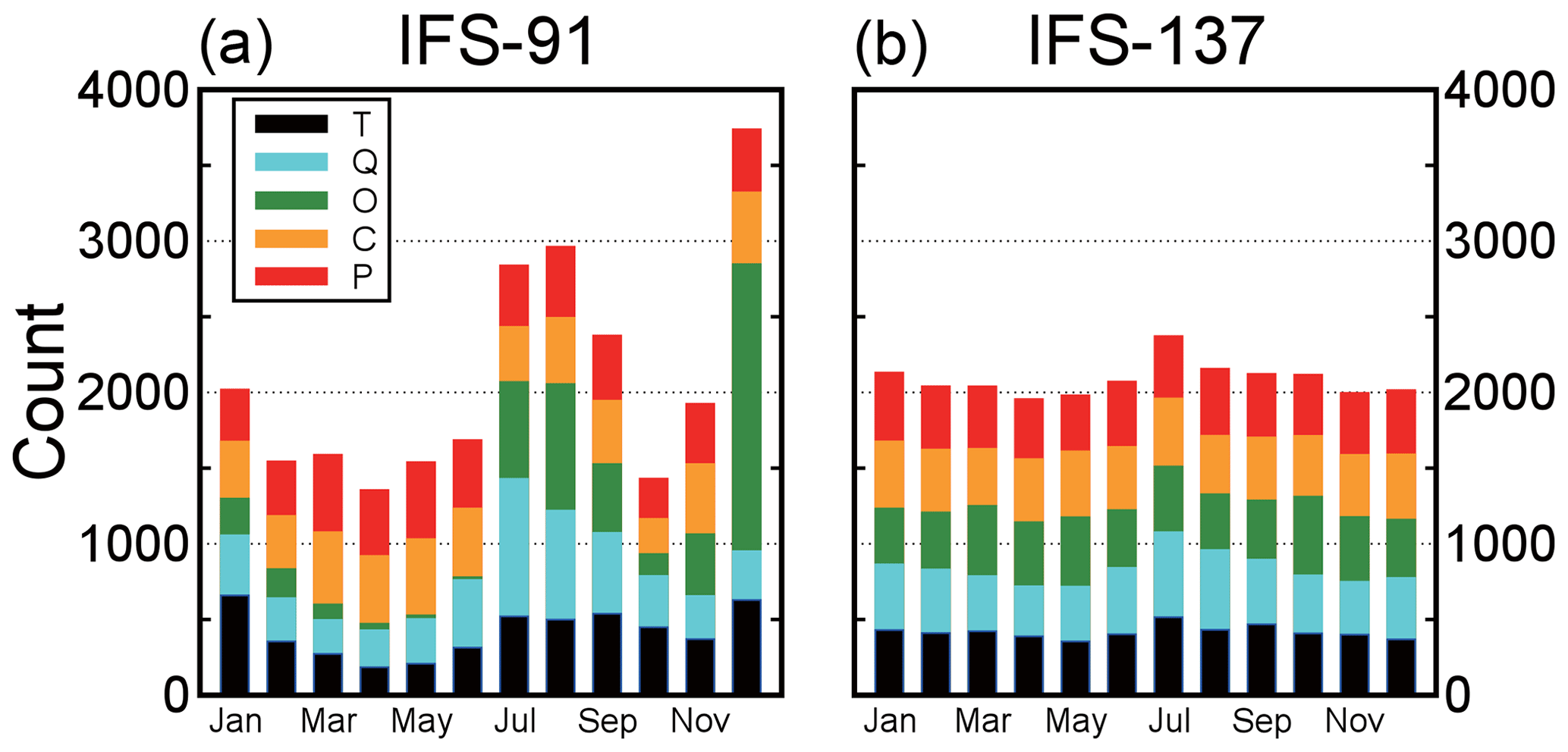
Figure 8 Distribution of profiles within the calendar months in IFS-91 (a) and IFS-137 (b) databases. Different subsets are shown in different colors. Black parts stand for temperature. Blue parts represent specific humidity. Green parts indicate ozone subset. Orange parts stand for cloud condensate. Red parts represent precipitation. Taken from https://www.nwpsaf.eu/site/update-137-level-nwp-profile-dataset/ (last access: 26 April 2019).

4.2 Experimental scheme

In order to verify the retrieval effectiveness of ICS, 5000 temperature profiles provided by the IFS-137 were used for statistical inversion comparison experiments. The steps are as follows.

• A total of 5000 profiles and their corresponding surface factors, including surface air pressure, surface temperature, 2 m temperature, 2 m specific humidity and 10 m wind speed, are put into the RTTOV mode. Then, the simulated AIRS spectra are obtained.

• The retrieval of temperature is carried out in accordance with Eq. (23). The 5000 profiles are divided into two groups. The first group of 2500 profiles is used to obtain the regression coefficient, and the second group of 2500 is used to test the result.

• The results are then verified; the test is carried out based on the standard deviation between the retrieval value and the true value.

4.3 Results and discussion

For the statistical inversion comparison experiments, the standard deviation of temperature retrieval is shown in Fig. 9. First, because PCS does not take channel sensitivity as a function of height into consideration, the retrieval result of PCS is inferior to that of ICS. Second, by comparing the results of ICS and NCS we found that below 100 hPa, since the method used in this paper considers near ground to be less of an influencing factor, the channel combination of ICS is slightly inferior to that of NCS, but the difference is small.

From 100 to 10 hPa, the retrieval temperature of ICS in this paper is consistent with that of NCS, slightly better than the channel selected for NCS. From 10 to 0.02 hPa, near the space layer, the retrieval temperature of ICS is better than that of NCS. In terms of the standard deviation, the channel combination of ICS is slightly better than that of PCS from 100 to 10 hPa. From 10 to 0.02 hPa, the standard deviation of ICS is lower than that of NCS by about 1 K, meaning that the retrieval result of ICS is better than that of NCS.

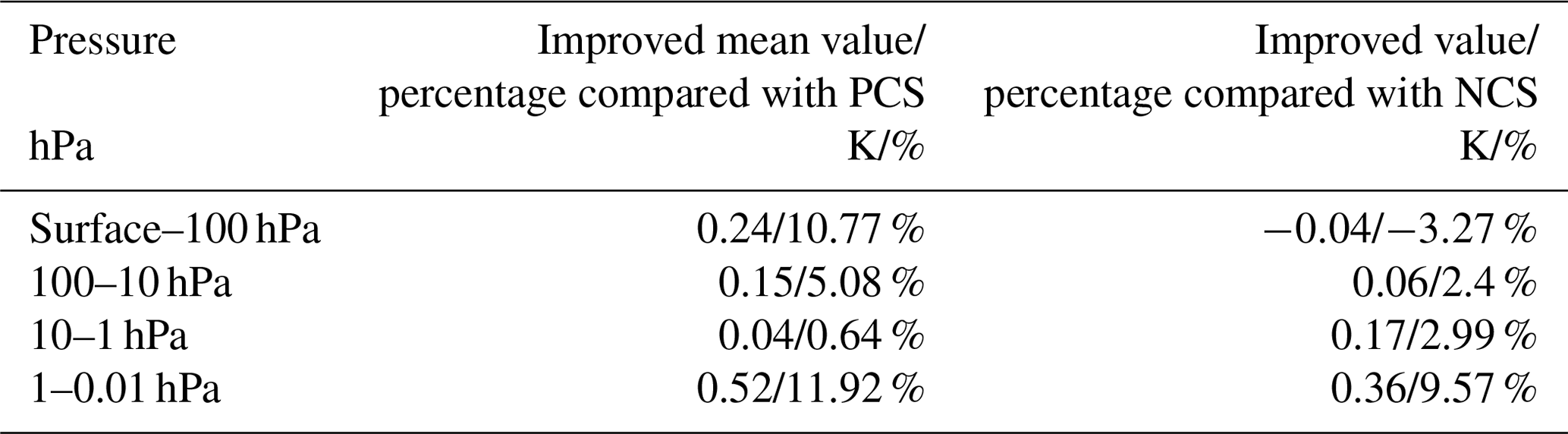
In order to further illustrate the effectiveness of ICS, the mean improvement value of the ICS and its percentages compared with the PCS and NCS at different heights are shown in Table 1. Because PCS does not take channel sensitivity as a function of height into consideration, the retrieval result of PCS is inferior to that of ICS. In general, the accuracy of the retrieval temperature of ICS is improved. Especially from 100 to 0.01 hPa, the mean value of ICS is evidently improved by more than 0.5 K, which means the accuracy can be improved by more than 11 %. By comparing the results of ICS and NCS we found that below 100 hPa, since the method used in this paper considers near ground to be less of an influencing factor, the channel combination of ICS is slightly inferior to that of NCS, but the difference is small. From 100 to 0.01 hPa, the mean value of ICS is improved by more than 0.36 K, which means the accuracy can be improved by more than 9.6 %.

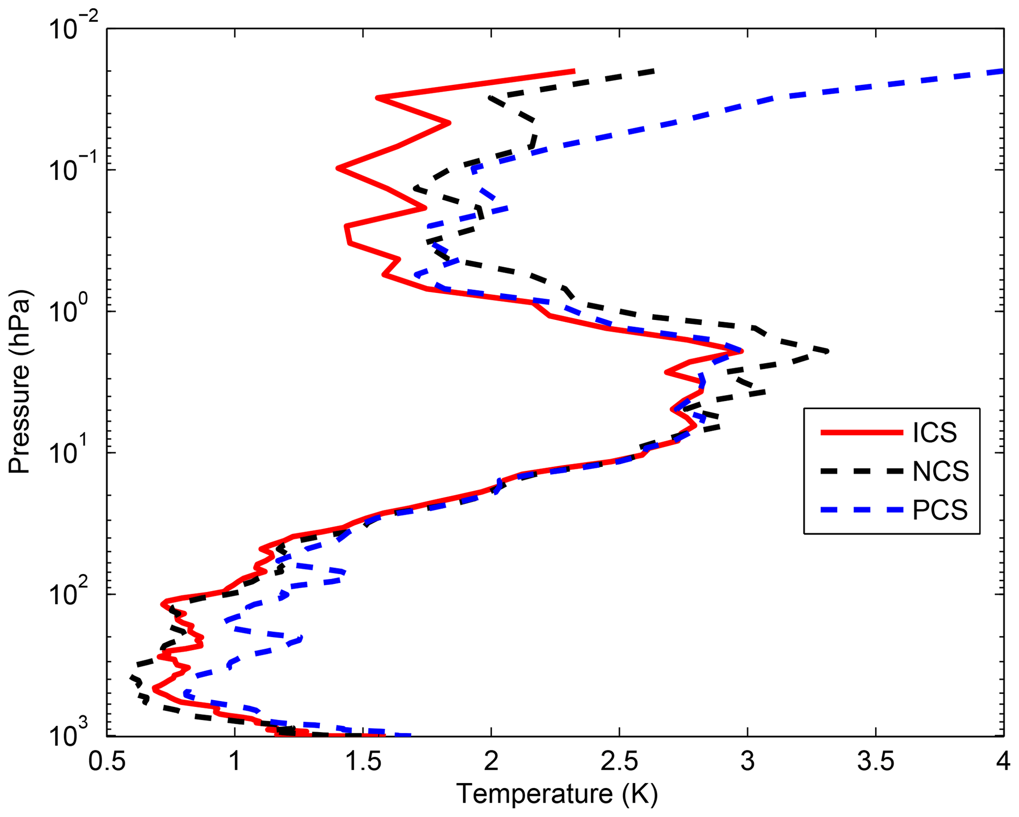
Figure 9 The temperature profile standard deviation of statistical inversion comparison experiments. The red line indicates the result of ICS. The dashed black line stands for the result of NCS. The dashed blue line represents the result of PCS.

Table 1 The mean improvement value of the ICS and its percentages compared with the PCS and NCS at different heights.

This is because, as shown in Fig. 4, (1) stratosphere and mesosphere is less affected by the ground surface, thus the retrieval result of PCS is better than that of NCS. (2) Due to the method selected in this paper, there are more channels at 4.2 µm for N₂O and 4.3 µm for CO₂ absorption bands, and the channel combination of PCS is superior to that of NCS for atmospheric temperature observation in the high-temperature zone. Moreover, ICS takes channel sensitivity as a function of height into consideration, thus its retrieval result is improved.

5 Statistical inversion comparison experiments in four typical regions

The accuracy of the retrieval temperature varies from place to place and changes with atmospheric conditions. Therefore, in order to further compare the inversion accuracy under different atmospheric conditions, this paper has divided the atmospheric profile from the IFS-137 database introduced in Sect. 4 into four regions: the equatorial zone, subtropical regions, midlatitude regions and the Arctic. The average temperature profiles in these four regions are shown in Fig. 10. The retrieval temperature varies from place to place and changes with atmospheric conditions. In order to further compare the regional differences of inversion accuracy, the temperature standard deviations of ICS in four typical regions are compared in Sect. 5.2.

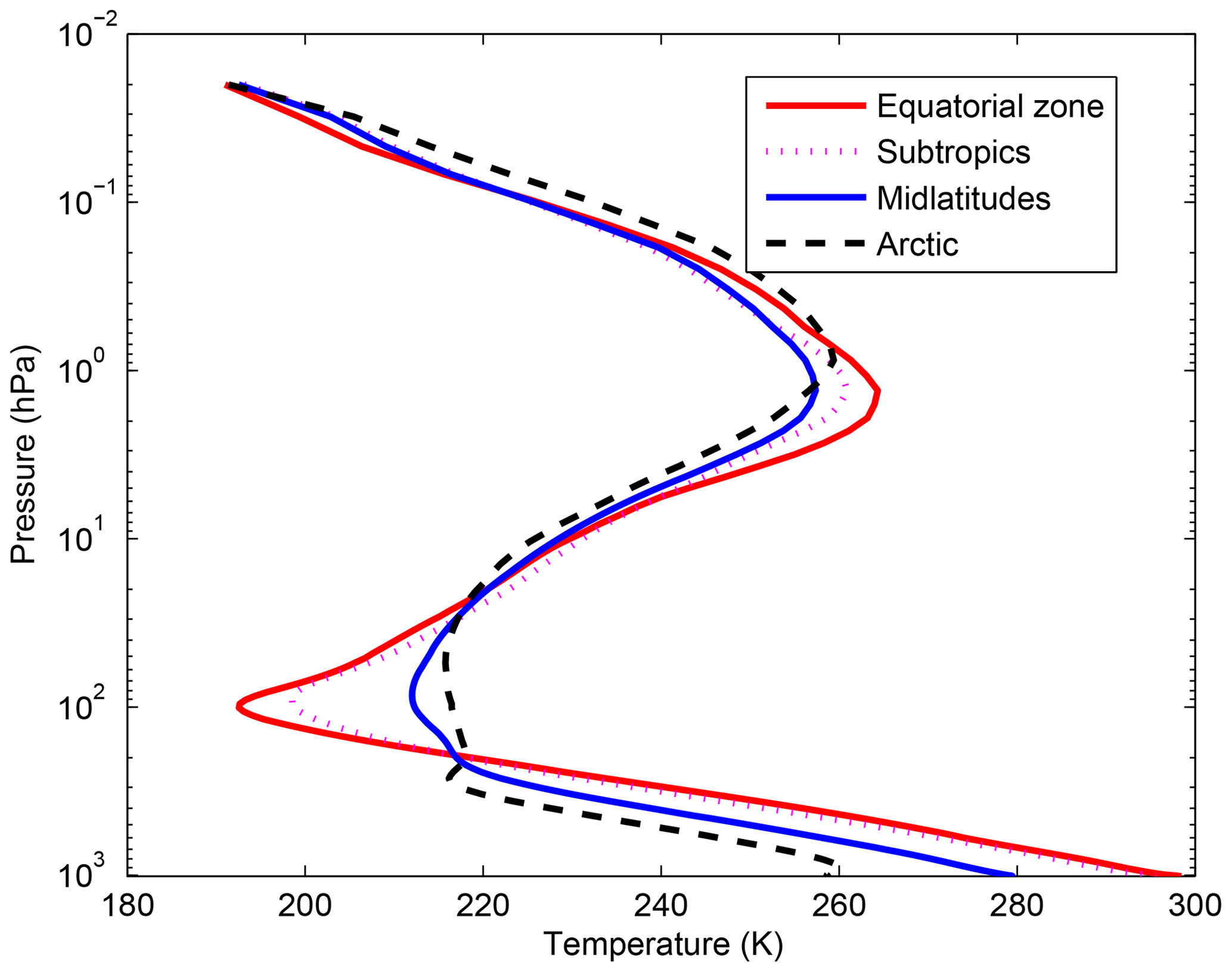
Figure 10 The average temperature profiles in four typical regions. The red line indicates the equatorial zone. The dashed pink line stands for the subtropics. The dashed blue line represents the midlatitude region. The dashed black line stands for the Arctic.

5.1 Experimental scheme

In order to further illustrate the different accuracy of the retrieval temperature using our improved channel selection method under different atmospheric conditions, the profiles in four typical regions were used for statistical inversion comparison experiments. The experimental steps are as follows:

• A total of 2500 profiles in Sect. 4 are used to work out the regression coefficient.

• The atmospheric profiles of the four typical regions, i.e., the equatorial zone, subtropical regions, midlatitude regions and the Arctic, are used for statistical inversion comparison experiments and to test the result.

• The results are then verified; the test is carried out based on the standard deviation between the retrieval value and the true value.

5.2 Results and discussion

Using statistical inversion comparison experiments in four typical regions, the standard deviation of temperature retrieval is shown in Fig. 11. Generally, the retrieval temperature by ICS is better than that of NCS and PCS. In particular, above 1 hPa (the stratosphere and mesosphere) the standard deviation of atmospheric temperature can be improved by 1 K with PCS and NCS. Thus, ICS shows a great improvement. The results were consistent with Sect. 4.

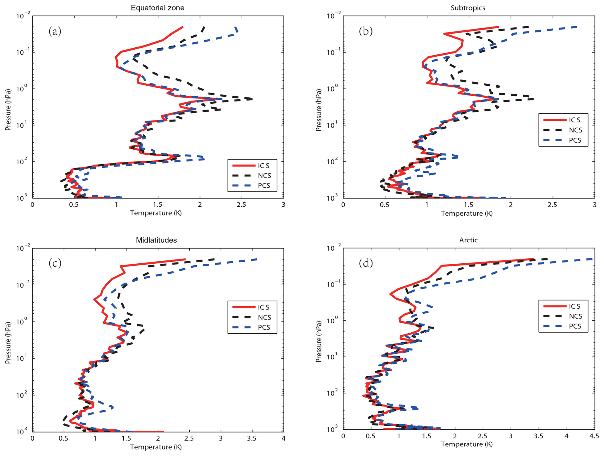
Figure 11 The temperature profile standard deviation of statistical inversion comparison experiments in four typical regions. The red line indicates the result of ICS. The dashed black line stands for the result of NCS. The dashed blue line represents the result of PCS. The panels show data for the following regions: (a) the equatorial zone, (b) subtropical regions, (c) midlatitude regions and (d) the Arctic.

In order to further compare the regional differences of inversion accuracy, the temperature standard deviation of ICS in four typical regions are compared in Fig. 12.

Figure 12 The temperature standard deviation of ICS in four typical regions. The red line indicates the result from the equatorial zone. The dashed pink line represents the result from the subtropics. The blue line represents the result from midlatitudes. The dashed black line stands for the result from the Arctic.

The temperature standard deviations of the ICS in the four typical regions are large (Fig. 12). Below 100 hPa, due to the high temperature in the equatorial zone, the channel combination of ICS is better than that of PCS and NCS for atmospheric temperature observation at higher temperature. The standard deviation is 0.5 K. Due to the method selected in this paper there are more channels at 4.2 µm for N₂O and 4.3 µm for CO₂ absorption bands, which has been previously described in Sect. 3. Near the tropopause, the standard deviation of the equatorial zone increases sharply. It is also due to the sharp drops in temperature. However, the standard deviation of the Arctic is still around 0.5 K. From 100 to 1 hPa, the standard deviation of ICS is 0.5 to 2 K. With the increase in latitude, the effectiveness considerably increases. According to Fig. 11, ICS takes channel sensitivity as a function of height into consideration, thus its retrieval result is better.

Although the improvements of ICS in the four typical regions are different, in general, the accuracy of the retrieval temperature of ICS is improved. Because PCS does not take channel sensitivity as a function of height into consideration, the retrieval result of PCS is inferior to that of ICS. In general, the accuracy of the retrieval temperature of ICS is improved.

6 Conclusions

In recent years, the atmospheric layer in the altitude range of about 20–100 km has been named “the near-space layer” by the aeronautical and astronautical communities. It is between the space-based satellite platform and the aerospace vehicle platform, which is the transition zone between aviation and aerospace. Its unique resource has attracted a lot of attention from many countries. Research and exploration, therefore, on and of the near-space layer are of great importance. A new channel selection scheme and method for hyperspectral atmospheric infrared sounder AIRS data based on layering is proposed. The retrieval results of ICS concerning the near-space atmosphere are particularly good. Thus, ICS aims to provide a new and an effective channel selection method for the study of the near-space atmosphere using the hyperspectral atmospheric infrared sounder.

An improved channel selection method is proposed, based on information content in this paper. A robust channel selection scheme and method are proposed, and a series of channel selection comparison experiments are conducted. The results are as follows.

• Since ICS takes channel sensitivity as a function of height into consideration, the ARI of PCS only tends to be 0.38 and is not convergent. However, as the 100th iteration is approached, the ARI of ICS tends to be stable, reaching 0.54, while the distribution of the temperature weighting function is more continuous and closer to that of the actual atmosphere. Thus, in terms of the ARI, convergence and the distribution of the temperature weighting function, ICS is better than PCS.

• Statistical inversion comparison experiments show that the retrieval temperature of ICS in this paper is consistent with that of NCS. In particular, from 10 to 0.02 hPa (the stratosphere and mesosphere), the retrieval temperature of ICS is obviously better than that of NCS at about 1 K. In general, the accuracy of the retrieval temperature of ICS is improved. Especially, from 100 to 0.01 hPa, the accuracy of ICS can be improved by more than 11 %. The reason is that stratosphere and mesosphere are less affected by the ground surface, thus the retrieval result of ICS is better than that of NCS. Additionally, due to the method selected in this paper, there are more channels at 4.2 µm for the N₂O and at 4.3 µm for the CO₂ absorption bands, and the channel combination of ICS is better than that of NCS for atmospheric temperature observation at higher temperature.

• Statistical inversion comparison experiments in four typical regions indicate that ICS in this paper is significantly better than NCS and PCS in different regions and shows latitudinal variations, which shows potential for future applications.

Appendix A

Table A1 Pressure levels adopted for RTTOV v12: 54 pressure level coefficients and profile limits within which the transmittance calculations are valid. Note that the gas units here are ppmv. (From https://www.nwpsaf.eu/site/software/rttov/ last access: 11 January 2020, RTTOV Users guide).

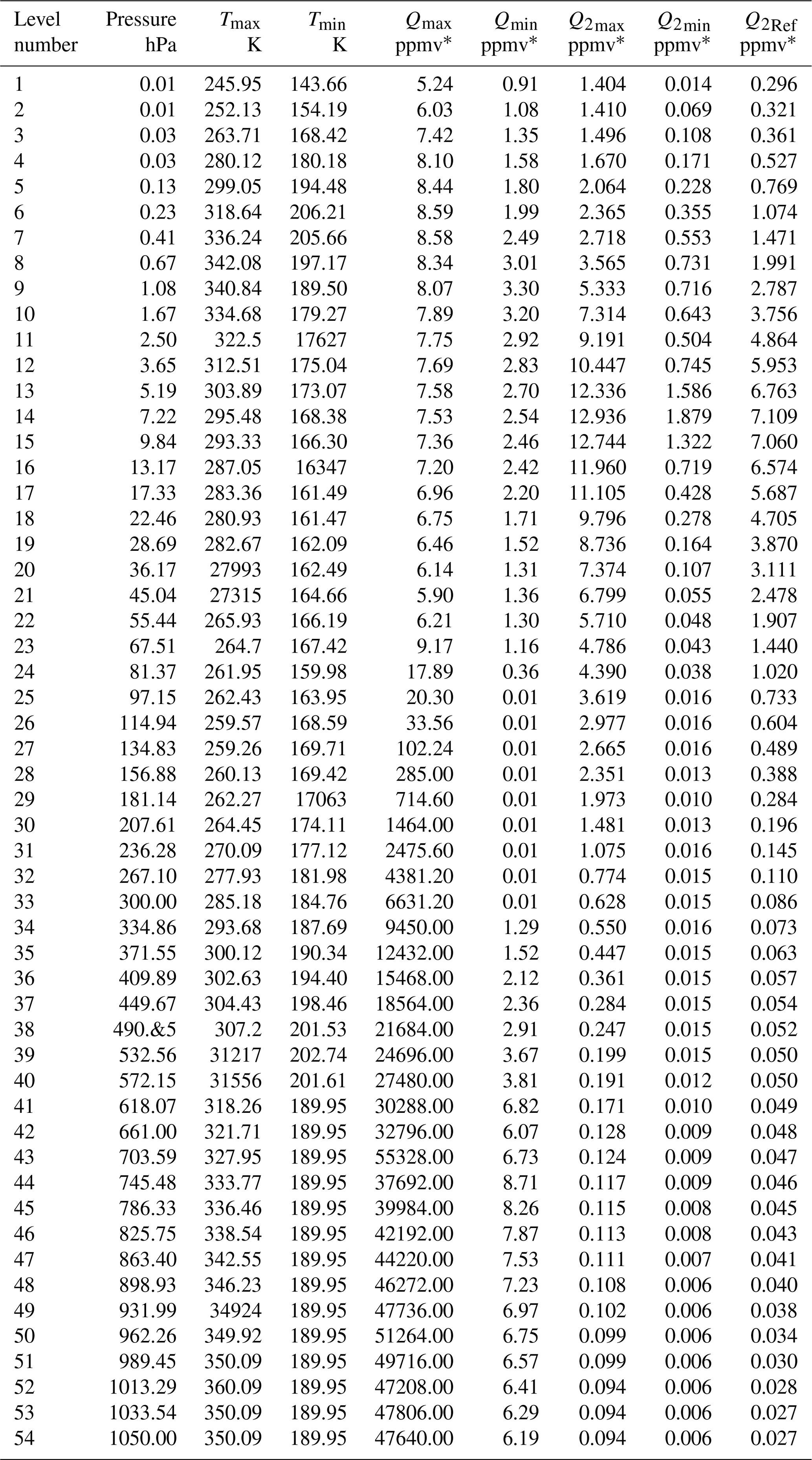
Table A2 Pressure levels adopted for IFS-137: 137 pressure levels (in hPa).