the Creative Commons Attribution 4.0 License.
the Creative Commons Attribution 4.0 License.
 | 27 Nov 2020
Three decades of tropospheric ozone lidar development at Garmisch-Partenkirchen, Germany
Thomas Trickl
Helmuth Giehl
Frank Neidl
Matthias Perfahl
Hannes Vogelmann
Since 1988 two ozone lidar systems have been developed at IMK-IFU (Garmisch-Partenkirchen, Germany). A stationary system, operated at the institute, has yielded about 5000 vertical profiles of ozone from next to the ground to typically 3 km above the tropopause and has contributed data for a large number of scientific investigations. A mobile system was successfully operated in a number of field campaigns after its completion in 1996, before it was destroyed in major flooding in May 1999. Both systems combine high data quality with high vertical resolution dynamically varied between 50 m in the lower troposphere and 250–500 m below the tropopause (stationary system). The stationary system has been gradually upgraded over the years. The noise level of the raw data has reached about of the input range of the transient digitizers after minor smoothing. As a consequence, uncertainties in the ozone mixing ratios of 1.5 to 4 ppb have been achieved up to about 5 km. The performance in the upper troposphere, based on the wavelength pair 292–313 nm, varies between 5 and 15 ppb depending on the absorption of the 292 nm radiation by ozone and the solar background. In summer it is therefore planned to extend the measurement time from 41 s to a few minutes in order to improve the performance to a level that will allow us to trust automatic data evaluation. As a result of the time needed for manual refinement the number of measurements per year has been restricted to under 600. For longer time series automatic data acquisition has been used.
- Article
(5993 KB) - Full-text XML
- BibTeX
- EndNote


Lidar measurements of tropospheric ozone have resulted in important contributions to atmospheric research. Large variations of the concentrations on timescales of less than 1 h may be observed, which have led to insight into a number of tropospheric transport processes (see Table A1 for a large number of examples). In addition, measurements with ozone lidar systems have contributed to numerous air-quality studies (Table A2). Due to considerable technical progress, rather small changes in the volume mixing ratio of just a few parts per billion (ppb) can currently be resolved, which is necessary for also distinguishing the influence of minor contributions and for reliable trend studies.
Still, important tasks in tropospheric ozone research exist, such as a clarification of the positive ozone trend observed until 2003 at high-altitude observational sites in Europe (Scheel, 2003; Ordoñez et al., 2007) despite the pronounced reduction of ozone precursors over Europe (Jonson et al., 2006; Vautard et al., 2006), a detailed analysis of the rather complex contributions of different sources to long-range transport, and the influence of vertical mixing on free-tropospheric layers, in particular on stratospheric air intrusions (Trickl et al., 2014, 2015, 2016). Although vertical sounding, including lidar measurements of complementary quantities such as aerosols and water vapour (e.g. Trickl et al., 2014, 2015, 2020; Strawbridge et al., 2018; Fix et al., 2019), can yield key information for the understanding of the role of the underlying atmospheric processes, for a long time there was no significant growth in the number of tropospheric ozone lidar stations towards something like an international network. By contrast, more and more ozone lidar systems have even been shut down. Opposite to this development, the Tropospheric Ozone Lidar Network (TOLNet, https://www-air.larc.nasa.gov/missions/ TOLNet/, last access: 19 November 2020) with seven lidar stations was recently established in North America (e.g. Newchurch et al., 2016; Wang et al., 2017; Leblanc et al., 2018). It is important to note that even vertical profiles from the impressive MOZAIC (Measurements of Ozone and Water Vapor by Airbus In-Service Aircraft) (Marenco et al., 1998) database are not able to resolve the fine-scale temporal variability of the vertical distribution of trace constituents because of the rather confined time slots for aircraft departures and arrivals at the individual airports. Satellite measurements cannot yield the necessary information because of presently insufficient spatial resolution and global coverage within a day.
With a few exceptions, mostly ultraviolet (UV) differential-absorption lidar (DIAL) systems for tropospheric applications have been proposed and developed since 1975 (Papayannis et al., 1990; Table A3). Here, the advantages of high Rayleigh backscattering and strong absorption cross sections are combined. In Europe, the TESLAS (Tropospheric Environmental Studies by Laser Sounding) subproject of EUROTRAC (EUREKA Project on Transport and Chemical Transformation of Environmentally Relevant Trace Constituents in the Troposphere over Europe; EUROTRAC, 1997) has resulted in the coordinated development of several state-of-the art ozone lidar systems (TESLAS, 1997). Lidar sounding of tropospheric ozone is a demanding technical task (Weitkamp et al., 2000) because of the considerable dynamical range of the backscatter signal covering up to about 8 decades, the presence of aerosols and clouds, interfering trace gases such as SO2 and NO2, and the solar background (stratospheric ozone measurements are normally made during night-time), all necessitating an elaborate optical and electronic design. The data evaluation is based on derivative formation that is particularly sensitive to signal perturbations that set limitations to resolving the frequently rather small changes in free-tropospheric ozone.
At IFU (Fraunhofer-Institut für Atmosphärische Umweltforschung; now Karlsruher Institut für Technologie, IMK-IFU), a differential-absorption lidar (DIAL) with a particularly wide operating range from next to the ground to the upper troposphere was completed in 1990 in the framework of TESLAS and subsequently applied for a full year (1991) within the TOR (Tropospheric Ozone Research; Kley et al., 1997) subproject of EUROTRAC (Carnuth et al., 2002). The operating range of this system was extended to roughly 15 km by introducing three-wavelength operation (Eisele and Trickl, 1997). Due to thorough upgrading of the data acquisition system an uncertainty level of 1.5 to 4 ppb has been achieved up to the mid-troposphere (slightly higher in the upper free troposphere, depending on the ozone concentration and solar background).
In the mid-1990s a mobile ozone DIAL was additionally built in cooperation with OHB System (Bremen, Germany; Brenner et al., 1997). This system, which was completed in spring 1996 and exhibited at the 1996 International Laser Radar Conference, could be operated in a vertical range between 0.2 and more than 4 km with a similar accuracy as our stationary system at low altitudes. It was used in a number of field campaigns before it was destroyed by 2 m of water during major flooding in southern Bavaria in May 1999 while waiting for the VOTALP Munich field campaign (VOTALP II, 2000).
In this paper we review the experience gained with these two lidar systems. The development of these two systems has significantly contributed to the state of the art in this field. Meanwhile, even the dream of meaningful automatic data evaluation looks feasible due to the technical progress made. Most approaches and instruments used are the same in both lidar systems, which simplifies the description.
Most of the paper is devoted to the stationary DIAL. We describe only deviating design properties of the much compacter mobile system such as the laser approach and the wavelength separation technique chosen. This system has been extensively used over 3 decades, but no full-size technical description has been given. We do not want to give a full description of all the technical improvements made over the years. Just the decisive steps are reported.
Most of the approaches of the ozone DIAL systems have also been successfully transferred to the other lidar systems of IMK-IFU.
In both IFU DIAL systems, fixed-frequency lasers and stimulated Raman shifting in H2 and D2 have been used for generating suitable “on” and “off” wavelengths (see de Schoulepnikov et al., 1997; Milton et al., 1998, for general overviews). In this way just a single high-power laser source is needed. Both systems are three-wavelength lidars with two on wavelengths and one off wavelength. This offers the opportunity for wide-range operation starting below 0.3 km above the ground, with stronger absorption and accuracy as well as good vertical resolution for the shorter of the two on wavelengths and a range extension with lower vertical resolution for the longer on wavelength. In addition, the comparison of ozone profiles obtained from two separate wavelength pairs allows for internal quality control. In fact, as described in Sect. 6, for an optimum alignment and sufficient backscatter signal the agreement between the different ozone profiles is almost perfect. Apart from the wavelength separation methods, the basic optical layout principles and detection electronics are mostly the same. Both systems feature automatic data acquisition.
The stationary system (Fig. 1) is operated in two separate, rather large laboratories at IFU (47.477∘ N, 11.064∘ E; 740 m a.s.l.). This offers several advantages such as a simple optical layout, good alignment control due to long beam paths, reduced thermal drifts because of no direct exposure of the laser system to outside air, and the long distance between detection electronics and the interfering laser system. Two separate power systems are used for the laser and electronics. The laser PC is connected to the cleaner power system for the electronics and controls the laser system via optical fibres. Remote control of the laser is achieved via RS232.
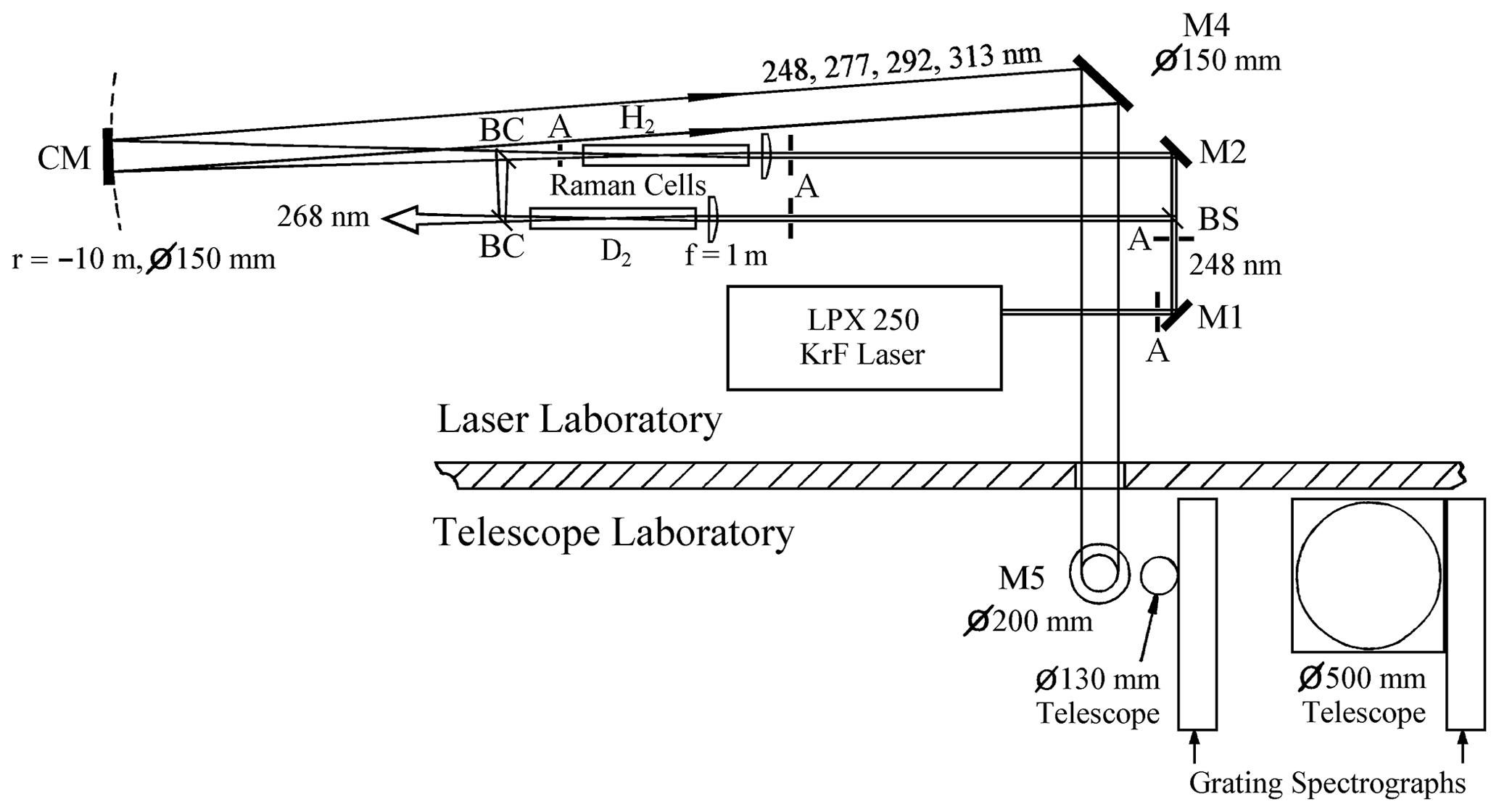
Figure 1Overview of the IFU stationary ozone DIAL system; the system covers two separate laboratories for the laser and the telescopes. Abbreviations are as follows. M1, M2: dielectric high-reflecting mirrors for 248 nm; SM: spherical mirror (M3), high-reflecting for 248 to 313 nm, f=5 m; M4, M5: dielectric mirrors, high-reflecting for 248 to 313 nm; BS: 50 % beam splitter; BC: wavelength-selective beam combiner, reflecting 99 % at 292 nm for an incidence angle of 45∘ and transmitting all the other lidar wavelengths with losses not exceeding 12 %. A: rectangular sand-blasted aluminium apertures for blocking divergent parts of the amplifier emission that would otherwise hit and evaporate the black surfaces of the optics holders, leading to more rapid ageing of the optics.
Due to the clean-air conditions prevailing at this rural site the wavelength choice is less critical. The ambient concentrations of SO2 and NO2, species with absorption bands in the spectral range of ozone DIAL systems, are low, which is known from the local long-term monitoring stations. Thus, the choice of the laser source was determined by high power in order to achieve a short measurement time. Krypton fluoride lasers have been used (Kempfer et al., 1994; Eisele and Trickl, 1997); since 1994 this has been a model with a maximum available average power of 54 W at 248.5 nm (all wavelengths in this paper are given for vacuum).
The laser choice was different for the mobile system (Fig. 2). A frequency-quadrupled Nd:YAG laser with up to 4.2 W of average power at 266.1 nm served as the basic source of ultraviolet (UV) light. This approach was preferred for several reasons: due to the expected operation in heavily polluted areas at least one wavelength combination (266–299 nm) reduces the cross-sensitivity with respect to SO2 and NO2 to about 0.01 ppb of ozone per part per billion of these species. Under such conditions, the perspective of low interference by aerosols is also important, which is fulfilled for short on wavelengths (Völger et al., 1996; Eisele and Trickl, 2005). Thus, wavelength combinations involving 266 nm are favourable. Finally, due to the choice of a solid-state laser source the dangerous gas handling in an excimer laser could be avoided, an issue for the mobile operation.
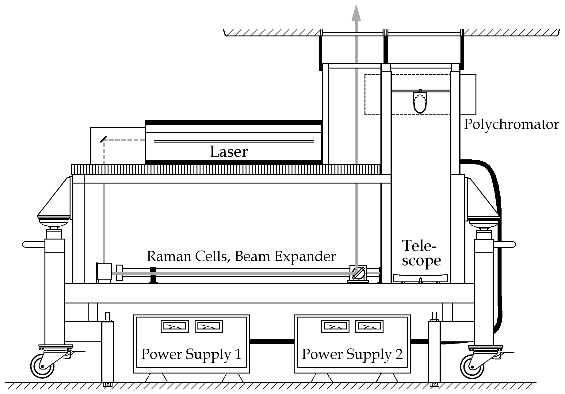
Figure 2Overview of the mobile ozone DIAL: the laser and the Raman-shifting components were mounted on optical tables at two different levels of a shock-isolated frame. The Newtonian telescope was located in a separate tower, with the secondary mirror directing the beam into a polychromator perpendicularly to the plane formed by the telescope and the outgoing laser beam. The covers of the Raman compartment (jalousies on both sides) and the telescope (door) were removed in this simple view. The laser power supply was delivered in two units custom-made to fit under the lower laser table. The entire frame was rolled into the lorry through the rear doors.
A clear design goal for the mobile system was a vertical range significantly exceeding the boundary layer by a few kilometres. This requirement was seen as crucial for meaningful investigations during air pollution field campaigns. The mobile ozone DIAL was mounted inside an air-conditioned truck (Fig. 2) and was designed for autonomous operation with an on-board power generator, batteries, automatic positioning (GPS), and detailed safety control management including rain and wind sensors, shutter control of the laser, and many interlocks. Critical safety conditions immediately overrode any other action. The operator could be automatically informed about incidents during night-time via telephone. After rain, the system could be restarted automatically, unless the laser was shut down (see Sect. 3.2).
The detection system of this DIAL was much simpler, with a less demanding optical set-up (single telescope for both near- and far-field detection, simple filter polychromator) and with fewer electronic components due to a sequential emission of two of the three operating wavelengths. All this resulted in a considerable reduction of costs, which at that time was an attractive perspective in view of the goal of our industrial partner of an affordable commercial system.
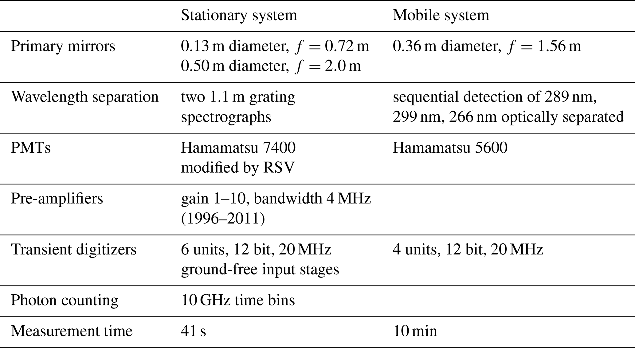
Overall specifications of the two systems are listed in Tables 1 and 2. All optical components and dielectric coatings have been provided by Laseroptik GmbH (Garbsen, Germany) unless otherwise specified.
Table 1Transmitter details (the numbers are given for normal operating conditions).
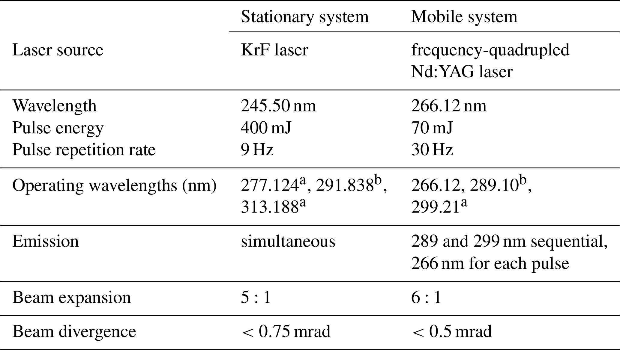
a Q1 line of first Stokes shift in H2 (Bragg et al., 1982; Dickensen et al., 2013): 4155.2521 cm−1. b Q2 second Stokes shift in D2 (Jennings et al., 1986): 2987.289 cm−1.
3.1 Stationary lidar
The transmitter of the system (Fig. 1, Table 1) is based on a KrF excimer laser (Lambda Physik, LPX 250, maximum repetition rate 100 Hz) consisting of a tunable narrowband oscillator and a three-pass power amplifier. CaF2 is used for transmitted optics. CaF2 is not birefringent, and thus polarization effects (Kempfer et al., 1994) and ageing are avoided. The energy was considerably enhanced by anti-reflection (AR) coating on the outer side windows of the amplifier gas cell and the beam splitter in front of the energy monitor. A pulse energy of up to 540 mJ was measured several metres away from the laser where divergent components also emerging from the amplifier can be separated and blocked by an aperture. For the lidar measurements the laser energy is usually set to 400 mJ. The unstable cavity of the amplifier yields a highly collimated rectangular beam with a divergence of 0.2 mrad. The wavelength was set for maximum output and the prism-grating combination never touched again. In 2010 measurements with a HighFinesse WS6 (Δλ=0.6 pm) wavelength meter carried out over several days yielded 248.5078 nm ± 0.0060 nm, in agreement with the results of Kempfer et al. (1994). The spectral bandwidth is specified as 0.2 cm−1 (6 GHz). Locking the amplifier to the oscillator can be nicely verified by an enhancement of the pulse energy by up to 70 mJ under our standard operating conditions.
The output of the KrF laser is split by a 50 % beam splitter and focused into two Raman cells with f=1.0 m AR-coated plano-convex CaF2 lenses. One cell is filled with hydrogen and the other one with deuterium, and the same pulse energy per cell as previously used for a single cell (Kempfer et al., 1994) is ensured (almost 0.2 J). A total of six Stokes components are generated in hydrogen, just 277.124 nm (S1) and 313.188 nm (S2) are taken (Table 1). For deuterium the second Stokes (S2) component (291.838 nm) is used. The outer surfaces of the CaF2 windows of the Raman cells are AR-coated. The inner ones are not coated because of the possibility of ageing in the presence of photolysed hydrogen. The pump radiation leaving the evacuated Raman cells is of the order of 160 mJ. The output of the Raman cells is combined with a pair of dichroic beam combiners and collimated with an f=5 m, 150 mm diameter concave spherical mirror. The beam combiners reflect 99 % of the 292 m radiation at 45∘ and transmit 88 to 90 % of all the other relevant spectral components. Overlap and pointing of the 292 nm beam are optimized by placing a wire cross in front of the D2 cell or behind the second beam combiner by watching the images of the cross in front of mirror M4.
The Raman conversion efficiency obtained with the LPX 250 laser system is lower than that previously published (Kempfer et al., 1994). We ascribe this to the smoother energy distribution in the beam profile of the new laser. As an example, Fig. 3 shows the conversion efficiencies obtained for hydrogen for a laser pulse energy of almost 200 mJ per Raman cell, attenuated by the optics, in particular by the single-side AR-coated cell entrance windows. The sum of all conversion efficiencies is less than 1.0 starting at already low pressures. This loss of overall energy is tentatively ascribed to optical breakdown. Above 3 bar the loss starts to level off. The non-negligible fourth Stokes emission (Kempfer et al., 1994) was not determined. The maximum second Stokes conversion efficiency for deuterium is approximately 17 % (at 11 bar). The operating pressures have been chosen at around 3.3 and 11 bar for H2 and D2, respectively.
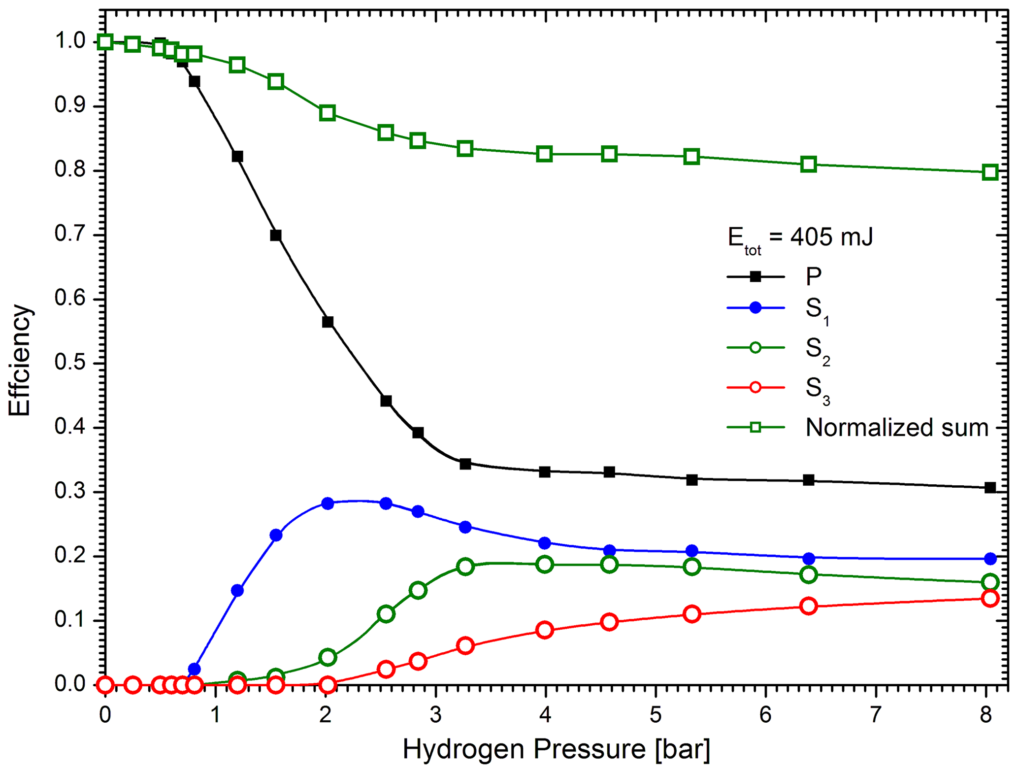
Figure 3Raman conversion efficiency (f=1.0 m) as a function of pressure for shifting the 248.5 nm radiation in hydrogen; the top curve (dark green) represents the sum of the residual pump energy and the first three Stokes emissions normalized to the pump energy at zero pressure. The less important higher Stokes emissions were not measured here but may contribute above 4 bar, which would shift the sum to higher values.
The conversion efficiency was determined for a laser repetition rate of 10 Hz in order to avoid damage to the power meter used. During the lidar measurements it turned out that the second Stokes output may increase when selecting a repetition rate of 100 Hz, sometimes even leading to range signal overflow in the transient digitizer. This effect was unexpected and must be taken into account when setting the detector supply voltages. We did not analyse this behaviour in detail.
Linear polarization is important for single-line output of the Raman shifters (Kempfer et al., 1994). Thus, we placed a Glan prism and a Fresnel rhomb (both from Halle) in the beam between the oscillator and amplifier. All mirrors and beam splitters of the transmitter section were manufactured with minimum polarization sensitivity. The Fresnel rhomb is rotated for optimum backscatter signal (Fig. 4). The strong modulation of the lidar signal in Fig. 4 is mainly caused by the holographic gratings used in the receivers (Sect. 3).
Due to the high average power of the laser system the time for a single ozone measurement, carried out with a repetition rate of 99 Hz, is as short as 41 s.
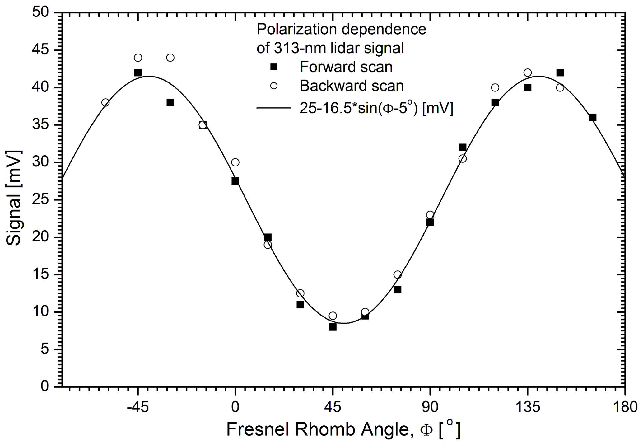
Figure 4313 nm backscatter signal as a function of the angle of the Fresnel rhomb (i.e. half the polarization angle): the strongest signal is achieved with the polarization of the radiation emitted into the atmosphere perpendicular to the grooves of the grating.
3.2 Mobile lidar
The pump laser of the mobile DIAL was a frequency-quadrupled Nd:YAG laser with a 30 Hz repetition rate and pulse energies of up to 140 mJ at 266 nm (Continuum, Powerlite 9030). The laser was selected because of a remote control option. The manufacturer promised external control of warm-up and rotation of the frequency doubling and quadrupling crystals. The 1064 and 266 nm powers were measured by two Molectron power meters for a PC-based power optimization. However, the computer control never worked properly: automatic warm-up of the laser was never achieved. The reason was a conflict with “keep-alive” pulses that had to be sent by the external control.
The quadrupling was achieved by using BBO (beta barium borate). This approach yielded high conversion efficiency and moderate thermal loading. However, after more than 1 year of infrequent operation of the lidar the surface of the crystal started to degenerate. This turbid layer did not strongly reduce the UV emission and polishing was therefore postponed.
At maximum pump energy (1.6 J at 1064 nm) the 266 nm radiation exhibited a ring-shaped mode at a pulse-energy level of 140 mJ. We reduced the pulse energy to 1.1 J. Still, 120 mJ could be produced, now with a filled beam profile. However, a hot spot formed that focused in the Raman-shifting compartment and we reduced the UV output to about 70 mJ for safety reasons. This hot-spot problem was solved by the manufacturer in a later (“precision”) version of the laser.
A ceramics shutter was added to the exit holes of the Powerlite laser that was controlled by both the safety system and the lidar PC. Closing the shutter was preferred to switching off the laser oscillator in order to maintain stable thermal conditions in the laser during an interruption.
A side view of the lidar including the entire transmitter is given in Fig. 2, which is the lower level of the frame in Fig. 5. Figure 5 shows the Raman-shifting compartment that also contained a 6:1 beam expander used for reducing the beam divergence. Rotating beam splitters were used for directing the laser pulses into the H2 and D2 cells. These beam splitters were based on circular quartz plates differently coated on the two halves of the surface: high-reflecting for the lidar wavelengths on one half and high-transmitting on the other one. The rotation was synchronized to the laser pulses. The control unit issued pulses for identifying the Raman cell actually passed for the data acquisition system. Two precision motors with measured out-of-axis rotation of just about ±2 and ±40 µrad, respectively, were chosen (KaVo, model EWL 4025; with custom-made electronic control).

Figure 5Lower compartment of the transmitter section of the mobile DIAL; the 266 nm beam enters vertically from the top compartment and hits the first of the two M1 mirrors. The polychromator is located above the two compartments as indicated by the broken line. Abbreviations are as follows. M1: high-reflecting mirror for 266 nm; M2: high-reflecting mirror for at least 266–300 nm; Ch: rotating beam splitter (“chopper”); L: f=1.00 m, AR-coated; M3: curved mirror, m, HR-coated for at least 266–300 nm; M4: curved mirror, m, coated for at least 266–300 nm; M5: rectangular mirrors, high-reflecting mirror for at least 266–300 nm; R1, R2: motorized rotation stages, mounted vertically and horizontally, respectively.
Due to high thermal sensitivity the emission wavelengths of Nd:YAG lasers may vary considerably from model to model. We derive a guess of the unknown pump wavelength of our Powerlite laser model from Trickl et al. (1989; 2007) and wavelength measurements for three other injection-seeded Nd:YAG lasers in our laboratory. The average pump wavelength is 266.120 nm ± 0.011 nm. This yields first-Stokes-shifted wavelengths of 289.103 nm (in D2) and 299.209 nm (in H2).
By focusing the 266 nm beam with an f=1.0 m plano-convex lens we reached maximum first Stokes (S1) conversion efficiencies of almost 50 % in both hydrogen and deuterium at pressures as low as 0.9 and 1.6 bar, respectively. This is remarkable in two respects: the theoretical Raman conversion efficiency reaches 50 % at higher pressures and the Raman gain of deuterium is substantially smaller than that of hydrogen (de Schoulepnikov et al., 1997). A total of 5 Stokes orders and 1 anti-Stokes order were visually observed for hydrogen, with fewer orders for deuterium. There was some contribution of the second Stokes order (particularly low at 1 bar due to gain competition with S1), but those for the higher orders were below the 1 mW detection threshold of the power meter used. Starting at pressures below the threshold for Raman conversion absorption was realized and, in H2, the conversion efficiency rapidly dropped to zero above about 1 bar. The same effect was also observed in pure helium and argon. Thus, we ascribe these observations to laser-induced breakdown. The role of the hot spot in igniting this breakdown could not be examined. Quite obviously, the Stokes emission was emitted prior to the breakdown maximum (see also Trickl, 2010a). In any case, the high conversion efficiency achieved was more than enough for the lidar operation.
Motivated by the hot-spot problem the focusing lens was replaced by a pair of crossed f=1.0 m cylindrical lenses during the final phase of operation of this lidar system. As suggested by Perrone and Piccinno (1997) this may result in a softer focus, a larger focal volume, and higher Raman conversion. The maximum possible distance between the two lenses was about 12 cm and was chosen for the lidar operation. In Fig. 6 the conversion efficiencies as a function of cell pressure for this distance and also for the minimum possible distance of about 5 cm is given. A clear change in behaviour was seen. The transmitted pump energy no longer dropped to zero above 1 bar. As one would expect the depletion for pressures up to 2 bar is smaller for the larger distance between the two lenses. Quite interestingly, the pump depletion in D2 was much less pronounced than that in H2. Despite these obvious improvements, the maximum conversion efficiency just rose for H2 (to 61 %, comparable to the results by de Schoulepnikoff et al., 1997).
The rectangular beam-steering mirror was mounted on two mutually orthogonal rotation stages (OWIS). The beam pointing angle was set on the lidar PC.
4.1 Design principles
The optical layout of the IFU lidar systems built or modernized since 1990 is based on several design principles:
-
the use of Newtonian telescopes for a less critical alignment than in the case of a Cassegrain telescope and for an easier discrimination of the near-field signal; and
-
separate detection in near-field and far-field channels in order to reduce the giant dynamical range of the backscatter signal covering roughly 8 decades.
-
No optical elements or detectors must be placed close to the focal points in order to avoid a modulation of the backscatter signal by the near-field scan of the focal point across inhomogeneously transmitting or detecting surfaces. A severe example for a photomultiplier tube (PMT) is given by Simeonov et al. (1999). In particular, this principle also strongly prohibits the use of optical fibres because of their unknown input surface quality (apart from the coupling losses).
-
Particularly inhomogeneous surfaces must be placed in or very close to image planes (exit pupils) where the image spots and the light bundle as a whole stay stable in space. As a result even very long beam paths do not matter as long as no aperture is hit due to an excessive pointing drift of the laser beam. In this way a stable performance is achieved over long periods of time. Also, the diameter of the light bundle reaches its minimum in the exit pupil, and it is important to place components with limited diameter in (or very close to) this plane, such as detectors, optical filters, gratings, or beam splitters.
-
All lenses with focal lengths below 0.2 m must be anti-reflection-coated in order to avoid angle-dependent transmittances. Anti-reflection coating was applied to all lenses in IFU lidar systems after 1995 to avoid transmission losses.
In most of our lidar systems we have chosen a modular design composed of a series of relay-imaging pairs of equal lenses (distance 2f) with beam splitters or filters close to the centre between the lenses (Vogelmann and Trickl, 2008; Giehl and Trickl, 2010; Klanner et al., 2020). This approach is also implemented in the receiver of the stationary ozone DIAL but with a holographic grating instead of optical filters. However, in the mobile system a convergent beam path was chosen behind the ocular of the telescope in order to save space.
4.2 Telescopes
4.2.1 Stationary system
The large dynamical range of the backscattered light of about 8 decades is reduced by using two separate Newtonian telescopes (Kempfer et al., 1994) as shown in Fig. 1 (manufacturers: Vehrenberg for the entire small telescope and Lichtenknecker for the mirrors only). The primary mirrors have diameters of 0.13 and 0.5 m and focal lengths of 0.72 and 2.0 m, respectively. The axes of the two telescopes are in plane with the outgoing laser beam and located about 0.2 and 1.8 m from that of the beam, respectively.
The solar background was reduced by both black surfaces and a black circular baffle around the input path of the backscattered radiation. This turned out to be insufficient after introducing new detectors in 2012 that are more susceptible to the background (Sect. 4.4).
The approximate vertical range is 0.2 to 2.5 km above the ground for the small near-field telescope and 1.5 to 3–5 km above the tropopause for the large far-field telescope with a dynamically adjusted vertical resolution of 50 to 300–500 m. Both telescopes are combined with 1.1 m grating spectrographs. This led to a much better daylight rejection in comparison with Kempfer et al. (1994).
The alignment of the small telescope is very difficult, given the very long beam paths through the polychromator (Sect. 3.3). It was highly difficult to avoid nonlinearities of the results on the first few hundred metres. The signal had to be attenuated by a factor of 10. The solution was found a few years ago. During the routine four-quadrant (“telecover”) testing (Freudenthaler et al., 2008) introduced for quality assurance within EARLINET (European Aerosol Research Lidar Network; e.g. Amodeo et al., 2006; http://www.earlinet.org/, last access: 19 November 2020), it turned out that almost the entire near-field return passed through the quadrant on the side of the outgoing laser beam (named the “north” sector). This explains the observed sensitivity to misalignment.
The north sector of the telescope was subsequently covered by a triangular piece of cardboard. After this, the alignment sensitivity of the near-field receiver (including the spectrograph, see below) disappeared, a stable linear performance was obtained, and the signal was attenuated to an acceptable level due to the missing north quadrant. Another important consequence was that no additional attenuators had to be used after this change. Most importantly, after the design change a very reliable diurnal variation of ozone could be retrieved in the boundary layer with a morning minimum and an afternoon maximum.
The alignment of the far-field receiver has remained stable during the past 24 years. The only parameters routinely optimized have been the laser-beam pointing and the overlap of the two partial laser beams from the two Raman shifters. Slight deviations in the overall beam pointing do (inside the slits in the focal planes) not matter (despite the long distances in the receivers) due to the imaging principles applied: the final and the intermediate images of the primary mirrors are not shifted.
4.2.2 Mobile system
A single Newtonian telescope with an f=1.56 m, 317.5 mm diameter principal mirror (Intercon Spacetec) was used. The distance between the laser and the telescope axes was 0.5 m. The exit of the telescope towards the detection polychromator was (horizontally) perpendicular to these two axes.
4.3 Wavelength separation
4.3.1 Stationary system
After 1994, wavelength separation for the stationary system was achieved with two identically built 1.1 m grating spectrographs, one per telescope (Figs. 1 and 7). A grating spectrograph has the advantage of the transverse near-field–far-field beam walk and the spectral separation taking place in separate, mutually orthogonal planes. As explained in more detail by Kempfer et al. (1994), a near-Wadsworth configuration was chosen in order to reduce the astigmatism to an acceptable level. The Wadsworth angle for a given wavelength is defined by an exit of the first diffraction order along the grating normal. As shown by ray tracing the spectral resolution is also close to optimum for this approach and was expected to be 0.2 nm. The design described by Kempfer et al. (1994) was extended by placing f=80 mm lenses in front of the detectors for imaging the primary mirrors of the telescopes onto the photocathode of the PMT. The spherical grating (Carl Zeiss, r=1995 mm) was also placed in an image plane of the primary mirror to minimize the diameter of the radiation bundle. Detailed numbers are given by Eisele (1997).
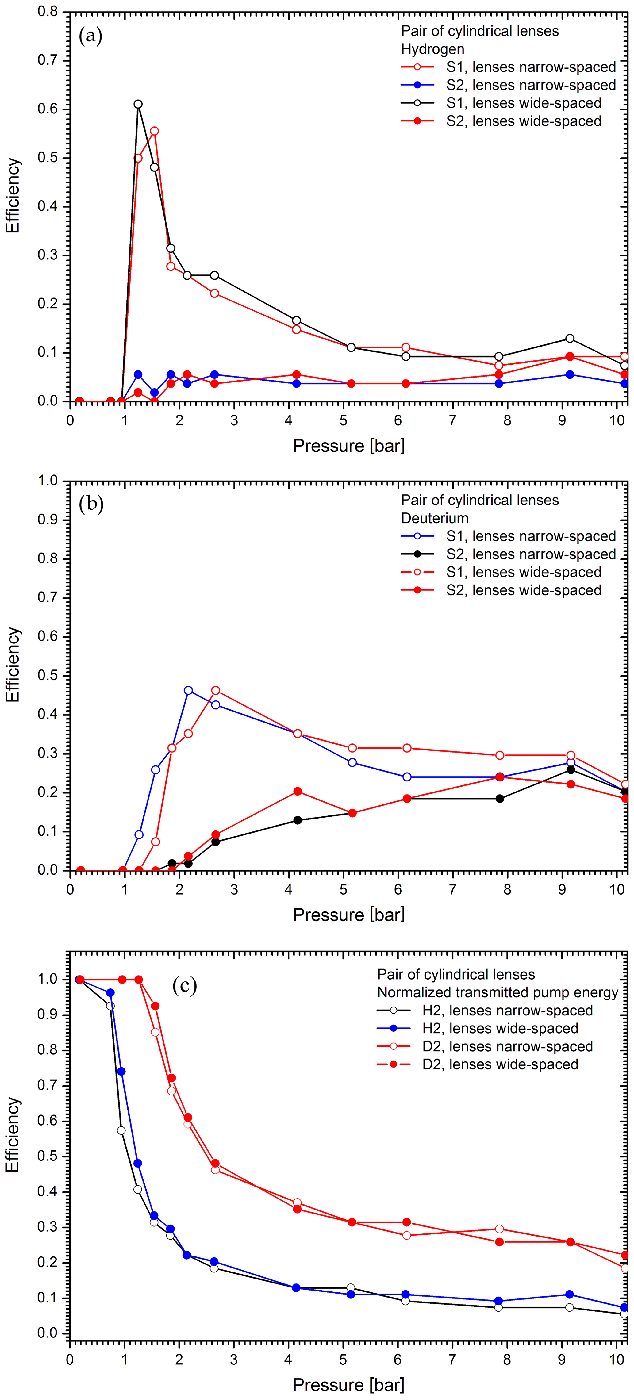
Figure 6Raman conversion efficiencies and pump beam depletion for a pair of crossed f=1.0 m cylindrical lenses: (a) S1 and S2 in hydrogen; (b) S1 and S2 in deuterium; (c) normalized transmitted pump energy in both H2 and D2.
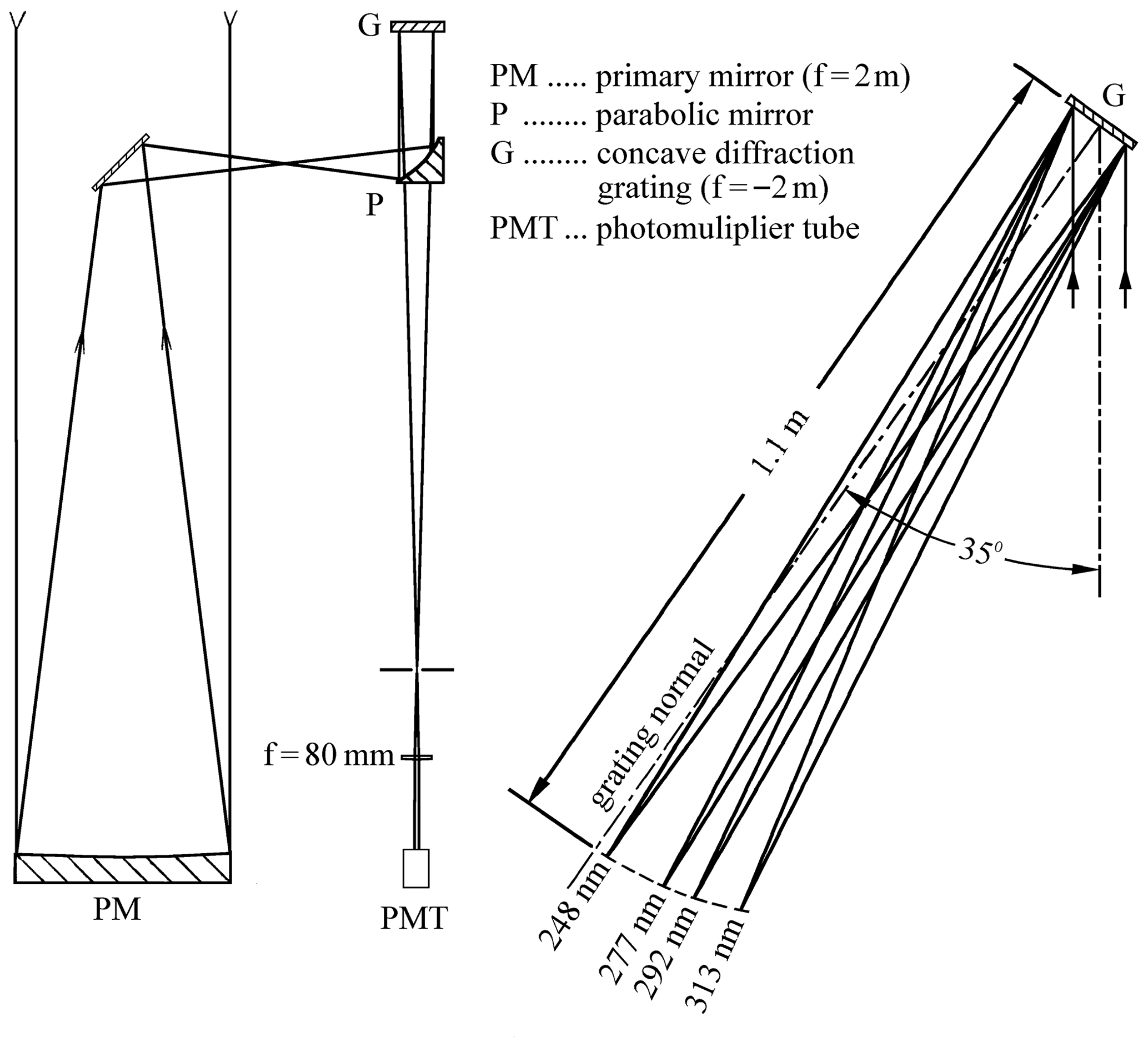
Figure 7Layout of the two grating spectrographs; α=35∘ is the Wadsworth angle chosen, corresponding to a wavelength of 240.0 nm. The choice of angle was limited by the space available in the housing of the spectrograph, also considering the big PMTs initially used.
The true spectral resolution was determined with a mercury lamp to be about 0.35 nm, achieved with low-intensity emission lines not exhibiting line broadening due to absorption in the lamp prior to emission. Due to the defocusing caused by the beam walk the effective spectral range for the components of the integrated lidar return is 1.0 nm (full-width at half-maximum, f.w.h.m.), but with sharp edges. The grating efficiency was specified as 70 % by the manufacturer (Carl Zeiss, Oberkochen) in auto-collimation, which may be different for the Wadsworth configuration.
An aperture with four adjustable blades (custom-made by OWIS) was placed at the entrance of each spectrograph in the focal plane of the primary mirror for reducing the level background light. In the large receiver the vertical blades were adjusted to block the near-field return and to transmit the return from all longer distances. These vertical blades were never touched again, and the laser-beam-steering mirror was always set for a peak signal at 8.0 µs. The horizontal blades are set for a slit width of 2–3 mm, after alignment with a narrow slit. The minimum slit width possible for S1 radiation is 0.7 mm (0.35 mrad), with more being needed for the S2 components. The consequence of the small spot size is a low susceptibility to typically observed laser pointing drifts, and the 277 nm return always yields correct ozone values.
Further adjustable slits (widely open) were placed in the secondary focal planes in front of the PMTs. However, this was just for occasionally controlling the alignment since no cross-talk between the different wavelength channels was observed. As mentioned, no alignment drifts were found.
As already mentioned in Sect. 3.1 the lidar signal varies with the polarization angle of the laser (Fig. 4). An approximate 5:1 sinusoidal modulation is seen. The polarization angle was set for optimum signal.
4.3.2 Mobile system
The polychromator design for the mobile system is quite different and is based on dielectric mirrors, beam splitters, an edge filter, and adjustable-slit apertures (Fig. 8). The 289 and 289 nm returns were separated by temporal discrimination, triggered by the rotating beam splitters described in Sect. 3.2. The data were stored in different areas of the transient digitizers. The separation of the larger gap between 266 nm and the two longer wavelengths could be conveniently achieved by pairs of dielectric beam splitters (BS3), each of them transmitting just 3 % of the longer wavelengths and fully reflecting the 266 nm component at an incidence angle of 45∘. In this way, two 266 nm channels were available for both the near- and far-field sections of the polychromator. As seen in Fig. 8, the entire arrangement is highly symmetrical and almost identical for the near- and far-field parts. A 1:100 beam splitter and an o.d. 1.0 neutral density filter (Andover) were used to separate and to attenuate the near-field return. In the far-field section the signal was first adjusted to perfectly match the near-field signal for low PMT gain. After this procedure, OWIS adjustable-blade apertures (see above), placed in the focal planes in front of the PMTs, were used to cut off the strong near-field return that was shifted horizontally (due to the perpendicular geometry of the outgoing laser beam, the telescope axis, and the telescope output axis). Finally, the PMT gain was increased to maximize the far-field signal. This approach is a rather simple alternative to the use of two telescopes as done in our stationary system and is also applied in our water vapour DIAL (Vogelmann and Trickl, 2008). However, it requires very constant pointing of the outgoing laser beam in order to avoid changes in signal level. This was not exactly the case for the laser used here but could be verified for the more recent (precision) version of the Powerlite laser of the H2O DIAL.
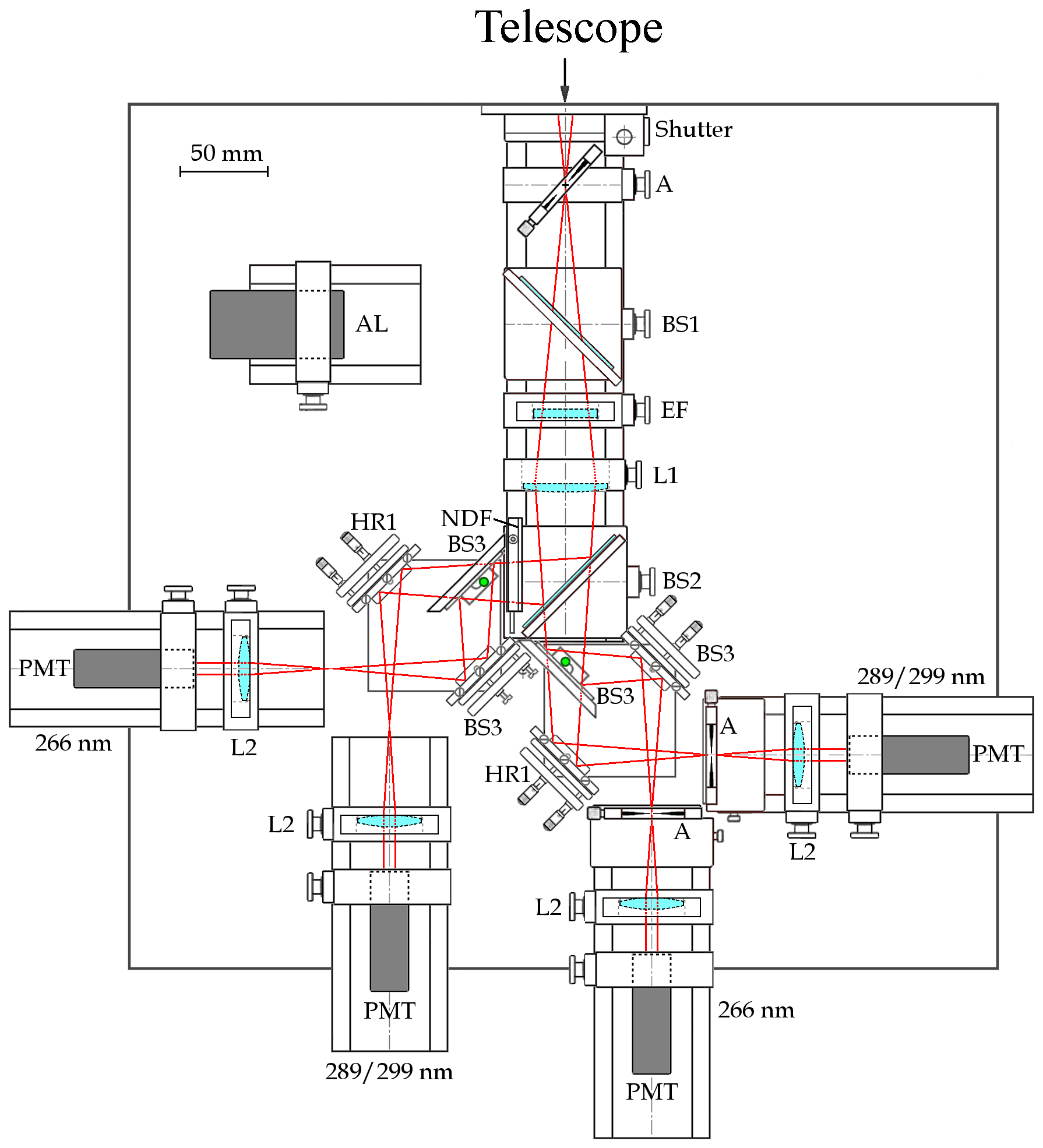
Figure 8Polychromator of the mobile ozone DIAL: the opto-mechanical components were mounted on a rail system attached to a black optical table with a 25 mm × 25 mm hole pattern (M6 threads, not shown). The two green dots mark the intermediate image planes of the primary mirror of the telescope (the secondary image planes coincide with the PMT cathodes). Abbreviations are as follows. A: rectangular aperture with four adjustable black blades; BS1: beam splitter for reflecting 532 or 1064 nm out of the received radiation for aerosol measurements (not implemented); BS2: 1:100 beam splitter for near-field–far-field separation; BS3: dichroic beam splitter with T<4 % for 289 and 299 nm; HR1: high-reflecting mirror (45∘); EF: dielectric edge filter, blocking the radiation above 299 nm; NDF: T=10 % neutral density filter; L1: f=100 mm lanes; L2: f=50 mm lens; AL: alignment laser.
An OWIS adjustable-slit aperture was also placed in the focal plane of the telescope (top of Fig. 8) for the reduction of the solar background. To account for the changing position of the “focus” as a function of the changing position of the outgoing laser pulse the orientation of the slit was horizontally tilted (i.e. perpendicular to the orientation in the stationary system due to the 90∘ rotation of the telescope exit). The vertical blades of the aperture could be closed to 1.7 mm (corresponding to an acceptance angle of 1 mrad) without a loss of signal but were set slightly wider during normal operation.
Each of the four detection channels principally look the same, apart from the different surfaces of the components (HR1, high reflector for 266 nm; BS3). As mentioned, the set-up deviates from the conventional modular set-up with relay-imaging lenses. The f1=100 mm ocular (L1) does not collimate the lidar return: it directly refocuses the radiation to an intermediate focal point. In this way, the overall distance to the detectors could be shortened. Just one additional lens (L2, f2=50 mm) was used for exactly imaging the principal mirror of the telescope onto the photocathodes of the PMTs. Most optical components were placed in the vicinity of the intermediate images of the primary mirror (green dots in Fig. 8).
One deficiency that was never overcome before the destruction of the system was that just a single PMT was for both on and off channels in the far-field section. Since the on signal peak is already rather small at the beginning of the far-field signal, the off component should be attenuated e.g. by rotating quartz plates with two differently coated halves similar to those next to the Raman shifter. This would allow the off signal to be reduced to about the same level as the on signal, and a higher PMT gain could be used.
4.4 Detectors
The detectors are key components of our lidar development, which calls for an explicit description. As suggested by Kempfer et al. (1994), we exclusively used the 14-stage EMI 9893B photomultiplier tubes (PMTs) between 1994 and April 1996. For linear performance the 9893B detectors were operated with maximum analogue signal levels below 10 mV (50 Ω termination). This means that the very high gain of this 14-dynode PMT (up to 8 decades) is completely unnecessary. The big plus was range gating (Kempfer et al., 1994), lifting the far-field signal level to values mostly well above the electronic imperfections of the signal processing system. The range-gating circuit was further improved for repetition rates of more than 20 Hz.
However, after very positive testing in 1995, we introduced Hamamatsu H5783P-06 PMT modules to both DIAL systems in spring 1996 (Brenner et al., 1997; Eisele and Trickl, 1997). The miniature PMT features a built-in Cockroft–Walton power supply, an 8 mm diameter photocathode, and six mesh dynodes, leading to a maximum current gain of 3×10⁵. This gain is sufficient for obtaining a very big lidar signal. This module is extremely linear over at least 5 decades for analogue signals up to at least 100 mV (50 Ω termination) in the operating voltage range around the most recommended 800 V. Fluorescence-free Corion SB-300-F short-pass filters were placed on the PMTs and efficiently removed radiation for wavelengths beyond 320 nm.
The small size of the modules allowed us to achieve a very compact design of the polychromators of the two lidar systems. In particular, side-by-side operation of all three PMTs in the spectrographs of the stationary DIAL became possible. These modules were used in our stationary system for more than 15 years without discernible signs of ageing.
Finally, driven by the hope for further improvement, we replaced the Hamamatsu H5783P-06 modules in 2012 with an actively stabilized version optimized for us in 1999 for our three-wavelength aerosol lidar (Kreipl, 2006) by Romanski Sensors (RSV). This device had to be based on the follow-up PMT version Hamamatsu R7400U-03 because the 5600 series was longer available. The socket was further modified to deliver optimized single-photon spikes without the ringing of the original PMTs (Fig. 9a and b). The power connection cable is shielded, but the shield is grounded just on one side.
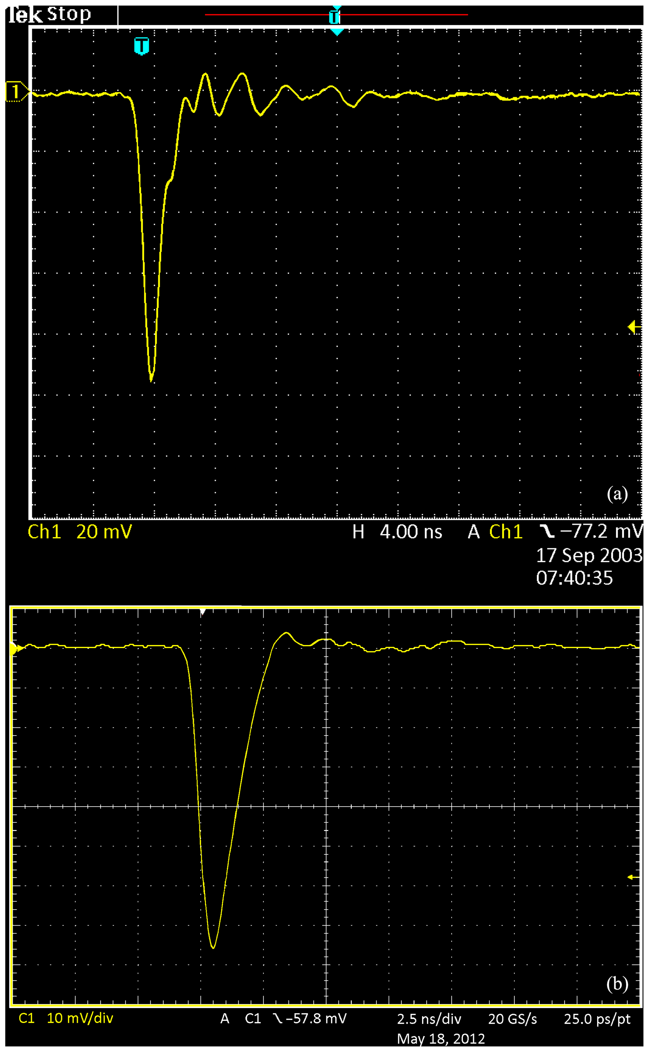
Figure 9(a) Single-photon pulse from a Hamamatsu 5600 or 7400 PMT, measured with a 500 MHz digital oscilloscope (Tektronix, TDS 3045 C). (b) Single-photon pulse from a Hamamatsu R7400P-03 PMT with the most recent version of the Romanski (RSV) socket, measured with a 1 GHz digital oscilloscope (Tektronix, DPO 7104).
Similar to the Hamamatsu module the RSV socket generates a clean reference voltage (5 V). This voltage is produced from the 15 V supply voltage. The 5 V reference, corresponding to a PMT voltage of 1000 V, is then returned to the power supply where it is divided to the adjustable final control voltage level (0 to 5 V) that is sent back to the detector (Fig. 3.12 of Kreipl, 2006). This loop was necessary to clean the lidar signals to a level below 10−5 of the peak signal. Sending in just an external control voltage resulted in an unacceptable baseline crossing of about 10−4 of the peak lidar signal.
The diameter of these detector modules, 50 mm, was too large for operating the PMTs for 277 and 292 nm side by side in the spectrograph of the stationary system. In order to make this possible, RSV delivered four of the modules with the small PMT tubes mounted off-axis.
Testing of the PMTs in our three-wavelength aerosol lidar showed that above peak signals of 40 mV signal-induced nonlinearities become observable that are attributed to photocathode overload (Fig. 3.10 of Kreipl, 2006; English version: http://www.trickl.de/PMT.PDF, last access: 19 November 2020). However, this result was obtained for a PMT supply voltage of the order of just 450 V and therefore corresponded to an excessive photon flux (see Fig. 10 for a gain curve). For voltages around 800 V (maximum: 1000 V), as recommended for photon counting, the incident radiation levels for creating the same signal are roughly 100 times lower. As a consequence, much higher signal levels can be afforded, and in recent years we have routinely set the peak signals in the far-field receiver to 70 mV, this being a rather conservative choice. This setting was motivated by the decision to stay within the 100 mV input range of the transient digitizer (Sect. 4.5).
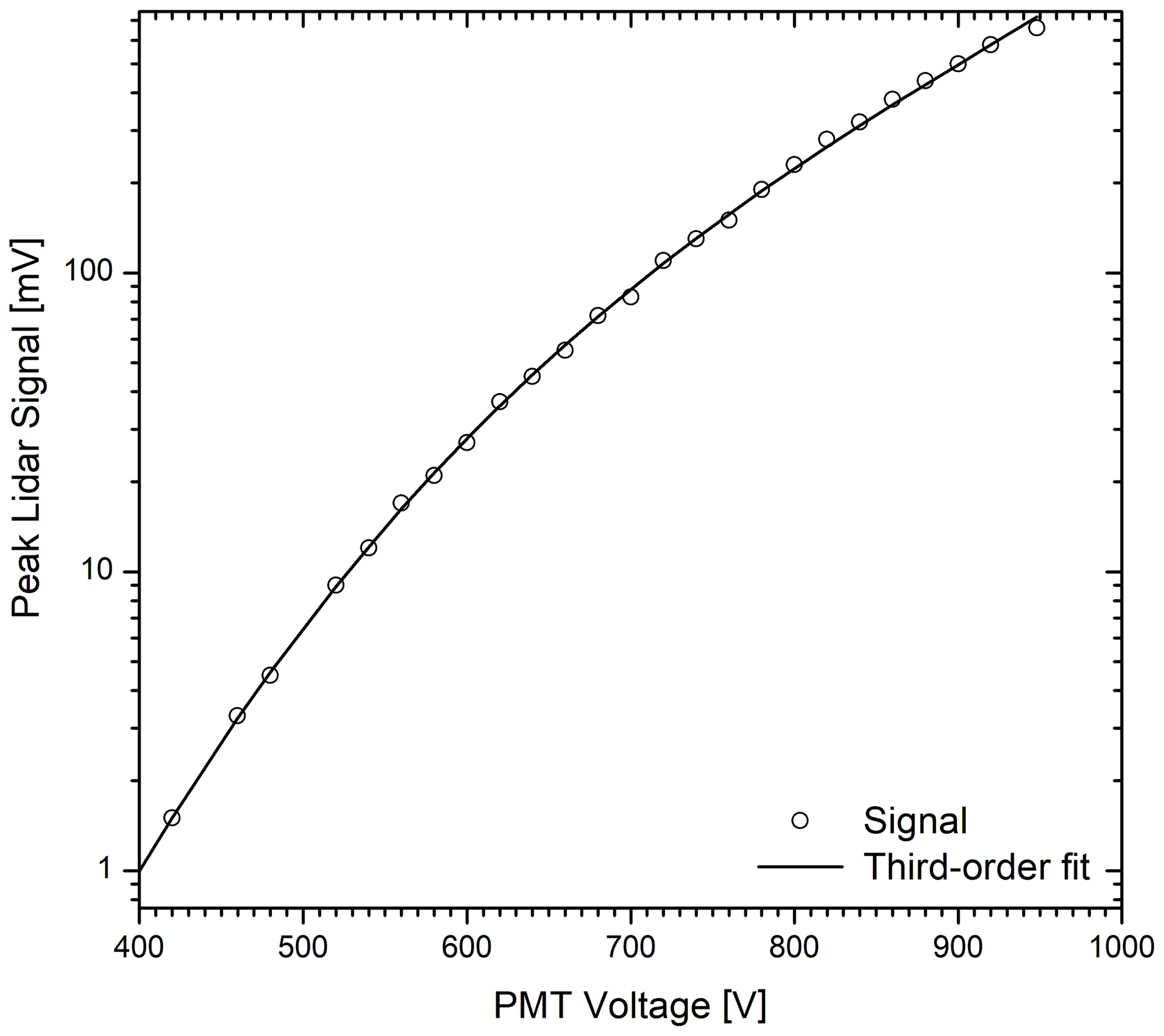
Figure 10Peak lidar signal measured with an R7400P-03 PMT as a function of the supply high voltage. The measurement was made for different attenuations of the incoming radiation by calibrating the data to the results for the standard settings. Signal-induced nonlinearities were only observed for very high photon fluxes, for which the supply voltage had to be reduced to 450 V to ensure signals below 100 mV (Kreipl, 2006).
We ascribe this unprecedented performance to the mesh layers of the dynode stages that likely act as electrostatic kinetic energy filters for the electrons. A pulse-height spectrum of one of the PMTs for the recommended operating voltage of 800 V is shown in Fig. 11. This spectrum was derived from a time scan with a 1 GHz digital oscilloscope (Tektronix, DPO 7104). No rise in photon counts towards 0 V pulse height is seen that would indicate signal-induced cathode emission, this result being limited by the chosen trigger level of the scope of −1.5 mV. It is important to mention that the pulse-height distribution does not end at −23 mV. As can be concluded from Fig. 9a and b, much higher pulses exist that can reach almost −200 mV. For 1 h measurements with our Raman lidar (Klanner et al., 2020) we did not observe dark counts in 7.5 m bins for discriminator thresholds of 4 mV and PMT supply voltages beyond 900 V.
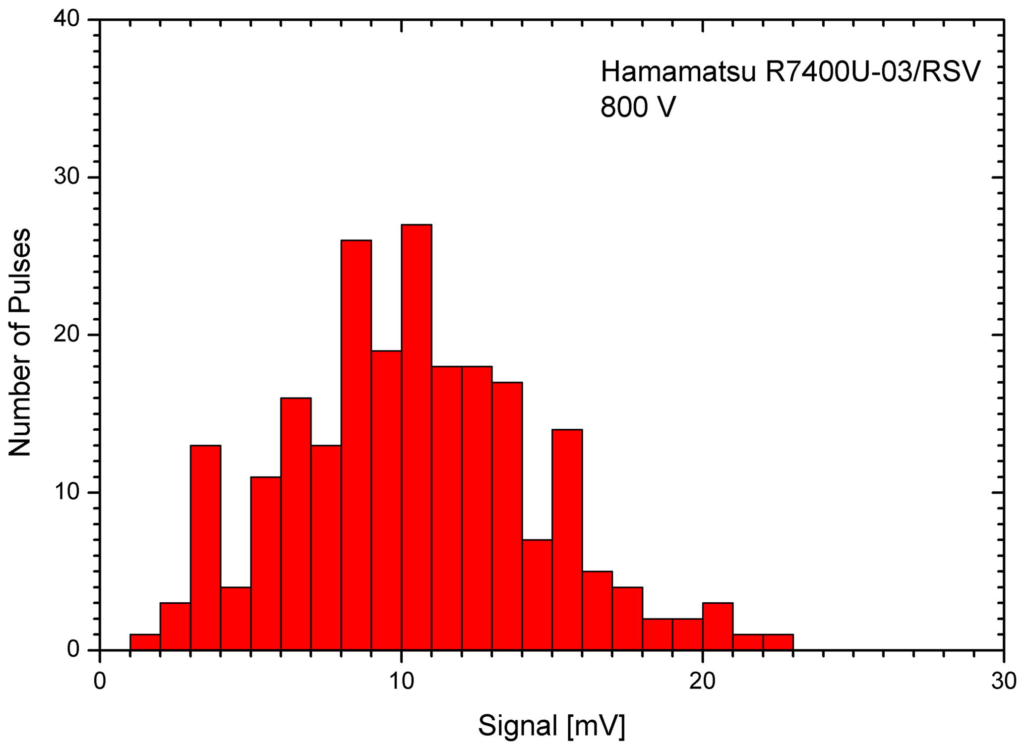
Figure 11Pulse height distribution of a Hamamatsu R7400-03 PMT (RSV module) for 800 V of operating voltage determined from a long time scan with a 1 GHz digital oscilloscope (sign of the pulse amplitudes inverted).
In the far-field receiver we found that a high number of photons is more important than a high peak analogue voltage because the photon noise dominates the signal at large distances. Thus, we no longer attenuate the signals and irradiate the photocathode with all the light emerging from the spectrograph. For compensation we reduce the PMT voltage to about 700 V. Now, the 70 mV signal level corresponds to about 2.5 times more photons per time interval than before. This change has resulted in considerable lowering of the ozone noise for the 292–313 nm wavelength combination in recent years. Photon counting at 700 V, along with the resulting much lower single-photon amplitudes, has not been tested so far (Sect. 4).
A really bad surprise was that the 7400 PMT is more than 1 order of magnitude more susceptible to daylight than the old modules. The H5783P-06 modules stayed linear up to about 12 mV of constant-background analogue signal. Now, the constant signal background must be kept below 1 mV. This task is demanding at 313 nm during the brightest part of the day, aggravated by the degraded surface of the primary mirror and in the presence of clouds. In spring and summer signal undershoot to below the signal baseline has even been observed during the hours around noon. We added a 5.7 nm (f.w.h.m.) filter from Laseroptik for additional background blocking. Still, mathematical corrections had to be made, which were particularly important for optimum aerosol retrievals. A filter with a 0.5 nm flat top and very steep edges is needed. Additional solutions could be an additional light baffle above the telescope and replacing the aged primary mirror of the telescope.
4.5 Transient digitizers
For the digitization of the analogue signal a 12 bit transient digitizer was found to be sufficient for avoiding the influence of single-bit steps since the shot-to-shot noise is larger than a least significant bit (LSB). This was anticipated by numerical simulations with artificial noise before the 1994–1995 upgrading of the stationary system that demonstrated the absence of steps for a noise amplitude of 4 LSBs. A sawtooth generator built for randomizing the single-bit steps turned out to be unnecessary. By contrast, Langford (1995) reported a significant improvement in his system achieved by modulating the signal.
In the upgraded stationary system, a 12 bit, 20 Hz system from DSP Technology was used until 2003. Since the mobile system was built 1 year later, the first 12 bit, low-noise 20 Hz transient digitizers systems from Licel became available and were used. The performance was excellent with lower noise than in the DSP system. In 2013, the Licel transient digitizers were upgraded at our request by introducing custom-made ground-free input amplifiers. This latest version has led to an unprecedented performance with a relative noise level of about of the full 100 mV voltage range after minor smoothing (Sect. 7.1), also yielding highly sensitive aerosol measurements at 313 nm despite the short wavelength. This unprecedented performance has made it possible to operate the system without photon counting with very little loss of quality.
Though being much noisier, the DSP Technology system was more linear than that of Licel as resolved down to a level of of the full scale (Kreipl, 2006; Fig. 3.10: http://www.trickl.de/PMT.PDF, last access: 19 November 2020). When firing the laser of our mobile aerosol lidar nearly horizontally onto a rock at a distance of 9 km, where the peak equalled the signal maximum, the return from beyond the rock instantaneously and exactly returned to zero. By contrast, the Licel system yields a small undershoot for distances beyond remote clouds that is larger for larger signal areas. Of course, the performance is perfect in the absence of clouds that generate very pronounced spikes. The performance of the most recent version of the Licel system is discussed further in Sect. 7.1.
4.6 Pre-amplifiers
In order to lift the PMT output, typically around 10 mV for the old PMTs and 70 mV for those from Hamamatsu (into 50 Ω), to the coarsest range of the transient digitizers, adjustable-gain pre-amplifiers were used until 2011 (Analog Modules, model 351, bandwidth 4 MHz, gain-adjustable between 1 and 10). In two of the far-field channels (on wavelengths) these pre-amplifiers produced some very small ringing. Between 1997 and 2003 these problems were overcome by using photon-counting data. For many years of exclusively using analogue data the ringing had to be removed by mathematical corrections. The ringing and the additional noise finally completely disappeared after disconnecting the zero voltage. After introducing the latest (ground-free) version of the Licel input stage the pre-amplifiers were removed.
4.7 Photon counting
In the stationary ozone DIAL single-photon counting was applied between spring 1997 and 2003 with an FDC700 1 GHz photon-counting system from Optec. The signals were fully linear starting in the middle troposphere but produced extra counts at lower altitudes, presumably due to pile-up effects of the PMT ringing (Fig. 9a). The signal for photon counting was separated from the analogue output by an impedance-matched junction containing an adjustable discriminator custom-made by RSV. In the first version the discriminator level could not be reduced to below 11 mV. This level had to be chosen to ensure linear performance and maximum signal (Fig. 11). The unit was upgraded several years ago for picosecond time resolution and discriminator levels down to 2 mV.
The new PMT units delivered by RSV are free of the ringing of the original Hamamatsu tubes (Sect. 4.4) and feature pulse widths of about 1.5 ns (Fig. 10). In order to benefit from this considerable time resolution we recently purchased MCS6 and MCS6A five-channel high-speed photon-counting systems from Fast Comtec for several of our lidar systems. The signals are scanned for selectable pulse edges at intervals of 100 ps, which means a maximum count rate of about 5 GHz for equidistant picosecond pulses. For both reasons a highly linear photon-counting performance was achieved that is presented in detail in the parallel publication on our Raman lidar for water vapour and temperature (Klanner et al., 2020).
The simultaneous analogue and photon-counting measurements from a single PMT lead to a deterioration of the analogue signal with an artificial perturbation of the signal of the order of 10−4 of the peak voltage. This could be reduced by 1 order of magnitude by adding an optocoupler to the trigger input of the counting system. However, the shape of the perturbation was somewhat complex and thus difficult to correct mathematically. In addition, we do not have experience with photon counting at the currently preferred PMT voltages of around 700 V or less (see above). At this time the simultaneous application of photon counting is postponed until a better solution becomes available.
4.8 System control
All connections between electronic components of the two DIAL systems are ground-free. The trigger pulse is derived from a photodiode and subsequently distributed into numerous output channels via optocouplers (Ingenieurbüro W. Funk). The supply voltages for the PMTS, pre-amplifiers, and discriminators (Ingenieurbüro W. Funk) are generated through high-quality DC–DC converters (TRACO POWER, models TYL 05-05S30 and TYL 05-15W05). They are transferred to the different devices in shielded cables. The shields of the cable leading to the PMTs are open on the side of the detectors. The supply voltage can be set by the lidar PC via an I2C bus, but this option has never been used in the stationary system because of the rather stable clean-air conditions at Garmisch-Partenkirchen. Also, the opening and closing of the flap in the roof was initiated via an I2C bus.
Electromagnetic interference from outside (e.g. the laser) has been kept at a negligible level by using doubly shielded signal cables (Suhner, G03332; the outer shield is left open on one side) and ground-free circuits. The trigger pulses were obtained from photodiodes and then distributed via optocouplers.
The firing of the XeCl laser was initiated via RS232 remote control of the computer of the excimer laser. The power for the high-voltage circuits of the laser is supplied by a separate source. The laser PC was connected to the clean power in the lidar laboratory. The laser itself is controlled by its computer via optical fibres. Finally, both cables connecting the lidar laboratory and the laser PC are shielded, which successfully removed any interference from the high-voltage pulses (Eisele and Trickl, 1997).
4.9 Automatic operation
Both DIAL systems have been extensively operated under automatic control by the lidar PC. In the mobile system an external start and warm-up of the laser was not possible due to issues in the programmes delivered by Continuum. The laser output was continuously controlled: the measurements were interrupted if the 1064 and 266 nm power levels were below maximum.
Among the various error conditions the most important ones are rain and high wind speed. This results in an immediate closing of the flap in the roof. As to the KrF laser the high-voltage is shut down, and as to the Nd:YAG laser the output shutter is closed, with the laser continuing to fire in order to maintain thermal equilibrium of the frequency-doubling crystals.
Time series under automatic control have been extended for the stationary system to up to 4 d. In this way, numerous atmospheric transport studies could by made, with the first 4 d series leading to the first detection of North American ozone over Europe (Eisele et al., 1999; Trickl et al., 2003).
The number density of ozone, , is obtained by computing the DIAL equation,
with the difference
of the absorption cross sections of ozone. P is the power returning from the atmosphere (“lidar signal”), β the total backscatter coefficient, and αr the residual extinction coefficient that includes Rayleigh and particle scattering as well as absorption by molecules other than ozone. In the absence of aerosols and interfering gas Eq. (1) reduces to
with the subscript R denoting “Rayleigh”. The Rayleigh extinction coefficients can be calculated in the ultraviolet spectral region with relative uncertainties less than 1 % if radiosonde data are used for deriving the atmospheric density. For short on wavelengths (266 nm, 277 nm) the absorption of the radiation by ozone dominates the extinction coefficients, and thus the uncertainty due to the Rayleigh term is negligible.
Under the clean-air conditions prevailing at Garmisch-Partenkirchen Eq. (2) is a mostly reasonable approximation. However, occasionally aerosol corrections must be made. Due to the large wavelength separation in UV ozone DIALs, the inference by aerosols may contribute more seriously than in DIAL systems measuring species with a well-resolved line structure allowing the use of neighbouring wavelengths. Operational procedures based on an iterative parameter search were developed that are described in detail in our preceding publication (Eisele and Trickl, 2005). For calculating ozone in the presence of structured aerosol distributions the lowest errors have been obtained for the wavelength pair 277–292 nm, followed by 277–313 nm and 292–313 nm. The most important factor is a strong absorption cross section of ozone and then a minimum (but finite) wavelength difference (Völger et al., 1996; Eisele and Trickl, 2005), in contrast to a frequently heard, but obviously wrong, opinion.
Our numerical approach was significantly modified with respect to that published earlier (Kempfer et al., 1994). Previously, the derivatives in the DIAL equation were calculated by fitting third-order polynomials to the backscatter profiles within a given evaluation interval. This method worked rather well but was slow. A faster modified approach resulted in small steps in the generated ozone profiles, requiring the application of some moderate data smoothing in addition (Kempfer et al., 1994).
From the point of view of numerical filter theory polynomials are not ideal because their transfer functions expose ringing. We decided to calculate the derivative with a simple linear least-squares fit of just a short interval, keeping the vertical resolution (see further below) at about 50 m, followed by optimized numerical filtering. A five-step algorithm is applied, consisting of
-
data pre-smoothing at a level roughly corresponding to the chosen minimum vertical resolution of 50 m (important for smooth aerosol retrievals for the near-field telescope),
-
calculation of the derivative with a constant number of data points in a sliding interval,
-
range-dependent data smoothing with a vertical resolution of about 50 m at low altitudes and 250 to 500 m in the tropopause region, depending on the noise level of the respective measurement,
-
truncation of the uppermost ozone profiles at an altitude below the onset of diverging noise, in summer sometimes even below the tropopause, and
-
final minor smoothing of the composite ozone profile put together from the best segments of the partial ozone profiles from different wavelength combinations and the two telescopes.
The smoothing intervals in step 3 have been mostly minimized in order not to suppress existing ozone structures.
For a linear fit and equidistant data points the result of the fits may be expressed in a rather simple formula, resulting in the following solution of the DIAL equation for the ith data point (Vogelmann and Trickl, 2008). Selecting a fit interval between data point i−k and i+k, one obtains
with the signal ratio
with Δr being the size of the range bin of the transient digitizer or photon-counting system. Application of Eq. (3) allows a fast computation of the derivative, in particular for constant k, when only the sum in the numerator must be calculated for each step. In Eq. (3) < qi> is written instead of qi as by Vogelmann and Trickl (2008). This is explained further below.
Another important advantage of Eq. (3) is that the least-squares fit is not applied to the logarithm, but to the signal ratio itself, due to the transformation
In contrast to the noise of the logarithm of qi the noise of the signal ratio is symmetrical and fulfils a key prerequisite of least-squares fitting. A negative density ozone bias is therefore avoided.
However, the application of Eq. (3) has limitations. Its application to simulated lidar profiles revealed that there are numerical biases with growing interval sizes 2k. This is further discussed below.
The linear approach in Eq. (3) is reasonable for interval sizes L=2kΔr not exceeding a scale representing the ozone distribution. Equation (3) is a reasonable choice for data smoothing, but it is not a perfect frequency filter and transmits residual high-frequency noise. Therefore, we have used a combination of Eq. (3) in a limited interval and numerical low-pass filtering.
Numerical low-pass filtering of data points yi is based on the general equation (Eisele, 1997, and references therein)
with the smoothed value and the coefficients
with fc and fs being the cut-off and sampling frequencies, respectively, and N a normalization factor. The interval width is . One general problem with numerical low-pass filtering is the occurrence of ringing. This can be minimized by introducing window functions wj,
After comparing several listed window functions a Blackman-type window (Blackman and Tukey, 1959) was chosen:
The best performance was achieved by selecting
with c being the speed of light. The response function obtained for applying Eqs. (5)–(7) with k=25 is depicted in Fig. 12 together with that for a sliding arithmetic mean over symmetrically arranged data points. A linear least-squares fit is equivalent to the arithmetic mean. These linear operations, though suitable for smoothing, are not perfect frequency filters and therefore transmit residual high-frequency noise. More details on the frequency transfer functions for some filters are given by Eisele (1997) and, more recently, by Iarlori et al. (2015) and Leblanc et al. (2016).
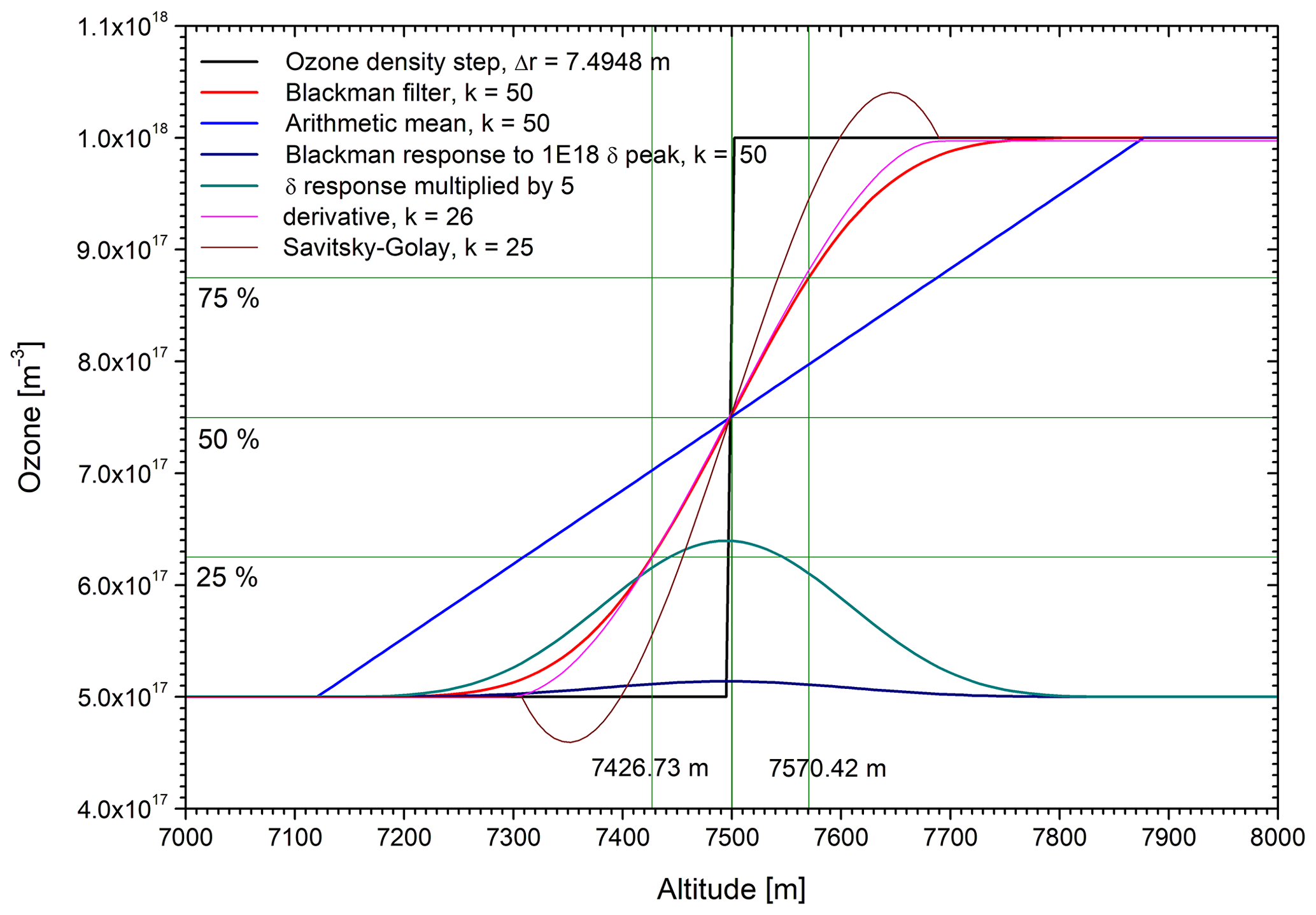
Figure 12Response of the digital filter used in the data evaluation procedure for the IFU DIAL systems to a Heaviside ozone step and for a sliding arithmetic mean; both filters are shown for smoothing over 101 points, and a digitizer bin size of 7.4948 m is assumed. The VDI vertical resolution is the altitude difference for a rise from 25 % to 75 % of the input step. For comparison, the very small response of the Blackman filter to a delta (single-bin) signal peak of 1×10¹⁸ residing on a 5×10¹⁷ background is shown, with the enhancement also multiplied by 5. The slope for a k=27 derivative filter (see text) is identical to that of the Blackman filter at half-rise. Finally, the result of k=25 Savitsky–Golay smoothing is shown, 25 being the maximum possible k value in the ORIGIN graphics package. This kind of smoothing is absolutely inadequate.
The vertical resolution can be defined in a number of ways (Iarlori et al., 2015; Leblanc, 2016). For practical reasons the German Engineering Society (Verein Deutscher Ingenieure, VDI, 1999) introduced a definition of the range resolution as the interval between 25 % and 75 % of the rise in the response to a Heaviside step (Fig. 12). Here, the response reaches a signal level of 100 % at large distances from the step. Since the VDI guideline was published we have preferred to apply this definition. In spectroscopy, the spectral resolution is preferentially defined as the full-width at half-maximum of the response to a delta peak. As we can see in Fig. 12, without normalization the delta response is much smaller than the original one, which looks strange in practice.
From Fig. 12 we derive for the Blackman filter a VDI vertical resolution of 19.2 % of the full filtering interval L. The response of the Blackman filter to a single-channel (“delta”) peak (5×10¹⁷ m−3 to 1×10¹⁸ m−3) was found to exhibit a full-width at half-maximum of 34.3 % of L (Fig. 12). This fraction looks surprisingly large in comparison with the step response. The fractions for the pure Blackman filter (Eqs. 5, 6) are also valid for much smaller smoothing intervals than in this example.
We also give in Fig. 3 an example for numerical differentiation of a simulated lidar measurement based on Eq. (3). The DIAL equation was synthesized for the wavelength pair 277–313 nm based on the artificial ozone density step between bins 999 and 1000 and on an air density profile calculated from the U.S. Standard Atmosphere (1976). The absence of particles and absorbing molecules other than ozone was assumed. The application of Eq. (3) yields a similar step (Fig. 3) that matches that for the Blackman filter within most of the rise if one selects k=27. In contrast to an ideal filter the derivative filter transmits some residual noise. The VDI vertical resolution is about 45 % of the filtering interval (k=10 to 30, presumably in a wider k range).
It is important to note that due to the curvature of the backscatter profiles Eq. (3) yields a bias that is absent in the case of missing Rayleigh scattering. This bias grows with k and is negative for Eq. (3) (for k=27: −0.0050 × 10¹⁷ m−3 (−0.10 %) ahead of the step and −0.0033 × 10¹⁸ m−3 (−0.33 %) behind it). This bias is small, and it even becomes negligible for e.g. k=10 (and less). However, it grows with k. Thus, it is reasonable to use moderate values of k for the derivative and subsequent numerical filtering with Eqs. (5) and (6) to remove the residual noise. Finally, the use of qi instead on in the denominator of Eq. (3) yields a positive bias larger than the negative one for using Eq. (3). This justifies the choice of . One could think about an empirical mathematical correction interpolating between qi and .
The filter interval for the smoothing is dynamically enhanced with height by applying a linear relation for simplicity (a quadratic dependence might be better). The coefficients c1 and c2 are preselected for each wavelength pair:
For example, for the large telescope of the stationary lidar c1=0 ad c2=0.125 for the pair 277–313 nm and c1=0 and c2=0.156 for 292–313 nm. This results in filtering intervals 2 k of the order of 250 and 500 near the upper end of the respective useful range (VDI vertical resolutions of 360 and 720 m, respectively). These preset coefficients are used for the initially automatically produced set of quick-look profiles but are afterwards reduced in size in some subranges if allowed by the noise level. In ranges with clearly distinguishable ozone gradients (e.g. stratospheric intrusion peaks or tropopause) or strong narrow features, the vertical resolution is also reduced as far as reasonable. In particularly noisy subranges in the upper troposphere sometimes homogeneously distributed ozone is fitted to the corresponding density segments. The different segments are pasted into the actual overall ozone profile.
As a consequence of this complexity, a solution for automatically deriving uncertainties for all partial data segments has been postponed. In the early 1990s uncertainties for the much less sophisticated evaluation procedure was calculated from the least-squares fitting approach applied (Kempfer, 1992).
The calculation of mixing ratios and the retrieval of aerosol backscatter coefficients require knowledge of the atmospheric density. Within the troposphere this is not extremely important and simple annual average density profiles do not contribute more than a few percent to uncertainty (Carnuth et al., 2002). However, with growing data quality and a range reaching the stratosphere the incorporation of a better density profile became mandatory. This is achieved by importing the radiosonde data for the nearest station of the German Weather Service, Munich or Stuttgart, from the University of Wyoming database (http://weather.uwyo.edu/upperair/sounding.html, last access: 19 November 2020).
313 nm aerosol backscatter coefficients have been routinely calculated for each measurement since 2007 based on the methods mentioned above (Eisele and Trickl, 2005). They are publicly available for all years starting in 2007 from the EARLINET database (https://data.earlinet.org/, last access: 19 November 2020).
The quality of the aerosol backscatter coefficients for the latest period of lidar operation is extremely high during most of the day, as can be seen in Trickl et al. (2015) and in Sect. 7.1. This has served as an additional quality criterion for the ozone retrieval, together with the comparison of the DIAL profiles for different wavelength combinations and the single-wavelength ozone retrieval for 292 nm. In the absence of aerosol this single channel is extremely reliable and, in summer, less noisy than the DIAL solution for 292–313 nm. However, the Rayleigh backscatter coefficients must be calculated from radiosonde data in order to achieve good quality.
After the introduction of the 7400 PMTs, a slight correction of the far-field 313 nm profiles became necessary during the hours around noon (Sect. 4.4). The overshoot of the normally negative signal is particularly pronounced in summer due to the PMT overload effects in the presence of a daylight background exceeding 1 mV. Aerosol retrievals are mostly perfect during night-time; just a constant displacement of the order of 10−7 m−1 sr−1 must be corrected. As the 313 nm PMT starts to exhibit overshoot for large distances, a mathematical correction becomes necessary, in summer even before 10:00 CET. In the absence of aerosol in the upper troposphere and the lower stratosphere the corrections can be nicely verified by comparing the DIAL ozone with the 292 nm single-signal ozone retrieval.
6.1 Calibration
Since the first measurement series in 1991 the ozone data have been calibrated by using the absorption cross sections from the University of Reims (Daumont et al., 1992; Malicet et al., 1995). The motivation for this is described by Kempfer et al. (1994). Most importantly, the measurements account for the decomposition of ozone during the absorption measurements by precise pressure measurements. The cross sections have measured again and again (e.g. Gorshelev et al., 2014; Serdyuchenko et al., 2014, and references therein), but no improvement has been achieved, except for perhaps the temperature dependence. Very recently, four new cross sections measured between 244 and 254 nm at an uncertainty level of 0.1 % have been provided by Viallon et al. (2015). In view of the choice for our ozone DIALs it is extremely satisfactory that the agreement with the corresponding values in the Reims data is within ±0.06 %.
The temperature dependence as a function of altitude is obtained by interpolation of the cross sections from Reims measured for different temperatures.
6.2 Validation
For the convenience of data users, the system performance is summarized in Table 4 for the different periods of operation. The uncertainties have been derived from validation exercises, sensitivity studies in low-signal ranges, and noise estimates and reproducibility of the ozone densities during diurnal series of measurements.
The lidar system has been systematically validated (since 2007 on each sounding day) by using the in situ data from the nearby mountain stations Wank (1780 m a.s.l.) and Zugspitze (2962 m a.s.l.) until the measurements at these sites were discontinued (evaluated data are available until 2010). Afterwards, the ozone values of the Schneefernerhaus (UFS) Global Atmosphere Watch station have been used for occasional comparisons (Trickl et al., 2014, 2020). UFS is located on the southern face of Zugspitze at a distance of 9 km from the ozone DIAL at IFU. The gas inlet is at 2670 m. The average ozone mixing ratios are about 1 % lower than those at the summit (Ludwig Ries, personal communication). The lidar data agree similarly well with those from UFS as previously with the Zugspitze ozone.
In addition, a large number of successful comparisons have been made with the Hohenpeißenberg ozonesondes (distance: 38 km); a few examples were given by Eisele et al. (1999). A more extensive comparison is planned for the 2018 data, accompanied by a highly successful comparison with a sonde launched by colleagues from Jülich directly at IMK-IFU in February 2019. The latter side-by-side comparison for mixing ratios of about 50 ppb yielded a rather constant bias of the sonde of 2 to 3 ppb up to 7 km and, above this, a slightly higher variability of the differences.
These comparisons have certain limitations. In the case of the Hohenpeißenberg sondes the air-mass difference matters in certain altitude ranges due to a 48 km distance between the two stations. Under comparable conditions the differences between the profiles have been between 5 % and 10 %.
The lidar has shown a slightly positive bias with respect to the Wank site, mostly not exceeding 5 ppb. This bias is not present during night-time but mostly forms in the morning under warm conditions. It has therefore been ascribed mostly to slope winds (Carnuth and Trickl, 2000, Fig. 5) venting morning-type low-ozone air from the valley up this rather isolated summit that acts like a chimney. Frequently the summertime morning values agree better with the 05:00 CET measurement than with the Wank mixing ratio for the true data acquisition time. Until 2011 some alignment issues occasionally exist that enhanced the uncertainty for distances below 0.5 km. The Wank site has been invaluable for verifying good alignment of the near-field telescope, until 2011 with some resulting problems.
The comparisons with the Zugspitze in situ data have been mostly very convenient. The differences of the mixing ratio have rarely exceeded 2 ppb, with exceptions typically occurring if there is a pronounced ozone gradient around 3000 m. In the absence of an extended comparison since 2012 an example from a 4 d series in May 1999 (Trickl et al., 2003, 2011) is shown in Fig. 13 that exhibits more noise than recent comparisons. The data are compared for two lidar altitudes, 2970 and 2786 m. The lower altitude accounts for the air-mass rise during the final approach towards the high mountain. The results for 2970 m show a few positive departures that result in a positive average difference between the lidar and station of 0.82 ppb (standard deviation: 2.15 ppb). For the lower altitude the “bias” is just 0.34 ppb (standard deviation: 1.61 ppb). These values are all small in comparison with the average Zugspitze mixing ratio, but the sign agrees with the expectation for the 1.8 % bias of the in situ measurements obtained in the recent cross-sectional study by Viallon et al. (2015).
The performance of the mobile system is discussed in Sect. 5.5.
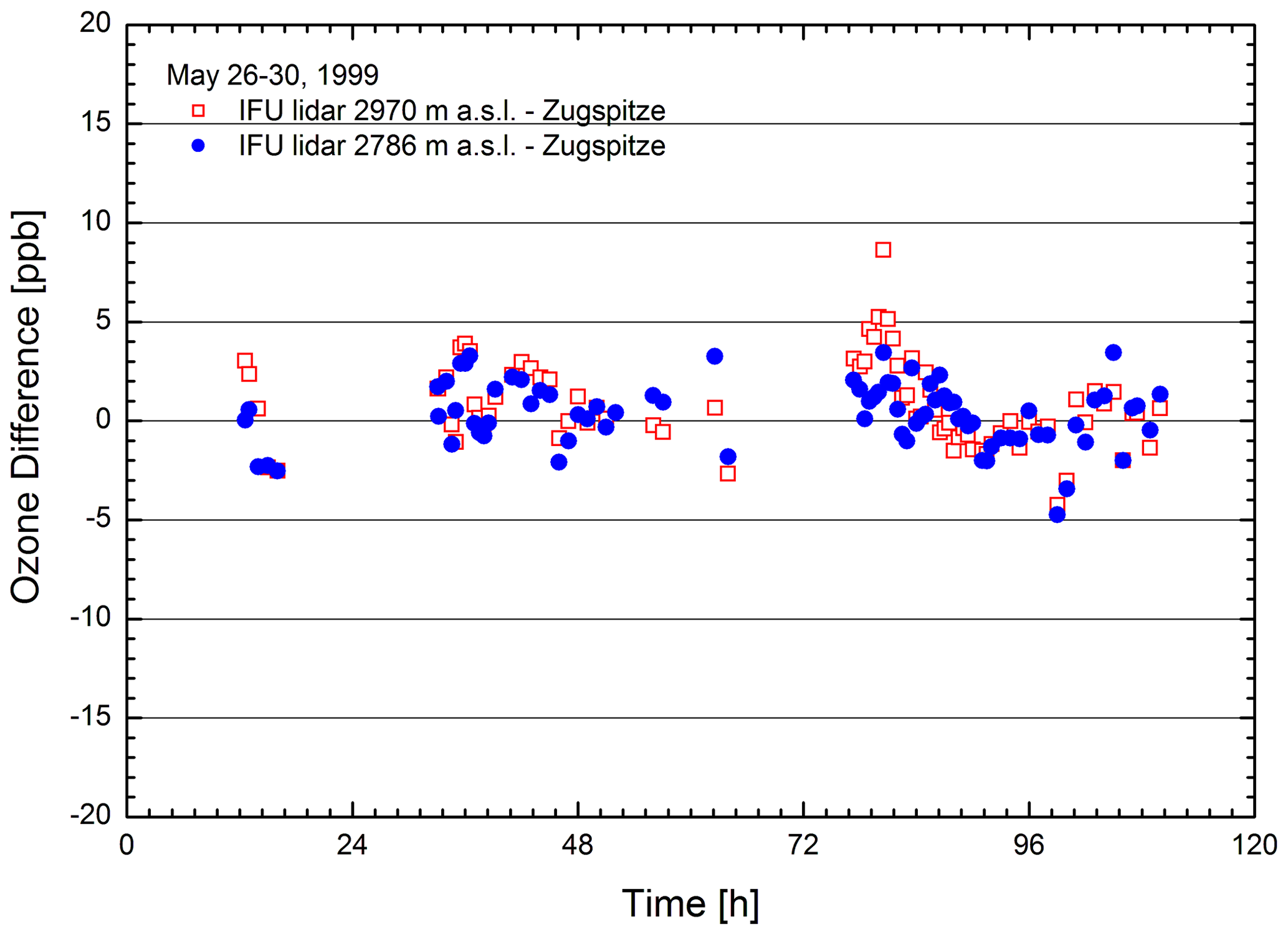
Figure 13Comparison of the stationary DIAL with the Zugspitze in situ data during 4 d in May 1999 (VOTALP Munich field campaign); the deviations have since diminished to about one-half of the noise shown here.
6.3 Interference by other gases
Important species absorbing in the typical wavelength range of ozone DIAL systems are SO2, NO2, and some hydrocarbons. Under the clean-air conditions prevailing at the Alpine site Garmisch-Partenkirchen and in the free troposphere, spectral interference from these constituents should be very rare. As mentioned, the mobile DIAL retrievals for the wavelength pair 266–299 nm are almost insensitive with respect to SO2 and NO2.
Oxygen must also be considered in the wavelength region below 285.66 nm (Krupenie, 1972; Jeunouvrier et al, 1999). The absorption cross sections of O2 in this region (Herzberg bands) are rather low, but absorption cannot be completely neglected due to the high concentration of this molecule. We found some approximate coincidences with non-relevant high rotational levels and an approximate coincidence of the 277.11 nm emission with J=5–7 components of the extremely weak (2,0) band. 266.12 nm is slightly outside a group of O2 lines. In summary, absorption of the emissions used in the two DIAL systems in oxygen can be neglected, in agreement with the good validation results.
7.1 Examples for the stationary system
After the first upgrading of the stationary DIAL in 1994 and 1995, the system yielded greatly improved sensitivity and a much larger vertical range up to about 15 km due to the three-wavelength operation. The number of measurements per year grew and time series under automatic control were extended up to 4 d, the first 4 d series being the well-documented one in May 1996 published by Eisele et al. (1999), Stohl et al. (2000), Cristofanelli et al. (2003), and Trickl et al. (2003). However, until 2003 the operation was limited to funded projects and focused research topics. After the second major system upgrading routine measurements were started in 2007. Almost 5000 ozone profiles were obtained from 1991 to February 2019, and numerous examples can be found in our publications (see the Appendix; the most recent one for the period 2007 to 2016 can be found in Trickl et al., 2020).
A summary of the work done is given in Table 3. Uncertainties estimated for the different periods and altitude ranges are specified in Table 4 as a guide for potential data users.
Table 3Measurement periods of the stationary DIAL.
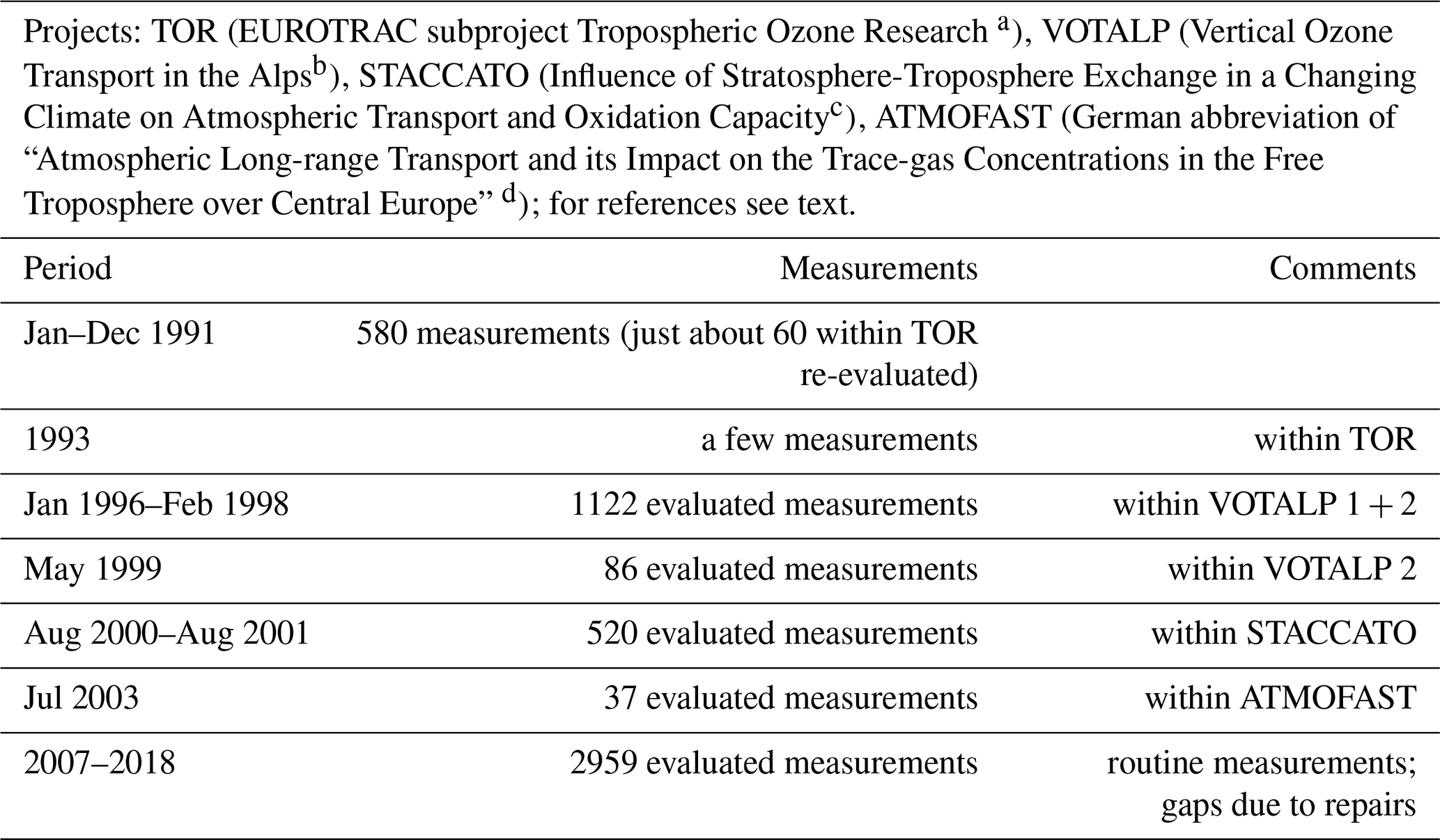
a Kley et al., 1997, b Wotava and Kromp-Kolb, 2000; VOTALP II, 2000, c Stohl et al., 2003, d ATMOFAST, 2005.
Table 4Uncertainties of the stationary ozone lidar.
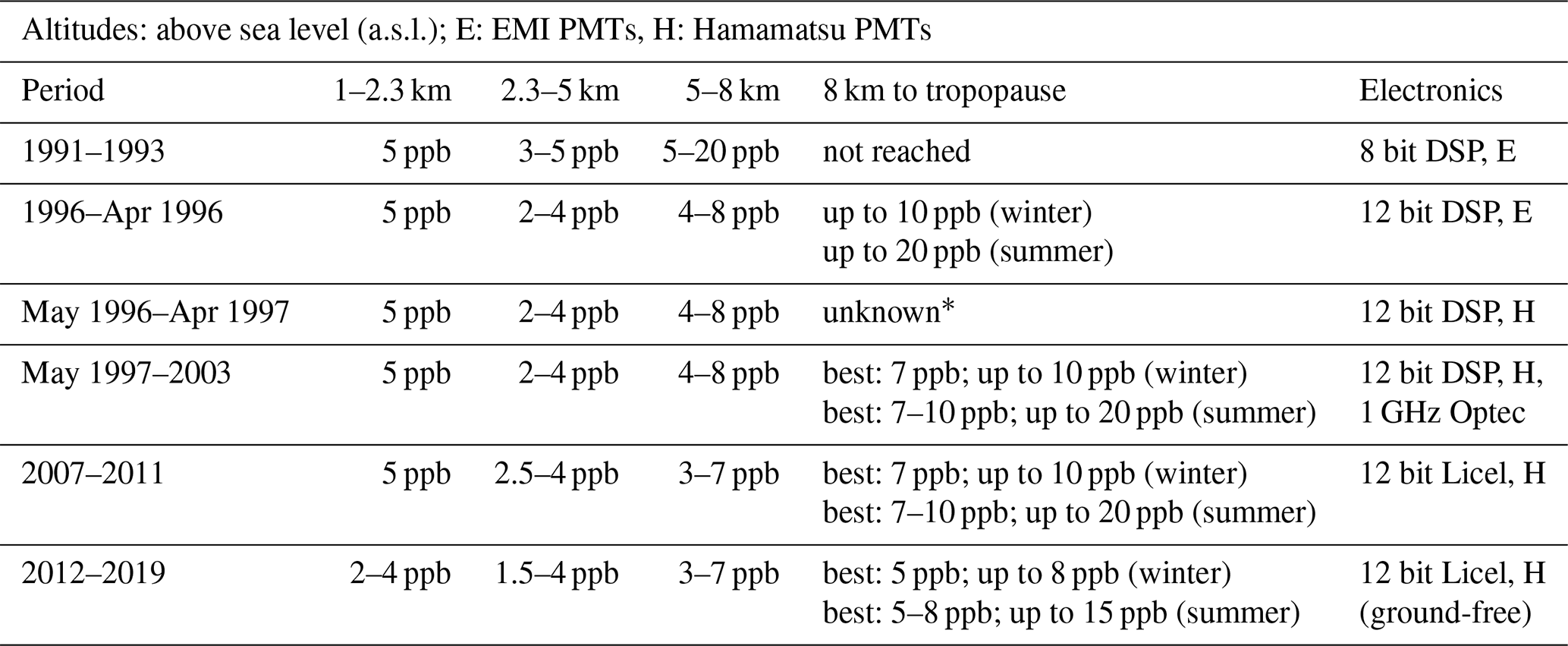
∗ Sometimes there are artefacts in the upper troposphere due to pre-amplifier ringing, which are corrected for important examples.
Figure 14 shows the raw backscatter signals (a) uncorrected and (b) with automatic exponential correction. The amplitudes of the corrections grow with the area of the backscatter signal, which is larger for the far-field telescope than for the near-field telescope, and grow with the wavelength due to the decreasing absorption cross section. In the range in which such an exponential wing affects the lidar signal it does not exceed a few times 10−5 of the input voltage range (100 mV). The slightly enhanced noise in channel 6 (313 nm, red curve) is caused by the early-morning daylight roughly 1 h after sunrise.

Figure 14Strongly expanded backscatter profiles without (a) and with (b) exponential correction, recorded after the introduction of the ground-free input stage to the transient digitizers in late 2012; the 313 nm signals are noisier due to the early-morning daylight background. The data are smoothed over ±14 points (VDI vertical resolution 40 m) in order to reduce the digital ripple.
The introduction of three-wavelength operation made possible an internal quality assurance. Ozone profiles are derived from different wavelength combinations. The observation of mutual deviations in the retrieved densities results in immediate re-examination of the alignment. As mentioned, just two misalignments matter: the overlap of the partial beams emerging from the Raman shifters after recombination and the pointing of the beam emitted into the atmosphere. Minor discrepancies for 292–313 nm due to alignment drifts during extended periods of unattended operation can be conveniently recalibrated by using the 277–313 nm profiles as a reference, which was routinely done in recent years. As mentioned, the 277 nm channel of the large telescope was found to be insensitive to slight misalignments, presumably due to the particularly small focal point in the entrance slit of the spectrograph. In addition, small drifts in laser pointing do not result in a transverse displacement of the spot on the detectors that are placed in the image planes of the principal mirror of the telescope.
One example of a measurement with a perfectly aligned lidar is shown in Fig. 15 (26 October 2015). The figure contains three ozone profiles from both receivers. The three ozone profiles match well in their common overlap regions. Nevertheless, due to low ozone the near-field signal (here 277–313 nm) yields reasonable ozone values up to 2.5 km above the ground (740 m a.s.l.). The range for the same wavelength pair in the large receiver extends up to 6.5 km a.s.l., with moderately elevated ozone. The simultaneously measured ozone value at UFS is lower by just 0.7 ppb. The 292–313 nm ozone profile exhibits less structure than that for 277–313 nm. The absorption cross section for 292 nm is less than one quarter of that for 277 nm, which necessitates smoothing the 292–313 nm ozone over larger intervals (Sect. 5). In the uppermost part of the red curve a 292 nm single-wavelength retrieval was applied that reduces the noise inferred by the 313 nm profile, but it otherwise agrees with the DIAL solution. Such a retrieval is not possible in the presence of aerosol or clouds.
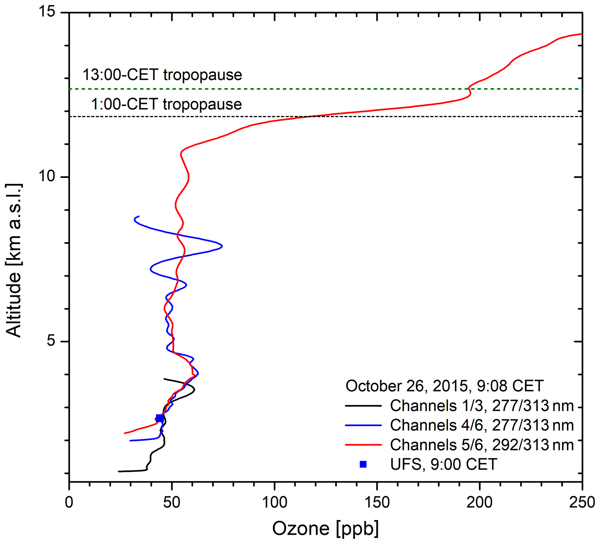
Figure 15Selection of partial ozone profiles from both receivers of the stationary system: the near-field result can be used here to more than 2 km above the lidar due to low ozone density. The ozone hump between about 3.0 and 4.8 km is caused by a remote stratospheric air intrusion. The lidar measurement agrees with that at the nearby Schneefernerhaus station (UFS, 2670 m; 0.7 ppb below blue curve). The altitude of the tropopause is taken from the Munich radiosonde.
The ozone hump between 3.0 and 4.7 km is caused by a very dry layer (1 % minimum relative humidity at 4.2 km for the Munich radiosonde, roughly 100 km to the north; 1 % is an artificial cut-off in the listings for the RS92 radiosonde; Trickl et al., 2014). 315 h backward trajectories calculated with the HYSPLIT model (Draxler and Hess, 1998; http://ready.arl.noaa.gov/HYSPLIT_traj.php, last access: 19 November 2020), selecting reanalysis meteorological data, suggest a long-range descent from the stratosphere over western Canada. The Munich thermal tropopause for both standard launch times is significantly higher than the onset of the ozone rise. It is well-known, also from our measurements, that the thermal tropopause does not perfectly coincide with the onset of the ozone rise (Hoerling et al., 1991; Pan et al., 2004).
In general, as pointed out in Sect. 4.2, the near-field receiver yields reasonable ozone typically up to at least 2 km above the ground (2.74 km a.s.l). The quality is limited due to the rapid drop of the backscatter signal. The useful range for 277 nm of the far-field receiver is 6.5 to 8 km in winter (40 to 50 ppb). 292 nm is rarely used in the lower troposphere because of the lower sensitivity for ozone and the stronger sensitivity to aerosol (Eisele and Trickl, 2005). However, the 277–292 nm profiles are preferred in the presence of pronounced aerosol structures because of a less critical aerosol correction. The typical range for 292 nm is roughly 3 km above the tropopause, which can vary with the slope of ozone rise. In summer, when ozone in the free troposphere can exceed 100 ppb, sometimes the range is limited to 10 to 11 km and the seasonally higher tropopause is not reached due to the strong loss of radiation.
Due to the short measurement time of just 41 s the reproducibility of the data can be easily verified. In Fig. 16 we show the profiles for three measurements under complex conditions (Saharan dust up to 4 km and a stratospheric air intrusion around 5.7 km) obtained within less than 3 min on 18 June 2013. The intrusion originated at 10 km or more higher the United States at least 13 d backward in time (Trickl et al., 2020). The layer descended to southern Spain and then turned north-eastward towards the Alps, slightly rising. Due to the long travel the minimum relative humidity was as high as 6 %, as measured by both our water vapour DIAL and the Munich radiosonde (Trickl et al., 2020).
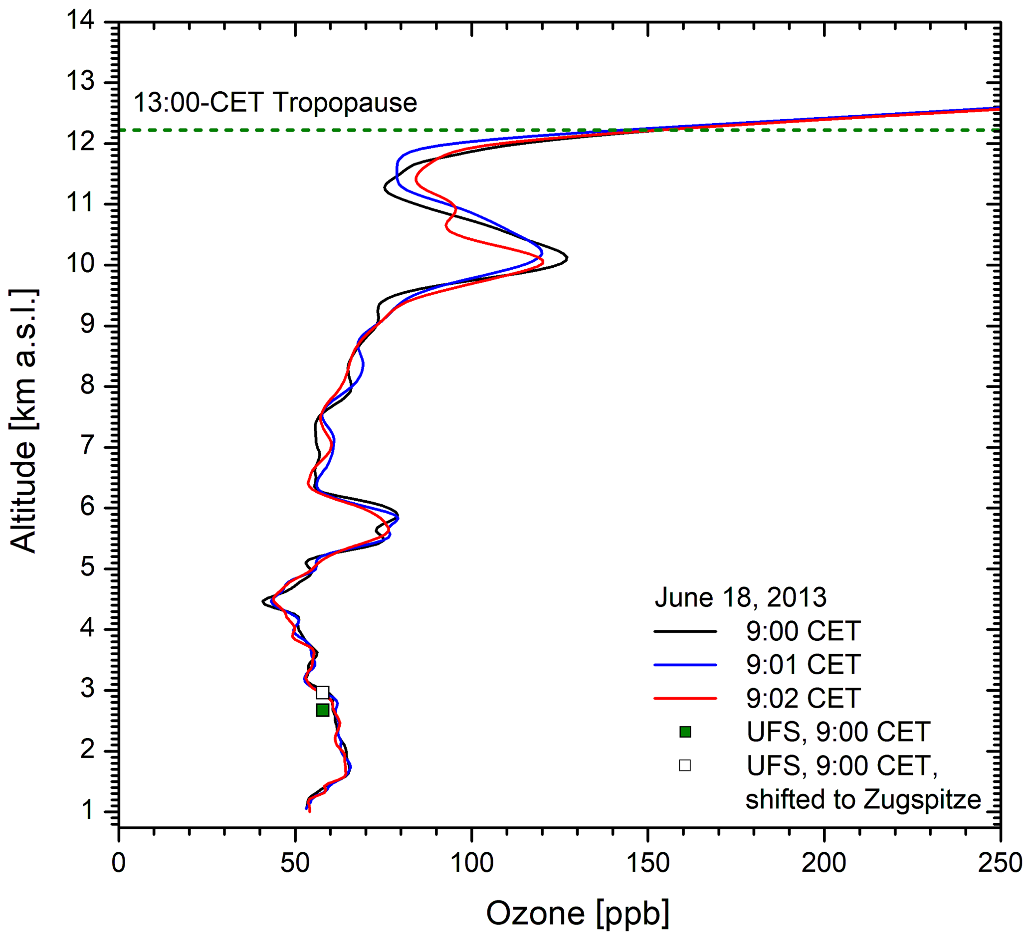
Figure 16Example for reproducibility testing during a period of elevated ozone: the on wavelengths used are 277 nm (channel 1, near-field telescope, up to 2.23 km), 277 nm (channel 6, up to about 6 km), and 292 nm (channel 5, up to the top). The lidar measurement perfectly agrees with that at UFS if the altitude is shifted to that of the Zugspitze summit (2962 m), justified by the southerly advection. Above 5 km the signal in channel 6 becomes low due to the high ozone values in the lower troposphere, and a weighted average of the 277–292 nm ozone profile with that for 292–313 nm was applied for the final few hundred metres below 6 km. Above 9 km the 292 nm signal starts to become noisy, resulting in reduced reproducibility. The altitude of the tropopause is taken from the Munich radiosonde.
Due to elevated ozone mixing ratios (50 to 80 ppb) the radiation loss results in an increase in the short-term variability of the ozone profiles in the upper troposphere, which indicates a level of uncertainty of about ±10 ppb. The noise of the 277–313 nm ozone values strongly increases above 5.5 km, where the data from the 292–313 nm pair are used.
With the latest PMT version (2012) the far-field performance of the lidar during the warm season decreases around noon due to the growing daylight background at 313 nm and the resulting nonlinearity. The 313 nm constant background is largest in the presence of clouds. The signal must be corrected mathematically (Sect. 5) to achieve both a quantitative ozone profile and a reasonable aerosol retrieval with zero aerosol in clean parts of the atmosphere. The DIAL result based on the corrected 313 nm data is then also compared with the 292 nm single-trace ozone retrieval and usually agrees well. These comparisons demonstrate the value of simultaneously evaluating aerosol and O3. For the strongest ozone mixing ratios (exceeding 100 ppb in the middle and upper troposphere) the range of the system may be limited to about 10 km and the stratospheric ozone rise is missed.
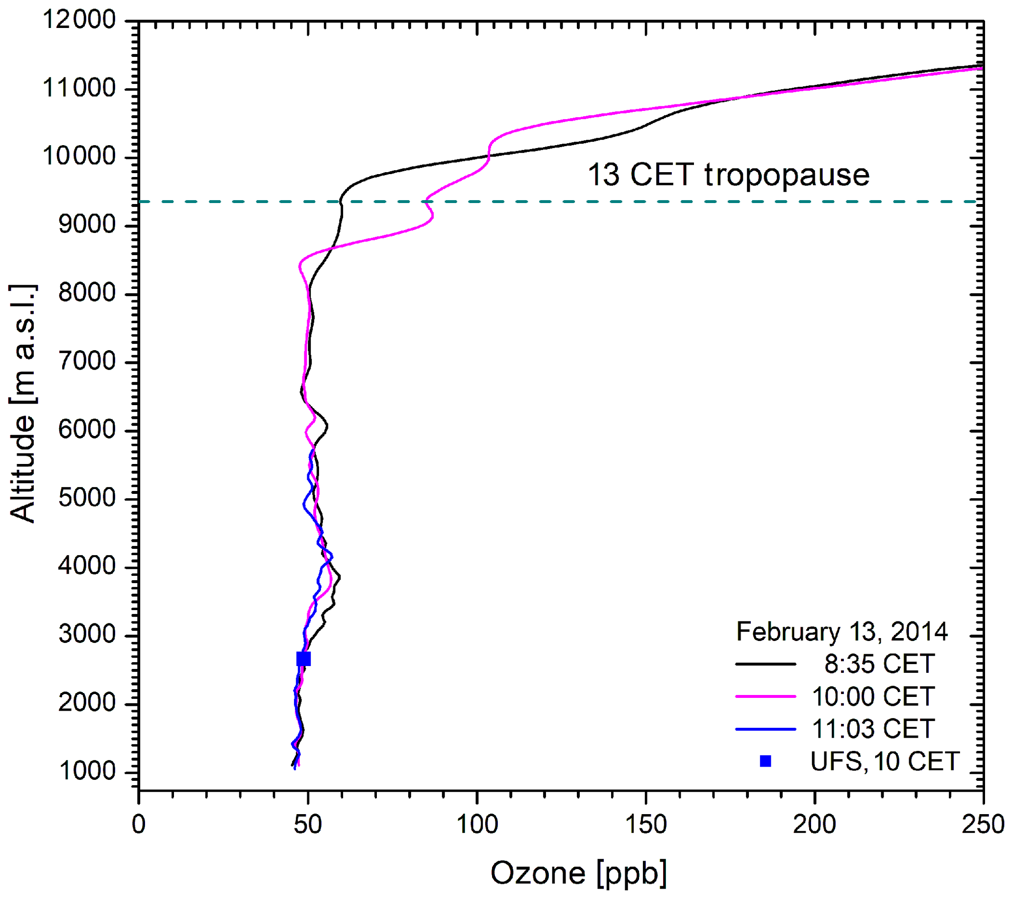
Figure 17Ozone measurement with the stationary DIAL on 13 February 2014; the variability is low apart from the two dry layers at below 4 km and at 6.1 km that are also visible in the 01:00 CET Munich radiosonde data and that seem to erode after 08:35 CET. The agreement with the in situ measurements at UFS is perfect.
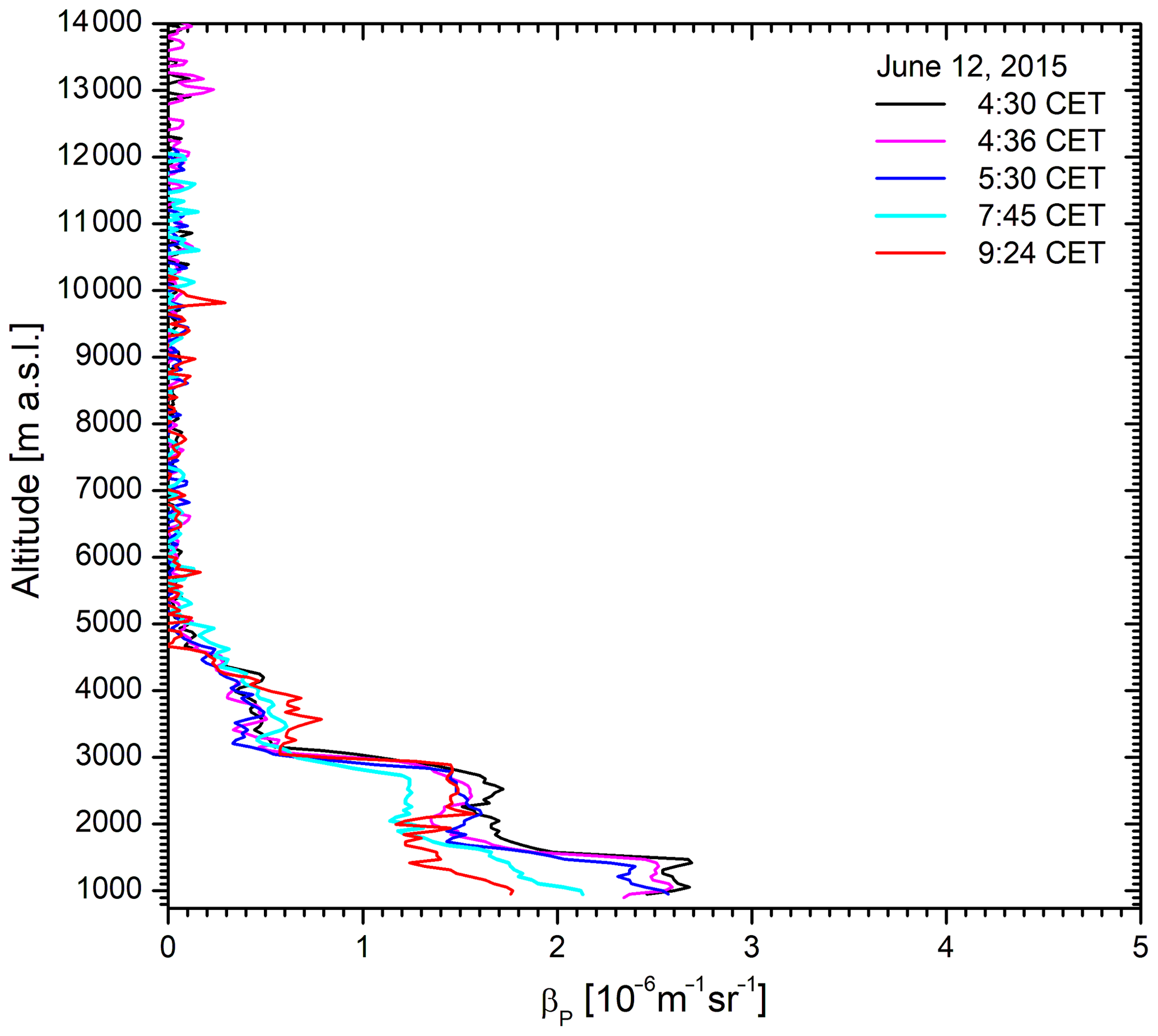
The best results are achieved in winter due to low ozone and low solar background. In Fig. 18 we give as an example the measurements on 13 February 2014. The measurements were limited to the morning hours due to the arrival of clouds ahead of a cold front, just before 11:00 CET. The profiles coincide extremely well outside two dry layers (01:00 CET Munich radiosonde, 4 % to 12 % and 6 % RH, respectively) in the lower free troposphere and above 6 km that might be associated with the slightly elevated ozone at 08:00 CET at around 3.8 and 6.1 km, respectively. The tiny peak at 6.1 km at 08:35 CET does not significantly exceed the uncertainty level in that altitude range. However, in addition to the low RH around 01:00 CET the corresponding HYSPLIT trajectories indicate a descent over at least 13 d from high altitudes over the North Pacific for both layers, confirming the idea of stratospheric intrusions. Intrusions with just a low rise in ozone are not rare during the cold season (Trickl et al., 2020). They can be resolved at least in the range covered by the less noisy 277–313 nm wavelength pair.
In Fig. 19 examples of aerosol retrievals of ozone-corrected 313 nm backscatter profiles during the brightest period of the year are shown. A constant backscatter-to-extinction ratio of 0.020 sr−1 was applied. Backscatter coefficients of (1– m−1 sr−1 are typical of the warm season at this site unless there is a strong Saharan dust or fire event. Here, the air masses originate in Italy and eastern Europe. The top altitude of 5 km resembles that for Saharan dust (Jäger et al., 1988; Papayannis et al., 2008) but was caused by orographic lifting during transport across the Alps almost parallel to the mountains. The free troposphere was free of aerosol on that day, which allows one to visualize the low noise of the lidar, at least during the early hours. Aerosol data from ultraviolet channels are usually strongly influenced by the noise of the strong Rayleigh background.
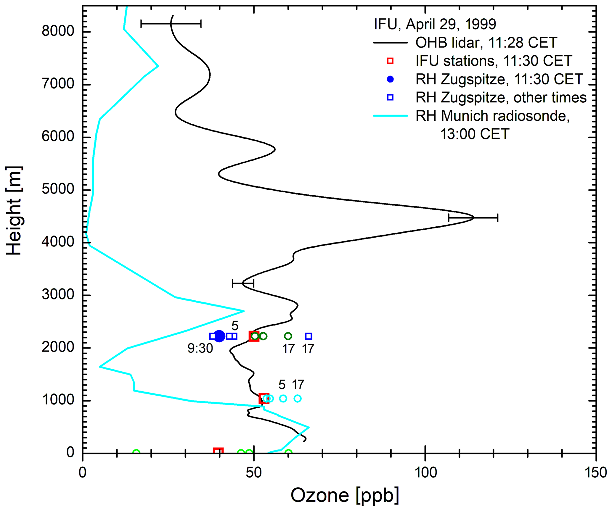
Figure 19Ozone measurement with the mobile DIAL during the brightest part of the day, after all modifications had been made (about 104 laser shots); the vertical axis is the height above the lidar site (IFU, 730 m a.s.l.), and up to 2.7 km above the ground 266–299 nm wavelength pairs were taken (near-field: up to 1.5 km). Up to 3.7 km the combination 289–299 nm was used. Above this, ozone was obtained from a single-trace evaluation for 299 nm, slightly recalibrated at the lower end of that range. For comparison, in situ ozone values from the three local monitoring stations IFU (745 m a.s.l.), Wank (1780 m a.s.l.), and Zugspitze (2962 m a.s.l.) are shown for 11:30 CET (red squares). Additional values from these stations are marked with open circles for 05:00 CET, 09:30 CET, 14:00 CET, and 17:00 CET (labelled in some cases). For the interpretation of the complicated meteorological situation, the corresponding relative humidity of the Zugspitze summit and the noon operational ascent of the Munich radiosonde are also included. Outside the most reliable part of the operating range a few representative error bars are drawn.
In the presence of strong aerosol in the planetary boundary layer (PBL), such as in the case of smoke or pronounced Saharan dust, the signal-to-noise ratio is strongly attenuated. High-aerosol events prevail in summer, which adds to lowering the upper-tropospheric performance of the system.
Starting in late 2012, the aerosol backscatter coefficients were archived in the EARLINET database, mostly with a delay of less than 1 d after the measurements.
7.2 Examples for the mobile system
7.2.1 29 April 1999
The final performance of the mobile system was achieved shortly before its destruction in late May 1999 (Fig. 19). It turned out that a daylight signal background of more than 12 mV was present in the 299 nm channel, which lead to signal distortion (Sect. 4.4). Due to inserting a 300 nm cut-off filter, bridging the gap to the 320 nm edge of the Corion filter, the 299 nm channels became linear and the planned operating range of the DIAL of 4 km could be reached. As mentioned, further range extension would be possible if a rotating attenuator could be used for 299 nm to get roughly equal maximum far-field returns for 289 and 299 nm. Below a distance r of 2.7 km, 266–299 nm pairs were taken.
In the example in Fig. 19 the range could be extended to a distance r=8.3 km (9.0 km a.s.l.) by evaluating ozone from the much stronger (less noisy) 299 nm signal alone. A slight adjustment of that partial profile had to be made based on the DIAL results for lower altitudes, which resulted in elevated uncertainties. As can be seen from the edges of the isolated structures, smoothing over several hundred metres was applied here.
The validation is based just on comparisons with the in situ measurements at the three local stations operated by IFU. The small deviations from the 11:30 CET Wank and Zugspitze in situ data also shown in the figure suggest an uncertainty of 2 ppb in this altitude range. For the higher altitudes a comparison is missing because the measurement was made on a Thursday, too early for the Friday morning Hohenpeißenberg ozonesonde ascent.
As can be concluded from the rich structure of the ozone profile and the pronounced ozone changes in the in situ data (in Fig. 19 we select the data for 05:00, 09:30, 11:30, 14:00, and 17:00 CET), the meteorological situation was complex. The situation was characterized by prefrontal advection of North American air via Algeria at most altitudes, where the minimum altitude of about 1.5 km was reached. Up to r=3.5 km the ozone profile is difficult to interpret. The ozone peak between 2.5 and 3.0 km is not necessarily caused by a subsiding stratospheric air intrusion: the relative humidity (RH) at the Zugspitze summit rose from 38 % to 66 % until 17:00 CET, when the Zugspitze ozone reached the mixing ratio of the 11:30 peak above the summit. Subsidence is not very likely under prefrontal conditions anyway (Trickl et al., 2020). Also, contributions from northern Italy could have been picked up.
Above 3.5 km we clearly see a pronounced stratospheric intrusion layer. This view is supported by the very high peak ozone of 113 ppb, the minimum RH of 1 % in the 13:00 CET ascent of the Munich radiosonde, and HYSPLIT backward trajectories. The HYSPLIT trajectories revealed descent over more than 10 d from the north-western part of North America or beyond.
The low upper-tropospheric ozone values are in agreement with the calculated source region 2 km above the Pacific south of Hawaii. Directly above the remote Pacific almost zero ozone has been found (Kley et al., 1996), which justifies the assumption of 20–30 ppb 2 km above the surface.
7.2.2 Milano field campaign
The second example is chosen from the VOTALP II (Vertical Ozone Transport in the Alps) Milano field campaign in 1998, in a joint effort together with the PIPAPO (Pianura Padana Produzione di Ozono) air-quality campaign around Milano (Italy) (more details on the measurements: Trickl, 2010b). The mobile ozone DIAL was operated at Barni (Provincia di Como) within the first mountain range of the Alps, about 40 km north of Milano between 1 and 5 June 1998. On the first 4 d a day-by-day increase in the afternoon peak ozone advected from the Milano metropolitan area to Barni by the daytime up-valley wind was observed. During each night the O3 mixing ratio dropped to roughly 60 ppb due to the reversal of the orographic wind direction.
Figure 20 shows the situation for the day with the highest ozone values, 4 June. The behaviour of the ozone rise was surprisingly similar to that on the previous days, including the bimodal profile at 13:36 CET (Central European Time = UTC +1 h). In the late afternoon 120 ppb of ozone was reached, exactly verified by side-by-side measurements with ozonesondes launched by a team from the Swiss Paul-Scherrer Institute. This high mixing ratio turned out to be the very limit for retaining an overlap between the near-field and the far-field 266 nm “on” detection channels for the chosen position of the far-field apertures (blades) and PMT settings. The comparison of the DIAL and the sonde measurements also indicates some air-mass lifting towards the main part of the lake since the boundary layer height (defined here by elevated ozone) grew as the sonde drifted northward during its ascent. It is interesting to note that the 19:10 CET DIAL profile next to the ground would agree with the sonde profiles for some average position of the two sonde maxima.
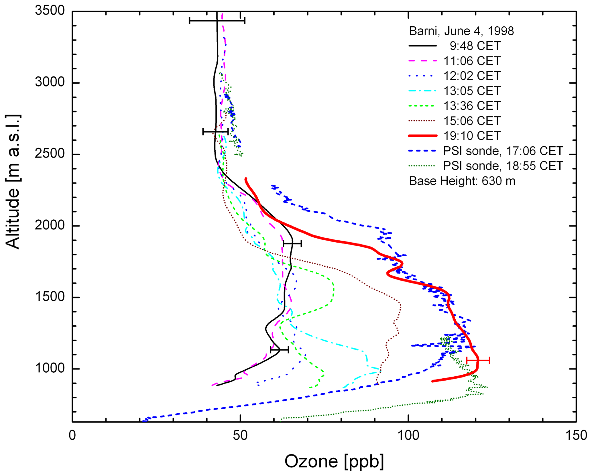
Figure 20Ozone measurements at Barni (Provincia di Como, Italy) on 4 June 1998 during the VOTALP Milano field campaign; the profiles show the daytime gradual advection of the Milano ozone plume. The ozonesonde data from the two launches at the lidar site have been kindly supplied by J. Keller (Paul-Scherrer-Institut, Switzerland; the times are launch times). Only 266 nm could be used as the on wavelength. As a consequence the range was strongly reduced during the period with the highest ozone mixing ratio.
Differential-absorption lidar systems for trace-gas measurements have proved to be an invaluable tool for atmospheric studies (Trickl, 2010b). Despite this fact the application of DIAL systems is rather limited, in particular combined approaches. Despite promising developments in Europe within TESLAS in the early 1990s no continental-scale ozone lidar network could be established. Ozone measurements have been mostly limited to Haute Provence (Gaudel et al., 2015; Tarasick et al., 2019), Garmisch-Partenkirchen, and Athens (Kalobakas et al., 2012; Mytilinaios et al., 2018). By contrast, the ozone lidar network TolNET was implemented in North America (Newchurch et al., 2016).
At IMK-IFU (Garmisch-Partenkirchen, Germany) three DIAL systems have been developed since 1988, two for ozone and one for water vapour (Vogelmann and Trickl, 2008). The ozone systems were used for a large number of focused investigations until 2003 (e.g. Carnuth et al., 2002; Eisele et al., 1999; Stohl and Trickl, 1999; Trickl, 2003; Trickl et al., 2003, 2010, 2011). The stationary ozone and water vapour lidars have been used for routine measurements since 2007 (e.g. Trickl et al., 2014, 2015, 2016, 2020). The measurements with the stationary ozone DIAL have yielded a total of almost 5000 evaluated ozone profiles since 1991. In the absence of interruptions in the measurement programme, the typical annual number of evaluated measurements has been of the order of 500. This number will grow with further increasing reliability of the automatically produced quick-look ozone and 313 nm aerosol profiles due to a diminishing requirement for manual optimization. Manual corrections are still required in the presence of high ozone levels due to the residual daytime issues at 313 nm and in the presence of pronounced aerosol and cloud structures.
In the course of 3 decades of ozone DIAL development at IMK-IFU we have gradually optimized the technology to a state in which even small variations in tropospheric ozone can be sensed with a high level of credibility. A full restriction to analogue data acquisition is possible due to the large dynamic range of the 5600 and 7400 Hamamatsu PMTs. Automatic operation was introduced in 1996 (for both systems), although it has been limited to clear-weather situations. Thus, the largest effort has been devoted to data evaluation. The results of automatic data evaluation have rarely been directly adopted and careful manual corrections have been made. These corrections include the selection of the best partial profiles based on comparisons and optimizing the vertical resolution in relation to the changing signal-to-noise ratio or when zooming into interesting ozone features. As a consequence of the excellent data quality the full use of automatic data evaluation is now coming within reach, at least under conditions of low to moderate aerosol.
The quality of the retrieved 313 nm aerosol backscatter coefficients almost matches that traditionally obtained in the green spectral region. Baseline corrections are needed during daytime due to signal distortions caused by the high daylight sensitivity of the 7400 PMTs. Spectral filtering must be improved. Perhaps one of the old 5400 PMTs must return to the far-field 313 nm channel.
Quite a number of lessons have been learnt.
-
Three-wavelength operation is mandatory: it provides a wide vertical range and internal quality assurance; the aerosol retrieval yields an additional quality control of the 313 nm backscatter profiles.
-
Use of at least one short on wavelength below 280 nm is an important base for high accuracy and for a low to moderate level of interference by aerosols that can be readily corrected for. Even for 266 nm a range up to about r=2.5 km above the lidar was demonstrated.
-
A short measurement time of 41 s was achieved with the stationary system, whereas for the mobile system about 10 min were necessary. This longer signal accumulation is in part due to the slower repetition rate of 15 Hz per wavelength for the longer wavelengths and also in part to the strong signal decay for 266 nm (30 Hz repetition rate) that necessitates longer averaging to achieve a reasonable signal-to-noise ratio at larger distances. For the stationary system, longer averaging (e.g. 5 min) will yield better results in the upper troposphere in summer. In principle, the free-tropospheric capability (i.e. without significant amounts of aerosol) can be driven close to the uncertainty limit set by the absorption cross sections.
-
Current-day transient digitizers make single-photon counting in an ozone DIAL almost superfluous, except for very long measurements in a dark environment.
-
Simultaneous analogue and PC counting out of a single PMT is possible but has so far led to a deterioration of the analogue signal that cannot easily be corrected mathematically (see Klanner et al., 2020). Single-photon counting will be resumed if the residual signal distortions can be removed. However, an operation for low PMT supply voltages must be ensured to avoid signal attenuation and excessively long averaging.
-
The application of the small Hamamatsu PMTs has allowed the use of higher signal voltage levels (100 mV or more) than in the traditionally used phototubes. A photon flux as high as possible should be applied in the far-field channels since the signal noise is strongly influenced by the photon noise1. This is an issue if both analogue and photon counting from the same PMT are chosen because photon counting requires elevated supply voltages of the order of 800 V, too high for strong irradiation.
-
A problem with the Hamamatsu 7400 PMTs not yet fully solved is the high sensitivity with respect to daylight: the background signal must not exceed 1 mV in order to avoid undershot, which can be minimized by higher laser pulse energy (improving the peak-signal-to-background ratio), careful spectral filtering, reducing the slit width at the polychromator entrance, adding another black baffle for the incoming radiation just below the entrance flap in the roof, and a very clean surface of the primary mirror of the telescope. Also, for 313 nm, a return to a 5600 PMT can be considered in the far-field receiver.
-
The use of two spatially separated telescopes for near-field–far-field separation is superior to cutting off the near-field portions in the far-field channels as done in the mobile system (and the water vapour DIAL; Vogelmann and Trickl, 2008), unless a rotating signal attenuator is used for reducing the stronger off return.
-
An operational calculation of uncertainties is planned, an important requirement for archiving data in international databases.
Table A1List of citations for atmospheric transport studies including ozone lidar systems.
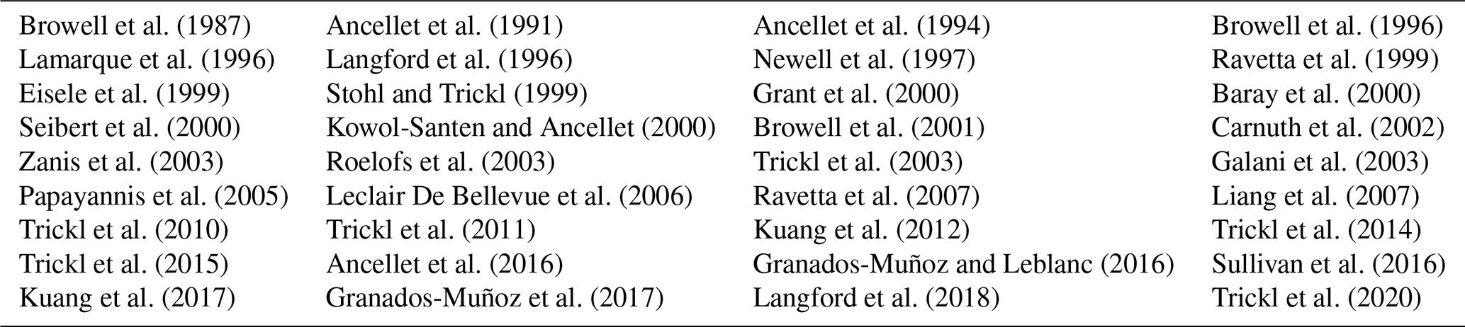
Table A2List of citations for air-quality studies including ozone lidar systems.
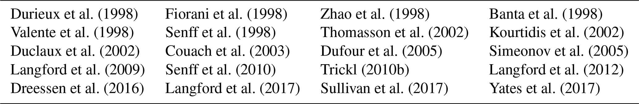
Table A3List of citations for papers describing ozone DIAL systems.
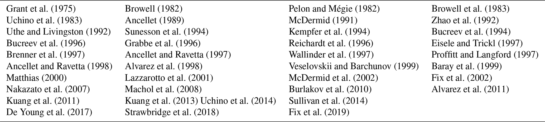
Data and information on the lidar systems can be obtained on request from the corresponding author of this paper (thomas@trickl.de as of February 2020). The 313 nm aerosol backscatter coefficients are archived in the EARLINET database, which is accessible through the ACTRIS data portal at http://actris.nilu.no/ (last access: 19 November 2020, ACTRIS, 2020).
TT carried out most lidar measurements after spring 1997, following U. Kempfer and H. Eisele, assisted by HG and MP. He has led the technical development of both ozone DIAL systems since 1990. FN was responsible for the technical infrastructure of the mobile system. HG, MP, and HV have been involved in the system upgrading since 2007.
The authors declare that they have no conflict of interest.
The authors thank Wolfgang Seiler and Hans Peter Schmid for their support over many years. Walter Carnuth designed the first version of the stationary ozone DIAL that was built by Ulrich Kempfer and Raul Lotz. The decisive upgrading, which included a lot of new approaches, was achieved in cooperation with Holger Eisele. The authors are indebted to Werner Funk, Bernd Mielke, Heinz Josef Romanski, and Bernhard Stein for numerous important discussions and technical improvements of the detection electronics. The valuable contributions during certain periods of the system development by Pietro Brenner, Josef-Michael Burger, Bernd Jänker, and Karl Maurer are emphasized. Hans-Eckhart Scheel, Ludwig Ries, Hans Claude, and Wolfgang Steinbrecht have provided reference ozone data for the Wank, Zugspitze, and Schneefernerhaus mountain stations in the vicinity of IFU and ozonesonde data for the Hohenpeißenberg observatory of the German weather service. Johannes Keller provided the ozonesonde profiles of the team from the Swiss Paul-Scherrer-Institut for the Milano field campaign. The development of the mobile system was based on a highly efficient cooperation with the company OHB System (Bremen). The different steps of the lidar development have been funded by the German Ministry of Research and Technology (BMFT), the German Foundation for the Environment (DBU, two projects), and the Bavarian Ministry of Economics. Since 2007 the aerosol results have contributed to EARLINET (European Aerosol Research Lidar Network), which is currently part of the European Research Infrastructure ACTRIS.
The article processing charges for this open-access publication were covered by a Research Centre of the Helmholtz Association.
This paper was edited by Mark Weber and reviewed by two anonymous referees.
ACTRIS: Data Policy Disclaimer, available at: http://actris.nilu.no/, last access: 19 November 2020.
Amodeo, A., Bösenberg, J., Ansmann, A., Balis, D., Böckmann, C., Chaikovsky, A., Comeron, A., Mitev, V., Papayannis, A., Pappalardo, G., Perrone, M. R., Rizi, V., Simeonov, V., Sobolewski, P., Spinelli, N., Stoyanov, D. V., Trickl, T., and Wiegner, M.: EARLINET: the European Aerosol Lidar Network, Optica Pura y Aplicada, 39, 1–10, 2006.
Ancellet, A. and Ravetta, F.: The Airborne Lidar for Tropospheric Ozone (ALTO), Advances in Atmospheric Remote Sensing with Lidar in Selected Papers of the 18th International Laser Radar Conference, Berlin (Germany, 1996), edited by: Ansmann, A., Neuber, R., Rairoux, P., and Wandinger, U., Springer, Berlin, Heidelberg, New York, 22–26 July 1996, 399–402, 1997.
Ancellet, A. and Ravetta, F.: Compact airborne lidar for tropospheric ozone: description and field measurements, Appl. Opt., 37, 5509–5521, 1998.
Ancellet, G., Papayannis, A., Pelon, J., and Mégie, G.: DIAL Tropospheric Ozone Measurement Using a Nd:YAG Laser and the Raman Shifting Technique, J. Atmos. Oceanic Technol., 6, 832–839, 1989.
Ancellet, G., Pelon, J., Beekmann, M., Papayannis, A., and Mégie, G.: Ground-Based Lidar Studies of Ozone Exchanges Between the Stratosphere and the Troposphere, J. Geophys. Res., 96, 22401–22421, 1991.
Ancellet, A., Beekmann, M., and Papayannis, A.: Impact of cutoff low development on downward transport of ozone in the troposphere, J. Geophys. Res., 99, 3451–3468, 1994.
Ancellet, G., Pelon, J., Totems, J., Chazette, P., Bazureau, A., Sicard, M., Di Iorio, T., Dulac, F., and Mallet, M.: Long-range transport and mixing of aerosol sources during the 2013 North American biomass burning episode: analysis of multiple lidar observations in the western Mediterranean basin, Atmos. Chem. Phys., 16, 4725–4742, https://doi.org/10.5194/acp-16-4725-2016, 2016.
Alvarez II, R. J., Senff, C. J., Hardesty, R. M., Parrish, D. D., Like, W. T., Watson, T. B., Daum, P. H., and Gillani, N.: Comparisons of airborne lidar measurements of ozone with airborne in situ measurements during the 1995 Southern Oxidants Study, J. Geophs. Res., 103, 31155–31171, 1998.
Alvarez II, R. J., Senff, C. J., Langford, A. O., Weikmann, A. M., Law, D. C., Machol, J. L., Merrit, D. A., Marchbanks, R. D., Sandberg, S. P., Brewer, W. A., Hardesty, R. M., and Banta, R. M.: Development and application of a compact, tunable, solid-state airborne ozone lidar system for boundary layer profiling, J. Atmos. Ocean. Technol., 28, 1258–1271, 2011.
ATMOFAST: Atmosphärischer Ferntransport und seine Auswirkungen auf die Spurengaskonzentrationen in der freien Troposphäre über Mitteleuropa (Atmospheric Long-range Transport and its Impact on the Trace-gas Composition of the Free Troposphere over Central Europe), Project Final Report, T. Trickl, co-ordinator, M. Kerschgens, A. Stohl, and T. Trickl, subproject co-ordinators, funded by the German Ministry of Education and Research within the programme “Atmosphärenforschung 2000“, Forschungszentrum Karlsruhe, IMK-IFU (Garmisch-Partenkirchen, Germany), http://www.trickl.de/ATMOFAST.htm (last access: 19 November 2020), 130 pp., 2005 (with revised publication list 2012; in German).
Banta, R. M., Senff, C. J., White, A. B., Trainer, M., McNider, R. T., Valente, R. J., Mayor, S. D., Alvarez, R. J., Hardesty, R. M., Parrish, D., and Fehsenfeld, F. C.: Daytime buildup and nightime transport of urban ozone in the boundary layer during a stagnation episode, J. Geophys. Res., 103, 22519–22544, 1998.
Baray, J.-L., Leveau, J., Porteneuve, J., Ancellet, G., Keckhut, P., Posny, F., and Baldy, S.: Description and and evaluation of a tropospheric ozone lidar implemented on an existing lidar in the southern subtropics, Appl. Opt., 38, 6808–6817, 1999.
Baray, J.-L., Daniel, V., Ancellet, G., and Legras, B.: Planetary-scale tropopause folds in the southern subtropics, Geophys. Res. Lett., 27, 353–356, 2000.
Blackman, R. B. and Tukey, J. W.: in: The Measurement of Power Spectra, From the Point of View of Communications Engineering, Dover, Publications, New York, USA, 95–101, 1959.
Bragg, S. L., Brault, J. W., and Smith, W. H.: Line Positions and Strengths in the H2 Quadrupole Spectrum, Astrophys. J., 263, 999–1004, 1982.
Brenner, P., Reitebuch, O., Schäfer, K., Trickl, T., and Stichternath, A.: A Novel Mobile Vertical-sounding System for Ozone Studies in the Lower Troposphere”, Advances in Atmospheric Remote Sensing with Lidar, Selected Papers of the 18th International Laser Radar Conference, Berlin (Germany, 1996), edited by: Ansmann, A., Neuber, R., Rairoux, P., and Wandinger, U., Springer, Berlin, Heidelberg, New York, 22–26 July 1996, 383–386, 1997.
Browell, E. V.: Lidar measurements of tropospheric gases, Opt. Eng., 21, 128–132, 1982.
Browell, E. V., Carter, A. F., Shipley, S. T., Allen, R. J., Butler, C. F., Mayo, M. N., Siviter, J. H., and Hall, W. M.: NASA multipurpose airborne DIAL system and measurements of ozone and aerosol profiles, Appl. Opt., 22, 522–534, 1983.
Browell, E. V., Danielsen, E. F., Ismail, S., Gregory, G. L., and Beck, S. M.: Tropopause Fold Structure Determined From Airborne Lidar and in Situ Measurements, J. Geophys. Res., 92, 2112–2120, 1987.
Browell, E. V., Fenn, M. A., Butler, C. F., Grant, W. B., Merrill, J. T., Newell, R. E., Bradshaw, J. D., Sandholm, S. T., Anderson, B. E., Bandy, A. R., Bachmeier, A. S., Blake, D. R., Davis, D. D., Gregory, G. L., Heikes, B. G., Kondo, Y., Liu, S. C., Rowland, F. S., Sachse, G. W., Singh, H. B., Talbot, R. W., and Thornton, D. C.: Large-scale air mass characteristics observed over the Western Pacific during summertime, J. Geophys. Res., 111, 1691–1712, 1996.
Browell, E. V., Fenn, M. A., Butler, C. F., Grant, W. B., Ismail, S., Ferrare, R. A., Kooi, S. A., Brackett, V. G., Clayton, M. B., Avery, M. A., Barrick, J. D. W., Fuelberg, H. E., Maloney, J. C., Newell, R. E., Zhu, Y., Mahoney, M. J., Anderson, B. E., Blake, D. R., Brune, W. H., Heikes, B. G., Sachse, G. W., Singh, H. B., and Talbot, R. W.: Large-scale air mass characteristics observed over the remote tropical Pacific Ocean during March–April 1999: Results from the PEM-Tropics B field experiment, J. Geophys. Res., 106, 32481–32501, 2001.
Bucreev, V. S., Vartapetov, S. K., Veselovskii, I. A., Galustov, A. S., Kovalev, Y. M., Prokhorov, A. M., Svetogorov, E. S., Khmelevtsov, S. S., and Lee, C. H.: Excimer-laser-based lidar system for stratospheric and tropospheric ozone measurements, Quantum Electron+., 24, 546–551 (translated from Kvantovaya Electron+., 21, 591–596, 1994), 1994.
Bucreev, V. S., Vartapetov, S. K., Veselovskii, I. A., Galustov, A. S., Kovalev, Y. M., Svetogorov, E. S., and Khmelevtsov, S. S.: Combined lidar system for stratospheric and tropospheric ozone measurements, Appl. Phys. B, 62, 97–101, 1996.
Burlakov, V. D., Dolgii, S. I., Makeev, A. P., Nevzorov, A. V., Romanovskii, O. A., and Kharchenko, O. V.: A Differential-Absorption Lidar for Ozone Sensing in the Upper Atmosphere – Lower Stratosphere, Instrum. exp. Tech+., 53, 886–889, 2010.
Carnuth, W. and Trickl, T., Transport studies with the IFU three-wavelength aerosol lidar during the VOTALP Mesolcina experiment, Atmos. Environ., 34, 1425–1434, 2000.
Carnuth, W., Kempfer, U., and Trickl, T.: Highlights of the tropospheric lidar studies at IFU within the TOR project, Tellus B, 54, 163–185, 2002.
Couach, O., Balin, I., Jiménez, R., Ristori, P., Perego, S., Kirchner, F., Simeonov, V., Calpini, B., and van den Bergh, H.: An investigation of ozone and planetary boundary layer dynamics over the complex topography of Grenoble combining measurements and modeling, Atmos. Chem. Phys., 3, 549–562, https://doi.org/10.5194/acp-3-549-2003, 2003.
Cristofanelli, P., Bonasoni, P., Collins, W., Feichter, J., Forster, C., James, P., Kentarchos, A., Kubik, P. W., Land, C., Meloen, J., Roelofs, G. J., Siegmund, P., Sprenger, M., Schnabel, C., Stohl, A., Tobler, L., Tositti, L., Trickl, T., and Zanis, P.: Stratosphere to troposphere transport: a model and method evaluation, J. Geophys. Res., 108, 8525, https://doi.org/10.1029/2002JD002600, 2003.
Daumont, D., Brion, J., Charbonnier, J., and Malicet, J.: Ozone UV Spectroscopy I: Absorption Cross-Sections at Room Temperature, J. Atmos. Chem., 15, 145–155, 1992.
De Schoulepnikoff, L., Mitev, V., Simeonov, V., Calpini, B., and van den Bergh, H.: Experimental investigation of high-power single-pass Raman shifters in the ultraviolet with Nd:YAG and KrF lasers, Appl. Opt., 36, 5026–5043, 1997.
De Young, R., Carrion, W., Ganoe, R., Pliutau, D., Gronoff, G., Berkoff, T., and Kuang, S.: Langley mobile ozone lidar: ozone and aerosol atmospheric profiling for air quality research, Appl. Opt., 56, 721–730, 2017.
Dickensen, G. D., Niu, M. L., Salumbides, E. J., Komasa, J., Eikema, K. S. E., Pachuki, K., and Ubachs, W.: Fundamental Vibration of Molecular Hydrogen, Phys. Rev. Lett., 110, 193601, https://doi.org/10.1103/PhysRevLett.110.193601 , 2013.
Draxler, R. and Hess, G.: An overview of the HYSPLIT_4 modelling system for trajectories, dispersion, and deposition, Aust. Meteorol. Mag., 47, 295–308, 1998.
Dreessen, J., Sullivan, J., and Delgado, R.: Observations and impacts of transported Canadian wildfire smoke on ozone and aerosol air quality in the Maryland region on June 9–12, 2015, J. Air Waste Manage Assoc., 66, 842–862, 2016.
Duclaux, O., Frejafon, E., Thomasson, A., Yu, J., C., Puel, C., Savoie, F., Ritter, P., Boch, J. P., and Wolf, J. P.: 3D-air quality model evaluation using the Lidar technique, Atmos. Environ., 36, 5081–5095, 2002.
Dufour, A., Amodei, M., Ancellet, G., and Peuch, V.-H.: Observed and modelled ”chemical weather” during ESCOMPTE, Atmos. Res., 74, 161–189, 2005.
Durieux, E., Fiorani, L., Calpini, B., Flamm, M., Jaquet, L., and van den Bergh, H.: Tropospheric Ozone Measurements over the Great Athens Area during the MEDCAPHOT-TRACE Campaign, Atmos. Environ., 32, 2141–2150, 1998.
Eisele, H.: Aufbau und Betrieb eines Dreiwellenlängen-Lidars für Ozonmessungen in der gesamten Troposphäre und Entwicklung eines neuen Auswerteverfahrens zur Aerosol-korrektur, Dissertation, Universität Tübingen (Germany, 1997), published as Schriftenreihe des Fraunhofer-Instituts für Atmosphärische Umweltforschung, Vol. 55, Verlag Dr. W. Maraun, Frankfurt/Main, Germany, 1998, ISBN 3-932666-08-9, 107 pp., 1997 (in German).
Eisele, H. and Trickl, T.: Second Generation of the IFU Stationary Tropospheric Ozone Lidar, Advances in Atmospheric Remote Sensing with Lidar, Selected Papers of the 18th International Laser Radar Conference (Berlin, Germany, 1996), edited by: Ansmann, A., Neuber, R., Rairoux, P., and Wandinger, U., Springer, Berlin, Heidelberg, New York, 22–26 July 1996, 379–382, 1997.
Eisele, H. and Trickl, T.: Improvements of the aerosol algorithm in ozone-lidar data processing by use of evolutionary strategies, Appl. Opt., 44, 2638–2651, 2005.
Eisele, H., Scheel, H. E., Sladkovic, R., and Trickl, T.: High-Resolution Lidar Measurements of Stratosphere-Troposphere Exchange, J. Atmos. Sci., 56, 319–330, 1999.
EUROTRAC: Transport and Chemical Transformation of Pollutants in the Troposphere, Vol. 1, An Overview of the Work of EUROTRAC, edited by: Borrell, P. and Borrell, P. M., Springer (Berlin, Heidelberg, New York), ISBN 3-540-66775-X, 474 pp., 1997.
Fiorani, L., Calpini, B., Jaquet, L., van den Bergh, H., and Durieux, E.: A Combined Determination of Wind Velocities and Ozone Concentration for a First Measurement of Ozone Fluxes with a DIAL Instrument during the MEDCAPHOT-TRACE Campaign, Atmos. Environ., 32, 2151–2159, 1998.
Fix, A., Wirth, M., Meister, A., Ehret, G., Pesch, M., and Weidauer, D.: Tunable ultraviolet optical parametric oscillator for differential absorption lidar measurements of tropospheric ozone, Appl. Phys. B., 75, 153–163, 2002.
Fix, A., Steinebach, F., Wirth, M., Schäfler, A., and Ehret, G.: Development and application of an airborne differential absorption lidar for the simultaneous measurement of ozone and water vapor profiles in the tropopause region, Appl. Opt., 58, 5892–5900, 2019.
Freudenthaler, V.: The telecover test: A Quality assurance tool for the optical part of a lidar system, in: Reviewed and Revised Papers Presented at the 24th International Laser Radar Conference, Boulder, Colorado, USA, 23–27 June 2008, Vol. II, edited by: Hardesty, M. and Mayor, S., ISBN 978-0-615-21489-4, 145–146, 2008.
Galani, E., Balis, D., Zanis, P., Zerefos, C., Papayannis, A., Wernli, H., and Gerasopoulos, E.: Observations of stratosphere-to-troposphere transport events over the eastern Mediterranean using a ground-based lidar system, J. Geophys. Res., 108, 8527, https://doi.org/10.1029/2002JD002596, 2003.
Gaudel A., Ancellet G., and Godin-Beekmann S.: Analysis of 20 years of tropospheric ozone vertical profiles by lidar and ECC at Observatoire de Haute Provence (OHP) at 44∘ N, 6.7∘ E, Atmos. Environ., 113, 78–89, 2015.
Giehl, H. and Trickl, T.: Testing the IFU High-Spectral-Resolution Lidar at the 2009 Leipzig Field Campaign, in: Proceedings of the 25th International Laser Radar Conference, St.-Petersburg (Russia), 5–9 July 2010, 2010, edited by: Matvienko, G. and Zemlyanov, A., V. E. Zuev Institute of Optics (Tomsk, Russia), 920–923, 2010.
Gorshelev, V., Serdyuchenko, A., Weber, M., Chehade, W., and Burrows, J. P.: High spectral resolution ozone absorption cross-sections – Part 1: Measurements, data analysis and comparison with previous measurements around 293 K, Atmos. Meas. Tech., 7, 609–624, https://doi.org/10.5194/amt-7-609-2014, 2014.
Grabbe, G. C., Bösenberg, J., Dier, H., Görsdorf, U., Matthias, V., Peters, G., Schaberl, T., and Senff, C.: Intercomparison of Ozone Measurements between Lidar and ECC Sondes, Contr. Atmos. Phys., 69, 189–203, 1996.
Granados-Muñoz, M. J. and Leblanc, T.: Tropospheric ozone seasonal and long-term variability as seen by lidar and surface measurements at the JPL-Table Mountain Facility, California, Atmos. Chem. Phys., 16, 9299–9319, https://doi.org/10.5194/acp-16-9299-2016, 2016.
Granados-Muñoz, M. J., Johnson, M. S., and Leblanc, T.: Influence of the North American monsoon on Southern California tropospheric ozone levels during summer in 2013 and 2014, Geophys. Res. Lett., 44, 6431–6439, https://doi.org/10.1002/2017GL073375, 2017.
Grant, W. B. and Hake, R. D.: Calibrated remote measurements of SO2 and O3 using atmospheric backscatter, J. Appl. Phys., 46, 3019–3023, 1975.
Grant, W. B., Browell, E. V., Butler, C. F., Fenn, M. A., Clayton, M. B., Hannan, J. R., Fuelberg, H. E., Blake, D. R., Blake, N. J., Gregory, G. L, Heikes, B. G., Sachse, G. W., Singh, H. B., Snow, J., and Talbot, R. W.: A case study of transport of tropical marine boundary layer and lower tropospheric air masses to the northern midlatitude upper troposphere, J. Geophys. Res., 105, 3757–3769, 2000.
Hoerling, M. P., Schaack, T. K., and Lenzen, A. J.: Global Objective Tropopause Analysis, Mon. Weather Rev., 119, 1816–1831, 1991.
Iarlori, M., Madonna, F., Rizi, V., Trickl, T., and Amodeo, A.: Effective resolution concepts for lidar observations, Atmos. Meas. Tech., 8, 5157–5176, https://doi.org/10.5194/amt-8-5157-2015, 2015.
Jäger, H., Carnuth, W., and Georgii, B.: Observations of Saharan dust at a North Alpine mountain station, J. Aerosol Sci., 19, 1235–1238, 1988.
Jennings, D. E., Weber, A., and Brault, J. W.: Raman spectroscopy of gases with a Fourier transform spectrometer: the spectrum of D2, Appl. Opt., 25, 284-290, 1986
Jeunouvrier, A., Mérienne, M.-F., Coquart, B., Carleer, M., Fally, S., Vandaele, A. C., Hermans, C., and Colin, R.: Fourier Transform Spectroscopy of the O2 Herzberg Bands – I. Rotational Analysis, J. Mol. Spectrosc., 198, 136–162, 1999.
Jonson, J. E., Simpson, D., Fagerli, H., and Solberg, S.: Can we explain the trends in European ozone levels?, Atmos. Chem. Phys., 6, 51–66, https://doi.org/10.5194/acp-6-51-2006, 2006.
Kalabokas, P., Papayannis, A., Tsaknakis, G., and Ziomas, I.: A study on the atmospheric concentrations of primary and secondary air pollutants in the Athens basin performed by DOAS and DIAL measuring techniques, Sci. Total Environ., 414, 556–563, 2012.
Kempfer, U.: Entwicklung und Anwendung eines differentiellen Absorptions-LIDAR-Systems zur Messung der troposphärischen Ozonkonzentration, Dissertation, Ludwig-Maximilians-Universität München (Germany), 151 pp., 1992.
Kempfer, U., Carnuth, W., Lotz, R., and Trickl, T.: A wide range ultraviolet lidar system for tropospheric ozone measurements: development and application, Rev. Sci. Instrum., 65, 3145–3164, 1994.
Klanner, L., Höveler, K., Khordakova, D., Perfahl, M., Rolf, C., Trickl, T., and Vogelmann, H.: A powerful lidar system capable of one-hour measurements of water vapour in the troposphere and the lower stratosphere as well as the temperature in the upper stratosphere and mesosphere, Atmos. Meas. Tech. Discuss., https://doi.org/10.5194/amt-2020-90, in review, 2020.
Kley, D., Crutzen, P. J., Smit, H. G. J., Vömel, H., Oltmans, S. J., Grassl, H., and Ramanathan, V.: Observations of near-zero ozone concentrations over the convective Pacific: effects of air chemistry, Science, 274, 230–233, 1996.
Kley, D., Beck, J., Grennfelt, P. I., Hov, O., and Penkett, S. A.: Tropospheric Ozone Research (TOR) A Sub-Project of EUROTRAC, J. Atmos. Chem., 28, 1–9, 1997.
Kourtidis, K., Zerefos, C., Rapsomanikis, S., Simeonov, V., Balis, D., Perros, P. E., Thompson, A. M., Witte, J., Calpini, B., Sharobiem, W. M., Papayannis, A., Mihalopoulos, N., and Drakou, R.: Regional levels of ozone in the troposphere over eastern Mediterranean, J. Geophys. Res., 107, 8140, https://doi.org/10.1029/2000JD000140, 2002.
Kowol-Santen, J. and Ancellet, G.: Mesoscale analysis of transport across the subtropical tropopause, Geophys. Res. Lett., 27, 3345–3347, 2000.
Kreipl, S.: Messung des Aerosoltransports am Alpennordrand mittels Laserradar (Lidar), Dissertation, Friedrich-Alexander-Universität Erlangen-Nürnberg (Germany), 195 pp., 2006 (in German).
Krupenie, P. H.: The Spectrum of Molecular Oxygen, J. Phys. Chem. Ref. Data, 1, 423–534, 1972.
Kuang, S., Burris, J. F., Newchurch, M. J., Johnson, S., and Long, S.: Differential Absorption Lidar to measure subhourly variation of tropospheric ozone profiles, IEEE Trans. Geosci. Remote Sens., 49, 557–571, 2011.
Kuang, S., Newchurch, M. J., Burris, J., Wang, L., Knupp, K., and Huang, G.: Stratosphere-to-troposphere transport revealed by ground-based lidar and ozonesonde at a midlatitude site, J. Geophys. Res., 117, D18305, https://doi.org/10.1029/2012JD017695, 2012.
Kuang, S., Newchurch, M. J., Burris, J. F., and Liu, X.: Ground-based lidar for atmospheric boundary layer ozone measurements, Appl. Opt., 52, 3557–3566, 2013.
Kuang, S., Newchurch, M. J., Johnson, M. S., Wang, L., Burris, J. F., Pierce, R. B., Eloranta, E. W., Pollack, I. W., Graus, M., de Gouw, J., Warneke, C., Ryerson, T. B., Markovic, M. Z., Holloway, J. S., Pour-Biazar, A., Huang, G., Liu, X., and Feng, N.: Summertime tropospheric ozone enhancement associated with a cold front passage due to stratosphere-to-troposphere transport and biomass burning: Simultaneous ground-based lidar and airborne measurements, J. Geophys. Res., 122, 1293–1311, https://doi.org/10.1002/2016JD026078, 2017.
Lamarque, J.-F., Langford, A. O., and Proffitt, M. H.: Cross-tropopause mixing of ozone through gravity wave breaking: Observation and modelling, J. Geophys. Res., 101, 22969–22976, 1996.
Langford, A. O.: Identification and correction of analog-to-digital-converter nonlinearities and their implications for differential absorption lidar measurements, Appl. Opt., 34, 8330–8340, 1995.
Langford, A. O., Masters, C. D., Proffitt, M. H., Hsie, E.-Y., and Tuck, A. F.: Ozone measurements in a tropopause fold associated with a cut-off low system, Geophys. Res. Lett., 23, 2501–2504, 1996.
Langford, A. O., Aikin, K. C., Eubank, C. S., and Williams, E. J.: Stratospheric contribution to high surface ozone in Colorado during springtime, Geophys. Res. Lett., 36, L12801, https://doi.org/10.1029/2009GL038367, 2009.
Langford, A. O., Brioude, J., Cooper, O. R., Senff, C. J., Alvarez II, R. J., Hardesty, R. M., Johnson, B. J., and Oltmans, S. J.: Stratospheric influence on surface ozone in the Los Angeles area during late spring and early summer of 2010, J. Geophys. Res., 117, D00V06, https://doi.org/10.1029/2011JD016766, 2012.
Langford, A. O., Alvarez II, R. J., Brioude, J., Fine, R., Gustin, M. S., Lin, M. Y., Marchbanks, R. D., Pierce, R. B., Sandberg, S. P., Senff, C. J., Weickmann, A. M., and Williams, E. J.: Entrainment of stratospheric air and Asian pollution by the convective boundary layer in the southwestern U.S., J. Geophys. Res., 122, 1312–1337, https://doi.org/10.1002/2016JD025987, 2017.
Langford, A. O., Alvarez II, R. J., Brioude, Evan, S., Iraci, L. T., Kirgas, G., Kuang, S., Leblanc, T., Newchurch, M. J., Pierce, R. B., Senff, C. J., and Yates, E. L.: Coordinated profiling of stratospheric intrusions and transported pollution by the Tropospheric Ozone Lidar Network (TOLNet) and NASA Alpha Jet experiment (AJAX): Observations and comparison to HYSPLIT, RAQMS, and FLEXPART, Atmos. Environ., 174, 1–14, 2018.
Lazzarotto, B., Frioud, M., Larchevêque, G., Mitev, V., Quaglia, P., Simeonov, V., Thompson, A., van den Bergh, H., and Calpini, B.: Ozone and water-vapor measurements by Raman lidar in the planetary boundary layer: error sources and field measurements, Appl. Opt., 40, 2985–2997, 2001.
Leblanc, T., Sica, R. J., van Gijsel, J. A. E., Godin-Beekmann, S., Haefele, A., Trickl, T., Payen, G., and Gabarrot, F.: Proposed standardized definitions for vertical resolution and uncertainty in the NDACC lidar ozone and temperature algorithms – Part 1: Vertical resolution, Atmos. Meas. Tech., 9, 4029–4049, https://doi.org/10.5194/amt-9-4029-2016, 2016.
Leblanc, T., Brewer, M. A., Wang, P. S., Granados-Muñoz, M. J., Strawbridge, K. B., Travis, M., Firanski, B., Sullivan, J. T., McGee, T. J., Sumnicht, G. K., Twigg, L. W., Berkoff, T. A., Carrion, W., Gronoff, G., Aknan, A., Chen, G., Alvarez, R. J., Langford, A. O., Senff, C. J., Kirgis, G., Johnson, M. S., Kuang, S., and Newchurch, M. J.: Validation of the TOLNet lidars: the Southern California Ozone Observation Project (SCOOP), Atmos. Meas. Tech., 11, 6137–6162, https://doi.org/10.5194/amt-11-6137-2018, 2018.
Leclair De Bellevue, J., Réchou, A., Baray, J. L., Ancellet, G., and Diab, R. D.: Signatures of stratosphere to troposphere transport near deep convective events in the southern subtropics, J. Geophys Res., 111, D24107, https://doi.org/10.1029/2005JD006947, 2006.
Liang, Q., Jaeglé, L., Hudman, R. C., Turquety, S., Jacob, D. J., Avery, M. A., Browell, E. V., Sachse, G. W., Blake, D. R., Brune, W., Ren, X., Cohen, R. C., Dibb, J. E., Fried, A., Fuelberg, H., Porter, M., Heikes, B. G., Huey, G., Singh, H. B., and Wennberg, P. O.: Summertime influence of Asian pollution in the free troposphere over North America, J. Geophys. Res., 112, D12S11, https://doi.org/10.1029/2006JD007919, 2007.
Machol, J. L., Marchbanks, R. D., Senff, C. J., McCarty, B. J., Eberhard, W. L., Brewer, W. A., Richter, R. A., Alvarez II, R. J., Law, D. C., Weickmann, A. M., and Sandberg, S. P.: Scanning tropospheric ozone and aerosol lidar with double-gated photomultipliers, Appl. Optics, 48, 512–524, 2008.
Malicet, J., Daumont, D., Charbonnier, J., Parisse, C., Chakir, A., and Brion, J.: Ozone UV Spectroscopy I: Absorption Cross-Sections and Temperature Dependence, J. Atmos. Chem., 21, 263–273, 1995.
Marenco, A., Thouret, V., Nédélec, P., Smit, H., Helten, M., Kley, D., Karcher, F., Simon, P., Law, K., Pyle, J., Poschmann, G., von Wrede, R., Hume, C., and Cook, T.: Measurement of ozone and water vapor by Airbus in-service aircraft: The MOZAIC airborne program, An overview, J. Geophys. Res., 103, 25631–25642, 1998.
Matthias, M.: Vertikalmessungen der Aerosolextinktion und des Ozons mit einem UV-Raman-Lidar, Dissertation, Universität Hamburg, published as Examensarbeit Nr. 80, Max-Planck-Institut für Meteorologie (Hamburg, Germany), ISSN 0938-5177, 143 pp., 2000 (in German).
McDermid, I. S., Haner, D. A., Kleiman, M. M., Walsh, T. D., and White, M. L.: Differential absorption lidar systems for tropospheric and stratospheric ozone measurements, Opt. Engin., 30, 22–30, 1991.
McDermid, I. S., Beyerle, G., Haner, D. A., and Leblanc, T.: Redesign and improved performance of the tropospheric ozone lidar at the Jet Propulsion Laboratory Table Mountain Facility, Appl. Opt., 41, 7550–7555, 2002.
Milton, M. J. T., Ancellet, G., Apituley, A., Bösenberg, J., Carnuth, W., Castagnoli, F., Trickl, T., Edner, H., Stefanutti, L., Schaberl, T., Sunesson, A., and Weitkamp, C.: Raman-shifted laser sources suitable for differential-absorption lidar measurements of ozone in the troposphere, Appl. Phys. B, 66, 105–113, 1998.
Mytilinaios, M., Papayannis, A., and Tsaknakis, G.: Lower-free tropospheric ozone DIAL measurements over Athens, Greece, EPJ Web of Conferences, 28th International Laser Radar Conference, Bucharest, Romania, 25–30 June 2017, 176, 05025, https://doi.org/10.1051/epjconf/201817605025, 2018.
Nakazato, M., Nagai, T., Sakai, T., and Hirose, Y.: Tropospheric ozone differential-absorption lidar using stimulated Raman scattering in carbon dioxide, Appl. Opt., 46, 2269–2279, 2007.
Newchurch, M. J., Kuang, S., Leblanc, T., Alvarez II, R. J., Langford, A. O., Senff, C. J., Burris, J. F., McGee, T. J., Sullivan, J. T., DeYoung, R. J., Al-Saadi, J., Johnson, M., and Pszenny, A.: TOLNet – A Tropospheric Ozone Lidar Profiling Network for Satellite Continuity and Process Studies, Proc. 27th International Laser Radar Conference, New York, USA, 2015, 5–10 July 2015, EPJ Web of Conferences, 119, 20001, 2016.
Newell, R. E., Browell, E. V., Davis, D. D., and Liu, S. C.: Western Pacific ozone and potential vorticity: Implications for Asian pollution, Geophys. Res. Lett., 24, 2733–2736, 1997.
Ordoñez, C., Brunner, D., Staehelin, J., Hadjinicolaou, P., Pyle, J. A., Jonas, M., Wernli, H., and Prévôt, A. S. H.: Strong influence of lowermost stratospheric ozone on lower tropospheric background ozone changes over Europe, Geophys. Res. Lett., 34, L07805, https://doi.org/10.1029/2006GL029113, 2007.
Pan, L. L., Randel, W. J., Gary, B. L., Mahoney, M. J., and Hintsa, E. J.: Definitions and sharpness of the extratropical tropopause: A trace gas perspective, J. Geophys. Res., 109, D23103, https://doi.org/10.1029/2004JD004982, 2004.
Papayannis, A., Ancellet, G., Pelon, J., and Mégie, G.: Multiwavelength lidar for ozone measurements in the troposphere and the lower stratosphere, Appl. Opt., 29, 467–476, 1990.
Papayannis, A., Balis, D., Zanis, P., Galani, E., Wernli, H., Zerefos, C., Stohl, A., Eckhardt, S., and Amiridis, V.: Sampling of an STT event over the Eastern Mediterranean region by lidar and electrochemical sonde, Ann. Geophys., 23, 2039–2050, https://doi.org/10.5194/angeo-23-2039-2005, 2005.
Papayannis, A., Amiridis, V., Mona, L., Tsaknakis, G., Balis, D., Bösenberg, J., Chaikovsky, A., De Tomasi, F., Grigorov, I., Mattis, I., Mitev, V., Müller, D., Nickovic, S., Pérez, C., Pietruczuk, A., Pisani, G. L., Ravetta, F., Rizi, V., Sicard, M., Trickl, T., Wiegner, M., Gerding, M., Mamouri, R. E., D'Amico, G., and Pappalardo, G.: Systematic lidar observations of Saharan dust over Europe in the frame of EARLINET (2000–2002), J. Geophys. Res., 113, D10204, https://doi.org/10.1029/2007JD009028, 2008.
Pelon, J. and Mégie, G.: Ozone Monitoring in the Troposphere and Lower Stratosphere: Evaluation and Operation of a Ground-Based Lidar Station, J. Geophys. Res., 87, 4947–4955, 1982.
Perrone, M. R. and Piccinno, V.: On the benefits of astigmatic focusing configurations in stimulated Raman scattering processes, Opt. Comm., 133, 534–540, 1997.
Proffitt, M. H. and Langford, A. O.: Ground-based differential-absorption lidar system for day or night measurements of ozone throughout the free troposphere, Appl. Opt., 36, 2568–2585, 1997.
Ravetta, F., Ancellet, G., Kowol-Santen, J., Wilson, R., and Nedeljkovic, D.: Ozone, Temperature, and Wind Field Measurements in a Tropopause Fold: Comparison with a Mesoscale Model Simulation, Mon. Weather Rev., 127, 2641–2653, 1999.
Ravetta, F., Ancellet, A., Colette, A., and Schlager, H.: Long-range transport and tropospheric ozone variability in the western Mediterranean region during the Intercontinental Transport of Ozone and Precursors (ITOP-2004) campaign, J. Geophys. Res., 112, D10S46, https://doi.org/10.1029/2006JD007724, 2007.
Reichardt, J., Wandinger, U., Servazi, M., and Weitkamp, C.: Combined Raman lidar for aerosol, ozone and moisture measurements, Opt. Eng., 35, 1457–1465, 1996.
Roelofs, G. J., Kentarchos, A. S., Trickl, T., Stohl, A., Collins, W. J., Crowther, R. A., Hauglustaine, D., Klonecki, A., Law, K. S., Lawrence, M. G., von Kuhlmann, R., and van Weele, M.: Intercomparison of tropospheric ozone models: Ozone transport in a complex tropopause folding event, J. Geophys. Res., 108, 8529, doi:10.1029/2003JD003462, 2003.
Scheel, H. E.: Ozone Climatology Studies for the Zugspitze and Neighbouring Sites in the German Alps, pp. 134–139 in: Tropospheric Ozone Research 2, EUROTRAC-2 Subproject Final Report, A. Lindskog, Co-ordinator, EUROTRAC International Scientific Secretariat, available at: http://www.trickl.de/scheel.pdf (last access: 19 November 2020), München, Germany, 2003.
Seibert, P., Feldmann, H., Neininger, B., Bäumle, M., and Trickl, T.: South foehn and ozone in the Eastern Alps – case study and climatological aspect, Atmos. Environ., 34, 1379–1394, 2000.
Senff, C. J., Hardesty, R. M., Alvarez II, R. J., and Mayor, S. D.: Airborne lidar characterization of power plant plumes during the 1995 Southern Oxidants Study, J. Geophys. Res., 103, 31173–31189, 1998.
Senff, C. J., Alvarez II, R. J., Hardesty, R. M., Banta, R. M., and Langford, A. O.: Airborne lidar measurements of ozone flux downwind of Houston and Dallas, J. Geophys. Res., 115, D20307, https://doi.org/10.1029/2009JD013689, 2010.
Serdyuchenko, A., Gorshelev, V., Weber, M., Chehade, W., and Burrows, J. P.: High spectral resolution ozone absorption cross-sections – Part 2: Temperature dependence, Atmos. Meas. Tech., 7, 625–636, https://doi.org/10.5194/amt-7-625-2014, 2014.
Simeonov, V., Larcheveque, G., Quaglia, P., van den Bergh, H., and Calpini, B.: Influence of the photomultiplier tube spatial uniformity on lidar signals, Appl. Opt., 38, 5186–5190, 1999.
Simeonov, V., Ristori, P., Taslakov, M., Dinoev, T., Molina, L. T., Molina, M. J., and van den Bergh, H.: Proceedings of the Conference on “Lidar Technologies, Techniques, and Measurements for Atmospheric Remote Sensing”, Bruges, Belgium, 19–20 September 2005, edited by: Singh, U. N. Singh, Proc. SPIE, 5984, 59840O, https://doi.org/10.1117/12.629429, 8 pp., 2005
Stohl, A. and Trickl, T.: A textbook example of long-range transport: Simultaneous observation of ozone maxima of stratospheric and North American origin in the free troposphere over Europe, J. Geophys. Res., 104, 30445–30462, 1999.
Stohl, A., Spichtinger-Rakowsky, N., Bonasoni, P., Feldmann, H., Memmesheimer, M., Scheel, H. E., Trickl, T., Hübener, S., Ringer, W., and Mandl, M.: The influence of stratospheric intrusions on alpine ozone concentrations, Atmos. Environ., 34, 1323–1354, 2000.
Stohl, A., Bonasoni, P., Cristofanelli, P., Collins, W., Feichter, J., Frank, A., Forster, C., Gerasopoulos, E., Gäggeler, H., James, P., Kentarchos, T., Kromp-Kolb, H., Krüger, B., Land, C., Meloen, J., Papayannis, A., Priller, A., Seibert, P., Sprenger, M., Roelofs, G. J., Scheel, H. E., Schnabel, C., Siegmund, P., Tobler, L., Trickl, T., Wernli, H., Wirth, V., Zanis, P., and Zerefos, C.: Stratosphere-troposphere exchange – a review, and what we have learned from STACCATO, J. Geophys. Res., 108, 8516, https://doi.org/10.1029/2002JD002490, 2003.
Strawbridge, K. B., Travis, M. S., Firanski, B. J., Brook, J. R., Staebler, R., and Leblanc, T.: A fully autonomous ozone, aerosol and nighttime water vapor lidar: a synergistic approach to profiling the atmosphere in the Canadian oil sands region, Atmos. Meas. Tech., 11, 6735–6759, https://doi.org/10.5194/amt-11-6735-2018, 2018.
Sullivan, J. T., McGee, T. J., Sumnicht, G. K., Twigg, L. W., and Hoff, R. M.: A mobile differential absorption lidar to measure sub-hourly fluctuation of tropospheric ozone profiles in the Baltimore–Washington, D.C. region, Atmos. Meas. Tech., 7, 3529–3548, https://doi.org/10.5194/amt-7-3529-2014, 2014.
Sullivan, J. T., McGee, T. J., Thompson, A. M., Pierce, R. B., Sumnicht, G. K., Twigg, L. W., Eloranta, E. W., and Hoff, R. M.: Characterizing the lifetime and occurrence of stratospheric-tropospheric exchange events in the rocky mountain region using high-resolution ozone measurements, J. Geophys. Res., 120, 12410–12424, https://doi.org/10.1002/2015JD023877, 2016.
Sullivan, J. T., Rabenhorst, S. T., Dreessen, J., McGee, T. J, Delgado, R., Twigg, L., and Sumnicht, G.: Lidar observations revealing transport of O3 in the presence of a nocturnal low-level jet: Regional implications for “next-day” pollution, Atmos. Environ., 158, 160–171, 2017.
Sunesson, J. A., Apituley, A., and Swart, D. P. J.: Differential absorption lidar system for routine monitoring of tropospheric ozone, Appl. Opt., 33, 7045–7058, 1994.
Tarasick, D., Galbally, I. E., Cooper, O. R., Schultz, G. M., Ancellet, G., Leblanc, T., Wallington, T. J., Ziemke, J., Liu, X., Steinbacher, M., Staehelin, J., Vigouroux, C., Hannigan, J., García, O., Foret, G., Zanis, P., Weatherhead, E., Petropavlovskikh, I., Worden, H., Osman, M., Liu, J., Chang, K.-L., Gaudel, A., Lin, M., Granados-Muñoz, M., Thompson, A. M., Oltmans, S. J., Cuesta, J., Dufour, G., Thouret, V., Hassler, B., Trickl, T., and Neu, J. L.: Tropospheric Ozone Assessment Report: Tropospheric ozone from 1877 to 2016, observed levels, trends and uncertainties, Elem. Sci. Anth., 7, 39, https://doi.org/10.1525/elementa.376, 2019.
TESLAS: Tropospheric Environmental Studies by Laser Sounding (TESLAS), in: Transport and Chemical Transformation of Pollutants in the Troposphere, Vol. 8, Instrument Development for Atmospheric Research and Monitoring, edited by: Bösenberg, J., Brassington, D., and Simon, P. C., Springer (Berlin, Heidelberg, New York), ISBN 3-540-62516-X, 1–203, 1997.
Thomasson, A., Geffroy, S., Frejafon, E., Weidauer, D., Fabian, R., Godet, Y., Nominé, M., Ménard, T., Rairoux, P., Moeller, D., and Wolf, J. P.: LIDAR mapping of ozone-episode dynamics and intercomparison with spot analyzers, Appl. Phys. B, 74, 453–459, 2002.
Trickl, T.: Lidar Studies of Tropospheric Transport, in: Tropospheric Ozone Research 2, EUROTRAC-2 Subproject Final Report, A. Lindskog, Subproject Co-ordinator, EUROTRAC-2 International Scientific Secretariat, available at: http://www.trickl.de/TOR.pdf (last access: 19 November 2020), München, Germany, 2003, 146–159, 2003.
Trickl, T.: Upgraded 1.56-μm lidar at IMK-IFU with 0.28 J/pulse, Appl. Opt., 49, 3732–3740, 2010a.
Trickl, T.: Tropospheric trace-gas measurements with the differential-absorption lidar technique, in: Recent Advances in Atmospheric Lidars, edited by: Fiorani, L. and Mitev, V., INOE Publishing House, Bucharest (Romania), Series on Optoelectronic Materials and Devices, Vol. 7, ISBN 978-973-88109-6-9; 87–147 (revised version available at: http://www.trickl.de/DIAL.pdf (last access: 19 November 2020), 2010b.
Trickl, T., Vrakking, M. J. J., Cromwell, E. F., Lee, Y. T., and Kung, A. H.: Ultrahigh-resolution (1 + 1) photoionization spectroscopy of Kr I: Hyperfine structures, isotope shifts and lifetimes for the n = 5, 6, 7 4p 5ns Rydberg levels, Phys. Rev. A, 39, 2948–2955, 1989.
Trickl, T., Cooper, O. R., Eisele, H., James, P., Mücke, R., and Stohl, A.: Intercontinental transport and its influence on the ozone concentrations over central Europe: Three case studies, J. Geophys. Res., 108, 8530, https://doi.org/10.1029/2002JD002735, 2003.
Trickl, T., Kung, A. H., and Lee, Y. T.: Krypton atom and testing the limits of extreme-ultraviolet tunable-laser spectroscopy, Phys. Rev. A, 75, 022501, https://doi.org/10.1103/PhysRevA.75.022501, 2007.
Trickl, T., Feldmann, H., Kanter, H.-J., Scheel, H.-E., Sprenger, M., Stohl, A., and Wernli, H.: Forecasted deep stratospheric intrusions over Central Europe: case studies and climatologies, Atmos. Chem. Phys., 10, 499–524, https://doi.org/10.5194/acp-10-499-2010, 2010.
Trickl, T., Bärtsch-Ritter, N., Eisele, H., Furger, M., Mücke, R., Sprenger, M., and Stohl, A.: High-ozone layers in the middle and upper troposphere above Central Europe: potential import from the stratosphere along the subtropical jet stream, Atmos. Chem. Phys., 11, 9343–9366, https://doi.org/10.5194/acp-11-9343-2011, 2011.
Trickl, T., Vogelmann, H., Giehl, H., Scheel, H.-E., Sprenger, M., and Stohl, A.: How stratospheric are deep stratospheric intrusions?, Atmos. Chem. Phys., 14, 9941–9961, https://doi.org/10.5194/acp-14-9941-2014, 2014.
Trickl, T., Vogelmann, H., Flentje, H., and Ries, L.: Stratospheric ozone in boreal fire plumes – the 2013 smoke season over central Europe, Atmos. Chem. Phys., 15, 9631–9649, https://doi.org/10.5194/acp-15-9631-2015, 2015.
Trickl, T., Vogelmann, H., Fix, A., Schäfler, A., Wirth, M., Calpini, B., Levrat, G., Romanens, G., Apituley, A., Wilson, K. M., Begbie, R., Reichardt, J., Vömel, H., and Sprenger, M.: How stratospheric are deep stratospheric intrusions? LUAMI 2008, Atmos. Chem. Phys., 16, 8791–8815, https://doi.org/10.5194/acp-16-8791-2016, 2016.
Trickl, T., Vogelmann, H., Ries, L., and Sprenger, M.: Very high stratospheric influence observed in the free troposphere over the northern Alps – just a local phenomenon?, Atmos. Chem. Phys., 20, 243–266, https://doi.org/10.5194/acp-20-243-2020, 2020.
Uchino, O., Tokunaga, M., Maeda, M., and Miyazoe, Y.: Differential-absorption-lidar measurements of tropospheric ozone with excimer-Raman hybrid laser, Opt. Lett., 8, 347–349, 1983.
Uchino, O., Sakai, T., Nagai, T., Morino, I., Maki, T., Deushi, M., Shibata, K., Kajino, M., Kawasaki, T., Akaho, T., Takubo, S., Okumura, H., Arai, K., Nakazato, M., Matsunaga, T., Yokota, T., Kawakami, S., Kita, K., and Sasano, Y.: DIAL measurement of lower tropospheric ozone over Saga (33.24° N, 130.29° E), Japan, and comparison with a chemistry–climate model, Atmos. Meas. Tech., 7, 1385–1394, https://doi.org/10.5194/amt-7-1385-2014, 2014.
U.S. Standard Atmosphere: National Oceanic and Atmospheric Organization (NOAA), National Aeronautics and Space Administration, United States Air Force, NOAA-S/T 76-1562, US Printing Office (Washington, D.C.), 227 pp., 1976.
Uthe, E. E. and Livingston, J. M.: Airborne Lidar Mapping of Ozone Concentrations During the Lake Michigan Ozone Study, J. Air Waste Manage. Assoc., 42, 1313–1318, 1992.
Valente, R. J., Imhoff, R. E., Tanner, R. L., Meagher, J. F., Daum, P. H., Hardesty, R. M., Banta, R. M., Alvarez, R. J., McNider, R. T., and Gillani, N. V.: Ozone production during an urban air stagnation episode over Nashville, Tennessee, J. Geophys. Res., 103, 22555–22568, 1998.
Vautard, R., Szopa, S., Beekmann, M., Menut, L., Hauglustaine, D. A., Rouil, L., and Roemer, M.: Are decadal anthropogenic emission reductions in Europe consistent with surface ozone observations? Geophys. Res. Lett., 33, L13810, https://doi.org/10.1029/2006GL026080, 2006.
VDI: guide line 4210 Remote Sensing, Atmospheric Measurements with LIDAR, Measuring gaseous air pollution with the DAS LIDAR, Verein Deutscher Ingenieure, Düsseldorf, Germany, 47 pp., 1999.
Veselovskii, I. and Barchunov, B.: Excimer-laser-based lidar for tropospheric ozone monitoring, Appl. Phys. B, 68, 1131–1137, 1999.
Viallon, J., Lee, S., Moussay, P., Tworek, K., Petersen, M., and Wielgosz, R. I.: Accurate measurements of ozone absorption cross-sections in the Hartley band, Atmos. Meas. Tech., 8, 1245–1257, https://doi.org/10.5194/amt-8-1245-2015, 2015.
Völger, P., Bösenberg, J., and Schult, I.: Scattering Properties of Selected Model Aerosols Calculated at UV-Wavelengths: Implications for DIAL Measurements of Tropospheric Ozone, Beitr. Phys. Atmosph., 69, 177–187, 1996.
Vogelmann, H. and Trickl, T.: Wide-Range Sounding of Free-Tropospheric Water Vapor with a Differential-Absorption Lidar (DIAL) at a High-Altitude Station, Appl. Opt., 47, 2116–2132, 2008.
VOTALP II: Vertical Ozone Transport in the Alps II, Final Report for the European Union, Contract Nr.: ENV4 CT970413, Reporting Period 1/3/1998-29/2/2000, H. Kromp-Kolb, Co-ordinator, Universität für Bodenkultur Wien (Austria), Institut für Meteorologie und Physik, 96 pp., 2000.
Wallinder, E., Edner, H., Ragnarson, P., and Svanberg, S.: Vertically Sounding Ozone Lidar System based on a KrF Excimer Laser, Phys. Scripta, 55, 714–718, 1997.
Wang, L., Newchurch, M. J., Alvarez II, R. J., Berkoff, T. A., Brown, S. S., Carrion, W., De Young, R. J., Johnson, B. J., Ganoe, R., Gronoff, G., Kirgis, G., Kuang, S., Langford, A. O., Leblanc, T., McDuffie, E. E., McGee, T. J., Pliutau, D., Senff, C. J., Sullivan, J. T., Sumnicht, G., Twigg, L. W., and Weinheimer, A. J.: Quantifying TOLNet ozone lidar accuracy during the 2014 DISCOVER-AQ and FRAPPÉ campaigns, Atmos. Meas. Tech., 10, 3865–3876, https://doi.org/10.5194/amt-10-3865-2017, 2017.
Weitkamp, C., Baumbach, G., Becker, K.-H., Braun-Schoen, S., Burger, H., Dinev, S., Fabian, R., Frey, S., Fritzsche, F., Glaser, K., Glauer, J., Herb, F., Immler, F., Junkermann, W., Kanter, H. J., Lindemann, C., Loescher, A., Mohnen, V. A., Möller, D., Neidhart, B., Olariu, R., Reimer, E., Schmidt, V., Schubert, G., Spittler, M., Vogt, U., Weidauer, D., Windholz, L., and Wöste, L.: Wie richtig sind Lidarmessungen der Ozonverteilung?, Gefahrstoffe – Reinhaltung der Luft, 60, 279–284, 2000 (in German).
Wotava, G. and Kromp-Kolb, H.: The research project VOTALP – general objectives and main results, Atmos. Environ., 34, 1319–1322, 2000.
Yates, E. L., Johnson, M. S., Iraci, L. T., Ryoo, J.-M., Pierce, R. B., Cullis, P. D., Gore, W., Ives, M. A., Johnson, B. J., Leblanc, T., Marrero, J. E., Sterling, C. W., and Tanaka, T.: An Assessment of Ground Level and Free Tropospheric Ozone Over California and Nevada, J. Geophys. Res., 122, 10089–10102, https://doi.org/10.1002/2016JD026266, 2017.
Zanis, P., Trickl, T., Stohl, A., Wernli, H., Cooper, O., Zerefos, C., Gaeggeler, H., Schnabel, C., Tobler, L., Kubik, P. W., Priller, A., Scheel, H. E., Kanter, H. J., Cristofanelli, P., Forster, C., James, P., Gerasopoulos, E., Delcloo, A., Papayannis, A., and Claude, H.: Forecast, observation and modelling of a deep stratospheric intrusion event over Europe, Atmos. Chem. Phys., 3, 763–777, https://doi.org/10.5194/acp-3-763-2003, 2003.
Zhao, Y., Howell, J. N., and Hardesty, R. M.: Transportable Lidar for the Measurement of Ozone Concentration and Flux Profiles in the Lower Troposphere, in: Proceedings of the 16th International Laser Radar Conference, Cambridge, Massachussetts, USA, 20–24 July 1992, 185–187, 1992.
Zhao, Y., Marchbanks, R. D., Senff, C. J., and Johnson, H. D.: Lidar Profiling of Ozone and Aerosol in the SCOS97-NARSTO Experiment, in: Proceedings of the Ninetenth International Laser Radar Conference, Annapolis, Maryland, USA, 6–10 July 1998, edited by: Singh, U. N., Ismail, S., and Schwemmer, G. K., NASA Langley Research Center, NASA/CP-1998-207671/PT1, 375–378, 1998.
In the case of the mobile lidar this would have required enhancing the 266 nm pulse energy of the Powerlite 9030 laser to the full 120 mJ or using a larger receiver (see first example in Sect. 7.2).
- Abstract
- Introduction
- General design considerations
- Transmitter design
- Receiver design
- Data processing
- System validation and measurements
- Measurements
- Discussion and conclusions
- Appendix A
- Data availability
- Author contributions
- Competing interests
- Acknowledgements
- Financial support
- Review statement
- References