the Creative Commons Attribution 4.0 License.
the Creative Commons Attribution 4.0 License.
 | 04 Dec 2020
Tomographic retrieval algorithm of OH concentration profiles using double spatial heterodyne spectrometers
Yuan An
Jinji Ma
Yibo Gao
Wei Xiong
Xianhua Wang
The hydroxyl radical (OH) determines the capability of atmospheric self-cleansing and is one of the significant oxidants in atmospheric photochemistry reactions. Global OH has been monitored by satellites with the traditional limb mode in the past decades. This observed mode can achieve the acquisition of high-resolution vertical OH data but cannot obtain enough horizontal OH data for inverting high-precision OH concentrations because OH has a high reactivity that makes OH concentrations extremely low and distributions complicated. The double spatial heterodyne spectrometer (DSHS) is designed to obtain higher-resolution and more detailed OH data. This sensor can measure OH by the three-dimensional limb mode to obtain comprehensive OH data in the atmosphere. Here we propose a new tomographic retrieval algorithm based on the simulated observation data because the DSHS will work officially on the orbit in the future. We build up an accurate forward model. The main part of it is the SCIATRAN radiative transfer model which is modified according to the radiation transmission theory. The error in results obtained by the forward model is ±44.30 % in the lower atmosphere such as at a 21 km height and decreases gradually until the limit of observation altitude. We also construct the tomographic retrieval algorithm of which the core is a lookup table method. A tomographic-observation database is built up through the atmospheric model, the spatial information (the position of the target area and satellite position), the date parameters, the observation geometries, OH concentrations, and simulated observation data. The OH concentrations can be found from it directly. If there are no corresponding query conditions in the tomographic-observation database, the cubic spline interpolation is used to obtain the OH concentrations. The inversion results are given, and the errors in them increase as the altitudes rise until about a 41 km height then start to decrease. The errors in the inversion results reach the maximum of about ±25.03 % at the 41 km height and decrease to ±8.09 % at the limited observation height. They are also small in the lower atmosphere at ±12.96 % at 21 km. In summary, the tomographic retrieval algorithm can obtain more accurate OH concentrations even in the lower atmosphere where the OH data are not high quality and avoids the setting of initial guess values for solving the iteration problems. Our research not only provides support for the scientific theory of the construction of the DSHS but also gives a new retrieval algorithm idea for other radicals.
- Article
(8453 KB) - Full-text XML
- BibTeX
- EndNote


OH plays an important and initial role in atmospheric photochemistry reactions because of its strong oxidation. It can remove many natural and anthropogenic compositions which are significant for air quality, ozone distributions, and even climate change from the atmosphere (Lu et al., 2019; Stevens et al., 1994). OH mainly derives from the reactions of O(1D), a photolytic product of ozone in the ultraviolet band, with water vapor in the middle and upper atmosphere. The removal of OH is affected by various compounds like nitrogen oxides, sulfur dioxide, carbon monoxide, methane, and other volatile organic compounds (Lelieveld et al., 2016; Wolfe et al., 2019; Zhang et al., 2018). Therefore, on the one hand, the OH affects the photochemical and kinetic processes in the atmosphere and reflects the short-term and long-term climatic evolution processes in some respects. On the other hand, it is of great significance in enhancing the understanding of atmospheric physical and chemical processes.
It is a great challenge to monitor OH in the atmosphere because of its low concentrations and strong activity. Fluorescence assay by gas expansion (FAGE) has been used to excite the OH radical continuously by the 308 nm excitation mechanism for generating the fluorescent signal. It obtains the OH concentrations through the relationship between the OH concentrations and the fluorescent signal (Hard et al., 1984). Differential optical absorption spectroscopy (DOAS) has been used to obtain OH concentrations because the absorption of OH follows the Lambert–Beer absorption law (Perner et al., 1976). Chemical ionization mass spectrometry (CIMS) has been used to collect ions of OH instead of the photons based on OH oxidation for obtaining OH concentrations (Mauldin et al., 1998). These methods are commonly used to measure OH concentrations in actual limited environments and laboratories. Besides, the 14CO oxidation method depends on the 14CO2 concentration, enrichment coefficient, reaction rate constant, and reaction time to obtain OH concentrations due to OH oxidability (Felton et al., 1990). The technique of scrubbing using salicylic acid has been used to obtain OH concentrations by an acid and its production rate (Salmon et al., 2004). The spin-trapping method has been used to obtain OH concentrations by electron spin trapping and 4-OH-POBN in the laboratory for some theoretical research (Watanabe et al., 1982). Apart from the six physical and chemical methods mentioned above, many researchers have used high-precision spectrum data from ground-based instruments especially the Fourier transform ultraviolet spectrometer (FTUVS) at the Table Mountain facility; the OH P1(1) absorption spectrums which are measured by the FTUVS have been used to invert OH concentrations (Cageao et al., 2001). The OH Q1(2) absorption spectrums have been used as auxiliary spectrums to improve the accuracy of OH concentrations (Mills et al., 2002). An improved retrieval method is described that uses an average method based on spectral fits to multiple lines weighted by line strength and fitting precision to obtain the OH concentrations (Cheung et al., 2008). These methods are restricted by the features of the instruments which can provide accurate OH data in the limited lower atmosphere but are unable to provide enough data for inverting OH concentrations from the mesopause to tropopause. The development of satellite technology has enabled the chance of global widescale OH detection. Conway et al. (1999) retrieved OH concentrations by the least-squares fitting method until the success of the Middle Atmosphere High Resolution Spectrograph Investigation (MAHRSI) which provided the first observed data of OH in the mesosphere with diffraction-grating technology from space. A new interferometric technology called spatial heterodyne spectroscopy has been applied to the Spatial Heterodyne Imager for Mesospheric Radicals (SHIMMER) for reaching the higher spectral resolution on the mid-deck of the space shuttle with a small size and no mobile optical components. These satellite sensors have measured the OH solar resonance fluorescence by the limb mode from the low Earth orbit to obtain more accurate OH data. Englert et al. (2008) used the same method as the MAHRSI to invert OH concentrations. Besides these sensors mentioned above, the 2.5 THz radiometer on the Microwave Limb Sounder (MLS) has been designed to measure the thermal-emission signal of OH from the stratosphere to mesosphere because the spectral region around the pair of strong OH lines at 2.51 and 2.514 THz is clean relatively. The sensitive thermal-emission data are used to invert the volume mixture ratio of OH concentrations. However, the results have a poor signal-to-noise ratio in some atmospheric regions. Livesey et al. (2006) used the standard optimal-estimation method to obtain OH concentrations from the calibrated MLS observed data (Level 1B) with the radiative transfer equation. They also corrected the noisy products by a separate task using the full radiance dataset as the relevant band after the main process. Wang et al. (2008) used the average orthogonal fitting method to handle the MLS data for obtaining OH concentrations and compared them with results of the ground-based FTUVS in some areas. They matched very well. Damiani et al. (2010) handled the MLS data of nighttime winter in the Northern Hemisphere from the latitudes of 75 to 82∘ by the regional-mean method to research the change in OH concentrations in the short-term (day) and long-term (weeks) dimension.
The MAHRSI and SHIMMER measured the OH solar resonance fluorescence in the band at around 309 nm and proved that is the more probable and effective way to monitor atmospheric OH from the space load at present. The traditional limb mode can obtain high-resolution vertical OH radiance profiles which contain the information of OH concentrations at different tangent planes because of the benefit of spectral technology. However, the OH radiance which is measured at one field of view is the sum of the overall contributions in the corresponding fields of view, but the OH is in fact inhomogeneous. This will lead to some precision errors (Englert et al., 2010). The Anhui Institute of Optics and Fine Mechanics, Chinese Academy of Sciences, has carried out some research on the DSHS in advance to improve the horizontal resolution of OH data and achieve a better structure of OH profiles. The DSHS will work on the orbit at 500 km and is designed to measure the OH solar resonance fluorescence from 15 to 85 km by using the double spatial heterodyne spectrometers in orthogonal layout. The field-of-view angle is designed as 2∘, and the spectral resolution will reach 0.02 nm at least. This paper gives the OH interferogram which is emulated by a forward model and describes a new method called the tomographic retrieval algorithm which uses simulated DSHS data and the theory of the lookup table method to invert OH concentrations. The OH concentrations in the target area will be found in the tomographic-observation database which is constructed by the atmospheric model, the spatial information, the date parameters, the observation geometries, OH concentration productions, and the simulated observation data. The retrieval algorithm can obtain more accurate OH concentrations in the middle and upper atmosphere and especially in the lower atmosphere than can the results which are obtained by traditional limb retrieval algorithms and can raise the inversion speed compared with these traditional limb retrieval algorithms.
2.1 The principle of spatial heterodyne spectroscopy
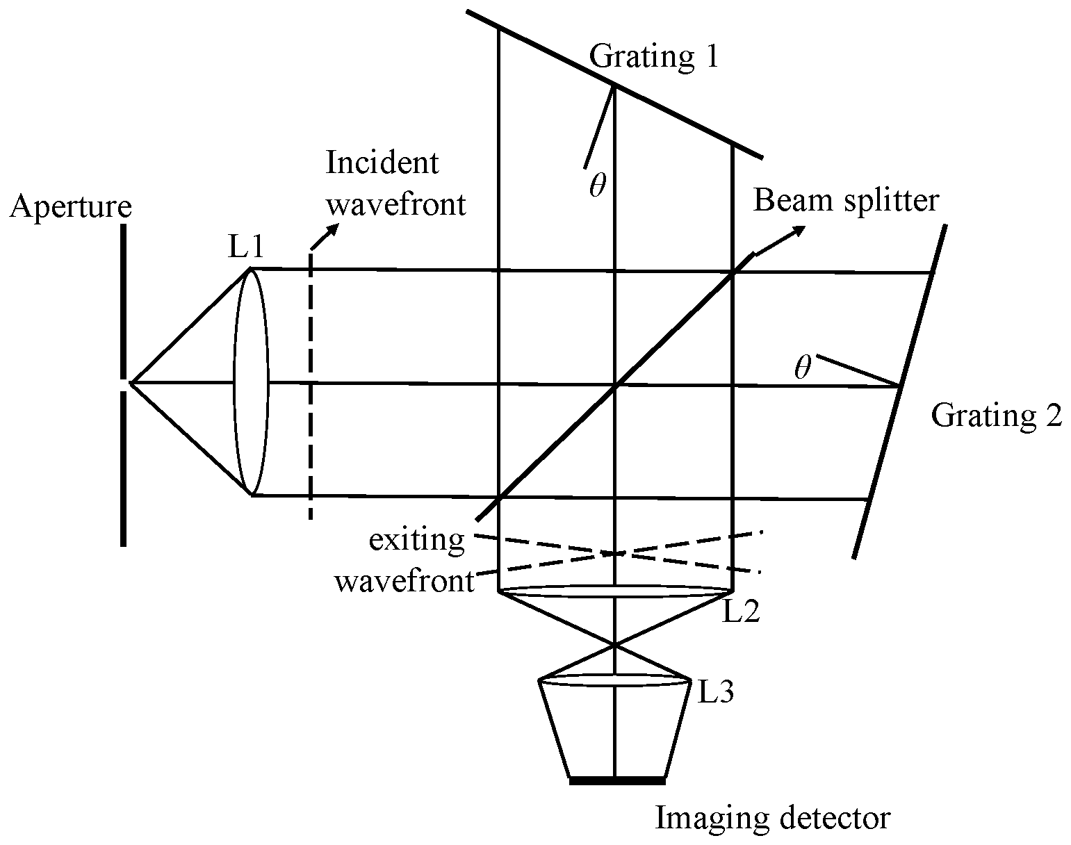
The DSHS is designed based on the principle of the spatial heterodyne spectrometer, of which the optical structure is shown in Fig. 1. The two planar mirrors in the traditional Michelson interferometer are replaced by two diffraction gratings (grating 1, grating 2). The light enters through aperture A and is collimated by the lens L1. It is split into two beams of coherent light of equal intensity by the beam splitter. One of them is reflected by the beam splitter and is incident on grating 1. The light is diffracted by grating 1 and returns to the beam splitter. The other light is incident on grating 2 through the beam splitter as well. It is diffracted by grating 2 and is reflected back to the beam splitter. The gratings are fixed and are placed at a Littrow angle θ with the orthogonal plane of the optical axis in the spatial-heterodyne-spectrometer system. The light is incident on the gratings by θ and is diffracted back with θ at some wavenumbers. It is called the light of the Littrow wavenumber σ0. The two exiting wavefronts of light of σ0 are diffracted by the gratings and are perpendicular to the optical axis. The phase difference is zero, and the interference fringe spatial frequency is zero, which cannot form the interferogram. However, the light of the non-Littrow wavenumber has a ±γ angle with the optical axis. The light forms the interferogram which will be imaged on the imaging detector by the optical imaging systems L2 and L3. So the two overlapping wave surfaces have an angle of 2γ which is calculated by Eq. (1) (Dohi and Suzuki, 1971):
where σ is the wavenumber of light, m is the order of diffraction, and 1∕d is the grating groove density. The angle between the light of the arbitrary wavenumber and the exiting light of the Littrow wavenumber is γ. The spatial frequency of the two σ light values is given by Eq. (2):
For the input spectrum B(σ), the intensity on the imaging detector is given by Eq. (3):
The spectral curve B(σ) can be recovered from the interferogram I(x) by a Fourier transform algorithm.
Furthermore, the spatial heterodyne spectroscopy can acquire a spatial distribution of one-dimensional spectral information through the two-dimensional detection technology. The scene in the field of view is divided into multiple field-of-view slices which are less than or equal to the number of rows in the focal-plane array by adding a cylindrical mirror to the front or rear optical system. The interferograms of each field-of-view slice are imaged on the corresponding detector rows respectively. The several rows on the detector correspond to layered spectral information in a field of view. The corresponding spatial-resolution unit on the detector can indicate the spatial information when the target signal appears in a certain range of lines. This means that the spatial heterodyne spectroscopy can obtain the radiance of atmospheric information at different altitudes simultaneously without scanning the atmosphere from one height to another height. It is important for monitoring the OH to reduce the time of data acquisition because the OH varies fast in the spatial and temporal dimension.

Figure 2Illustration of the double spatial heterodyne spectrometers. Panel (a) shows the vertical view of the DSHS, and panel (b) shows the overall mold of the DSHS.
2.2 Instrument innovation
The spatial heterodyne spectroscopy technology, an ultra-high-resolution spectroscopy technology used in the DSHS, has the characteristics of high flux, no mobile part, and a small size. The DSHS which is shown in Fig. 2 mainly consists of two spatial heterodyne spectrometers in the orthogonal layout to obtain enough data for inverting the OH concentrations. It includes the telescope cylinder system, the collimating system, the information-processing system, the imaging system, and some other optical components. The field-of-view angle is designed as 2∘. The spatial heterodyne spectrometer which scans along the satellite working orbit is defined as SHS1; the other which scans across the satellite working orbit is defined as SHS2. The scanning direction of SHS2 is orthogonal to that of SHS1 due to the special design of the orthogonal layout. The hierarchical detection of a series of observed radiance in the same target area becomes possible when the satellite flies along its orbital path. It means the sensor can obtain the data of each target height like in the multiangle method.
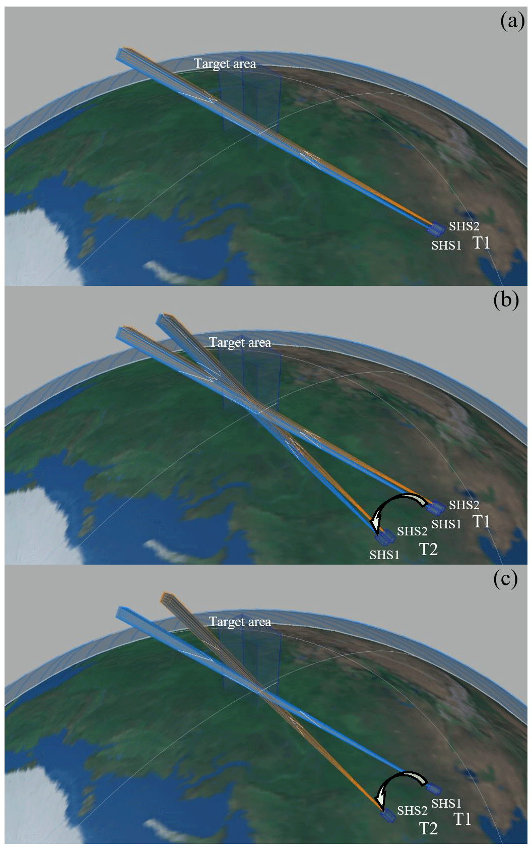
Figure 3Three-dimensional limb mode of DSHS at the time of T1 and T2 (a). The DSHS consists of two spatial heterodyne spectrometers (SHS1 and SHS2). The data of the target area cannot be obtained by the DSHS at the time of T1 and T2 (b). The DSHS monitors the OH in the target area using the data of SHS1 at the time of T1 and those of SHS2 at the time of T2 together (c). The arrows indicate the direction of the flight of the spacecraft.
The DSHS will detect the altitudes from 15 to 85 km by the three-dimensional limb mode. It can obtain the observed data in the target area along the satellite working orbit and across the satellite working orbit at the same time because SHS1 and SHS2 are orthogonal to each other. Figure 3 shows how the tomographic data are obtained by the three-dimensional limb mode.
As Fig. 3a shows, there are no intersection regions between the field-of-view slices of SHS1 and SHS2 at the time of T1. The tomographic data cannot be obtained in this situation. The three-dimensional structure of OH data is unable to be reconstructed. The data of SHS1 and SHS2 at different times will be used to obtain an intersection region for solving this issue. The different times which meet the requirements of the three-dimensional limb mode of the DSHS (we define one time as the time of T1 and the other time as the time of T2) are shown in Fig. 3b. At the time of T1, SHS1 and SHS2 finish a limb scanning in the vertical dimension (along the satellite working orbit) and the horizontal dimension (across the satellite working orbit). Then the satellite platform will need to reorient for obtaining the appropriate vector for the measurement at the time of T2 and will finish the observation project. The spectrometers are on during this process. The DSHS has the function of hierarchical imaging in the spatial dimensional which means it can obtain the data without scanning the target area. So the DSHS records at T1 and T2 are very brief. The line of sight at the time of T1 will intersect with the line of sight at the time of T2. The intersection region (target area) will form. However, the composition of tomographic data does not need all data from SHS1 and SHS2 at the time of T1 and T2. Some data should be omitted. As Fig. 3c shows, the field-of-view slices of T2-SHS2 (a horizontal-dimension spectrometer at the time of T2) are orthogonal to the field-of-view slices of T1-SHS1 (a vertical-dimension spectrometer at the time of T1) in an intersection region. The data obtained by SHS2 at the time of T1 and SHS1 at the time of T2 will be omitted in this measurement process. However, these data may be used for different measurements in other target areas to obtain the tomographic data when they meet the requirements of the three-dimensional limb mode. Thus, the three-dimensional segmentation of the target area will be complete. The three-dimensional division of the target atmosphere which consists of the intersection regions of SHS1 and SHS2 at different times is finally accomplished with the satellite platform moving. Different combinations of data for different intersection regions from two spatial heterodyne spectrometers are used to invert OH concentrations at different times.
The scanning direction will not be completely vertical or parallel to the surface when the DSHS is on the orbit but will have an angle η. So the satellite positions at the time of T2 where T2-SHS2 is orthogonal to T1-SHS1 in the intersection region are different with the η changing. In order to display and describe the satellite position of T2 conveniently, η is set to 0∘ temporarily. However, a unified set of η values is 30∘ in the relevant calculation during the pre-research phase.
The satellite positions and observation geometries are given at the time of T1. The satellite positions at the time of T2 need to be calculated for realizing the three-dimensional segmentation of the target atmosphere. This indicates that there are two satellite positions where the scanning directions of T2-SHS2 and T1-SHS1 are orthogonal to each other in the intersection region at the time of T2 based on the theory mentioned above. Figure 4 shows that there is a tangent point which is defined as P1 when the DSHS detects the atmosphere by the three-dimensional limb mode. The intersection region along the lines of sight of SHS1 (the blue line in Fig. 4) and SHS2 contains the observed data at the time of T1. There will be two lines of sight (the red lines in Fig. 4) where the scanning direction of SHS2 is orthogonal to that of SHS1s under the premise that the working altitude of the satellite is constant. The satellite position on the same side as the satellite position at the time of T1 is defined as the position at the time of T2-1, and the satellite position on the opposite side to the satellite position at the time of T1 is defined as the position at the time of T2-2. The two lines of sight at the time of T2 (T2-1 and T2-2) and a single line of sight at the time of T1 form two intersection regions R1 and R2 which are symmetrical about P1 along the line of sight at the time of T1. Figure 5 shows the relationship of the satellite positions at the time of T1 and T2 in space. These two intersection regions are on the two sides of the tangent point and are at the altitude of 500 km. The distance of the satellite position at the time of T2-2 from the position at the time of T1 is farther than the satellite position at the time of T2-1, which means the satellite needs more time to work from the position at the time of T1 to the position at the time of T2-2. The observed data will change a lot in this process and make a bigger difference in the target area at the time of T1. The satellite position at the time of T2-2 should be omitted. Meanwhile, the satellite position at the time of T2-1 is near the position at the time of T1; the observed data at the position of the time of T2-1 can reflect the OH distribution in the target area better because the OH information does not change too much in the short working time of the satellite. The distances between the intersection region and the tangent point determine the spatial resolution of the three-dimensional limb mode. That means the smaller the distance between the P1 and R1 (or R2) is, the higher the spatial resolution will be.
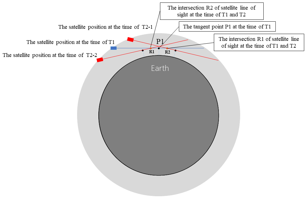
Figure 4Limb geometry diagram for the three-dimensional limb mode at the time of T1 and T2. The blue line is the line of sight of SHS1. The red lines are the lines of sight of SHS2.
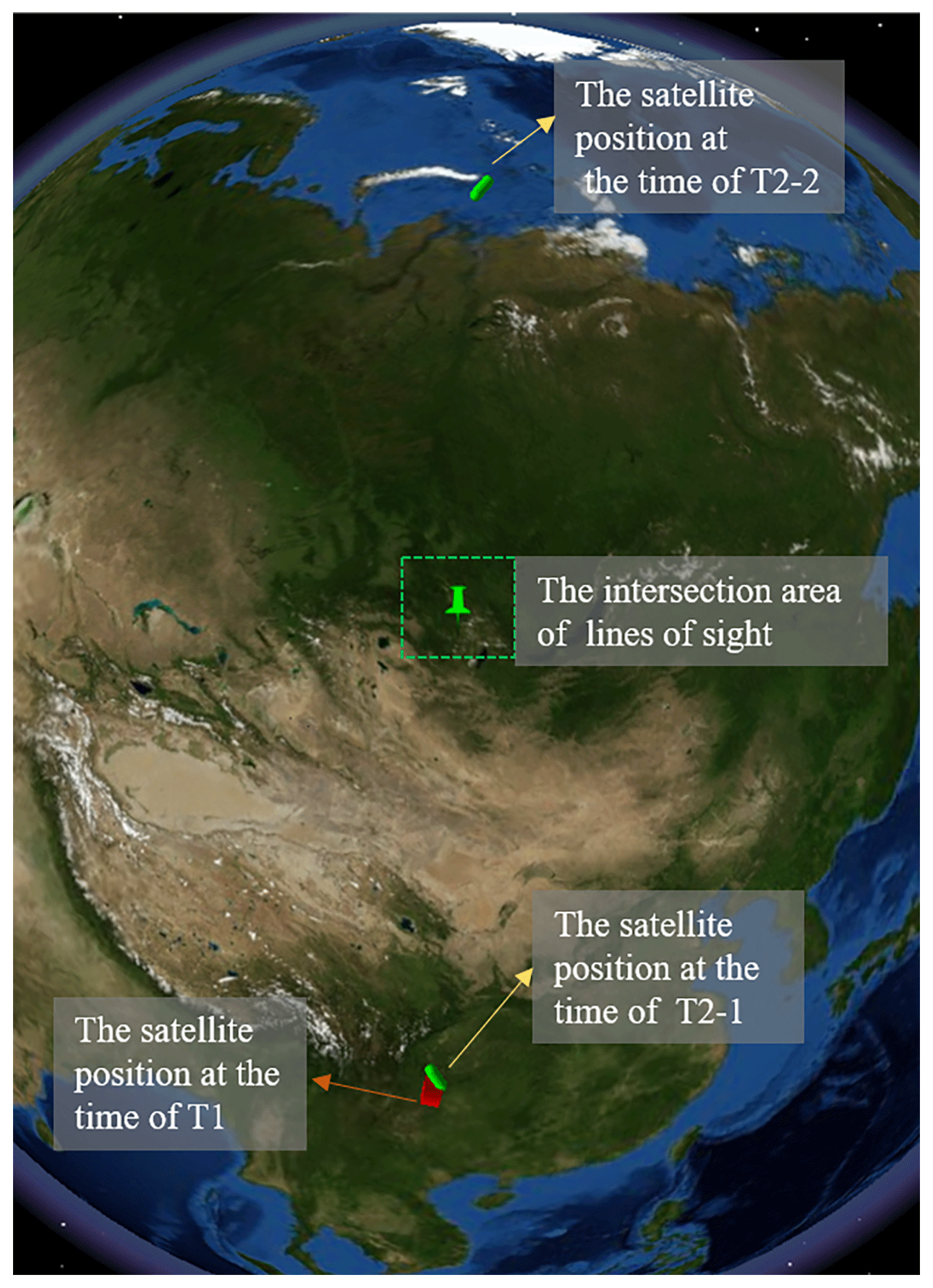
Figure 5Please check new figure.Relative location of the DSHS by the three-dimensional limb mode. There are two locations of the satellite at the time of T2 which meet the requirement of the three-dimensional limb mode. Map data: © Google Earth, Image IBCAO, and Landsat/Copernicus.
So the position at the time of T2-1 is picked up as the other satellite location where the field-of-view slices are orthogonal to each other at the intersection region. The OH concentrations at different heights are obtained by the combinations of observed data from SHS1 at the time of T1 and SHS2 at the time of T2 in the intersection region. Although the observed data are different because the geometric position and the viewing angle are different between the time of T1 and T2, the OH concentrations in the target area will be constant. The data are formed, and the structures of the observed data of SHS1 and SHS2 are the same in the three-dimensional limb mode. The distance between the intersection point R1 and tangent point P1 is presumed to be 50 km which is used in the subsequent research.
The forward model is used to express a physical process of how the atmospheric state parameter is obtained by the sensors. A precise forward model is significant for the design of the instrument and the retrieval algorithm. The observed data received by the DSHS with an ultra-high spectrum resolution are made up of two parts in this research: the atmospheric background radiance and the OH fluorescence emission radiance. The atmospheric background radiance is the result of the solar radiance being subjected to Rayleigh scattering and trace gas absorption. The OH fluorescence emission radiance is subjected to the OH fluorescence emission mechanism. These data can be simulated by a forward model which is constructed by the flowchart in Fig. 6.
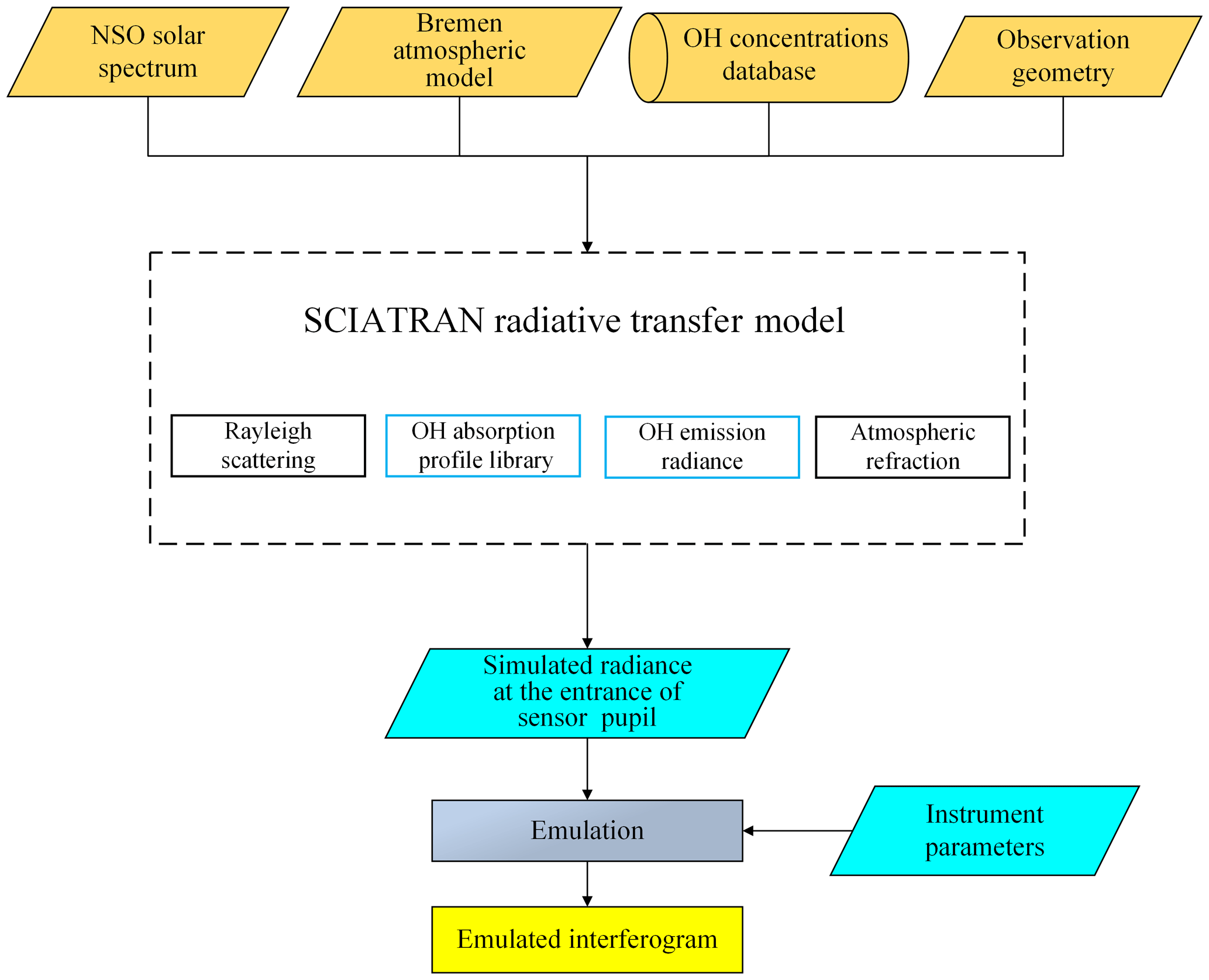
The forward model mainly constitutes by a radiative transfer model called SCIATRAN which has been developed for the Scanning Imaging Absorption Spectrometer for Atmospheric CHartographY (SCIAMACHY; Rozanov et al., 2014). However, some parts of it need to be modified for taking into account the characteristics of the DSHS and OH.
First, the radiance source, the solar radiation, is considered in this forward model for the radiance transmission of OH in the middle and upper atmosphere because (1) OH fluorescence emission radiance will be generated from the excited state to the ground state when the OH is excited by the solar radiation and (2) a high-precision calculation of the OH fluorescence emission radiance requires high-resolution solar radiation; the DSHS has a spectral resolution of 0.02 nm at least. The higher-spectral-resolution solar radiation will be used to obtain more realistic values. So the National Solar Observatory (NSO) solar spectrum with the resolution of nm is used for this forward model.
In addition to the NSO solar spectrum, the precision of the OH spectrum is also significant. SCIATRAN just takes the Rayleigh-scattered radiance function, the ozone absorption function, and the OH self-absorption function into account but ignores the effect of OH fluorescence emission radiance. LIFBASE software is used to calculate the OH emission spectrum in a temperature range according to the Bremen atmospheric model (Luque et al., 1999; Sinnhuber et al., 2009). The OH emission spectrum database is built up based on this. The database is put into SCIATRAN as a source function. The corresponding OH spectral emission data can be obtained from the database when the observed radiance is simulated at some conditions.
Next, the OH absorption spectrum database in SCIATRAN is based on the HITRAN 2012 database (Rothman et al., 2013) by default. However, the HITRAN 2012 database does not include the OH absorption profiles in the ultraviolet band. The OH absorption profiles in the HITRAN 2014 database are used to solve this problem. HITRAN 2012 is still retained, but the OH UV absorption line data from HITRAN 2014 are added into it.
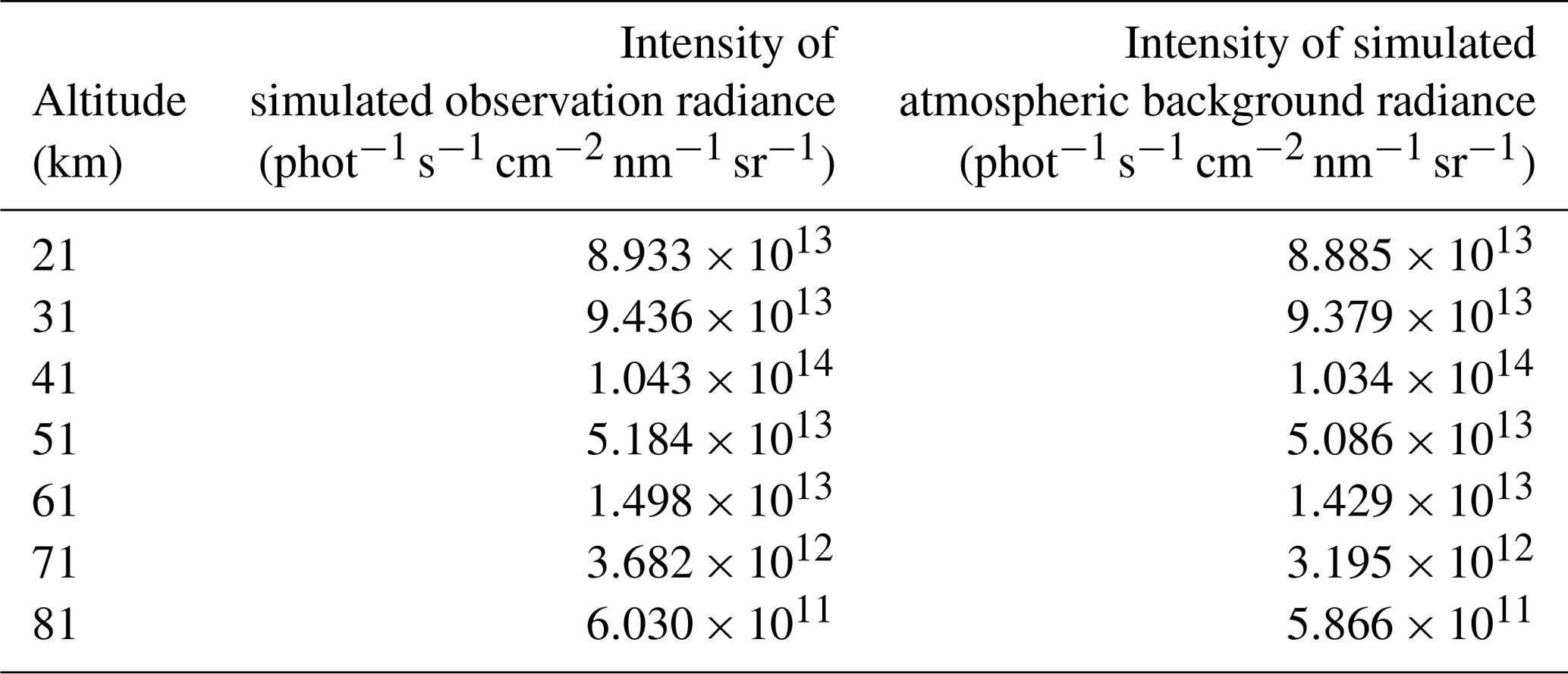
Finally, the precise atmospheric composition parameters are the assurance to simulate the observed radiance received by the sensors. That means the high-quality OH concentration database is needed when the radiance transfer is simulated accurately. For one thing, the MLS on the satellite Aura has monitored the global OH for many years, and the data can be acquired publicly at present. These data are used to build up the OH concentration database. The MLS was launched on 15 July 2004 aboard Aura and kept offering consequent OH data until 2009. It stopped monitoring from November 2009 to August 2011 to extend the service life of the sensor. It was restarted to monitor OH in August and September each year continually to obtain annual change trends in OH data. For another thing, the solar activity was relatively stable and maintained at a low level in the whole solar-activity cycle from 2005 to 2009. Solar activity from 2010 to 2016 was in an active cycle, and the level of solar activity in the next few years will be similar to the situation from 2005 to 2009. Therefore, the OH concentration data from 2005 to 2009 are a great reference for the research of atmospheric OH concentrations by the DSHS in the next few years. The MLS OH concentration Level 2 geophysical product is used to build up the OH concentration database and is averaged within a certain range for reducing the random errors. The N32 Gaussian grid from the European Centre for Medium-range Weather Forecasts is selected as the averaged method due to the random errors in MLS OH concentrations in high latitudes being much larger than those in low latitudes. It is a lattice-level coordinate system for the scientific model of spheres in Earth science. The latitude and longitude zones in the grid are divided unconventionally. The latitude band intervals of the Northern and Southern hemispheres are symmetrical about the Equator. The latitude band intervals and the number of longitude bands on a latitude gradually decrease with the increase in the latitude to ensure that each grid area is approximately equal. In addition, the four-seasons definition is used – the first quarter is March, April, May; the second quarter is June, July, August; the third quarter is September, October, November; the fourth quarter is December, January, February – as the temporal resolution for the OH concentration database. The season is the first quarter, and the OH concentration database is the N32 seasonal database. The simulated atmospheric background radiance is mainly subjected to the function of Rayleigh scattering, ozone absorption, and OH self-absorption. It is calculated based on some parameters such as the spatial, temporal, and observation geometries. An observed radiance profile is given as an example in the 27∘ N, 106∘ E area shown in Fig. 7. The intensity of simulated observation radiance and atmospheric background radiance at some tangent heights is also given in Table 1.

Table 1The intensity of simulated observation radiance and atmospheric background radiance at some tangent heights.
The results of the modified SCIATRAN will be imaged in the imaging system which collects complete data from all pixels on one line of the CCD. The digital number (DN) values of each pixel in each row are generated by Eq. (4) at different tangent heights:
where i is the number of rows along the line and j is the tangent height from 15 to 85 km. x(i) and y(j) are the areas where grating imaging images in the CCD; B(σ,y) is the input radiance spectrum; R(σ) is the instrument function; σ is the wavelength number, and θ is the Littrow angle. The interferogram will be obtained based on the instrument parameters in Table 2.
An emulated interferogram is shown in Fig. 8. It is the two-dimensional observed radiance interferogram constructed by 1024 columns which indicate numbers of interferogram samples and 36 rows which indicate the observed tangent heights. The observed radiance gradually increases to reach the peak value which is the brightness of the interferogram with the altitude increases until the altitude is around 40 km. The brightness decreases gradually until the upper limit of the detection height.
The errors in this forward model mainly depend on three factors based on the modified parts above: the atmospheric model, the Doppler effect, and the instrument calibration errors. First, the ozone in the atmospheric model is the influential factor that needs to be considered because its absorption cannot be ignored in the ultraviolet band. Second, the satellite has different heliocentric speeds when it flies over the area where the local solar time is noon or is around the morning faint line. The speed will lead to the shift in observed radiance at the ranges of the wavelength. Third, there are many sources of errors in the process of converting electrical signals into radiance values. The instrument calibration errors are assumed as ±5 % because the DSHS has not been officially in operation. The total errors in observed radiance are also given in Table 3. Zhang et al. (2017) have made a detailed analysis of errors and the reasons for them.
The DSHS is constituted by double spatial heterodyne spectrometers in the orthogonal layout. The distance between the intersection point and the tangent point is defined as 50 km, and the angle between the spatial-heterodyne-spectrometer scanning direction and the vertical and horizontal directions is defined as 30∘. The SHS2 positions at the time of T2 can be calculated according to the SHS1 observation geometry parameters at the time of T1 in the target area based on the detection theory of the three-dimensional limb mode. The simulated observation radiance of SHS2 and SHS1 can be obtained by the modified SCIATRAN described above. Some associated geometric parameters at the time of T1 and the calculated geometric parameters at the time of T2 are given in Table 4.
The intersection region at the time of T1 and T2 mentioned above is 67.46∘ N, 86.618∘ E. The observed radiance received by SHS1 at the time of T1 and received by SHS2 at the time of T2 is composed of a group of different satellite positions at tangent heights which is shown in Fig. 9.
Although the observation geometries and satellite positions are different at different times, both spatial heterodyne spectrometers scan the atmosphere by the same limb mode. The observed radiance profile still maintains the distribution in the band range from 308 to 310 nm. There are four global observed radiance databases for this research. The first-quarter observed radiance is given as an example; the NSO solar spectrum is used as the radiance source, and the Bremen global atmospheric model, the first-quarter OH concentration data of the N32 seasonal OH concentration database, and the geometric parameters of MLS OH production are also used to simulate the observed radiance in the band range from 308 to 310 nm at the time of T1 and T2. The results are shown in Fig. 10, which shows the observed radiance received by SHS1 at the time of T1, and Fig. 11, which shows the observed radiance received by SHS2 at the time of T2.
There are some differences between Fig. 10 and Fig. 11 because of the observed geometries and satellite positions. However, the overall observed radiance trends are the same. The observed radiance increases from 8×10¹³ to 1.4×10¹⁴ until the altitude at around 45 km and decreases to about 4×10¹³ with the altitude increasing. The lowest observed radiance is in the region around 30∘ N and gradually increases towards the two poles at about 41 km. The reason for this trend is that the solar zenith angle is the minimum value around 30∘ N and then increases towards the two poles. At 71 km, the observed geometries are not the only influencing factor and the distributions of OH concentrations are also influential. The Rayleigh-scattered radiance is weak, and OH fluorescence emission radiance becomes strong. In addition to this, the OH concentrations in the first quarter are low in the region around 60∘ N which makes the high radiance values appear in the Southern Hemisphere.

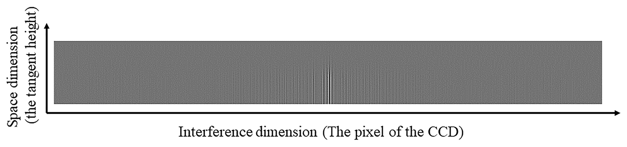
Table 3Total errors in observed radiance caused by different factors at some tangent heights.
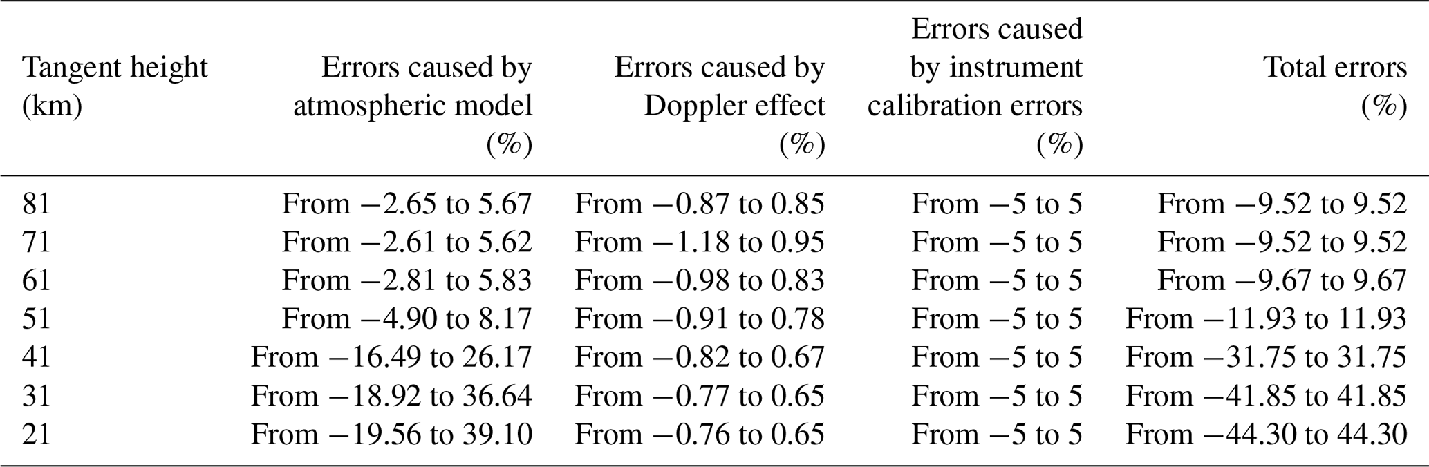
Table 4Locations and geometry parameters of SHS1 at the time of T1 at some tangent heights and the corresponding parameters of SHS2 at the time of T2.

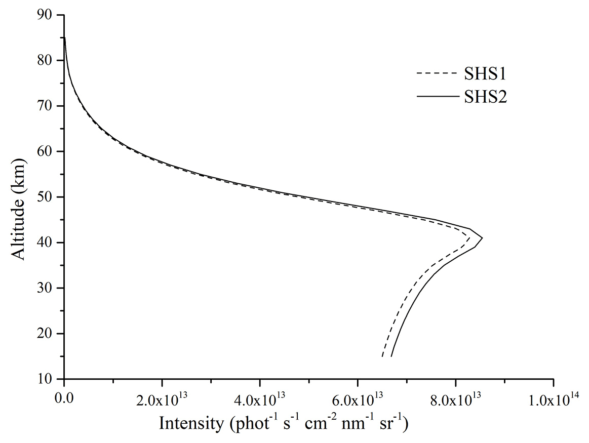
Figure 9The simulated observation data in the intersection region at the time of T1 and T2. The dashed line is the simulated observation data received by SHS1 at the time of T1, and the solid line is the simulated observation data received by SHS2 at the time of T2.
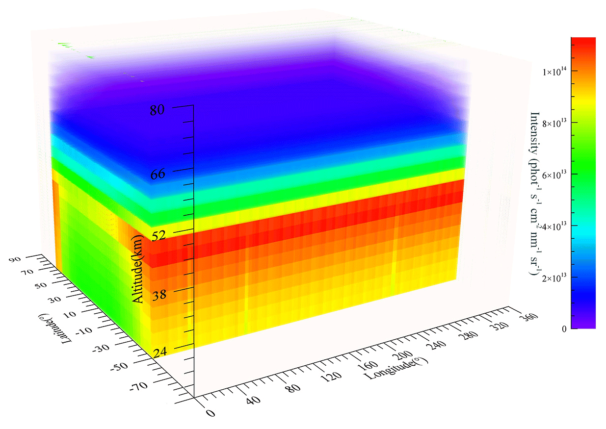
Figure 10The simulated observation radiance received by SHS1 at the time of T1 under the different conditions.

Figure 11The simulated observation radiance received by SHS2 at the time of T2 under the different conditions.
4.1 Interferogram pretreatments
The method of forming the interferogram by spatial heterodyne spectroscopy is spatial heterodyne modulation. The signal-to-noise ratio is susceptible to many factors, and the fine spectral lines of the noisy signal can also be detected simultaneously. The interferogram needs to be pretreated for solving these problems and transformed to obtain the OH fluorescence emission radiance. All the pretreatments are shown in Fig. 12.
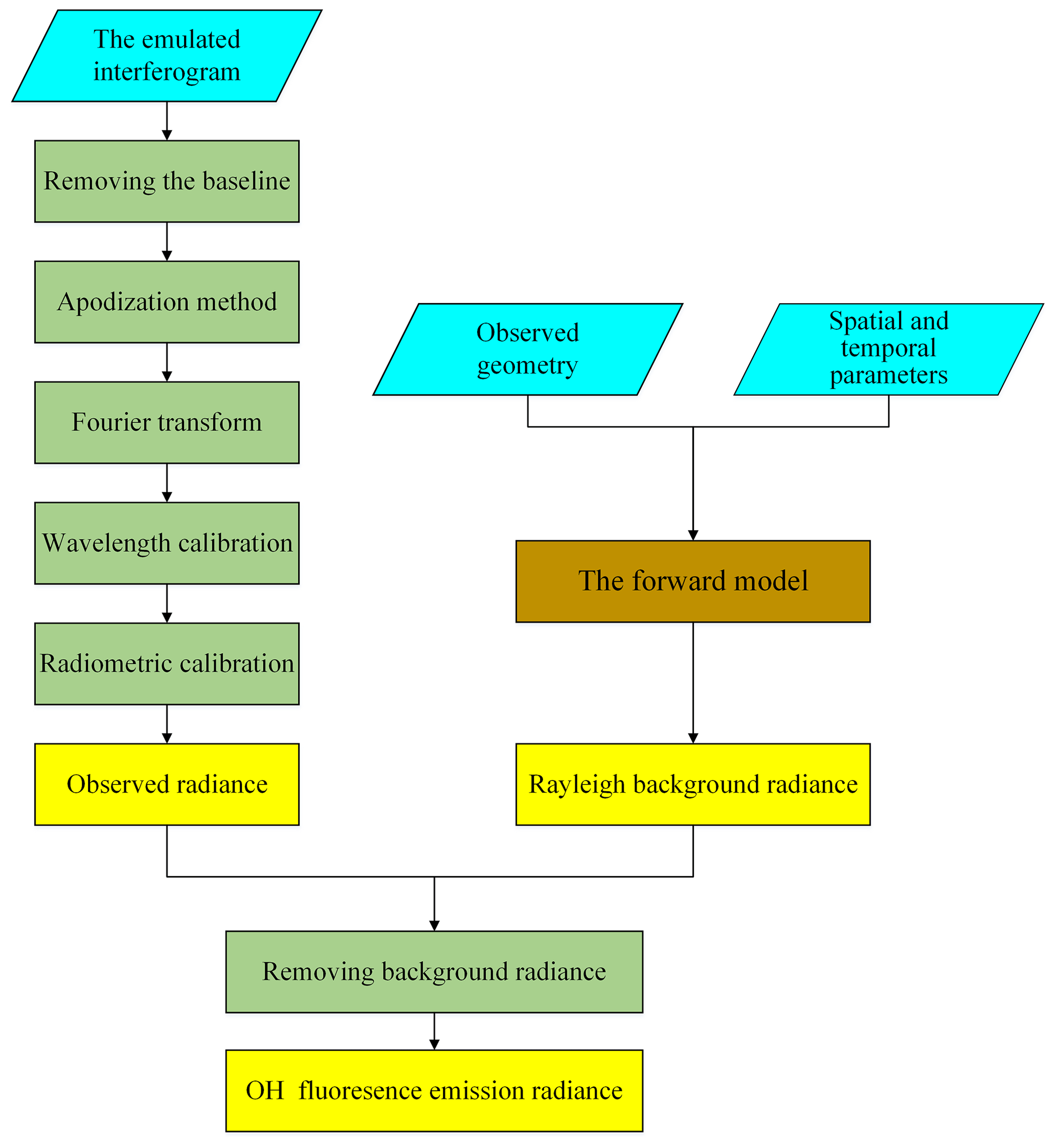
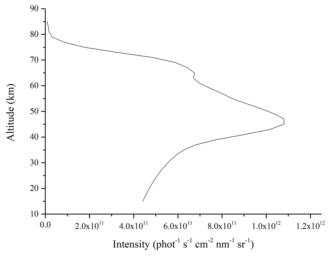
First, the interference data with a low-frequency baseline will make low-frequency spurious signals in the process of the Fourier spectrum transform. The methods of removing the baseline mainly include the polynomial linear fitting to the baseline and the first-order differential de-baseline method at present. The function of the first-order differential de-baseline method is high-pass filtering. It is the most useful way to remove the baseline (Ye et al., 2009). The interferogram obtained by the spatial heterodyne spectrometer is the interference data in the interval of the finite optical-path difference from −L to +L. That means an interferometric function forces a sudden drop to zero outside of this range. It will cause the interferogram to appear with sharp discontinuities in the edge interval. The spectral profile has side lobes in which the positive side lobes are the source of the false signal and the negative side lobes will lead to the adjacent weak spectral signals being submerged. The apodization method is used to mitigate the discontinuity of the interferogram edge through multiplying the interferogram function by a progressive weight function. The interferogram after apodization is subjected to the Fourier spectrum transform for obtaining the corresponding spectrum. However, the high-spectral-resolution observed radiance data which are simulated by the forward model mentioned above include the atmospheric background radiance. It must be identified and removed from the observed radiance data before the OH fluorescence emission radiance is obtained because (1) the atmospheric background radiance accounts for more than 95 % of observed radiance that will make OH fluorescence emission radiance low and (2) some errors in atmospheric background radiance will transfer into the OH fluorescence emission radiance when the observed radiance of the interferogram form is recovered in the spectral form. The intensities of simulated observation radiance and atmospheric background radiance at some tangent heights are given in Table 1. The OH fluorescence emission radiance can be calculated by subtracting the atmospheric background radiance from the observed radiance. The OH fluorescence emission radiance graph which is shown in Fig. 13 can be obtained after these steps, and the Fourier spectrum transform can be performed.

The fifth step is the wavelength calibration. The zero position of the spectral data points corresponds to the Littrow wavelength number in the Fourier transform spectrum, so the wavelength calibration equation is given by Eq. (5):
where i is from 0 to 1024. δi is the symbol of intensity (). The sixth step is the radiometric calibration. The purpose of the radiometric3 calibration is to determine the quantitative relationship between the output signal of the instrument and the spectral radiance because the spectrometer obtains the DN values directly. A linear-fit method is used to simulate the different sets of known radiance values at each spectral data point for establishing a fitting relationship in the calibration process by Eq. (6):
where Sδ is the DN value at the wavelength number δ. Bδ is the assumed incident spectrum radiance. Kδ is the calibration factor, and εδ is the deviation caused by other factors. A spectrum of OH fluorescence emission radiance is shown in Fig. 14.
4.2 Constructions of the retrieval algorithm
It is an inversion process to obtain the OH concentrations by the DSHS observed radiance. The observed radiance is simulated through the forward model in this research. However, OH concentrations cannot be obtained in an inverse way directly. The atmospheric-inversion problems are not an inversion of the forward model but use some related algorithms to estimate the atmospheric parameters for finding the best state parameters through the observed radiance data. The DSHS consists of two spatial heterodyne spectrometers in the orthogonal layout for monitoring the OH from 15 to 85 km. It will provide many complicated data. The traditional iterative retrieval algorithm will take more time to obtain the OH concentrations in this case because of the character of iteration. A new retrieval algorithm that is suitable for the DSHS needs to be constructed for inverting the accurate OH concentrations.
The precondition of the three-dimensional limb mode for monitoring the OH is that the time interval must be relatively short. Otherwise, the OH concentrations will change. The observed data cannot reflect the accurate OH concentrations. The distance between the satellite positions at the time of T1 and T2 is approximately 66 km when the intersection point is assumed to be 50 km away from the tangent point mentioned in Sect. 2. So the intervals between those points are very small. Additionally, the OH concentrations do not change much in a very short time according to MLS products. The short interval time between T1 and T2 and small changes in OH concentrations in a very short time support the theoretical premise of the new retrieval algorithm and make it possible for the DSHS to detect the atmosphere by the three-dimensional limb mode. An algorithm called the tomographic retrieval algorithm is constructed to invert OH concentrations from 15 to 85 km based on the theory described above. The core of this retrieval algorithm is the lookup table method. The most important step for it is the construction of the tomographic-observation database. The main influence factors for making up the tomographic-observation database comprise the atmospheric model, the observation geometries (the solar zenith angle and the relative azimuth angle), the spatial information (position of the target area and satellite position), date parameters, the OH concentrations, and the simulated observation data. The solar zenith angle and the relative azimuth angle have a greater influence on the observed radiance. The spatial information and date parameters will affect the OH concentrations and the atmospheric model. The solar zenith angle is changed between 0 and 100∘, and the relative azimuth angle is changed between 0 and 180∘. The corresponding OH concentrations are found according to the date parameters and spatial information such as the season, latitude, and longitude of the target area from the OH concentration database which has been built up as described in Sect. 3. The OH concentrations are changed in the range of between 50 % and 150 % of the amount of the original corresponding concentration at different tangent heights for more probable situations. Many combinations of various state parameters can be generated according to these changes. The observed data received by DSHS in these combinations are simulated through the forward model mentioned above. The tomographic-observation database can be built up for the tomographic retrieval algorithm. Each parameter that is part of the database is accurate, and the errors in the parameters are analyzed in Table 3. The method of constructing the database is reasonable, which is shown in Fig. 15. Table 5 gives an example of a subset of rows of a part of the tomographic-observation database. SZA is the solar zenith angle; AA is the relative azimuth angle; MultiND_height is the tangent height.
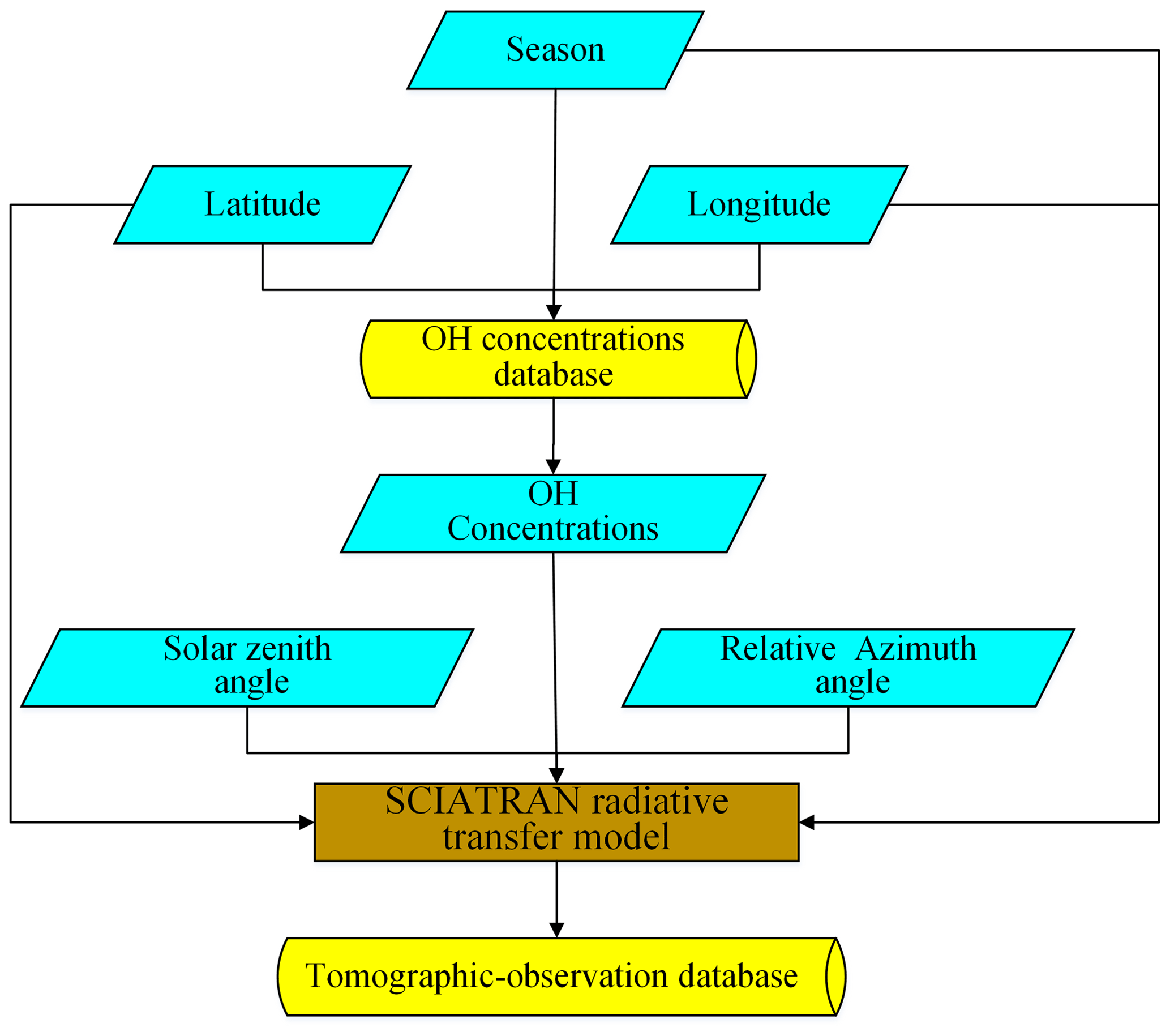
Table 5A subset of rows of the tomographic-observation database.

Based on the satellite positions, the observation geometries, the date parameters, the observed radiance at all wavelengths of SHS1 at the time of T1, and the corresponding observed radiance at all wavelengths of SHS2 at the time of T2, the OH concentrations in the target area can be found in the tomographic-observation database directly. The tomographic-observation database is effective and reasonable enough. However, it is impossible to include all combinations in the tomographic-observation database because (1) the size of the tomographic-observation database is limited and (2) all situations of when the sensor will be working in the orbit cannot be considered. Interpolation methods and threshold judgment methods are always used to solve such problems. A scientific and precise threshold in the threshold judgment method can be obtained according to a lot of OH concentration data and experiments. The OH concentration data are currently few. So if there is no corresponding query condition in the database, the cubic spline interpolation is used to calculate the OH concentrations. The cubic spline interpolation not only has higher stability than other interpolation algorithms but also can maintain the continuity and smoothness of the interpolation function under the premise of convergence. Figure 16 shows the flowchart of the tomographic retrieval algorithm that obtains the OH concentrations.
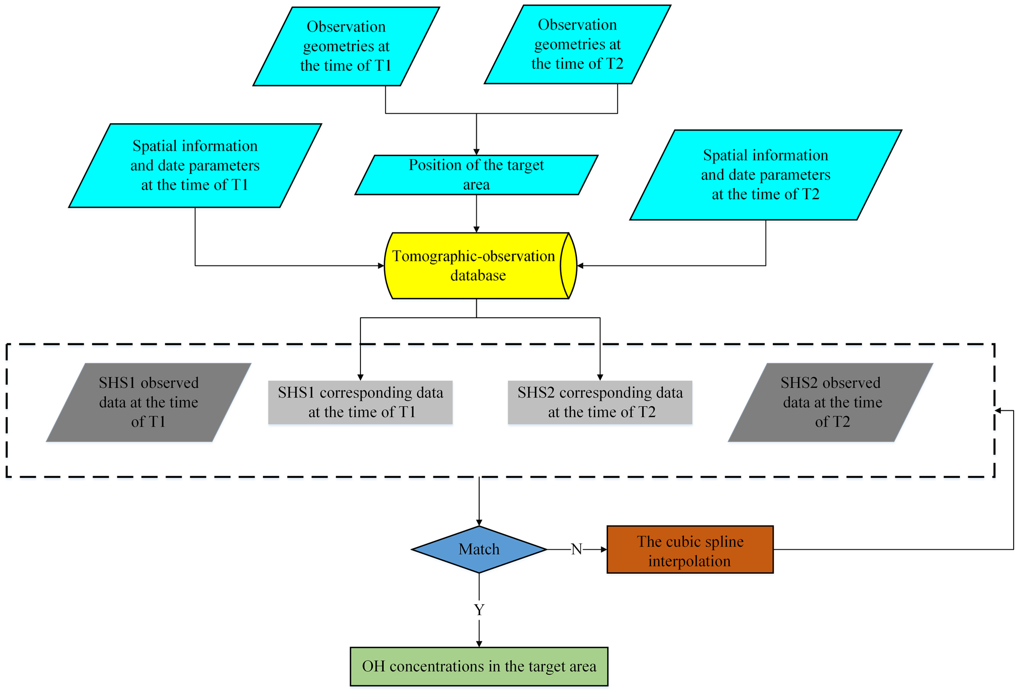
Figure 16Flowchart of the tomographic retrieval algorithm. The OH concentrations can be obtained from the tomographic-observation database or by the cubic spline interpolation.
5.1 Inversion results
There are four tomographic-observation databases based on the four seasons. The profile data in the database are averaged to obtain the monthly average concentration profile data. So it will not introduce discontinuities to the retrieved OH time series when an abrupt switch happens. Here, the spring season tomographic-observation database is used as an example to prove the feasibility and superiority of the tomographic retrieval algorithm. The OH concentrations are obtained in the (67.46∘ N, 86.168∘ E) through satellite positions, observation geometries, date parameters which are given in Table 5. If there is a corresponding query condition, the OH concentrations can be given directly from the tomographic-observation database. Otherwise, the OH concentrations will be calculated by the cubic spline interpolation. The inversion results are shown in Fig. 17.
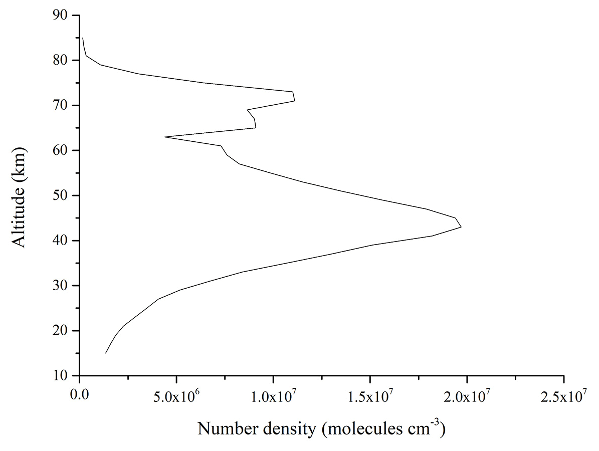
The results indicate that a maximum peak value of OH concentrations is about 2.0×10⁷ molecules cm−3. It appears at around 45 km which closely relates to the ozone concentrations in the stratopause as the heights increase. A valley value of OH concentrations about 5.0×10⁶ molecules cm−3 appears around 65 km. As the height continues to rise, the second maximum peak value of OH concentrations about 1.0×10⁷ molecules cm−3 appears at around 70 km which is mainly affected by the water vapor concentrations in the mesosphere. The OH concentrations above the 75 km and below the 25 km is very low (about 2.5×10⁶ molecules cm−3). In general, the OH concentrations increase with the altitudes rise until around 40 km and reach the valley value at around 65 km. The second maximum value peak which is affected by the water vapor concentrations appears at around 75 km, then the OH concentrations continue to decrease until the limited altitudes of detection.
5.2 Discussion
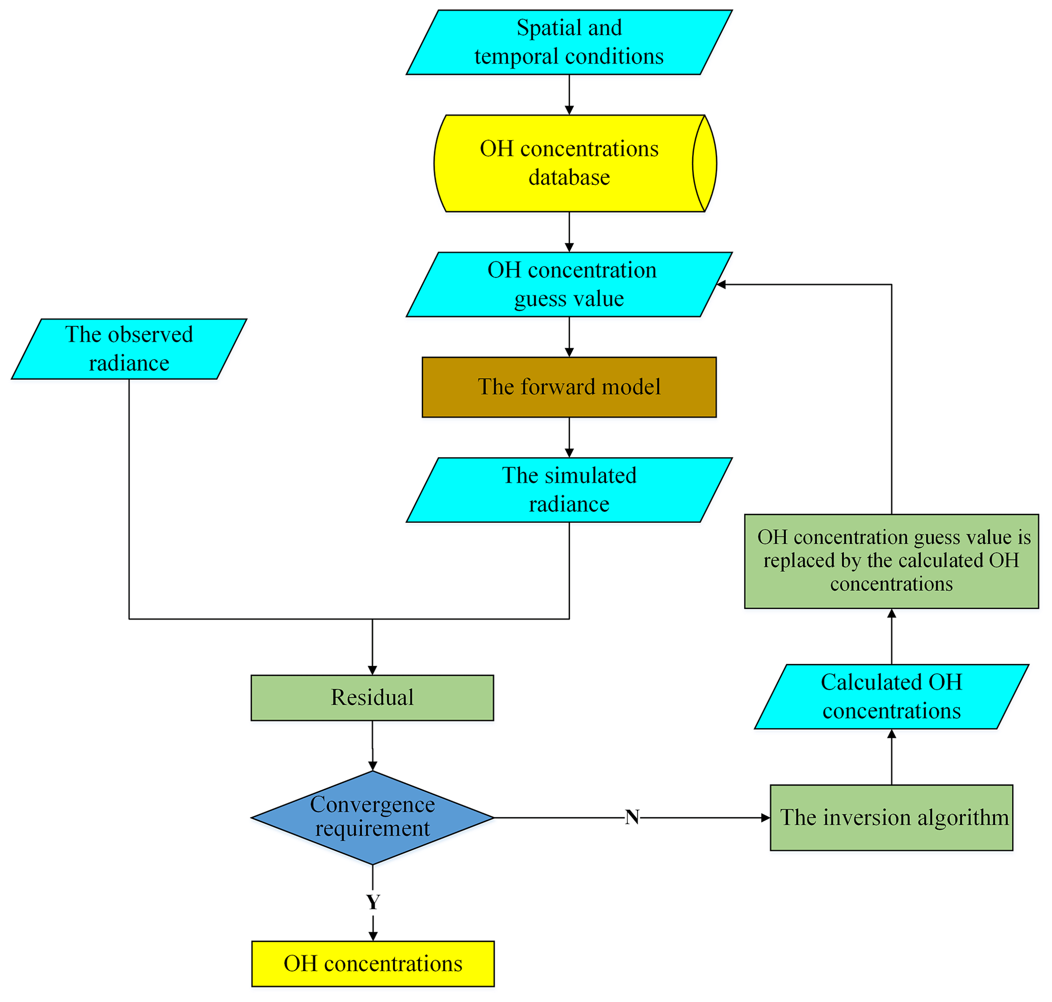
We also constructed an iterative retrieval algorithm to compare with the tomographic retrieval algorithm here for reflecting the outstanding advantages of the tomographic retrieval algorithm. The schematic diagram of iterative inversion is shown in Fig. 18. The simulated radiance can be obtained under the condition which an initial OH concentration guess can get from the OH concentration database. The residuals of the simulated and observed data will be calculated to judge the convergence. The initial OH concentration guess values are the inversion results if the residual meets the accurate requirements of the research. Otherwise, the retrieval algorithm will be used to obtain the inversion results.
The LSUV (Limb scan of Scattered UV radiation) retrieval algorithm (Aruga and Heath, 1988; Aruga and Igarashi, 1976) is modified to invert OH concentrations at each tangent height. The tangent height is defined as m and the target area is divided into n atmospheric layers from the bottom to the top. One-order approximate Taylor expansion is used to establish a linear relationship between the OH concentrations and observed radiance at each atmospheric layer by Eq. (7):
where εi, the inversion coefficient, is approximately 1 when the OH concentrations are close to the guess OH concentrations. Fi is the difference between the observed data and simulated data by Eq. (8) at the i layer:
Dij which is given by Eq. (9) is the partial derivative of radiance data at the i tangent height:
yj in Eq. (10) is the relative error between the OH concentrations N(j) which can be obtained through yj and Ng(j) when the convergences meet the accurate requirement or the number of iterations exceeds the threshold of the iteration number and the guess concentrations Ng(j):
The approximate OH concentrations at each tangent height (Q)i can be obtained based on Eq. (10) and Eq. (11):
The approximate OH concentrations (Q)i at the i tangent height are determined by the OH concentrations in several atmospheric layers near i. The weight function Pij is established from Dij by Eq. (12):
where Pij is the proportion of the contribution of OH concentrations to the radiance of each tangent height in each layer. The accurate relative errors in the OH concentrations and guess OH concentrations in each layer yj can be obtained from Pij by Eq. (13):
However, the difference between the OH concentrations and guess OH concentrations is large in the actual satellite detection; εi is not 1, and is used to replace it by Eq. (14):
Finally, the precise relative error yj between the OH concentrations and the guess OH concentrations can be obtained. The OH concentrations N(j) can be obtained through yj and Ng(j). The convergence error between the observed data I(hi) and simulated data Is(hi) at the i layer which is based on the guess OH concentrations Ng(j) is calculated by Eq. (15):
where l is the number of iterations. The average residual Rl based on at different tangent heights can be calculated by Eq. (16):
The threshold of the average residual and the numbers of iterations are set based on the inversion experience. The iteration result which meets the precision requirement is the final result; otherwise the prior Ng(j) will be replaced by the N(j) which is calculated by the inversion algorithm, and the iteration process will continue until the residual convergences meet the accurate requirement or the number of iterations exceeds the threshold of the iteration number. The iteration stops when the average residual decreases below 0.005 or the number of iterations reaches 15 in this research.
The observed radiance which is simulated by the forward model is used by the LSUV retrieval algorithm to invert OH concentrations. When the iteration results meet the accurate requirements of the research, the OH concentrations can be obtained. The OH concentrations obtained by the LSUV retrieval algorithm are credible in the upper atmosphere which are the same as the results of MAHRSI and SHIMMER (Conway et al., 1999; Englert et al., 2010). However, the OH concentrations in the lower atmosphere such as below 30 km are unsuitable for scientific research because the interference factors like water vapor and ozone are too large. A single spatial heterodyne spectrometer with a traditional limb mode also cannot obtain enough high-quality data to invert the OH concentrations, which would make the inversion results unscientific especially in the lower atmosphere. That is the reason why there are no OH concentrations in these regions from the MAHRSI and SHIMMER (Harlander et al., 2002).
The tomographic retrieval algorithm and the LSUV are two independent algorithms. The tomographic retrieval algorithm effectively avoids the constraints of the initial guess values and does not take a lot of time to iterate to obtain the results in the inversion process. The errors in this retrieval algorithm just include the errors caused by the interpolation method and the observed radiance errors which are used in the algorithm. The observed radiance errors are affected by the atmospheric model, the Doppler effect, and the instrument calibration errors. The OH fluorescence emission radiance which is separated from the observed radiance is the most important part for the OH concentrations, so the contributions of each part to the OH fluorescence emission radiance are analyzed by the following method. Some certain amounts calculated as the disturbances are applied to the three parts above. The OH fluorescence emission radiance obtained based on these parts is considered incorrect. The original parts are taken as the actual and undisturbed parameters; the results based on these parts constitute the true OH fluorescence emission radiance. The relative errors between the true and incorrect OH fluorescence emission radiance are calculated by Eq. (17):
where [I]err is the incorrect OH fluorescence emission radiance and [I]act is the true OH fluorescence emission radiance.
5.2.1 Influence of the atmospheric model
The atmosphere environment is complicated. Although, the atmospheric model used in this research is scientific and reasonable, it cannot reflect accurate atmospheric conditions which leads to some errors between true OH fluorescence emission radiance and incorrect OH fluorescence emission radiance. These will cause an error when the OH concentrations are looked up or calculated. Many factors can affect the OH fluorescence emission radiance in the atmospheric model such as some physical parameters like temperature and pressure and some atmospheric components like nitrogen dioxide and formaldehyde. Here, the main composition we consider is ozone which is a substance that plays a major role in the process of radiation transmission as solar energy in the ultraviolet band and is the main source and sink of OH radicals. The other relevant source of uncertainty will be considered in following research when the DSHS works on the orbit. The original ozone profiles are assumed to be the actual atmospheric state parameter, and the ozone profile for the disturbances is set as ±30 % (Conway et al., 2000). The relative errors in the OH fluorescence emission radiance caused by the atmospheric model are calculated by Eq. (17) and are shown in Fig. 19. The relative errors in the OH fluorescence emission radiance at some tangent heights are also given in Table 6.
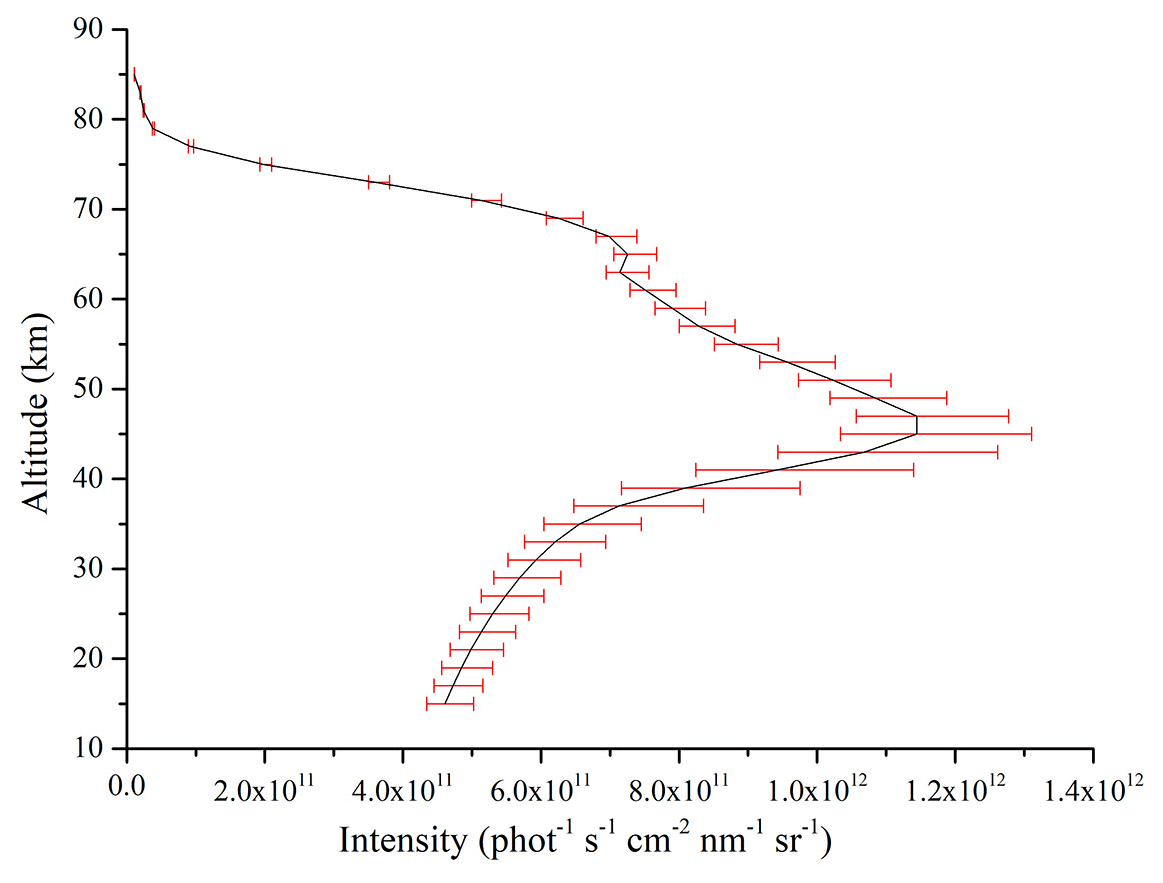
Figure 19Relative errors in OH fluorescence emission radiance caused by the atmospheric model in the tomographic retrieval algorithm. The red error bars indicate the relative errors caused by the atmospheric model.
Table 6Relative errors in OH fluorescence emission radiance caused by the atmospheric model at some tangent heights.
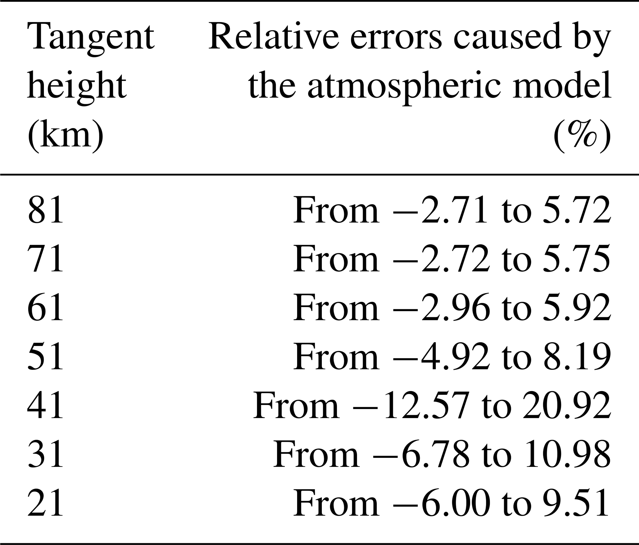
The relative errors caused by the atmospheric model indicate that the atmospheric model has a strong impact on the OH fluorescence emission radiance, especially in the lower atmosphere where the ozone concentrations are high. The errors caused by a ±30 % uncertainty in the atmospheric model have a peak value from −12.57 % to 20.92 % at the 41 km. It also appears by the same calculation method from −12.19 % to 20.28 % in the LSUV retrieval algorithm. The concentrations of ozone gradually decrease with the relative errors decreasing to about −3 % to 5 % when the heights increase. The effect of the atmospheric model is smaller in the upper atmosphere. The distribution of errors has the same tendency in the LSUV retrieval algorithm in that the relative errors increase and then gradually decrease after reaching the peak value of altitude. These mean the relative errors caused by the atmospheric model are inevitable. If the more current atmospheric model is used, more accurate OH fluorescence emission radiance may be obtained, which is the key for the retrieval algorithm.
5.2.2 Influence of the Doppler effect
The satellite has different heliocentric speeds on its working orbit around the Earth at different times. It will cause a pseudorandom offset of observed data within nm at the range of the wavelength. The observed radiance is calculated within nm of disturbance at the wavelength. The OH fluorescence emission radiance which is separated from the observed radiance is too weak.
A small Doppler effect will cause a great influence on the weak OH fluorescence emission radiance. The magnitude of wavelength shift caused by the Doppler effect is much smaller than the spectral resolution. The “finding-peak” method is used to find a peak value which needs to be larger than the values on its sides. It is impossible to correct the offset by the finding-peak method. However, the “taking-peak” method is defined to find the highest peak value in the OH fluorescence emission radiance. The taking-peak method is used for reducing the impact of the Doppler effect. Therefore, the OH fluorescence emission radiance at the peak position is used instead of the wavelength from 308 to 310 nm when calculating the relative errors caused by the Doppler effect at a single tangent height. The relative errors in the OH fluorescence emission radiance caused by the Doppler effect are calculated by Eq. (17) and are shown in Fig. 20. The relative errors in OH fluorescence emission radiance caused by the Doppler effect at some tangent heights are also given in Table 7.
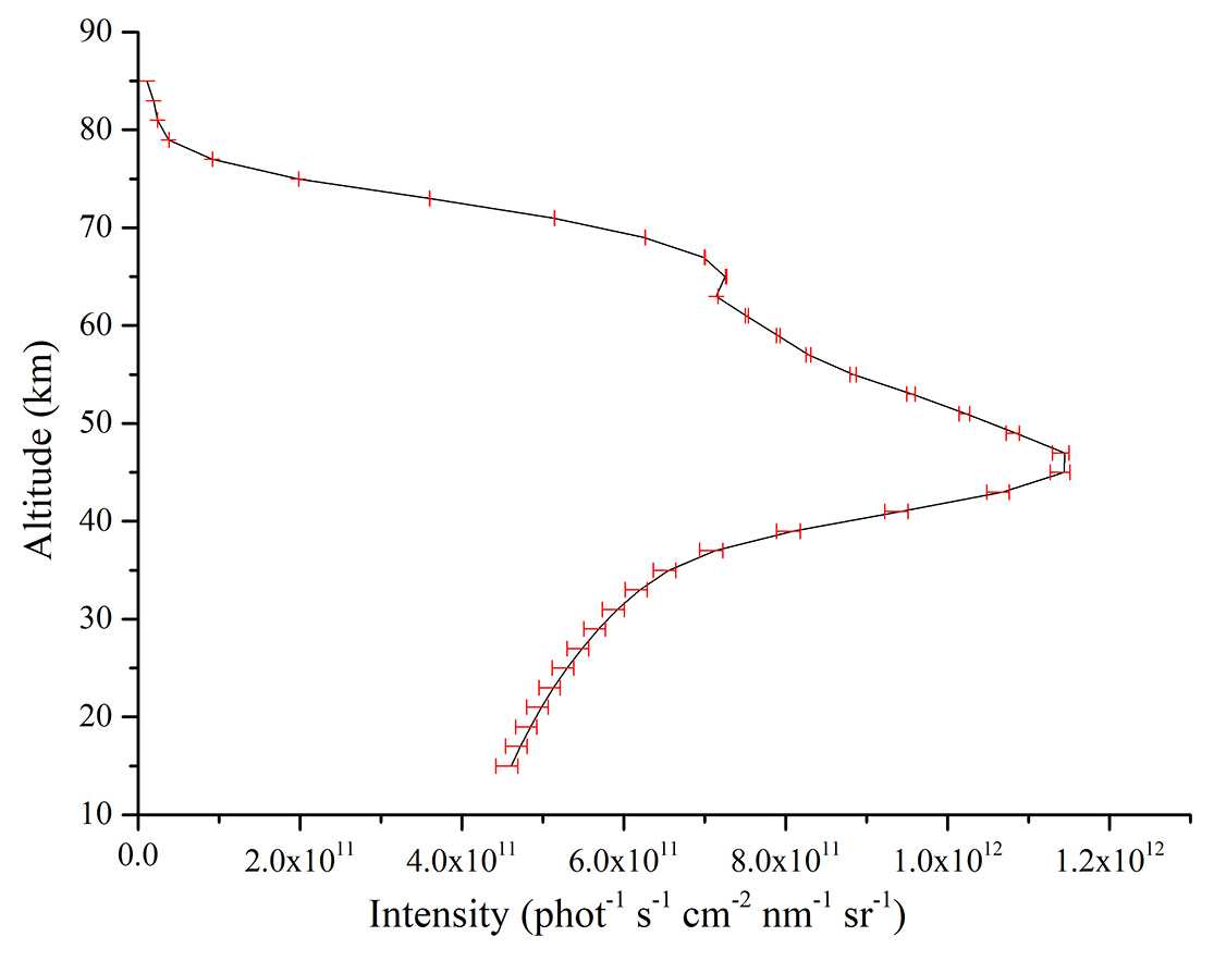
Figure 20Relative errors in OH fluorescence emission radiance caused by the Doppler effect in the tomographic retrieval algorithm. The red error bars indicate the relative errors caused by the Doppler effect.
Table 7Relative errors in the OH fluorescence emission radiance caused by the Doppler effect at some tangent heights.
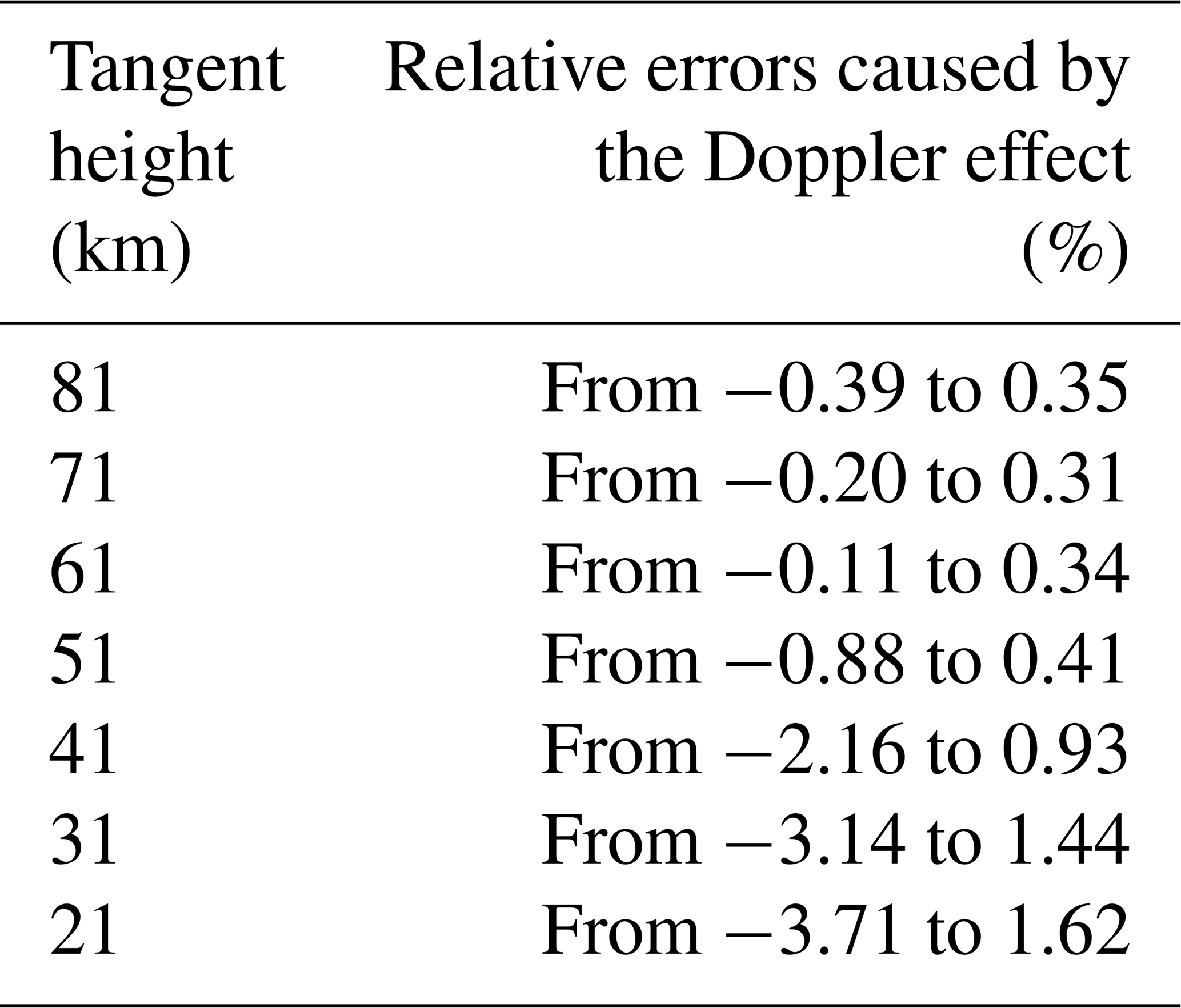
The relative errors in OH fluorescence emission radiance caused by the Doppler effect decrease when the altitudes rise. The tendency of relative errors is the same, but the relative errors in the tomographic retrieval algorithm are smaller than in the LSUV retrieval algorithm. This indicates that the tomographic retrieval algorithm can obtain more accurate OH concentrations than the LSUV retrieval algorithm although the errors caused by the Doppler effect cannot be avoided when the spectral resolution of the DSHS is extremely high.
5.2.3 Influence of other factors
Some other errors exist apart from the errors described above. For one thing, there are various sources that make some errors between the radiance received by the sensors and the actual radiance in the instrument calibration process. The instrument calibration errors will cause an error in the inversion result. We assumed the instrument calibration errors are ±5 % in this research after referring to the detector parameters that due to the DSHS do not officially work (Ye et al., 2009). For another, the error caused by the interpolation method is the main factor we need to calculate. The cubic spline interpolation not only has higher stability but also can ensure the continuity and smoothness of the interpolation function under the premise of ensuring the convergence compared with other interpolation methods like the linear-interpolation method. The error estimation of the interpolation results is as accurate as possible. The OH concentrations can be obtained by the tomographic retrieval algorithm according to the atmospheric model, spatial information, date parameters, observation geometries, and observed radiance. The interpolation errors are also the other error factors which affect the accuracy of OH concentrations. We give a certain disturbance value to different parameters for calculating the effect of the interpolation algorithm on the OH concentrations. The solar zenith angle is changed between 0 and 100∘, and the magnitude of perturbation is 10∘. The relative azimuth angle is changed between 0 to 180∘ and the magnitude of perturbation is also 10∘. The OH concentrations are changed in the range between 50 % to 150 % of the amount of the original corresponding one at different tangent heights for more probable situations, and the magnitude of perturbation is 10 %. The date parameters, longitude, and latitude can determine the atmospheric model. So the influence of date parameters, longitude, and latitude is calculated through disturbance of the ozone concentrations, and the magnitude of perturbation is 30 % of the amount of the original corresponding one. It is about 0.32 % for the six-dimensional cubic spline interpolation of the OH concentrations, date parameters, longitude, latitude, solar zenith angle, and azimuth angle after research and related experiment. Therefore, 0.32 % is taken as the error in the interpolation algorithm in the tomographic retrieval algorithm.
5.2.4 Analysis of total errors in the OH concentrations
The errors in retrieved results must be considered after the discussions about the errors in OH radiance. The theoretical basis for calculating the total errors in inversion results is the error transfer formula which is always used to calculate the indirect measurement error (Gao et al., 2009). The total errors based on a single error factor often have an asymmetric distribution. The corresponding standard error according to each single error factor should be calculated if the error transfer formula is used. It is calculated according to the B-class standard uncertainty evaluation method. The relationship between input parameters and results can be expressed by Eq. (18):
where are the input parameters and [I] indicates the inversion results. Equation (19) can be obtained when the error Δxi is considered and a Taylor expansion is then performed:
The maximum value of relative error can be calculated by Eq. (20):
where the part to the right of equal sign means the errors caused by . The error transfer formula can be derived from Eq. (20) when the errors are squared. The total errors RSS can be calculated by the “square root” method with Eq. (21):
The total errors in the results caused by each factor can be obtained by Eq. (21). The total errors in the inversion results caused by each error factor are calculated as shown in Fig. 21, and the total errors in inversion results at some tangent heights are given in Table 8.
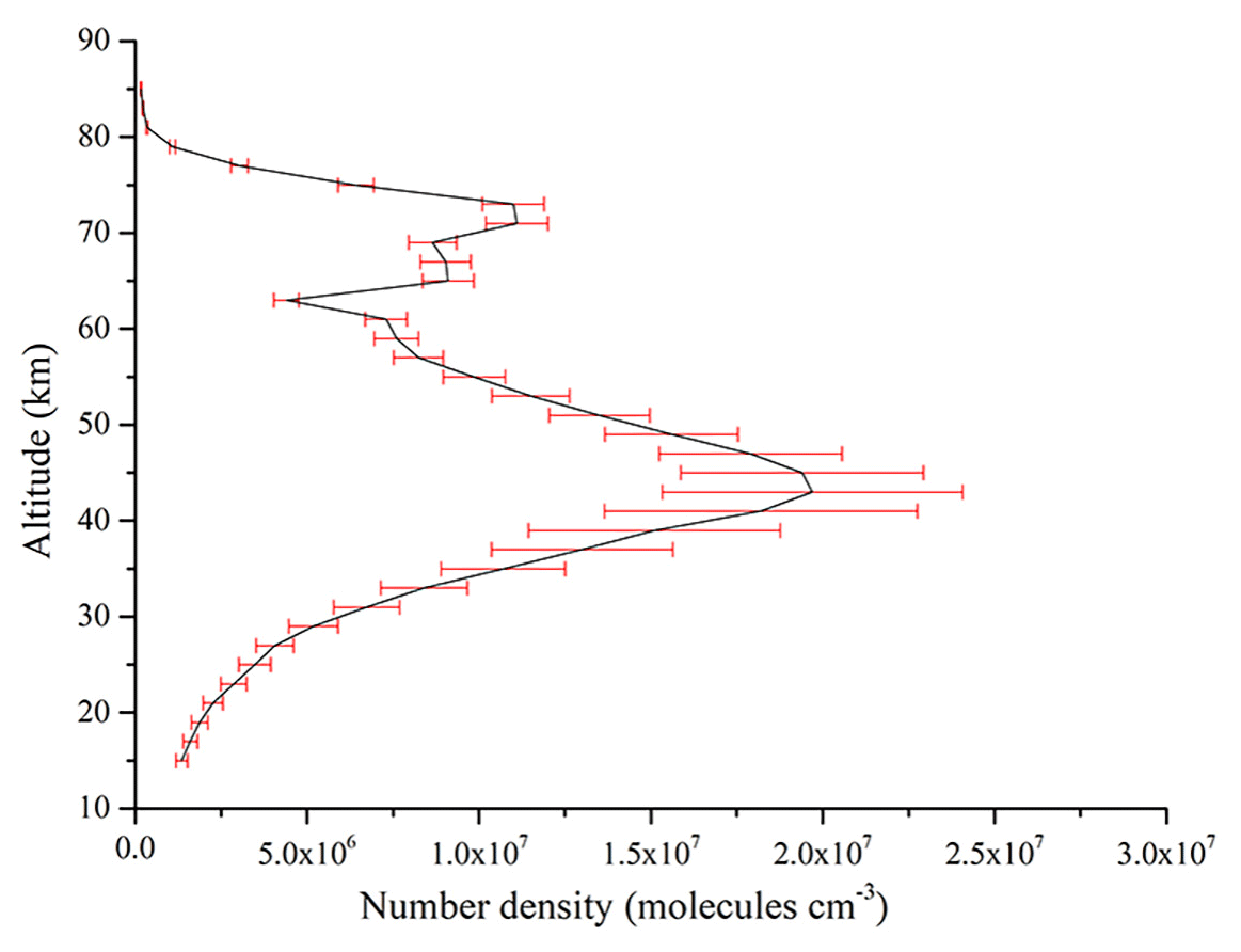
Figure 21Total errors in inversion results caused by some factors mentioned in the text. The red error bars indicate the relative errors caused by some factors mentioned in the text.
Table 8Total errors in inversion results at some tangent heights.
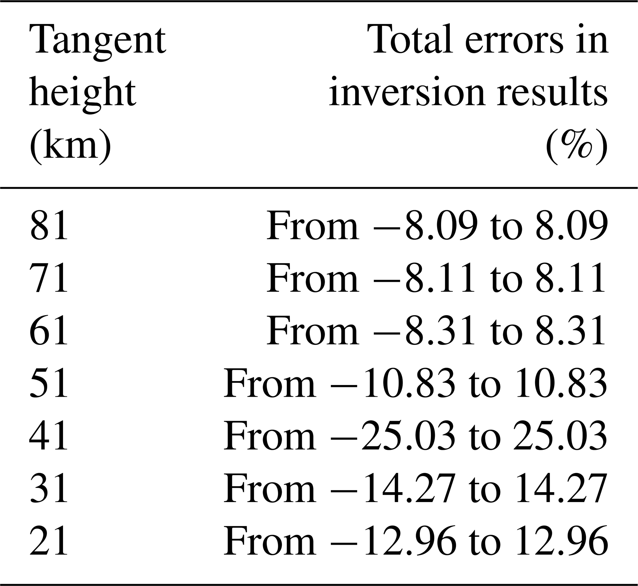
As Table 8 indicates, the total errors in OH concentrations initially increase with the heights rising. They reach the maximum value range from −25.03 % to 25.03 % at 41 km and then decrease from −8.09 % to 8.09 % as the heights continue to rise until reaching the limited height. The total errors in the inversion results in the lower atmosphere are especially small. However, the OH concentrations obtained by the LSUV algorithm in the same area are unsuitable for the scientific research mentioned in Sect. 5.2. A great improvement is evident when compared with the results of the LSUV retrieval algorithm which has a characteristic of iteration. The relative errors of the OH concentrations obtained by the LSUV algorithm are calculated by Eq. (17) and the error transfer formula mentioned above. The initial guess values have a great influence on the iterative speed and the inversion results for the iterative retrieval algorithm. A realistic initial guess value can achieve higher iteration efficiency and more accurate inversion results. The initial guess values used in the LSUV retrieval algorithm are obtained from the OH concentration database through the date parameters and spatial information such as the season, latitude, and longitude of the target area. The corresponding accuracy ranges and useful height ranges of MLS OH concentration products are also given by the MLS data quality and description document (Livesey et al., 2015). Therefore, the data accuracy is assigned at the upper limited height to an altitude greater than the upper limit of the MLS data altitude and at the lower limited height to an altitude smaller than the lower limit of the MLS data altitude. The initial guess values can be obtained by using the data accuracy to perform the positive and negative turbulence processing for the initial OH concentration values. A minimum positive value is given to the data less than zero for the physical meaning when a negative value may occur in the negative direction. The two initial guess values are used in the LSUV retrieval algorithm separately. Although, the initial guess values mentioned above are chosen scientifically and reasonably, the inversion results are unsuitable for scientific research in the lower atmosphere, in which the relative errors caused by the initial guess values reach from −95.39 % to 545.44 %. Besides the initial guess values, the inversion results are also affected by the errors caused by the atmospheric model, the Doppler effect, and the instrument calibration error. The relative errors in inversion results obtained by the LSUV retrieval algorithm are small from 30 to 85 km. The total errors in inversion results are from −24.83 % to 24.83 % at 31 km and then decrease gradually until the altitude of 51 km. A small increase occurs from the altitude of 60 to 70 km and reaches from −37.01 % to 37.01 % at the 81 km. However, the inversion results are poor in the lower atmosphere. The total errors in inversion results are from −553.16 % to 553.16 % at 21 km. The total errors in inversion results are 2 times larger than those obtained by the tomographic retrieval algorithm at some heights like 71 and 61 km. However, the total errors in the inversion results are 4.625 times larger than the errors in the results of the tomographic retrieval algorithm; the difference is especially large at 21 km. The application altitudes of the LSUV retrieval algorithm are limited. The main reasons leading to these unscientific inversion results are twofold. The OH fluorescence emission radiance, the main factor for the retrieval algorithm, is not strong enough due to the ozone optical depth becoming large in the lower atmosphere. That will lead to the observed radiance coming not from the tangent area but from the near field. The lower atmospheric environment is complicated. Human activity will produce a lot of substances which will enter the atmospheric environment by atmospheric convection motion. Aerosols are also distributed here. These will lead to a low accuracy of detection. So the useful altitudes of the LSUV retrieval algorithm based on the data of a single spatial heterodyne spectrometer are limited. The DSHS can counteract the errors by the two spatial heterodyne spectrometers because of its special optical design which the inversion results of the retrieval algorithm have proved. These analyses described above also indicate that the tomographic retrieval algorithm is a feasible retrieval algorithm for the atmosphere from 15 to 85 km. The lookup table method avoids the intervention of initial guess values effectively by establishing a tomographic-observation database of multidimensional variables and is understood easily. It also avoids the complicated iterative optimization process, and the OH concentrations can be obtained directly from the tomographic-observation database. This makes the speed of the inversion process fast compared with the LSUV retrieval algorithm. The tomographic retrieval algorithm is a suitable retrieval algorithm for the three-dimensional limb mode of the DSHS as well. The three-dimensional limb mode provides numerous observed data. The speed of traditional iterative retrieval algorithms is slow and will take a lot of time. However, it is difficult to quantify how fast the tomographic algorithm is absolutely. The traditional iterative retrieval algorithm will take several or even tens of hours to obtain OH concentrations due to the complex iterative process. The tomographic algorithm just needs minutes for obtaining the OH concentrations due to the usage of the lookup table method. The results obtained by the traditional iterative retrieval algorithm in the lower atmosphere are unscientific, but the OH concentrations obtained by the tomographic algorithm in the same area are accurate. The tomographic retrieval algorithm solves these problems described above and improves the efficiency of the retrieval algorithm which is important for the OH concentrations. The LSUV retrieval algorithm can invert OH concentrations well under the conditions that the OH fluorescence emission radiance is strong and the interference factors like water vapor and ozone are small. However, a single spatial heterodyne spectrometer with a traditional limb mode cannot obtain enough high-quality data to invert the OH concentrations, making the inversion results unscientific especially in the lower atmosphere. The initial guess values play a significant role in the LSUV retrieval algorithm due to the feature of the iteration. The determination of the initial guess values involves many factors, and there is no best way to determine the initial guess values at present. This feature is particularly pronounced in the lower atmosphere where OH fluorescence emission radiance is less sensitive to OH concentrations.
In summary, the LSUV retrieval algorithm based on the iterative method can invert the OH concentrations well in the higher atmosphere like the mesosphere but cannot obtain the accurate OH concentrations in the lower atmosphere like the bottom of the stratosphere. Many factors lead to this result like the atmospheric model and the limit of initial guess values. The tomographic retrieval algorithm using the lookup table method can obtain the accurate OH concentrations from the stratosphere to mesopause through the feature of the three-dimensional limb mode. This retrieval algorithm not only saves time in the inversion process but also solves the problem that the OH concentrations are unsuitable for scientific research in the lower atmosphere.
OH is the key oxidant in the atmosphere and has a great influence on the atmospheric photochemistry process. The DSHS based on the spatial heterodyne spectroscopy will monitor the OH with the three-dimensional limb mode in the future. A forward model is constructed to simulate the observed data of the DSHS accurately. A new retrieval algorithm for obtaining the OH concentrations is also proposed based on the simulations of the forward model. The distinctive feature of this algorithm is the usage of a lookup table method. The MLS OH concentration products and N32 Gaussian grid are used to construct the OH concentration database of the four seasons. The observed radiance is obtained by the forward model. The other factors like spatial information and observation geometries are also simulated according to the characteristics of the DSHS for the tomographic retrieval algorithm. The tomographic-observation database is established based on the parameters described above. The OH concentrations in the target area are obtained through searching in the tomographic-observation database directly. The cubic-spline-interpolation method is also used to obtain the OH concentrations without the corresponding query conditions. The errors caused by the atmospheric model, the instrument calibration error, the Doppler effect, and the interpolation algorithm are also analyzed. The results show that the tomographic retrieval algorithm not only is faster compared with the LSUV retrieval algorithm but also improves the inversion precision of the OH concentrations especially in the lower atmosphere.
There are still some problems to be solved when the DSHS is officially in operation in the future. The performances of two spatial heterodyne spectrometers are inevitably different because they are affected by the temperature, humidity, and electromagnetic environment during manufacturing although the biorthogonal structure is theoretically identical in the design parameters. The instrument calibration errors in the instrument are only considered to be 5 % at present. This part will be optimized according to the actual working conditions after the instrument is officially in operation. The actual observed data are the key point for this research. Some aircraft flight experiments have been performed, and the data are being analyzed.
All code and data can be obtained from the corresponding author upon request.
YA and JM designed the study. YA and GB performed the simulations and carried out the data analysis. JM, WX, and XW provided useful comments on the paper. YA prepared the manuscript with contributions from all co-authors.
The authors declare that they have no conflict of interest.
The authors of this study would like to thank the Key Laboratory of Optical Calibration and Characterization of the Chinese Academy of Sciences for funding this research. We also would like to thank Alex Rozanov from the Department of Remote Sensing, Institute of Environmental Physics, University of Bremen, Germany, for helpful advice on using SCIATRAN.
This study was supported by the National Natural Science Foundation of China (grant no. 41671352) and the top-notch university academically funded projects (grant no. gxbjZD06).
This paper was edited by Keding Lu and reviewed by two anonymous referees.
Aruga, T. and Igarashi, T.: Vertical distribution of ozone: a new method of determination using satellite measurements, Appl. Optics, 15, 261–272, https://doi.org/10.1364/AO.15.000261, 1976.
Aruga, T. and Heath, D. F.: An improved method for determining the vertical ozone distribution using satellite measurements, J. Geomagn. Geoelectr., 40, 1339–1363, https://doi.org/10.5636/jgg.40.1339, 1988.
Cageao, R. P., Blavier, J., Mcguire, J. P., Jiang, Y., Nemtchinov, V., Mills, F. P., and Sander, S. P.: High-resolution Fourier-transform ultraviolet–visible spectrometer for the measurement of atmospheric trace species: application to OH, Appl. Optics, 40, 2024–2030, https://doi.org/10.1364/AO.40.002024, 2001.
Cheung, R., Li, K. F., Wang, S., Pongetti, T. J., Cageao, R. P., Sander, S. P., and Yung, Y. L.: Atmospheric hydroxyl radical (OH) abundances from ground-based ultraviolet solar spectra: an improved retrieval method, Appl. Optics, 47, 6277–6284, https://doi.org/10.1364/AO.47.006277, 2008.
Conway, R. R., Stevens, M. H., Brown, C. M., Cardon, J. G., Zasadil, S. E., and Mount, G. H.: Middle Atmosphere High Resolution Spectrograph Investigation, J. Geophys. Res., 104, 16327–16348, https://doi.org/10.1029/1998JD100036, 1999.
Conway, R. R, Summer, M. E., Stevens, M. H., Cardon, J. G., Preusse, P., and Offermann, D.: Satellite Observation of Upper Stratospheric and Mesospheric OH: The HOx Dilemma, Geophys. Res. Lett., 27, 2613–2616, https://doi.org/10.1029/2000GL011698, 2000
Damiani, A., Storini, M., Santee, M. L., and Wang, S.: Variability of the nighttime OH layer and mesospheric ozone at high latitudes during northern winter: influence of meteorology, Atmos. Chem. Phys., 10, 10291–10303, https://doi.org/10.5194/acp-10-10291-2010, 2010.
Dohi, T. and Suzuki, T.: Attainment of High Resolution Holographic Fourier Transform Spectroscopy, Appl. Optics, 10, 1137–1140, https://doi.org/10.1364/AO.10.001137, 1971.
Englert, C. R., Stevens, M. H., Siskind, D. E., Harlander, J. M., Roesler, F. L., and Pickett, H. M., Von Savigny, C., and Kochenash, A. J.: First results from the Spatial Heterodyne Imager for Mesospheric Radicals (SHIMMER): Diurnal variation of mesospheric hydroxyl, Geophys. Res. Lett., 35, L19813, https://doi.org/10.1029/2008GL035420, 2008.
Englert, C. R., Stevens, M. H., Siskind, D. E., Harlander, J. M., and Roesler, F. L.: Spatial Heterodyne Imager for Mesospheric Radicals on STPSat-1, J. Geophys. Res., 115, D20306, https://doi.org/10.1029/2010JD014398, 2010.
Felton, C. C., Sheppard, J. C., and Campbell, M. J.: The radiochemical hydroxyl radical measurement method, Environ. Sci. Technol., 24, 1841–1847, https://doi.org/10.1021/es00082a009, 1990.
Gao, H., Xu, J., Chen, G., Yuan, W., W, S., V, M. A., and V, M. I.: Impact of the Uncertainties of Input Parameters on the Atomic Oxygen Density Derived From OH Nightglow, Chinese J. Space Sci., 29, 304–310, 2009.
Hard, T. M., Obrien, R. J., Chan, C. Y., and Mehrabzadeh, A. A.: Tropospheric free radical determination by FAGE, Environ. Sci. Technol., 18, 768–777, https://doi.org/10.1021/es00128a009, 1984.
Harlander, J. M., Roesler, F. L., Cardon, J. G., Englert, C., and Conway, R. R.: SHIMMER: A Spatial Heterodyne Spectrometer for Remote Sensing of Earth's Middle Atmosphere, Appl. Optics, 41, 1343–1352, https://doi.org/10.1364/AO.41.001343, 2002.
Lelieveld, J., Gromov, S., Pozzer, A., and Taraborrelli, D.: Global tropospheric hydroxyl distribution, budget and reactivity, Atmos. Chem. Phys., 16, 12477–12493, https://doi.org/10.5194/acp-16-12477-2016, 2016.
Livesey, N. J., Van Snyder, W., Read, W. G., and Wagner, P. A.: Retrieval algorithms for the EOS Microwave limb sounder (MLS), IEEE T. Geosci. Remote, 44, 1144–1155, https://doi.org/10.1109/TGRS.2006.872327, 2006.
Livesey, N. J., Read, W. G., Wagner, P. A., Froidevaux, L., Lambert, A., Manney, G. L., Valle, L. F. M., Pumphrey, H. C., Santee, M. L., Schwartz, M. J., Shu-hui W, Fuller, R. A., Jarnot, R. F., Knosp, B. W., and Martinez E.: Version 4.2x Level 2 data quality and description document, Jet Propulsion Laboratory, California, United States of America, 2015.
Lu, K., Guo, S., Tan, Z., Wang, H., Shang, D., Liu, Y., Li, X., Wu, Z., Hu, M., and Zhang, Y.: Exploring the Atmospheric Free Radical chemistry in China: the self-cleansing capacity and the formation of secondary air pollution, Natl. Sci. Rev., 6, 579–594, https://doi.org/10.1093/nsr/nwy073, 2019
Luque, J. and Crosley, D. R.: LIFBASE: Database and Spectral Simulation Program (Version 1.5), SRI International Report MP, 99, 1999.
Mauldin, R. L., Frost, G. J., Chen, G., Tanner, D. J., Prevot, A. S. H., Davis, D. D., and Eisele, F. L.: OH measurements during the First Aerosol Characterization Experiment (ACE 1): Observations and model comparisons, J. Geophys. Res., 103, 16713–16729, https://doi.org/10.1029/98jd00882, 1998.
Mills, F. P., Cageao, R. P., Nemtchinov, V., Jiang, Y., and Sander, S. P.: OH column abundance over Table Mountain Facility, California: Annual average 1997–2000, Geophys. Res. Lett., 29, 32-1–32-4, https://doi.org/10.1029/2001gl014151, 2002.
Perner, D., Ehhalt, D. H., Patz, H. W., Platt, U., Roth, E. P., and Volz, A.: OH – Radicals in the lower troposphere, Geophys. Res. Lett., 3, 466–468, https://doi.org/10.1029/GL003i008p00466, 1976.
Rothman, L. S., Gordon, I. E., Babiov, Y., Barbe, A., Benner, D. C., Bernath, P. E., Birk, M., Bizzocchi, L., Boudon, V., Brown, L. R., Campargue, A., Chance, K., Cohen, E. A., Coudert, L.H., Devi, V. M., Drouin, B. J., Fayt, A., Flaud, J. -M., Gamache, R. R., Harrison, J. J., Hartmann, J.-M., Hill, C., Hodges, J.T., Jacquemart, D., Jolly, A., Lamouroux, J., Roy, L. R. J., Li, G., Long, D.A., Lyulin, O.M., Mackie, C. J., Massi, S. T., Mikhailenko, S., Müller, H. S. P., Naumenko, O. V., Nikitin, A. V., Orphal, J., Perevalov, V., Perrin, A., Polovtseva, E. R., Richard, C., Smith, M. A. H., Starikova, E., Sung, K., Tashkun, S., Tennyson, J., Toon, G. C., Tyuterev, Vl. G., and Wagner, G.: The HITRAN2012 molecular spectroscopic database, J. Quant. Spectrosc. Ra., 130, 4–50, https://doi.org/10.1016/j.jqsrt.2013.07.002, 2013.
Rozanov, V. V., Rozanov, A. V., Kokhanovsky, A. A., and Burrows, J. P.: Radiative transfer through terrestrial atmosphere and ocean: Software package SCIATRAN, J. Quant. Spectrosc. Ra., 133, 13–71, https://doi.org/10.1016/j.jqsrt.2013.07.004, 2014.
Salmon, R. A., Schiller, C. L., and Harris, G. W.: Evaluation of the salicylic acid – Liquid phase scrubbing technique to monitor atmospheric hydroxyl radicals, J. Atmos. Chem., 48, 81–104, https://doi.org/10.1023/b:joch.0000034516.95400.c3, 2004.
Sinnhuber, B.-M., Sheode, N., Sinnhuber, M., Chipperfield, M. P., and Feng, W.: The contribution of anthropogenic bromine emissions to past stratospheric ozone trends: a modelling study, Atmos. Chem. Phys., 9, 2863–2871, https://doi.org/10.5194/acp-9-2863-2009, 2009.
Stevens, P. S., Mather, J. H., and Brune, W. H.: Measurement of tropospheric OH and HO2 by laser-induced fluorescence at low pressure, J. Geophys. Res., 99, 3543–3557, https://doi.org/10.1029/93JD03342, 1994.
Wang, S., Pickett, H. M., Pongetti, T. J., Cheung, R., Yung, Y. L., Shim, C., Li, Q., Canty, T. P., Salawitch, R. J., and Jucks, K. W.: Validation of Aura Microwave Limb Sounder OH measurements with Fourier Transform Ultra-Violet Spectrometer total OH column measurements at Table Mountain, California, J. Geophys. Res., 113, D22301, https://doi.org/10.1029/2008JD009883, 2008.
Watanabe, T., Yoshida, M., Fujiwara, S., Abe, K., Onoe, A., Hirota, M., and Igarashi, S.: Spin trapping of hydroxyl radical in the troposphere for determination by electron spin resonance and gas chromatography/mass spectrometry, Anal. Chem., 54, 2470–2474, https://doi.org/10.1021/ac00251a015, 1982.
Wolfe, G. M., Nicely, J. M., Clair, J. M. S., Hanisco, T. F., Liao, J., Oman, L. D., Brune, W. B., Miller, D. J., Thames, A. B., and Abad, G. G.: Mapping hydroxyl variability throughout the global remote troposphere via synthesis of airborne and satellite formaldehyde observations, P. Natl. Acad. Sci. USA, 116, 11171–11180, https://doi.org/10.1073/pnas.1821661116, 2019.
Ye, S., Xiong, W., Qiao, Y., Hong, J., and Fang, Y.: Data processing for interferogram of spatial heterodyne spectrometer, Spectrosc. Spect. Anal., 29, 848–852, https://doi.org/10.3964/j.issn.1000-0593(2009)03-0848-05, 2009.
Zhang, H., Gao, Y., Li, C., Ma, J., Fang, X., and Xiong, W.: Simulation of Limb Measurements for Mesospheric Hydroxyl Radical Based on SHS Detector, Spectrosc. Spect. Anal., 37, 2685–2691, 2017.
Zhang, Y., Jacob, D. J., Maasakkers, J. D., Sulprizio, M. P., Sheng, J.-X., Gautam, R., and Worden, J.: Monitoring global tropospheric OH concentrations using satellite observations of atmospheric methane, Atmos. Chem. Phys., 18, 15959–15973, https://doi.org/10.5194/acp-18-15959-2018, 2018.