Combined use of Mie–Raman and fluorescence lidar observations for improving aerosol characterization: feasibility experiment

To study the feasibility of a fluorescence lidar for aerosol characterization, the fluorescence channel is added to the LILAS multiwavelength Mie–Raman lidar of Lille University, France. A part of the fluorescence spectrum induced by 355 nm laser radiation is selected by the interference filter of 44 nm bandwidth centered at 466 nm. Such an approach has proved to have high sensitivity, allowing fluorescence signals from weak aerosol layers to be detected and the fluorescence backscattering coefficient from the ratio of fluorescence and nitrogen Raman backscatters to be calculated. Observations were performed during the November 2019–February 2020 period. The fluorescence capacity (ratio of fluorescence to elastic backscattering coefficients), measured under conditions of low relative humidity, varied in a wide range, being the highest for the smoke and the lowest for the dust particles. The results presented also demonstrate that the fluorescence measurements can be used for monitoring the aerosol inside the cloud layers.

1 Introduction

Aerosol–cloud interactions are one of the key factors influencing the Earth radiation balance, and, for its realistic modeling, knowledge of aerosol properties both outside and within the cloud layer is needed. Multiwavelength Mie–Raman lidar and High Spectral Resolution Lidar (HSRL), measuring aerosol backscattering and extinction coefficients at multiple wavelengths, are widely used for the remote characterization of aerosol properties (e.g., Tesche et al., 2011; Burton et al., 2012; Papagiannopoulos et al., 2018; Veselovskii et al., 2020 and references therein). However, although useful for studying aerosol, the amount of information contained in these measurements remains limited (Burton et al., 2016; Alexandrov and Mishchenko, 2017). In addition, such lidars are not able to detect and characterize aerosol inside a cloud layer because aerosol scattering is masked by strong cloud particle scattering. To improve the lidar capability for aerosol characterization, additional channels, measuring the laser-induced fluorescence, can be used. Fluorescence spectroscopy is a highly sensitive technique, widely used for the in situ monitoring of atmospheric organic particles (Pan et al., 2007; Pan, 2015; Miyakawa et al., 2015; Huffman et al., 2020). The synergy of fluorimetry and lidar technology provides an opportunity to perform such monitoring remotely (Immler et al., 2005; Rao et al., 2018; Saito et al., 2018; Li et al., 2019). Numerous types of atmospheric aerosols, such as biological, biomass burning particles, sulfates and even dust, are fluorescent, being excited by UV radiation. When the excitation wavelength is 355 nm, the main part of the emission spectra is usually contained within the 400–650 nm range (Pan, 2015). The fluorescence spectrum varies with aerosol type and composition, therefore making their identification possible. Moreover, due to the fact that pure water does not fluoresce, the measurement of cloud fluorescence allows information to be obtained about aerosol particles within the cloud layer, at least near the cloud base, thus allowing aerosol–cloud coexistence to be investigated.

One of the factors that complicates quantitative information about aerosol properties being obtained from fluorescence measurements is the influence of relative humidity (RH). The aerosol particles grow by water uptake, changing their elastic scatter cross section, but the change in water percentage within an aerosol particle normally does not alter the chemical components, so the total amount of fluorescent molecules within a particle does not change. However the illumination intensity distribution within a particle, as well as the emission angle distribution, will be altered by the change of particle size, shape and refractive index, and this modification may affect the fluorescence measurement. The phase functions of the microspheres for incoherent scattering (fluorescence is an example of incoherent scattering) were computed in works of Kerker and Druger (1979) and Veselovskii et al. (2002a). Results demonstrate that the fluorescence of particles dissolved in water microspheres can be increased in the backward direction by a factor of ∼ 2 compared to the fluorescence of a bulk material (calculated per gram of solid matter). This enhancement, however, occurs for relatively big microspheres, with the size parameter $x=\frac{\mathrm{2}\mathit{\pi }r}{\mathit{\lambda }}$ exceeding approximately 10 (Veselovskii et al., 2002a). For the wavelength λ= 532 nm, the corresponding radius r is about 1.0 µm, so the fluorescence of the fine-mode particles should be affected less by the hygroscopic growth. We should also mention that for insoluble particles, the presence of the water shell, under conditions of high RH, in principle, can lead to an additional increase of the fluorescence, due to the water droplet lens effect. A similar effect is well known for soot particles covered by a non-absorbing shell (Schnaiter, 2005).

Interpretation of fluorescent measurements in a cloud is even more challenging. The liquid cloud is a mixture of interstitial aerosol particles (non-activated particles) and droplets, formed on cloud condensation nuclei (CCN). The CCN may be completely dissolved in the droplets or survived as a solid particle within the droplets, as is the case for dust or soot. The relative contributions of interstitial aerosol and activated CCN in the droplets to the total cloud fluorescence backscatter are unknown, and the need to estimate these contributions was one of the motivations of this study.

The recent interest in fluorescence lidars has also been stimulated by progress in the development of the multianode photomultipliers, allowing for, in combination with spectrometers, the simultaneous detection of the lidar signal in 32 spectral bins (Sugimoto et al., 2012; Reichardt, 2014; Reichardt et al., 2017; Saito et al., 2018). Such multichannel detection has the obvious advantage of analyzing the whole spectrum, allowing for the aerosol identification. However, the sensitivity of such lidar spectrometers is lower when compared to the technique based on the selection of fluorescence spectrum intervals with interference filters because the transmission of modern filters exceeds 90 %. The use of interference filters, in addition to being more sensitive, allows for more affordable modification of a multiwavelength Mie–Raman lidar by adding one or more fluorescence channels. To obtain the highest sensitivity, it is mandatory to acquire the fluorescence in a wide spectral range, which, however, makes the data analysis more complicated because variation of aerosol and molecular transmission within the detection spectral range has to be accounted for. In addition, in Mie–Raman multiwavelength lidars, one should avoid the spectral intervals affected by elastic scattering and corresponding strong Raman lines.

In our paper we present the results of a feasibility experiment and evaluate the sensitivity of a single-channel fluorescence lidar. Measurements were performed at Laboratoire d'Optique Atmosphérique (LOA) during the November 2019–February 2020 period. During that period, the aerosol load was very low, so we were not able to determine the particle properties from multiwavelength observations. The objective was then to estimate the efficiency and added value of the fluorescence channel. We therefore mainly focus on the analysis of the efficiency of fluorescence lidar monitoring of different types of aerosol and on the detection of aerosol particles inside low-level cloud layers.

2 Experimental setup and data analysis

The measurements were performed using the LILAS multiwavelength Mie–Raman lidar, based on a tripled Nd:YAG laser with a 20 Hz repetition rate and pulse energy of 70 mJ at 355 nm. The backscattered light is collected by a 40 cm aperture Newtonian telescope. The system is designed for the simultaneous detection of elastic and Raman backscatters, allowing for the so-called 3β+2α+3δ data configuration, including three particle backscattering (β) and two extinction (α) coefficients along with three depolarization ratios (δ). Description of the system can be found in a recent publication of Hu et al. (2019). The aerosol extinction and backscattering coefficients at 355 and 532 nm were calculated from Mie–Raman observations (Ansmann et al., 1992), while backscattering at 1064 nm was derived by the Klett method (Klett, 1985).

For the experiment described, the system was modified: the water vapor 408 nm Raman filter was replaced by a fluorescence one. The corresponding optical scheme together with the transmission curve of the interference filter in the fluorescence channel are shown in Fig. 1. The nitrogen Raman and fluorescence optical signals are separated by a dichroic mirror: more than 98 % of 387 nm radiation is reflected, and more than 95 % of fluorescence signal is transmitted. For both nitrogen Raman and fluorescence channels, R9880U-01 photomultiplier tubes (PMTs) were used. A part of the wideband fluorescence signal was selected by an Alluxa interference filter centered at 466 nm with 44 nm bandwidth. The filter transmission, at maximum, exceeds 98 %. The operational band was chosen outside of the overtones of O₂ and N₂ vibrational Raman lines. In addition, the transmission of the selected fluorescence filter band matches the maxima of fluorescence of many organic molecules (Saito et al., 2018; Reichardt et al., 2017). The filter provides OD6 suppression outside the transmission band. To increase the suppression, two identical interference filters were used in tandem. For additional rejection of elastic scattering at 355 and 532 nm the two-band notch filter was used. With such a design, we estimate that the total suppression of elastic scattering in the fluorescence channel is above OD14. In this paper, observations were carried out during nighttime only.

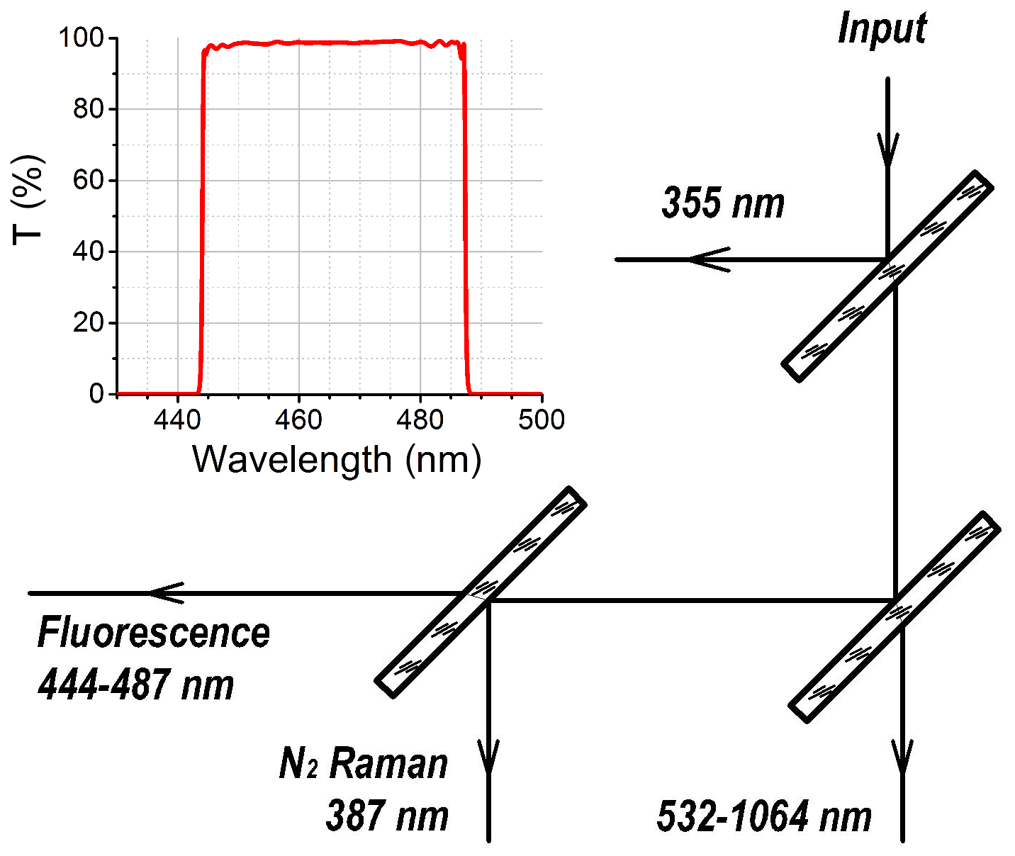
Figure 1 Optical scheme of the elastic, Raman and fluorescence backscatters' separation together with the transmission curve of the interference filter in the fluorescence channel.

In an elastic channel, the backscattered radiative power P_L at distance z is described by the lidar equation

$$\begin{array}{}\text{(1)}& \begin{array}{rl}{P}_{\mathrm{L}}& =O\left(z\right){\displaystyle \frac{\mathrm{1}}{z^{\mathrm{2}}}}{C}_{\mathrm{L}}\left({\mathit{\beta }}_{\mathrm{L}}^{\mathrm{a}}+{\mathit{\beta }}_{\mathrm{L}}^{\mathrm{m}}\right)\exp \left\{-\mathrm{2}\underset{\mathrm{0}}{\overset{z}{\int }}\left({\mathit{\alpha }}_{\mathrm{L}}^{\mathrm{a}}+{\mathit{\alpha }}_{\mathrm{L}}^{\mathrm{m}}\right)\mathrm{d}{z}^{\prime }\right\}\\ & =O\left(z\right){\displaystyle \frac{\mathrm{1}}{z^{\mathrm{2}}}}{C}_{\mathrm{L}}\left({\mathit{\beta }}_{\mathrm{L}}^{\mathrm{a}}+{\mathit{\beta }}_{\mathrm{L}}^{\mathrm{m}}\right)T_{\mathrm{L}}^{\mathrm{2}}.\end{array}\end{array}$$

Here O(z) is the geometrical overlap factor, which is assumed to be the same for elastic, Raman and fluorescence channels. C_L is the range- independent constant, including the efficiency of the detection channel. T_L is the one-way transmission, describing light losses on the way from the lidar to distance z at laser wavelength λ_L. Backscattering and extinction coefficients contain aerosol and molecular contributions, ${\mathit{\beta }}_{\mathrm{L}}^{\mathrm{a}}+{\mathit{\beta }}_{\mathrm{L}}^{\mathrm{m}}$ and ${\mathit{\alpha }}_{\mathrm{L}}^{\mathrm{a}}+{\mathit{\alpha }}_{\mathrm{L}}^{\mathrm{m}}$, where the superscripts “a” and “m” indicate aerosol and molecular scattering, respectively.

In a Raman channel, the backscatter radiative power, P_R , can be rewritten as

$$\begin{array}{}\text{(2)}& \begin{array}{rl}{P}_{\mathrm{R}}& =O\left(z\right){\displaystyle \frac{\mathrm{1}}{z^{\mathrm{2}}}}{C}_{\mathrm{R}}{\mathit{\beta }}_{\mathrm{R}}\exp \left\{-\underset{\mathrm{0}}{\overset{z}{\int }}\left({\mathit{\alpha }}_{\mathrm{L}}^{\mathrm{a}}+{\mathit{\alpha }}_{\mathrm{R}}^{\mathrm{a}}+{\mathit{\alpha }}_{\mathrm{L}}^{\mathrm{m}}+{\mathit{\alpha }}_{\mathrm{R}}^{\mathrm{m}}\right)\mathrm{d}{z}^{\prime }\right\}\\ & =O\left(z\right){\displaystyle \frac{\mathrm{1}}{z^{\mathrm{2}}}}{C}_{\mathrm{R}}{\mathit{\beta }}_{\mathrm{R}}{T}_{\mathrm{L}}{T}_{\mathrm{R}}.\end{array}\end{array}$$

Here T_R is the atmospheric transmission at Raman wavelength λ_R. The Raman backscattering coefficient is

$$\begin{array}{}\text{(3)}& {\mathit{\beta }}_{\mathrm{R}}=N_{\mathrm{R}}{\mathit{\sigma }}_{\mathrm{R}},\end{array}$$

where N_R is the number of Raman scatters (per unit of volume), and σ_R is the Raman differential scattering cross section in the backward direction. To account for the spectral dependence of aerosol extinction, the Ångström exponent γ is used:

$$\begin{array}{}\text{(4)}& {\displaystyle \frac{{\mathit{\alpha }}_{\mathrm{L}}^{\mathrm{a}}}{{\mathit{\alpha }}_{\mathrm{R}}^{\mathrm{a}}}}={\left({\displaystyle \frac{{\mathit{\lambda }}_{\mathrm{R}}}{{\mathit{\lambda }}_{\mathrm{L}}}}\right)}^{\mathit{\gamma }}.\end{array}$$

The aerosol backscattering and extinction coefficients can be computed from Mie–Raman lidar observations using Eqs. (1)–(4), as shown by Ansmann et al. (1992).

In the case of the fluorescence, the emitted wavelengths are spread over a wide spectral range, so the spectral dependence of aerosol and molecular extinction coefficients inside the fluorescence band should be considered. Moreover, the spectral differential fluorescence cross section $\frac{\mathrm{d}{\mathit{\sigma }}_{\mathrm{F}}}{\mathrm{d}\mathit{\lambda }}(\mathit{\lambda },r)$ depends on particle size (Hill, et al., 2015), so the particle size distribution $\frac{\mathrm{d}N\left(r\right)}{\mathrm{d}r}$, which is the number of particles with radii between r and r+dr per unit of volume, has to be considered. The radiative power in the fluorescence channel within the spectral interval [${\mathit{\lambda }}_{min},{\mathit{\lambda }}_{max}$] is

$$\begin{array}{}\text{(5)}& \begin{array}{rl}{P}_{\mathrm{F}}& =O\left(z\right){\displaystyle \frac{\mathrm{1}}{z^{\mathrm{2}}}}{T}_{\mathrm{L}}\underset{{\mathit{\lambda }}_{min}}{\overset{{\mathit{\lambda }}_{max}}{\int }}\underset{r_{min}}{\overset{r_{max}}{\int }}{C}_{\mathrm{F}}\left(\mathit{\lambda }\right)\times {\displaystyle \frac{\mathrm{d}N\left(r\right)}{\mathrm{d}r}}\times {\displaystyle \frac{\mathrm{d}{\mathit{\sigma }}_{\mathrm{F}}}{\mathrm{d}\mathit{\lambda }}}(\mathit{\lambda },r)\\ & \times \exp \left\{-\underset{\mathrm{0}}{\overset{z}{\int }}\left[{\mathit{\alpha }}^{\mathrm{a}}(\mathit{\lambda },z^{\prime })+{\mathit{\alpha }}^{\mathrm{m}}(\mathit{\lambda },z^{\prime })\right]\mathrm{d}{z}^{\prime }\right\}\mathrm{d}r\mathrm{d}\mathit{\lambda }.\end{array}\end{array}$$

The spectral dependence of C_F(λ) is determined mainly by the transmission of the interference filter in the fluorescence channel. If the filter spectral width ${\mathit{\lambda }}_{max}-{\mathit{\lambda }}_{min}$ is not very high, the procedure of data analysis can be simplified. The atmospheric transmission for the fluorescence signal,

$$\begin{array}{}\text{(6)}& T_{\mathrm{F}}\left(\mathit{\lambda }\right)=\exp \left\{-\underset{\mathrm{0}}{\overset{z}{\int }}\left[{\mathit{\alpha }}^{\mathrm{a}}(\mathit{\lambda },z^{\prime })+{\mathit{\alpha }}^{\mathrm{m}}(\mathit{\lambda },z^{\prime })\right]\mathrm{d}{z}^{\prime }\right\},\end{array}$$

can be taken at wavelength λ_F, corresponding to the center of the filter transmission band $T_{\mathrm{F}}\left(\mathit{\lambda }\right)=T_{\mathrm{F}}\left({\mathit{\lambda }}_{\mathrm{F}}\right)\equiv T_{\mathrm{F}}$. The filter transmission used (Fig. 1) is close to rectangular, and sensitivity of the PMT used does not vary significantly within the [${\mathit{\lambda }}_{min},{\mathit{\lambda }}_{max}$] interval, which means the calibration constant C_F can be considered as spectrally independent. Expression (5) can be rewritten by introducing the fluorescence backscattering coefficient β_F:

$$\begin{array}{}\text{(7)}& \begin{array}{rl}\underset{{\mathit{\lambda }}_{min}}{\overset{{\mathit{\lambda }}_{max}}{\int }}& \underset{r_{min}}{\overset{r_{max}}{\int }}{\displaystyle \frac{\mathrm{d}N\left(r\right)}{\mathrm{d}r}}\times {\displaystyle \frac{\mathrm{d}{\mathit{\sigma }}_{\mathrm{F}}}{\mathrm{d}\mathit{\lambda }}}(\mathit{\lambda },r)\mathrm{d}r\mathrm{d}\mathit{\lambda }\\ & =\underset{r_{min}}{\overset{r_{max}}{\int }}{\displaystyle \frac{\mathrm{d}N\left(r\right)}{\mathrm{d}r}}\times {\mathit{\sigma }}_{\mathrm{F}}\left(r\right)\mathrm{d}r={\mathit{\beta }}_{\mathrm{F}}.\end{array}\end{array}$$

Here ${\mathit{\sigma }}_{\mathrm{F}}\left(r\right)=\underset{{\mathit{\lambda }}_{min}}{\overset{{\mathit{\lambda }}_{max}}{\int }}\frac{d{\mathit{\sigma }}_{\mathrm{F}}}{\mathrm{d}\mathit{\lambda }}(\mathit{\lambda },r)\mathrm{d}\mathit{\lambda }$ is the effective fluorescence differential cross section, integrated over the spectral interval [${\mathit{\lambda }}_{min},{\mathit{\lambda }}_{max}$]. The use of β_F allows for Eq. (5) to be rewritten for the power of the fluorescence backscattering similarly to the Raman one.

$$\begin{array}{}\text{(8)}& P_{\mathrm{F}}=O\left(z\right){\displaystyle \frac{\mathrm{1}}{z^{\mathrm{2}}}}{C}_{\mathrm{F}}{\mathit{\beta }}_{\mathrm{F}}{T}_{\mathrm{F}}{T}_{\mathrm{L}}\end{array}$$

The fluorescence backscattering coefficient, β_F, can be obtained from the ratio of Eqs. (8) and (2) for fluorescence and Raman backscatters:

$$\begin{array}{}\text{(9)}& {\mathit{\beta }}_{\mathrm{F}}={\displaystyle \frac{C_{\mathrm{R}}}{C_{\mathrm{F}}}}{\displaystyle \frac{P_{\mathrm{F}}}{P_{\mathrm{R}}}}{N}_{\mathrm{R}}{\mathit{\sigma }}_{\mathrm{R}}{\displaystyle \frac{T_{\mathrm{R}}}{T_{\mathrm{F}}}}.\end{array}$$

The ratio of atmospheric transmissions at λ_R and λ_F wavelengths (T_R∕T_F) can be calculated the same way as for water vapor measurements (Ansmann et al., 1992; Whiteman et al., 2006). In our study, for the nitrogen molecule we used the Raman differential backscattering cross section at 355 nm σ_R = 2.744 × 10⁻³⁰ cm² sr⁻¹ (Venable et al., 2011), but, to obtain absolute values of β_F, the C_R∕C_F ratio must be determined. This ratio can be found from calibration, performed by using a lamp with a known spectrum, as has been done for the Raman water vapor lidars (Venable et al., 2011), but at the current stage, we use a simplified approach for the estimation of C_R∕C_F. The dichroic optics used allows for the efficient separation of fluorescence and Raman signals, so the main source of uncertainty is the relative sensitivity of PMTs in the channels. To equalize sensitivities, the PMT from the fluorescence channel was installed in the Raman one, and by slightly adjusting the voltage, the same value as the nitrogen Raman signal was obtained. The cathode sensitivity of R9880U-01 PMT between 387 and 466 nm changes for less than 15 %; thus we assume that sensitivities of PMTs in both channels are the same, and only the difference in transmission of the interference filters was considered. In all results presented below, a value of $C_{\mathrm{R}}/C_{\mathrm{F}}=\mathrm{0.7}$ was used.

To characterize the efficiency of the fluorescence with respect to elastic scattering, it is convenient to also consider the particle fluorescence capacity,

$$\begin{array}{}\text{(10)}& G_{\mathrm{F}}={\displaystyle \frac{{\mathit{\beta }}_{\mathrm{F}}}{{\mathit{\beta }}_{\mathrm{L}}}},\end{array}$$

which is the ratio of fluorescence and aerosol elastic backscattering coefficients (Reichardt et al., 2017). Here and below, for simplicity, we will use the notation β^a≡β. The aerosol loading in the atmosphere during the experiment was very low, and, in order to decrease the interference of the Raleigh scattering, the backscatter at 1064 nm was mainly used for aerosol characterization, while for the cloud layers the backscattering coefficients at 355 and 532 nm were used as well.

Multiwavelength Mie–Raman lidar measurements allow for the estimation of the particle number density $N=\underset{r_{min}}{\overset{r_{max}}{\int }}\frac{\mathrm{d}N\left(r\right)}{\mathrm{d}r}\mathrm{d}r$ as well as their total volume V (Müller et al., 1999; Veselovskii et al., 2002b); thus a mean fluorescence cross section per single particle can be estimated as ${\mathit{\sigma }}_{\mathrm{F}}^N=\frac{{\mathit{\beta }}_{\mathrm{F}}}{N}$. Assuming that, in the simplest case, a fluorescence backscattering coefficient is proportional to the particle volume, we can estimate the fluorescence cross section per unit of particle volume as ${\mathit{\sigma }}_{\mathrm{F}}^V=\frac{{\mathit{\beta }}_{\mathrm{F}}}{V}$. Thus, the synergy of Mie–Raman and fluorescence lidar measurements should allow for the remote characterization of the particle fluorescent properties. We should mention, however, that estimation of ${\mathit{\sigma }}_{\mathrm{F}}^V$ makes sense only at low RH because water uptake by the particles will alter results.

3 Observation results

3.1 Fluorescence of aerosol layers

The measurements reported were performed during the November 2019–February 2020 period at the Lille Atmospheric Observation Platform (https://www-loa.univ-lille1.fr/observations/plateformes.html?p=apropos, last access: 30 November 2020), hosted by Laboratoire d'Optique Atmosphérique, University of Lille, Hauts-de-France region. Two examples of measurement are presented in Fig. 2 and show height–time distributions of the range-corrected lidar signal (RCLS) at 1064 nm, of the fluorescence backscattering coefficient (β_F) and of the volume depolarization ratio (δ₁₀₆₄), for the nights 29–30 November 2019 and 6–7 February 2020.

Figure 2 The range-corrected lidar signal at 1064 nm, fluorescence backscattering and volume depolarization ratio δ₁₀₆₄ measured at Lille on 29–30 November 2019 (a–c) and 6–7 February 2020 (d–f).

During the first night (left column in Fig. 2), the aerosol layer is localized mainly below 2000 m. Though the aerosol loading is low above 2000 m (β₁₀₆₄ < 0.01 Mm⁻¹ sr⁻¹), it is revealed well by the enhanced depolarization ratio and the enhanced fluorescence backscattering coefficient. During the second night of observation (right column in Fig. 2), a detached/isolated layer is observed at approximately 3000 m. This layer is characterized by a high depolarization ratio (the particle depolarization ratio at 1064 nm in the center of the layer exceeds 15 %), indicating the presence of dust. An explanation of the observed increase of fluorescence signal could be mixing of mineral dust particles with organic materials (Sugimoto et al., 2012; Miyakawa et al., 2015) and local aerosol during transportation.

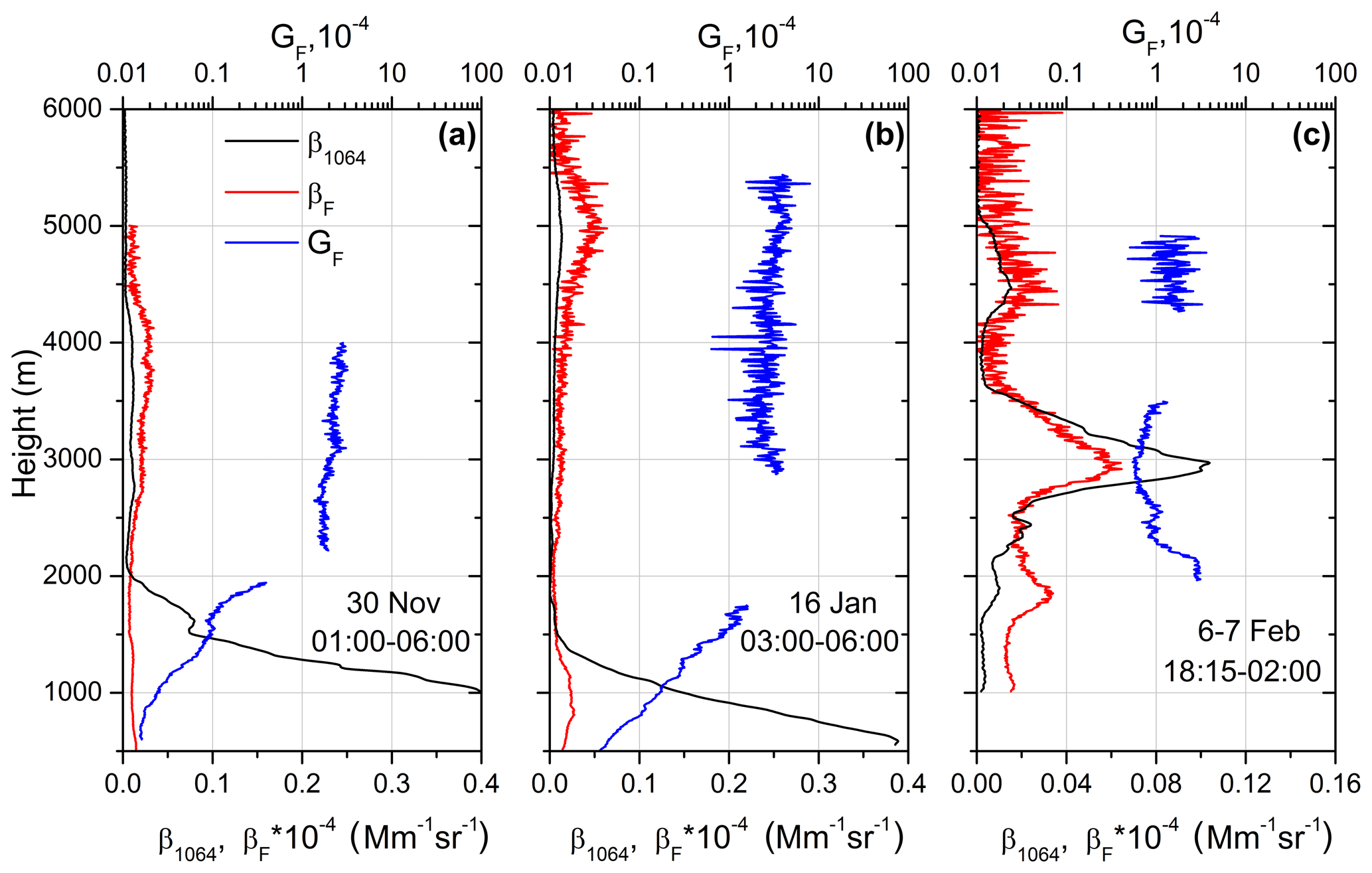
Figure 3 Vertical profiles of aerosol (β₁₀₆₄) and fluorescence (β_F) backscattering coefficients together with the fluorescence capacity (G_F) on (a) 30 November 2019, (b) 16 January 2020 and (c) 6–7 February 2020.

The time-averaged profiles (β₁₀₆₄, β_F, G_F) for these two nights, as well as for the 16 January episode, are shown in Fig. 3. The backscattering coefficient β₁₀₆₄ was calculated by the Klett method, assuming a lidar ratio S = 50 sr. Due to a low aerosol extinction value, the results are not sensitive to the choice of S. The HYSPLIT back trajectory analysis (Stein et al., 2015) demonstrates that on 30 November and 16 January the air masses, at 3500 and 5000 m height respectively, were transported from Canada so could contain biomass burning particles, while on 6–7 February, the air masses at 3000 m arrived from the southwest passing near Africa, thus containing dust particles. The closest available radiosonde data are from the Herstmonceux (UK) and Ebbe (Belgium) stations, located 150 and 95 km away from the observation site respectively. Data from both stations show that on the night 29–30 November 2019 the relative humidity (RH) was about 70 % at 1000 m and dropped below 20 % above 2000 m. The fine mode of the particle size distribution over the observation site is normally predominant inside the planetary boundary layer (PBL). Pure water does not fluoresce, so the water uptake by the fine particles under conditions of high RH is expected to yield an increase of elastic scattering without a significant effect on the fluorescence emission. The aerosol backscattering β₁₀₆₄ on 30 November (Fig. 3a) is 0.4 Mm⁻¹ sr⁻¹ at 1000 m and decreases by a factor of 40 at 1900 m, while β_F within this height range changes less than twice. This supports the assumption that the observed variation of aerosol backscattering in the PBL is mainly due to the change of the particle water fraction. The water uptake at low altitudes agrees with low values of the observed particle depolarization ratio ${\mathit{\delta }}_{\mathrm{1064}}^{\mathrm{p}}$, which is below 0.5 % at 1000 m. Within the weak aerosol layer at the range 2500–4000 m, the particle depolarization ${\mathit{\delta }}_{\mathrm{1064}}^{\mathrm{p}}$ is about 5 %, and we observe an increase of fluorescence capacity G_F, with respect to the layer below 2000 m, of up to 2.5 × 10⁻⁴. This increase of G_F in the 2500–4000 m layer could be due to the presence of another particle type, for example, biomass burning. From this episode, one can conclude that fluorescence backscattering, though being almost 4 orders lower than the elastic one, can be reliably detected with our current lidar configuration.

On 16 January (Fig. 3b), atmospheric RH also decreases with height, from about 80 % at 1000 m to less than 20 % above 2000 m, leading to an increase of G_F for more than 1 order of magnitude. Such variation of G_F within the PBL is probably also related to the particle water uptake, just like in Fig. 3a. Aerosol backscattering increases above 3000 m and reaches its maximum value at 5000 m. Within the 3000–5500 m range, the fluorescence capacity was about 2.5 × 10⁻⁴, which is higher than in the PBL.

On 6–7 February the aerosol loading in the PBL is very low (β₁₀₆₄ < 0.003 Mm⁻¹ sr⁻¹ at 1000 m), and RH from the radiosonde at Herstmonceux is below 40 % in the height range considered. At 3000 m, a dust layer is observed (Fig. 3c). In the middle of this layer, the fluorescence capacity is about 0.6 × 10⁻⁴, which is about a factor of 4 lower than in the elevated layers in Fig. 3a and b. Still, a significant value of G_F can indicate the presence of organic materials in the dust layer (Sugimoto et al., 2012).

Table 1 Parameters of the biomass burning (BB), URban and DUst particles used in the model. The volume V^N=1 and backscattering coefficient ${\mathit{\beta }}_{\mathrm{1064}}^{N=\mathrm{1}}$ are given for a single particle (N=1).

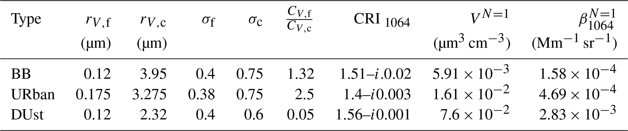
As discussed in Sect. 2, lidar measurements provide an opportunity to estimate the particle fluorescence cross section. For this, we need to know the particle number N and volume V density in the aerosol layer, which, in principle, can be determined from the multiwavelength lidar observations (Muller et al., 1999; Veselovskii et al., 2002b). In our case, however, due to very low aerosol loading, the extinction coefficients could not be determined. Still, the rough estimations of the particle parameters can be done using the predefined aerosol model driven by only a few parameters. In our study we use a simplified approach, modeling aerosol as an external mixture of several aerosol components with predetermined properties. The definition of aerosol components is based on global multiyear AERONET observations (Dubovik et al., 2002) with some modifications. All aerosol types are described by a bimodal particle size distribution (PSD):

$$\begin{array}{}\text{(11)}& {\displaystyle \frac{\mathrm{d}V}{\mathrm{d}\ln r}}=\sum _{i=\mathrm{f},\mathrm{c}}^{\frac{C_{V,i}}{\sqrt{\mathrm{2}\mathit{\pi }}{\mathit{\sigma }}_i}}\exp \left[-{\displaystyle \frac{{\left(\ln r-\ln r_{V,i}\right)}^{\mathrm{2}}}{\mathrm{2}{\mathit{\sigma }}_i^{\mathrm{2}}}}\right],\end{array}$$

where C_V,i denotes the particle volume concentration, r_V,i is the median radius and σ_i is the standard deviation. Subscripts f and c correspond to the fine and coarse mode respectively. The parameters of the number size distribution $\frac{\mathrm{d}N}{\mathrm{d}\ln r}$ can be obtained from Eq. (11) using the expressions from Horvath et al. (1990). Table 1 shows the model parameters for three aerosol types: biomass burning (BB), urban (UR) and dust (DU). From this model, the aerosol backscattering and extinction coefficients can be calculated at any wavelength. As mentioned above, due to low aerosol loading, we only use the backscattering coefficient at 1064 nm, so Table 1 presents ${\mathit{\beta }}_{\mathrm{1064}}^{N=\mathrm{1}}=\frac{{\mathit{\beta }}_{\mathrm{1064}}}{\underset{r_{min}}{\overset{r_{max}}{\int }}\frac{\mathrm{d}N\left(r\right)}{\mathrm{d}r}\mathrm{d}r}$, the mean backscattering coefficient for a single particle (N=1), together with the corresponding complex refractive index (CRI) used in computations. Calculations were performed with assumptions of spherical particles for BB and UR and for the randomly oriented spheroids for dust (Dubovik, et al., 2006). The volume V^N=1 in Table 1 is also given for N=1 (so can be considered as a single particle average volume). Thus, if the aerosol type is known, comparing computed ${\mathit{\beta }}_{\mathrm{1064}}^{N=\mathrm{1}}$ from Table 1 with observed values β₁₀₆₄ yields number and volume particle densities of $N=\frac{{\mathit{\beta }}_{\mathrm{1064}}}{{\mathit{\beta }}_{\mathrm{1064}}^{N=\mathrm{1}}}$ and $V=N\times V^{N=\mathrm{1}}$.

Table 2 The aerosol parameters in elevated layers for three measurement sessions from Fig. 3, including the fluorescence β_F and aerosol β₁₀₆₄ backscattering coefficients, number N and volume V particle densities, the differential fluorescence cross sections per single particle $\frac{{\mathit{\sigma }}_{\mathrm{F}}}{N}$ and per unit of volume $\frac{{\mathit{\sigma }}_{\mathrm{F}}}{V}$, together with spectral density $\frac{{\mathit{\sigma }}_{\mathrm{F}}}{V\mathrm{\Delta }\mathit{\lambda }}$.

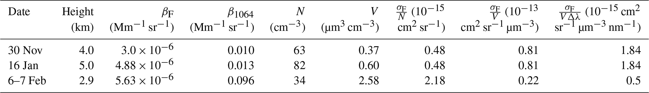
Table 2 summarizes for the 3 nights from Fig. 3 the fluorescence cross sections per single particle, ${\mathit{\sigma }}_{\mathrm{F}}^N=\frac{{\mathit{\beta }}_{\mathrm{F}}}{N}$, and per unit of volume, ${\mathit{\sigma }}_{\mathrm{F}}^V=\frac{{\mathit{\beta }}_{\mathrm{F}}}{V}$. Values are provided for the altitudes corresponding to the maximum of fluorescence backscattering β_F in elevated layers, where the relative humidity (RH) should be low and hygroscopic effect reduced. Based on the back trajectory analysis, particles are assumed to be of biomass burning origin for 30 November and 16 January and of dust origin for 6–7 February. We should reemphasize, however, that our estimations of N (and so ${\mathit{\sigma }}_{\mathrm{F}}^N$) depend on the assumed aerosol type. The particle volume, V, is however a more reliable parameter. For example, if the UR aerosol type is considered, rather than the BB one, the particle number density, N, for 30 November becomes N = 21 cm⁻³ (instead 63 cm⁻³ for BB), while the total volume remains rather constant (V = 0.34 µm³ cm⁻³ instead of 0.37 µm³ cm⁻³). Thus, the presentation of a cross section per unit of volume ${\mathit{\sigma }}_{\mathrm{F}}^V$ appears more trustable. We should also recall that comparison of ${\mathit{\sigma }}_{\mathrm{F}}^V$ for different aerosol types only makes sense at low RH, when the water uptake effect is small. The results in Table 2 are given for the heights, where RH is below 20 %. The fluorescence cross sections ${\mathit{\sigma }}_{\mathrm{F}}^V$ for 30 November and 16 January are very close, but for the dust layer (6–7 February 2020), the cross section is about a factor of 4 lower. From the data presented it is also possible to estimate the spectral differential cross section, $\frac{{\mathit{\sigma }}_{\mathrm{F}}^V}{\mathrm{\Delta }\mathit{\lambda }}$, where Δλ is the width of the filter transmission band.

It is rather difficult to validate our values of the fluorescence differential cross section. We nevertheless compare them to in situ ground-based fluorescence measurements. Such reference data are available mainly for biological particles (e.g., Pan, 2015). For biological particles, the highest $\frac{\mathrm{d}{\mathit{\sigma }}_{\mathrm{F}}}{\mathrm{d}\mathit{\lambda }}$ value for a single particle with diameter 1.2–3.0 µm varies in the range (1–100) × 10⁻¹⁵ cm² sr⁻¹ nm⁻¹ when stimulating radiation at 365 nm is used (Pan, 2015). Thus, our estimated values look reasonable, keeping in mind that the fluorescence cross section of the biological particles is higher than that of smoke. Still, the results presented in the Table 2 should be considered as qualitative, and for obtaining quantitative values, further studies are needed.

3.2 Fluorescence of aerosol particles within cloud layers

One of the attractive features of the fluorescence technique is the possibility to detect aerosol and derive its content within the cloud layer. However the interpretation of fluorescence measurements in the clouds is rather complicated. Aerosol can be inside the cloud droplets in a dissolved or solid state (activated CCN) or in the form of interstitial particles at 100 % RH, and we somehow need to separate their contribution to the fluorescence signal. The fluorescence backscattering β_F is calculated from the ratio of fluorescence and nitrogen Raman lidar signals, and it can be affected by the multiple scattering effects due to significant wavelength separation between Raman and fluorescence components. Thus the most trustable observations should be near the cloud base.

The results of measurements in the presence of thin cloud layers on 13 and 18 November are shown in Fig. 4. The backscattering coefficients are given at 532 nm because in the cloud layers the detector in the 1064 nm channel was sometimes saturated. On 13 November, the cloud layers led to a strong oscillation of β₅₃₂ within the 1000–3000 m range. The spikes in the β₅₃₂ profile, however, are not followed by a synchronous increase of the fluorescence backscattering β_F in the range of 1000–3000 m. On 18 November, the cloud layer within the 1500–2000 m range exhibits an even stronger elastic backscattering, exceeding 80 Mm⁻¹ sr⁻¹, and again, no significant change of fluorescence backscattering is observed. Thus observations in Fig. 4 do not reveal unambiguous effects of cloud layers on aerosol fluorescence. Moreover, these results clearly indicate the absence of leaks or contamination of elastic scattering in the fluorescence channel.

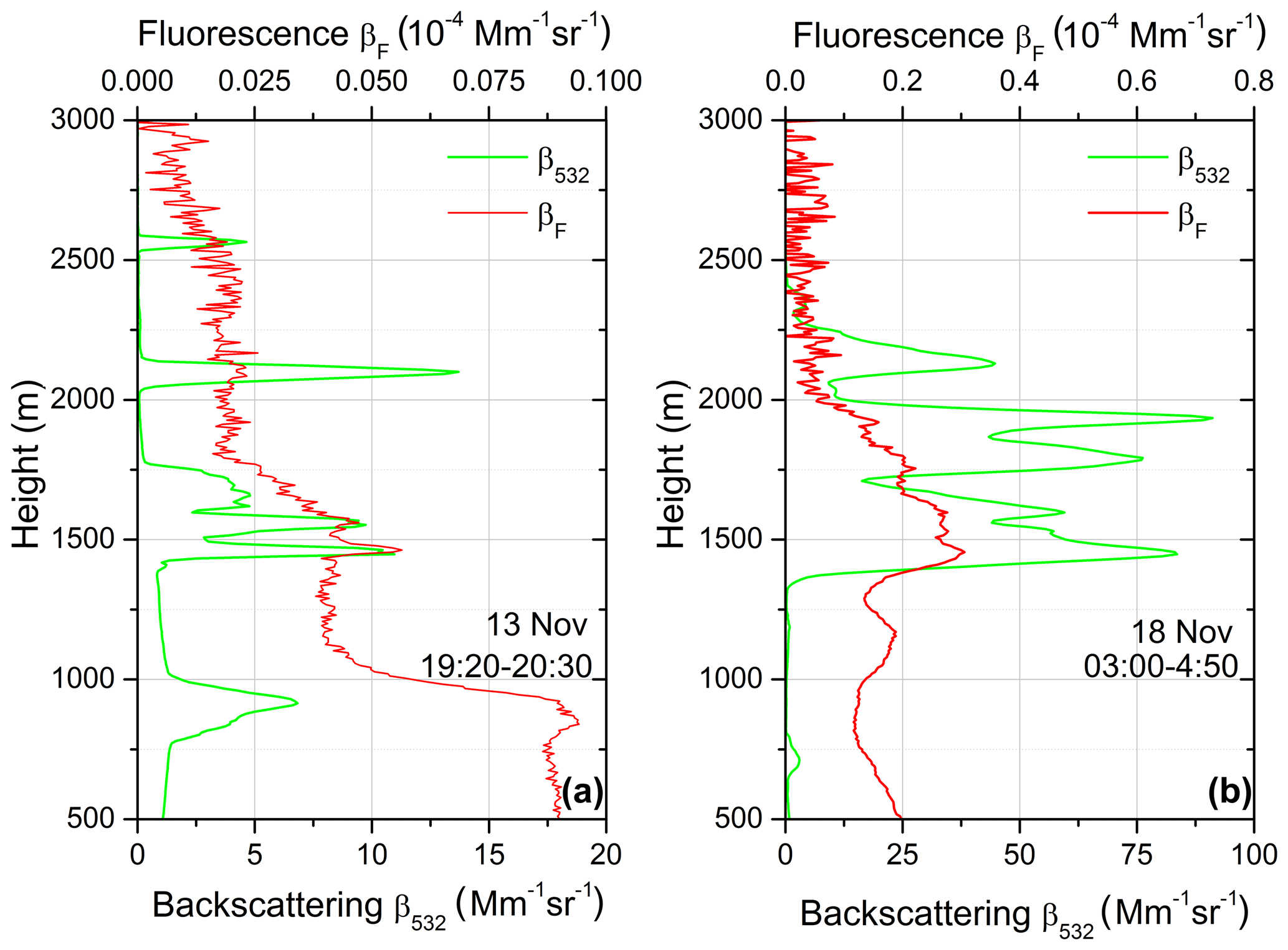
Figure 4 Aerosol (β₅₃₂) and fluorescence (β_F) backscattering coefficients on 13 and 18 November 2019.

The situation, however, can be different when the cloud droplets are formed on the aerosol particles. Figure 5 shows the height–time distributions of the lidar signal at 1064 nm and the fluorescence backscattering coefficient on the night 19–20 November 2019. After 21:50 UTC a thin cloud layer starts to form at the top of the PBL, resulting in a simultaneous increase of β_F. To quantify the influence of cloud water droplets on the fluorescence backscattering, Fig. 6a provides profiles of aerosol and fluorescence backscattering coefficients for two temporal intervals, 20:00–21:30 and 21:30–00:30 UTC, prior to and after the cloud layer formation respectively. Prior to cloud formation, the aerosol load is very low, so backscattering is provided only at 1064 nm, and to be distinguishable in the figure, the value of β₁₀₆₄ is multiplied by a factor of 100. For 20:00–21:30 UTC β₁₀₆₄ at 1500 m (height where the cloud forms) is about 0.07 Mm⁻¹ sr⁻¹. The corresponding value at 532 nm should be about 0.15 Mm⁻¹ sr⁻¹ (for a backscattering Ångström exponent of 1.0). After the cloud formation the backscattering coefficient is shown at 532 nm because the 1064 nm detector in the cloud layer was overloaded. The β₅₃₂ at 1500 m is 500 Mm⁻¹ sr⁻¹; thus β₅₃₂ increases by roughly a factor of 3000, while β_F increases by approximately a factor of 5.

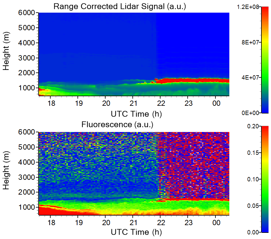
Figure 5 Height–time distribution of the range-corrected lidar signal at 1064 nm and fluorescence backscattering coefficient β_F (in arbitrary units) on 19–20 November 2019.

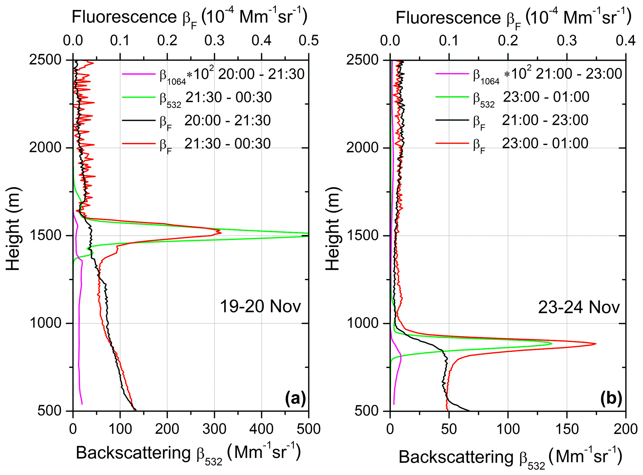
Figure 6 Aerosol and fluorescence backscattering coefficients on (a) 19–20 and (b) 23–24 November 2019 for two time intervals: prior to and after cloud formation. Backscattering coefficient β₁₀₆₄ prior to cloud formation is low, so it is multiplied by a factor of 100 to be distinguishable in this figure.

A similar scenario occurred on the night 23–24 November 2019 (Fig. 6b). Prior to the cloud formation (21:00–23:00 UTC), the backscattering coefficient at 900 m height is β₁₀₆₄ = 0.02 Mm⁻¹ sr⁻¹ (β₅₃₂ should be about 0.02 Mm⁻¹ sr⁻¹), and after cloud formation β₅₃₂ increases up to 130 Mm⁻¹ sr⁻¹. Thus β₅₃₂ enhancement is by a factor of 6500, while β_F again increases by about a factor of 5. The profiles of β_F in Fig. 6 prior to and after the cloud formation remain the same below the cloud. This corroborates the suggestion that the cloud was not transported by the air masses with different properties but that the process of water vapor condensation occurs.

We should emphasize that the enhancement of β_F can not be explained by just insufficient suppression of elastic scattering. The enhancement was observed only inside an aerosol layer, while clouds with similar backscattering coefficients, but outside the aerosol layer, did not provide the increase of β₅₃₂. As mentioned above, the fluorescence scattering phase function of water microspheres can have a peak in the backward direction (Veselovskii et al., 2002a), leading to an increase of β_F, for a particle dissolved in a droplet, by approximately a factor of 2 compared to a solid particle. This is lower than the observed value, and at the moment we are not capable to identify the mechanisms responsible for the β_F enhancement. It should just be mentioned that, in principle, the water environment may affect the fluorescence efficiency. For example, the fluorescence cross section of wet bacterial spores is higher than that of dry ones (Kunnil et al., 2004). For insoluble particles, the presence of a water shell can also lead to an additional increase of the fluorescence due to the lens effect produced by the droplet. More studies are needed to understand the influence of the water uptake by the particles during cloud formation on the fluorescence backscattering.

One of the objectives of this study was to demonstrate the possibility of monitoring aerosol within a cloud by fluorescence. Figure 7 shows the height–time distributions of the range-corrected lidar signal at 1064 nm and the fluorescence backscattering β_F on 15 November 2019 for the 02:45–06:15 UTC period. A low cloud layer appears at approximately 2000 m, and a signal of aerosol fluorescence is observed within this layer up to 3000 m. The HYSPLIT back trajectory analysis shows that air masses at this height are transported over the Atlantic from Canada. The vertical profiles of β₅₃₂ and β_F, integrated over the 02:45–06:15 UTC temporal interval, are shown in Fig. 8a. Fluorescence backscattering is about 0.03 × 10⁻⁴ Mm⁻¹ sr⁻¹ at 1500 m, and it rises to 0.045 × 10⁻⁴ Mm⁻¹ sr⁻¹ at 2000 m, near the cloud base, where RH can be close to 100 %. Inside the cloud β_F increases up to 0.07 × 10⁻⁴ Mm⁻¹ sr⁻¹ at 3000 m, where elastic backscattering is maximal. Thus the total increase of β_F in the 1500–3000 m range is slightly above a factor of 2 and probably can be attributed to the water uptake by the particles. The high value of β_F in the cloud is probably due to the contribution of interstitial aerosol particles.

Figure 7 Height–time distribution of the range-corrected lidar signal (RCLS) at 1064 nm and the fluorescence backscattering coefficient on 15 November 2019.

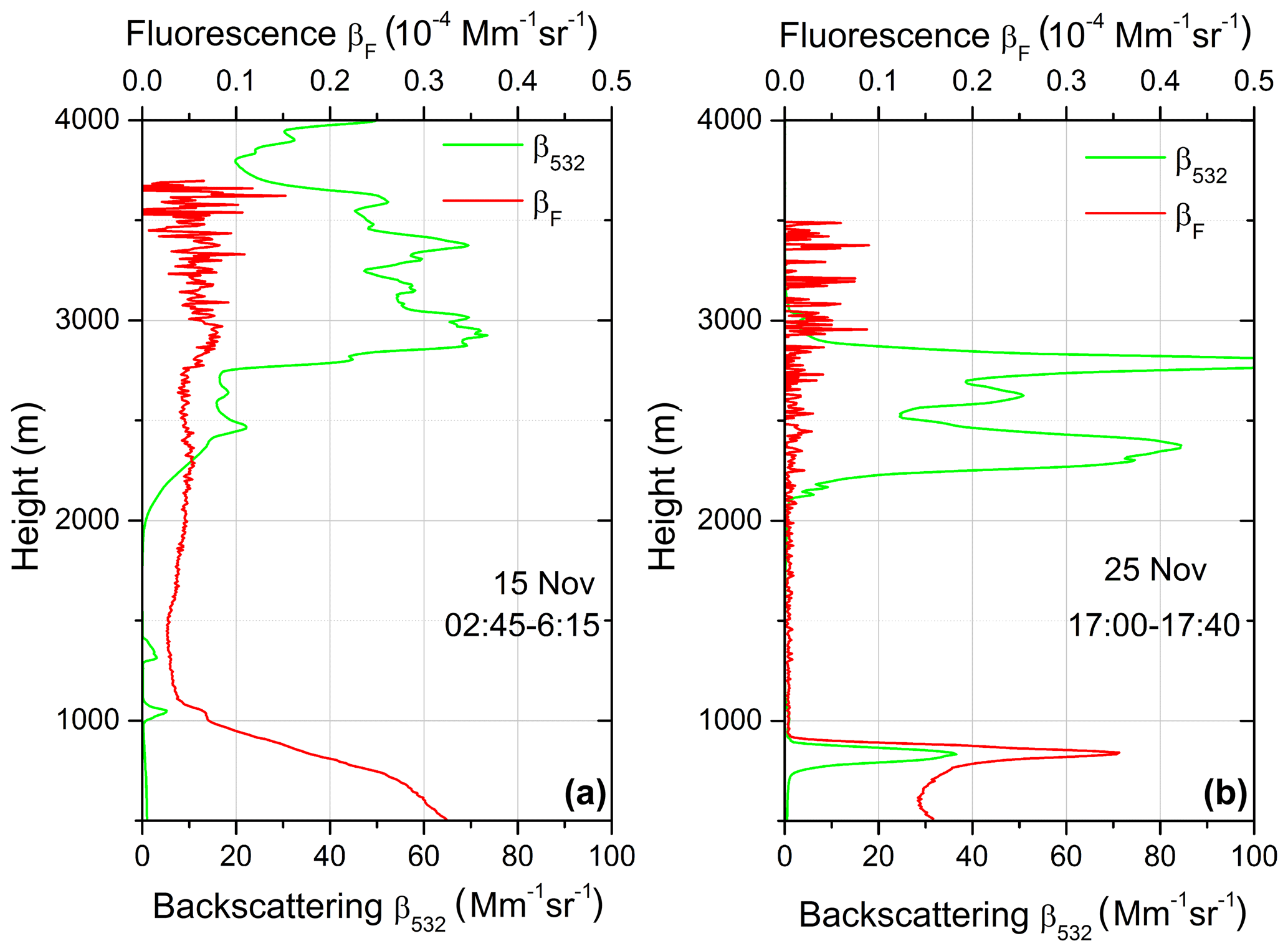
Figure 8 Aerosol (β₅₃₂) and fluorescence (β_F) backscattering coefficients on (a) 15 and (b) 25 November 2019.

On 25 November 2019 (Fig. 8b), a low cloud layer at 850 m leads to an increase of β_F by approximately a factor of 2, in a similar way as in Fig. 6. However, above 1000 m the aerosol content is very low, and β_F is below 0.005 × 10⁻⁴ Mm⁻¹ sr⁻¹. The sensitivity of the fluorescence measurements could be limited by the fluorescence of the optics in the lidar receiver. The lowest value of β_F observed in our measurements (averaged over several hundred meters' height range) was about 0.004 × 10⁻⁴ Mm⁻¹ sr⁻¹; thus β_F in Fig. 8b can be below the limit of our sensitivity. Above 2000 m, a strong cloud layer, with a maximal value of β₅₃₂ above 100 Mm⁻¹ sr⁻¹, occurs. Back trajectory analysis demonstrates that air masses at this height are transported over the Atlantic from the south of the United States. The β_F in the cloud, averaged over the 2200–2750 m range, is about 0.006 × 10⁻⁴ Mm⁻¹ sr⁻¹, which is significantly lower than in Fig. 8a. Thus on 25 November the cloud is less “polluted” by aerosol than on 15 November. The fluorescence signal can be produced by both activated CCN and by interstitial aerosol particle, and at the present stage we are not able to separate their contributions.

4 Conclusion

In our research we analyzed the feasibility of the fluorescence channel, added to the multiwavelength Mie–Raman lidar, for aerosol characterization. The results obtained demonstrate that the use of an interference filter for selection of the part of the fluorescence spectrum allows for efficient lidar operation. In particular, the LILAS lidar with the interference filter of 44 nm width in the fluorescence channel was able to detect the fluorescence signal from weak aerosol layers (β₁₀₆₄ < 0.02 Mm⁻¹ sr⁻¹) up to 5000 m. During the experiment the fluorescence capacity $G_{\mathrm{F}}=\frac{{\mathit{\beta }}_{\mathrm{F}}}{{\mathit{\beta }}_{\mathrm{1064}}}$ of aerosol under conditions of low RH varied through the (0.6–2.5) × 10⁻⁴ range, being the highest for the smoke and the lowest for the dust particles.

The lidar measurements, in principle, allow information to be obtained about the aerosol fluorescence cross section in the elevated aerosol layers. For several atmospheric situations, the rough estimations of the fluorescence cross section were performed in this study, and the results obtained look reasonable compared with published values for biological particles. Still, these results should be taken as preliminary, and the next important step in quantification of the fluorescence measurements will be the system calibration, using a lamp with a known spectrum. In addition, a more detailed comparison of σ_F obtained from the laboratory and lidar measurements, for different aerosol types, is needed for validation. The fluorescence and multiwavelength Mie–Raman lidar techniques are complementary: the multiwavelength lidar allows for aerosol typing and estimation of the particle number and volume densities that are later used to derive the fluorescence cross sections from observed β_F. The fluorescence measurements, in turn, help to improve the aerosol classification. The synergy of fluorescence and multiwavelength lidar techniques was not realized in this study, due to aerosol loading being too low in the November–February period. However, we plan new experiments during spring–summer season, when aerosol optical depth (AOD) is larger in Lille.

Results presented also demonstrate that the fluorescence technique can be used to monitor the aerosol particles inside the cloud (at least near the cloud base, if penetration depth of the laser radiation is small), which is important in the study of aerosol–cloud interaction. However, to get quantitative information about particle properties, we need a deeper understanding of the influence of the water uptake by the particles on the fluorescence efficiency. In particular, in the clouds formed at the top or inside the aerosol layer, an increase of the fluorescence backscattering coefficient up to a factor of 5 was observed, and at the moment we are not able to specify the processes behind this enhancement.

In coming studies we plan additional modifications of the lidar. In particular, we consider the possibility of adding a second fluorescence channel near 550 nm, which should improve selectivity of the fluorescence technique for different aerosol types. The water vapor channel will be returned back to the system, which is essential for the study of particle hygroscopic growth. Collocated measurements of the microwave radiometer of the Laboratoire d'Optique Atmosphérique will be used to derive the RH profiles.