the Creative Commons Attribution 4.0 License.
the Creative Commons Attribution 4.0 License.
 | 15 Dec 2020
Quantifying CO2 emissions of a city with the Copernicus Anthropogenic CO2 Monitoring satellite mission
Grégoire Broquet
Yasjka Meijer
We investigate the potential of the Copernicus Anthropogenic Carbon Dioxide (CO2) Monitoring (CO2M) mission, a proposed constellation of CO2 imaging satellites, to estimate the CO2 emissions of a city on the example of Berlin, the capital of Germany. On average, Berlin emits about 20 Mt CO2 yr−1 during satellite overpass (11:30 LT). The study uses synthetic satellite observations of a constellation of up to six satellites generated from 1 year of high-resolution atmospheric transport simulations. The emissions were estimated by (1) an analytical atmospheric inversion applied to the plume of Berlin simulated by the same model that was used to generate the synthetic observations and (2) a mass-balance approach that estimates the CO2 flux through multiple cross sections of the city plume detected by a plume detection algorithm. The plume was either detected from CO2 observations alone or from additional nitrogen dioxide (NO2) observations on the same platform. The two approaches were set up to span the range between (i) the optimistic assumption of a perfect transport model that provides an accurate prediction of plume location and CO2 background and (ii) the pessimistic assumption that plume location and background can only be determined reliably from the satellite observations. Often unfavorable meteorological conditions allowed us to successfully apply the analytical inversion to only 11 out of 61 overpasses per satellite per year on average. From a single overpass, the instantaneous emissions of Berlin could be estimated with an average precision of 3.0 to 4.2 Mt yr−1 (15 %–21 % of emissions during overpass) depending on the assumed instrument noise ranging from 0.5 to 1.0 ppm. Applying the mass-balance approach required the detection of a sufficiently large plume, which on average was only possible on three overpasses per satellite per year when using CO2 observations for plume detection. This number doubled to six estimates when the plumes were detected from NO2 observations due to the better signal-to-noise ratio and lower sensitivity to clouds of the measurements. Compared to the analytical inversion, the mass-balance approach had a lower precision ranging from 8.1 to 10.7 Mt yr−1 (40 % to 53 %), because it is affected by additional uncertainties introduced by the estimation of the location of the plume, the CO2 background field, and the wind speed within the plume. These uncertainties also resulted in systematic biases, especially without the NO2 observations. An additional source of bias was non-separable fluxes from outside of Berlin. Annual emissions were estimated by fitting a low-order periodic spline to the individual estimates to account for the seasonal variability of the emissions, but we did not account for the diurnal cycle of emissions, which is an additional source of uncertainty that is difficult to characterize. The analytical inversion was able to estimate annual emissions with an accuracy of < 1.1 Mt yr−1 (< 6 %) even with only one satellite, but this assumes perfect knowledge of plume location and CO2 background. The accuracy was much smaller when applying the mass-balance approach, which determines plume location and background directly from the satellite observations. At least two satellites were necessary for the mass-balance approach to have a sufficiently large number of estimates distributed over the year to robustly fit a spline, but even then the accuracy was low (> 8 Mt yr−1 (>40 %)) when using the CO2 observations alone. When using the NO2 observations to detect the plume, the accuracy could be greatly improved to 22 % and 13 % with two and three satellites, respectively. Using the complementary information provided by the CO2 and NO2 observations on the CO2M mission, it should be possible to quantify annual emissions of a city like Berlin with an accuracy of about 10 % to 20 %, even in the pessimistic case that plume location and CO2 background have to be determined from the observations alone. This requires, however, that the temporal coverage of the constellation is sufficiently high to resolve the temporal variability of emissions.
- Article
(6477 KB) - Full-text XML
- Companion paper 1
- Companion paper 2
-
Supplement
(544 KB) - BibTeX
- EndNote


Anthropogenic carbon dioxide (CO2) emissions will have to be reduced drastically in the coming decades to limit global warming below the goals set in the Paris climate agreement (Rockström et al., 2017). Cities will play an essential role in solving this challenge, because they are responsible for over two-thirds of the global energy consumption and consequently for a large fraction of global CO2 emissions (International Energy Agency, 2008). Recognizing their importance, many cities worldwide are now introducing stringent policies to reduce their carbon footprint and improve their resilience to climate change (e.g., C40 cities, 2018). However, tracking progress towards their reduction targets requires consistent, reliable and timely information on CO2 emissions. Such information could be provided by atmospheric observations of the CO2 concentrations over and downwind of cities, as demonstrated in a number of measurement campaigns such as the Indianapolis Flux Experiment (INFLUX) (Turnbull et al., 2018) or as part of the Urban Climate Under Change [UC]2 project for the city of Berlin (Klausner et al., 2019). However, deducing emission fluxes from ground-based or airborne observations is not trivial and requires a large and expensive measurement infrastructure.
An alternative is to use satellite imaging spectrometers as already demonstrated for measurements of nitrogen dioxide (NO2) over cities (Beirle et al., 2011; Lorente et al., 2019) and sulfur dioxide (SO2) over large point sources (Fioletov et al., 2015). The advantage of satellite observations is that they measure the total amount of a gas in the vertical column rather than the concentration at a single point. Emissions can then be deduced from the divergence in the total column field (Beirle et al., 2019). The same concepts could be applied to CO2, but this will require satellites with imaging capability similar to those available for NO2 and SO2. The potential of such observations for quantifying CO2 emissions has already been demonstrated in studies with synthetically generated observations for power plants (Bovensmann et al., 2010) and cities (Pillai et al., 2016; Broquet et al., 2018; Wang et al., 2020). The feasibility is further supported by recent studies using real CO2 observations from the non-imaging Orbiting Carbon Observatory 2 (OCO-2) (Nassar et al., 2017; Reuter et al., 2019; Wu et al., 2020; Zheng et al., 2020).
Based on recommendations of a group of experts, which investigated the requirements of a future observing system to monitor anthropogenic CO2 emissions (Ciais et al., 2015; Pinty et al., 2017; Janssens-Maenhout et al., 2020), the European Commission and the European Space Agency (ESA) are currently preparing the Copernicus Anthropogenic CO2 Monitoring Mission (CO2M), a constellation of polar-orbiting CO2 satellites with imaging capability (Sierk et al., 2019). According to the current system concept, the satellites will carry additional instruments with supporting observations of NO2, aerosols and clouds. One prime goal of CO2M will be to support the quantification of emissions from hot spots including cities and power plants.
The present study was carried out within in the framework of an ESA-funded project on the use of satellite measurements of auxiliary reactive trace gases for fossil fuel carbon dioxide emission estimation (SMARTCARB), for which Observing System Simulation Experiments (OSSEs) were conducted to provide guidance for the dimensioning of the CO2M mission and its instruments, in particular to assess the potential benefit of additional NO2 measurements on the same platform (Kuhlmann et al., 2019b). The OSSEs were based on high-resolution CO2 and NO2 simulations with the COSMO-GHG atmospheric transport model and on synthetic satellite observations generated from these simulations. Similar simulations were conducted in previous studies (Pillai et al., 2016; Broquet et al., 2018), but they did not have comparable spatial resolution, temporal coverage, or detailed treatment of emissions and fluxes.
By driving the model with state-of-the-art high-resolution anthropogenic CO2 emissions and biospheric CO2 fluxes, the synthetic observations should mimic true observations as closely as possible. In a companion paper, Brunner et al. (2019) demonstrated the importance of releasing anthropogenic emissions using realistic vertical profiles in atmospheric CO2 simulations, because a large proportion of these emissions occur through stacks, notably from power plants. The present study is based on the same simulations, where stack height and meteorology-dependent plume rise were explicitly accounted for not only for power plants surrounding Berlin but also for the larger point sources within the city.
In this paper, we investigate how well the individual satellites of the CO2M mission will be able to quantify emissions of the city of Berlin during single overpasses and how well a constellation of satellites will be able to estimate annual mean emissions. The emissions were estimated with and without coincident observations of NO2 with different assumptions about the precision of the CO2 instrument. Two complementary approaches were used encompassing the range between optimistic and pessimistic assumptions regarding the capability of atmospheric transport models. The first approach assumes that the atmospheric transport is known perfectly. It uses an analytical inversion that is applied to the simulated plume signature of the city provided by the same model used to generate the synthetic observations. This approach follows the general concept used in previous OSSEs studies (Pillai et al., 2016; Broquet et al., 2018). It does not account for the effect of model errors on the estimated emissions, in particular, the challenge to correctly simulate the location of the emissions plume, which was also not considered in previous studies. We also assume that the CO2 background field from anthropogenic and natural fluxes outside the city can be obtained appropriately from the simulations.
To present an alternative to these optimistic assumptions, a mass-balance approach is used here as a second approach, which estimates the flux of CO2 through control surfaces perpendicular to the main flow within the emissions plume (e.g., Beirle et al., 2011; Krings et al., 2013). A plume detection algorithm is required to determine the location of the plume in the satellite image. The location of the plume can also be used to obtain the CO2 background field from satellite observations in the surroundings of the detected plume. The algorithm used for detection has been presented in a second companion paper (Kuhlmann et al., 2019a), which showed that the number of detectable plumes is significantly increased if additional NO2 measurements are available on the same platform. Except for an estimate of the mean flow speed within the plume, the mass-balance approach is entirely data-driven and does not require any additional model information. This makes it possible to determine how accurately the emission can be quantified without considering prior knowledge from a model.
The input data for this study are synthetic satellite observations from high-resolution CO2 and NO2 simulations that were generated in the SMARTCARB project. The model setup and the satellite scenarios are summarized in the following and are described in detail by Brunner et al. (2019) and Kuhlmann et al. (2019a).
2.1 Model simulations
CO2, carbon monoxide (CO) and nitrogen oxides () fields were simulated with the COSMO-GHG model, which is a version of the non-hydrostatic regional weather prediction model COSMO (Baldauf et al., 2011) extended for the simulation of passive trace gases such as greenhouse gases (Liu et al., 2017). The simulations were conducted for a domain centered over the city of Berlin and covering a large number of power plants in Germany and neighboring countries. The simulation spans the whole year 2015 with 1 km×1 km spatial resolution. Initial and boundary conditions were provided by the operational COSMO-7 analyses of MeteoSwiss for meteorology with 7 km horizontal resolution, by the Copernicus CAMS operational products for NO and NO2 with 60 km resolution (Flemming et al., 2015), and by special high-resolution runs of ECMWF for CO and CO2 with 15 km resolution (Agustí-Panareda et al., 2014). Anthropogenic emissions were taken from the TNO/MACC-3 inventory (7 km×7 km resolution) (Kuenen et al., 2014, for version 2) and were merged with a detailed inventory for Berlin provided by the city authorities (AVISO GmbH and IE Leipzig, 2016). The emissions were vertically distributed according to predefined vertical profiles per source category. For large point sources, plume rise was computed explicitly to account for the varying meteorological conditions (Brunner et al., 2019). Temporal variability was prescribed using fixed temporal profiles for hourly diurnal, weekly and seasonal variations per source category. Biospheric CO2 fluxes were computed offline by the Vegetation Photosynthesis and Respiration Model (VPRM) at 1 km×1 km spatial and hourly temporal resolution (Mahadevan et al., 2008).
The simulations included a total number of 50 different tracers of CO2, CO and NOx that represented different sources and release altitudes and included background tracers constrained at the lateral boundaries by the global-scale models. Two CO2 tracers were included that represent biospheric CO2 fluxes due to respiration and photosynthesis. To account for NOx chemistry in a simplified way, the NOx tracers slowly decay with an e-folding lifetime of 4 h. NOx concentrations were converted to NO2 concentrations offline using an empirical formula that is often used for representing NOx-to-NO2 ratios downstream of emission sources (Düring et al., 2011).
Only a small number of these tracers were used in the present study. We used two CO2 and two NO2 tracers representing time-constant and time-varying emissions of Berlin, respectively. Furthermore, we created background tracers that contain CO2 or NO2 fields from all emissions and biospheric fluxes as well as inflow from lateral boundaries except for the emissions of Berlin.
2.2 Synthetic satellite observations
The CO2M mission is a proposed constellation of polar-orbiting satellites with Equator crossing times around 11:30 local time (Sierk et al., 2019). The main payload will be an imaging spectrometer for retrieving CO2 from measurements in the near-infrared and in two shortwave infrared spectral channels. The current system concept envisages a pixel size of 4 km2 and a swath width of at least 250 km. CO2M will also provide additional measurements of NO2, aerosols and clouds.
Synthetic satellite observations of column-averaged dry air mole fractions of CO2 (XCO2) and NO2 tropospheric columns were generated for a hypothetical constellation of six CO2M satellites with 2 km × 2 km spatial resolution and 250 km wide swaths. Each satellite has a sun-synchronous orbit with an overpass time of 11:30 local time and a repeat cycle of 11 d. The individual satellites are distinguished by their Equator starting longitude for the first orbit, which was chosen such that the satellites are spaced with equal angular distance in a common orbit. The constellation of six satellites has therefore angular distances of 60∘. The individual satellites are designated by the letters a to f.
With a constellation of six satellites Berlin could be observed every day. For more realistic scenarios with fewer satellites, the constellation was divided into constellations of one, two or three satellites (still with equal angular distances). This allows investigating the impact of the size of the constellation on the accuracy of the estimated CO2 emissions.
The error characteristics of the CO2 and NO2 measurements were specified in the SMARTCARB project in close collaboration with ESA (Kuhlmann et al., 2019a). For XCO2, three uncertainty scenarios were prepared with 0.5, 0.7 and 1.0 ppm random noise for a ground pixel with a vegetation surface and a solar zenith angle of 50∘ (VEG50 scenario). The random errors were calculated based on solar zenith angle and surface reflectances using the error parametrization formula of Buchwitz et al. (2013). Amplifications of the random errors in the presence of cirrus clouds and aerosols as well as the influence of systematic errors on the XCO2 measurements were not considered in our study. For NO2 columns, we only used the high-noise scenario with a reference noise σref of 2×1015 cm−2 or 20 % – whatever was larger. The NO2 noise was further modified based on cloud fraction roughly doubling the noise at 30 % cloud fraction. Table 1 summarizes the uncertainty scenarios.
Table 1Uncertainty scenarios and cloud flagging threshold for the instruments on board the CO2M satellites. For the NO2 measurements, either absolute or relative noise is used depending on which is larger.
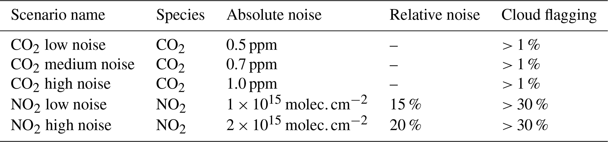
The synthetic observations were flagged as cloudy using the total cloud fractions simulated with the COSMO-GHG model. Since the CO2 retrieval requires strict cloud filtering, we removed all pixels with cloud fractions larger than 1 %. NO2 retrievals can tolerate higher cloud fractions. We used a cloud threshold of 30 % to flag cloudy pixels as often applied in satellite NO2 studies (e.g., Boersma et al., 2011).
3.1 Analytical inversion applied to the simulated plume
The analytical inversion uses the CO2 tracer representing the anthropogenic emissions of Berlin as simulated by the COSMO-GHG model. The method thus assumes perfect knowledge of atmospheric transport, which allows isolating the uncertainties in the flux inversion due to instrument noise. The inversion uses a forward model that computes the vector ymod of size m of model-simulated values at the locations of all XCO2 measurements within the plume. The plume was defined as those pixels for which the enhancement of the tracer is larger than a typical variability of the background field set to 0.05 ppm. The vector ymod is given by the equation
where x is a scalar representing the CO2 emission strength of Berlin. H is the observation operator representing the sensitivity of the XCO2 signal to changes in x, i.e., the emissions, in the satellite image. Since x is a scalar, H is a row matrix. It contains all XCO2 values obtained from the CO2 tracer simulated with constant emissions of Berlin that are larger than 0.05 ppm. yBG is the XCO2 background, which was computed from the model-simulated fields excluding the emissions from Berlin, consistent with the assumption of a perfect model with accurately known transport and anthropogenic and biospheric fluxes outside of Berlin.
The emission of Berlin was found as the maximum likelihood optimal estimate by minimizing the following cost function:
where yobs is the measurement vector containing the synthetic XCO2 observations. Sε is the error covariance matrix of the model–observation mismatch, which in our case of a perfect transport model corresponds to the measurement error covariance matrix. The diagonal elements of the error covariance matrix were set to the square of the absolute noise specified in Table 1.
The analytical inversion was applied to synthetic satellite observations with constant and time-varying emissions of Berlin. The uncertainty of the estimated emission was taken from the covariance matrix estimated by the least square fit. As a second measure of uncertainty, we computed mean bias (MB) and standard deviation (SD) of the differences between estimated and true emissions. Thereby, the true emission was taken at 10:30 UTC during satellite overpass. The plume may also contain emissions emitted earlier in the day, but the observation operator does not include information about the temporal variability of emissions. The variation in the diurnal cycle of emissions is rather small in the hours prior to the satellite overpass (Fig. S1 in the Supplement). Relative errors were computed relative to the annual mean at overpass time, which is 16.9 Mt CO2 yr−1 for constant and 20.0 Mt CO2 yr−1 for time-varying emissions. The latter is higher because emissions at 10:30 UTC are larger than daily mean emissions.
3.2 Mass-balance approach applied to the detected plume
The mass-balance approach estimates CO2 emissions from a city plume detected by a plume detection algorithm. The approach calculates CO2 mass fluxes from plume signals that are obtained by subtracting a background field from the satellite observations. The plume signal is then integrated perpendicular to the direction of propagation of the city plume to obtain line densities that are multiplied with an estimate of the wind speed to obtain the fluxes. Under the assumption of steady-state conditions, these fluxes are equivalent to the emissions.
The plume detection algorithm described in Kuhlmann et al. (2019a) was applied to determine the position of the CO2 plume in the satellite observations. The algorithm was applied either to the XCO2 observations or to the auxiliary NO2 observations. As shown in Kuhlmann et al. (2019a), the NO2 plumes largely overlap with the XCO2 plumes despite the fact that NOx is released in the model primarily at the surface by traffic emissions, whereas a larger proportion of CO2 is released from stacks at higher altitudes. The number and size of the detected plumes was significantly larger when the algorithm was applied to the NO2 measurements due to their better signal-to-noise ratio and lower sensitivity to clouds.
To obtain the plume signal, the background needs to be subtracted from the satellite observations. The CO2 background was estimated from the pixels surrounding the plume assuming that it is spatially smooth. To compute the background, all pixels within the detected plume were masked and replaced by interpolated values obtained by normalized convolution applied to the unmasked pixels surrounding the plume. The normalized convolution was performed with a Gaussian filter with σ = 10 pixels, i.e., a width of the Gaussian kernel of about 20 km.
Figure 1a shows a sketch of an CO2 city plume. To compute line densities, we draw 10 km wide boxes (nearly rectangular polygons) perpendicular to the plume's centerline. Line densities were computed for each box. Figure 1b shows the CO2 signals (in kg m−2) for one of the boxes. Choosing a box rather than a single line across the plume reduces the impact of noise and data gaps due to the larger number of available pixels. The across-plume width of the polygons is given by the maximum width of the detected plume plus an additional boundary of at least 10 km on each side to ensure that the entire plume is within the polygon even if only a part of the plume was detected.

Figure 1(a) Sketch of a CO2 city plume with detected pixels and fitted centerline. Random noise has been added to the CO2 observations. The center of the city source is denoted by S. The origin of the center curve is . For a satellite pixel P, the across-plume coordinate yp is the distance between P and Q, and the along-plume coordinate xp is the arc length from S to Q. The yellow rectangles are the polygons used for computing the line densities. (b) Example of CO2 mass columns in across-plume distance for the polygon containing the pixel P. (c) Line densities computed for each polygon in the sketch. The line densities are zero upstream of the source, build up over the city and remain constant downstream of the city.
The centerline of the plume was computed by fitting a two-dimensional curve to pixels within an extended plume area, which consisted of the detected plume as well as pixels within 50 km distance of the plume or the source. The surrounding pixels help stabilize the fit at the beginning and at the end of the detected plume. For the curve fit, pixels were weighted with the local mean values above background calculated by the plume detection algorithm. Outside the detected plumes, pixels were weighted either with a small value of 0.05 ppm or 0.2×10¹⁵ depending on whether CO2 or NO2 was used for plume detection. The two-dimensional curve p(r) consists of two parabolic polynomials:
with coefficients ak and bk and radial distance r. The parameter r is calculated as the distance from the origin:
where x and y are easting and northing in the DHDN/Soldner Berlin spatial reference system (EPSG: 3068). The origin (xo, yo) is placed at least 50 km away from the source in the direction opposite to the plume, i.e., in the west of Berlin if the plume is in the east and vice versa. Figure 1a shows the centerline with its origin O and the location of the source S.
To draw the polygons, pixel coordinates need to be converted to along- and across-plume coordinates for each satellite pixel. The across-plume coordinate yp is the distance between pixel P and the curve at radial distance rp, i.e., point Q in Fig. 1, for which the line from Q to P is perpendicular to the curve. The along-plume coordinate xp is the arc length of the center curve from the source origin S to Q. xp and yp were calculated with a computationally efficient analytical solution as presented in the Supplement.
To compute line densities from the CO2 columns inside the polygons (e.g., Fig. 1b), we tested two options: (1) integrating in across-plume direction yp by adding up the plume signals cp of all pixels whose center point is within the polygon and (2) fitting a Gaussian function to the plume signals in across-plume direction and computing its integral. The first method does not make any assumption about the shape of the cross section, which is an advantage for city plumes that can be quite complex. The disadvantage is that it is more difficult to deal with missing pixels, which lead to an underestimation of line densities if not properly accounted for. To solve this issue, we sub-divided the polygons in across-plume direction in 5 km wide sub-polygons, for which we computed a mean value from the available pixels. Finally, we integrated over the mean values of the sub-polygons. Polygons were not used if the mean values of at least one of the sub-polygons with detected plume pixels could not be computed due to missing values. Note that this criterion rejects more line densities from plumes detected from the NO2 observations than from the CO2 observations, because the latter detect narrower plumes.
The second method has been used, for example, by Reuter et al. (2019). Fitting a Gaussian curve has the advantage that it automatically interpolates missing values. The disadvantage is that the transects of a city plume do not necessarily resemble a Gaussian curve. The Gaussian curve can be written as
with line density q, shift μ and SD σ. To avoid misfits, especially when pixels near the center of the plume are missing, a Gaussian curve was only fitted if at least one valid observation was available in each sub-polygon in the transect. When NO2 observations are available, it is also possible to simultaneously fit a Gaussian curve to the NO2 observations using the same SD σ for both the CO2 and NO2 curve. Since the NO2 observations have a higher signal-to-noise ratio, the width of the CO2 curve is constrained by the NO2 observations. This method was demonstrated by Reuter et al. (2019) and is used here as a third method.
An estimate of the mean flow speed within each plume transect is required to convert line densities to emissions. The mean flow speed is the projection of the CO2-weighted wind vector onto the along-plume direction. Because we assume not to know the vertical and horizontal distribution of winds and CO2 concentrations sufficiently well from a model, we take the average wind speed at the location of Berlin in the lowest 500 m above surface assuming a well-mixed boundary layer as a rough estimate. The wind profile was taken from the COSMO-GHG model simulations at satellite overpass time but could be taken from any meteorological analysis data. Not taking the wind speeds directly at the locations of the cross sections was an attempt to account for uncertainties in the simulated winds that would be encountered with real rather than synthetic observations. To estimate the uncertainty in this simplified estimate of the mean flow speed, we also computed an effective wind speed for each polygon, taking into account the three-dimensional distribution of winds and CO2 mass concentrations. The effective wind speed is the weighted mean wind speed parallel to the plume's centerline and weighted by the partial CO2 mass column density of the plume. These CO2 column densities are taken from the model tracer that contains only emissions of the city.
Figure 1c shows line densities computed in along-plume direction. The line densities are zero upstream of the source, build up over the city and remain constant downstream of the city. The fluxes were obtained by multiplying the line densities with the wind speed. Finally, the fluxes were averaged to obtain an estimate of the mean source strength. We only considered values more than 10 km downstream of the city center to ensure that fluxes are obtained from outside of the city area. Uncertainties in the mean source strength were computed from the standard error of the individual line densities as well as by comparing with the true emissions at overpass.
To better understand the individual error components, the differences between estimated and true emissions were further analyzed using the detailed information available from the simulation. For this purpose, the mass-balance approach was additionally applied to the detected plume using the noise-free XCO2 observations, the true CO2 background and the effective wind speed. By replacing the uncertain information obtained from the observations with the accurate information from the model, four different types of error were distinguished.
-
The method error is the difference between the true emissions at satellite overpass and the emissions computed using the model information. It represents the intrinsic uncertainties of the method that arise from simplified assumptions such as constant emissions and wind speed, from the plume detection algorithm, and from the fitting of the centerline.
-
The retrieval error represents the impact of the random noise in the CO2 observations on the calculation of line densities.
-
The background error is caused by errors in the estimation of the background field and its impact on the computed plume signals.
-
The wind error is the error that occurs if the mean wind speed between 0 and 500 m above Berlin is taken instead of the effective mean wind speed within the plume.
Note that these different error types are still strongly related to the size of detected plume and thus, in the case of the CO2-based plume detection, to the instrument noise scenario. These errors were therefore calculated separately for the different noise scenarios.
3.3 Estimating annual emissions
To estimate annual emissions and their uncertainties, the temporal variability of emission has to be considered, which includes seasonal, diurnal and weekend vs. weekday variations. Without accounting for this variability, annual mean estimates derived from a small sample of satellite overpasses at a fixed time of the day may be significantly biased.
In this study, only the seasonal cycle was estimated using a Hermite spline with periodic boundary conditions (see Supplement). The periodic boundary conditions help constrain the cycle in winter months, where only few data points are available. To properly fit the seasonal cycle, we used a spline with four equidistant knots. The annual emissions were then estimated by integrating over the seasonal cycle. The uncertainty of the annual emissions was estimated by error propagation from the precision of the CO2 emission estimates at individual satellite overpasses. Since annual emissions estimated in this way are only representative of emissions a few hours before the satellite overpass, the estimated emissions were compared with the emissions at overpass time. Uncertainties in the ratio between emissions at overpass time and daily mean emissions are thus not taken into account.
4.1 CO2 emissions estimated by analytical inversion
The analytical inversion was applied to all CO2 plumes observed by the CO2 satellites for constant and time-varying emissions and for the low-, medium- and high-noise scenarios with σVEG50 of 0.5, 0.7 and 1.0 ppm, respectively. Figure 2a and c show the time series of estimated CO2 emissions for the medium-noise scenario (σVEG50=0.7 ppm) with a constellation of three satellites. CO2 estimates with uncertainties larger than 10 Mt yr−1, i.e., 50 % of the mean emissions at satellite overpass time for time-varying emissions, were discarded to remove plumes with very weak CO2 signals or with a small number of pixels.
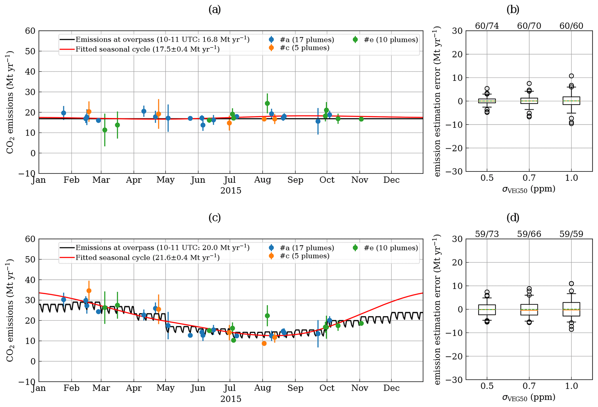
Figure 2Time series of CO2 emissions of Berlin estimated with the analytical inversion using three satellites (#a, #c and #e) with σVEG50 of 0.7 ppm for (a) constant and (c) time-varying emissions. Emission estimates with uncertainties larger than 10.0 Mt yr−1 (50 % of mean emissions at 11:30 LT) were removed. (b, d) Boxplots of the difference between estimated and true CO2 emissions of Berlin using six satellites for the three different instrument noise scenarios. The boxes denote the range between 25th and 75th percentiles, orange lines are median values, dashed lines are mean values, and whiskers are 5th and 95th percentiles. The numbers above the boxes are the cases where the uncertainties for all three scenarios are less than 50 % (first number) and the number of successful emission estimates for each scenario (second number).
The boxplots (Fig. 2b and d) summarize the differences between estimated and true emissions for all plumes observed by the six satellites. A constellation of six satellites was able to estimate emissions successfully, i.e., with an uncertainty smaller than 10 Mt yr−1, for 60 to 74 overpasses for time-constant emissions and 59 to 73 overpasses for time-varying emissions depending on the noise scenario. The average number of successful estimates was 11 per satellite and year but with a large range from 5 to 17 because of varying cloud coverage and because some orbits cover Berlin less frequently than others. Table 2 shows mean bias (MB) and standard deviation (SD) of the differences between estimated and true emissions. To compute comparable statistics for each instrument scenario, the statistics were computed only for the 60 and 59 plumes, respectively, for which the uncertainties were less than 10 Mt yr−1 in all three noise scenarios.
Table 2Performance of the analytical inversion for individual satellite overpasses in terms of mean bias (MB) and standard deviation (SD) of the difference between estimated and true CO2 emissions of Berlin. More plumes could have been used for emission quantification for scenarios with low noise (second value in column “Number of plumes”), but the statistics were computed only for those plumes that could be used with the high-noise scenario (first value) for better comparability of the results.

The constant emissions are generally well captured within the uncertainty range determined by the measurement noise. The uncertainties of the individual estimates vary strongly because the amplitudes and sizes of the plumes differ from case to case due to differences in wind speeds, cloud cover and incomplete coverage of the plume by the swath. The MB is close to zero for all noise scenarios.
In the case of time-varying emissions, the seasonal cycle of the emissions can be reproduced quite accurately because many plumes can be observed with three or more satellites and because the individual estimates have an average uncertainty of only 14 %–21 % depending on instrument noise scenario. The rare opportunities for observing plumes in winter due to frequent cloud cover, however, can easily be missed by a small constellation of satellites, which will make it difficult to reliably trace the seasonal cycle. The MB slightly deviates from zero (Table 2) mainly because the observation operator H was calculated assuming constant emissions, while the measurement vector contains observations of time-varying emissions from several hours before the satellite overpass time. The SDs of the differences between the individual emission estimates and the true emissions are 3.0, 3.4 and 4.2 Mt yr−1 for σVEG50 of 0.5, 0.7 and 1.0 ppm, respectively (Table 2). These values agree well with the mean of the estimated uncertainties, suggesting that the error propagation yields a realistic estimate of uncertainties.
The theoretical uncertainty computed by the inversion agrees well with the SDs computed for constant and time-varying emissions in Table 2. This estimated uncertainty depends on the number of pixels and the signal strength of the plume. The signal strength in turn depends on the wind speed and turbulent mixing. Figure 3 shows the dependency of the theoretical uncertainty on the inverse of the square root of the number of pixels and on wind speed for the medium-noise scenario. Fitting a robust linear regression model yielded
with number of pixels n and wind speed u. The uncertainty depends strongly on the number of pixels and is smaller than 10 Mt yr−1 (50 %) if the number of pixels is larger than 100 for all three noise scenarios. The dependency on wind speed is less robust and does not depend on the noise scenario. Most outliers are due to plumes of less than 100 pixels. Note that the fit coefficients are specific to the emissions and meteorological conditions of Berlin and cannot be generalized for other cities.
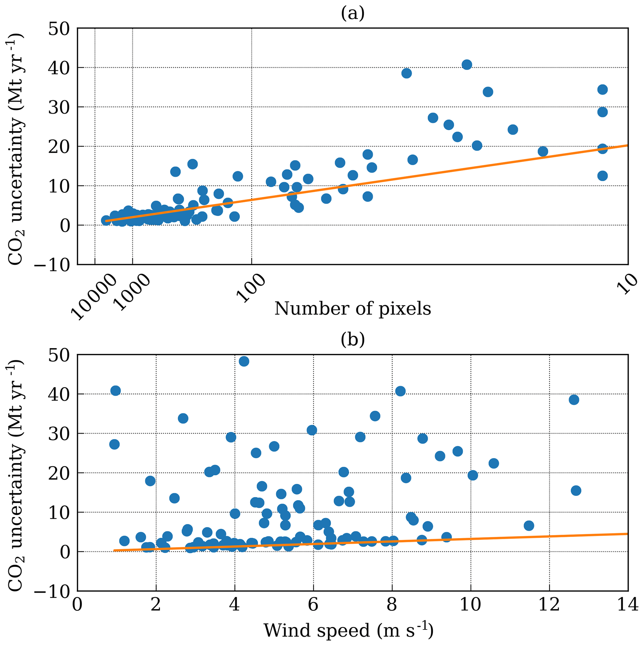
Figure 3Dependency of the theoretical CO2 uncertainty on (a) inverse of the square root of the number of pixels and (b) wind speed. The line is the fit of a multilinear regression model that was used to determine the slope of the linear dependence on these quantities.
4.2 CO2 emissions estimated by mass-balance approach
The mass-balance approach was applied to synthetic observations of the CO2M mission for a constellation of up to six satellites using the uncertainty scenarios with σVEG50 of 0.5, 0.7 and 1.0 ppm. The location of the CO2 plumes was either detected from the CO2 observations alone or from the additional NO2 observations on board the same satellite.
4.2.1 Example for 23 April 2015
The method is illustrated in Figs. 4 and 5 for a plume on 23 April 2015. In Fig. 4a, the CO2 plume is hardly visible, because its signal-to-noise ratio is close to 1. In contrast, the NO2 plume is clearly visible in the NO2 image (Fig. 5a). The plume detected from the CO2 observations (Fig. 4) is significantly smaller than the plume detected from the NO2 observations (Fig. 5) (119 vs. 780 pixels). The plume detected from the CO2 observations is also shorter with a length of 60 km as opposed to 120 km. This results in having fewer polygons for computing line densities. Finally, the plume detected from the CO2 observations is also narrower, suggesting that a significant part of the real plume is attributed to the background.
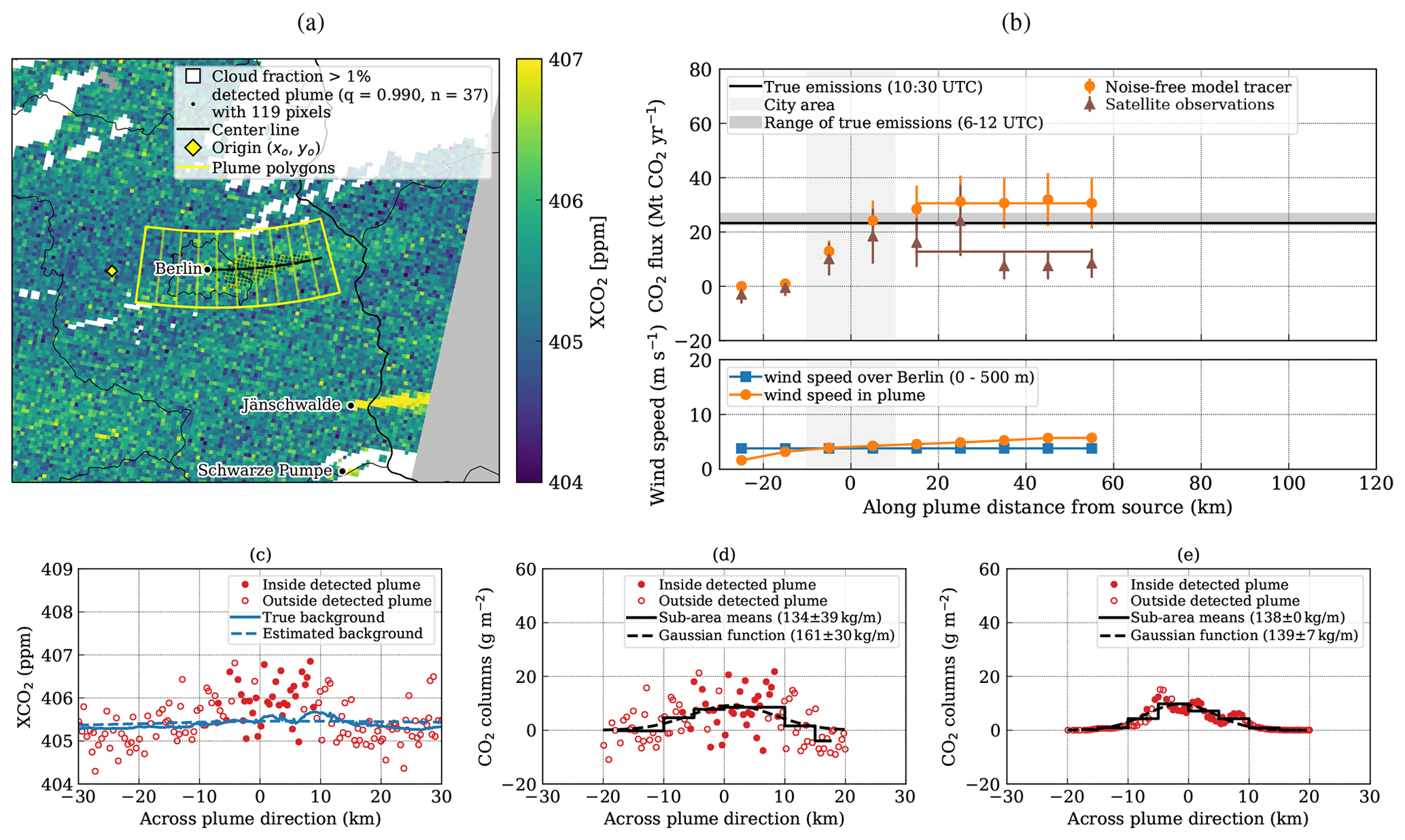
Figure 4Illustration of the mass-balance approach applied to a plume on 23 April 2015 observed with low-noise CO2 observations. (a) Detected XCO2 plume with polygons used for computing the line densities. (b) CO2 flux and wind speed as a function of along-plume distance. The CO2 fluxes estimated from the line densities are shown as markers with their uncertainty for the noise-free model tracer and the synthetic satellite observations. The horizontal lines show true emissions of Berlin at 10:30 UTC (black line) and the estimated emissions. The extent of the city is highlighted by the light gray area. (c) XCO2 satellite observations as a function of across-plume distance in the polygon between 10 and 20 km downstream of the source. (d) Same as panel (c) but CO2 column densities after subtracting the estimated background field. Sub-polygon means and Gaussian fit are also shown. (e) CO2 column densities from the model tracer containing only emissions of Berlin.
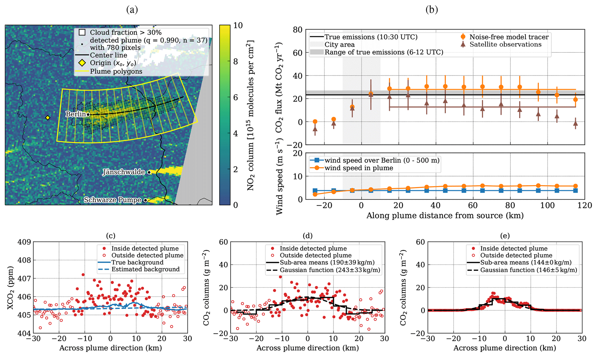
Figure 5Same as Fig. 4 but using the NO2 observations for detecting the plume.
The CO2 concentrations were plotted in across-plume direction for the polygon between 10 and 20 km downstream of the center of Berlin (Figs. 4c–e and 5c–e) The XCO2 signal in the plume is only about 1 ppm above background, which is comparable to the instrument noise of 0.5 to 1.0 ppm of the three instrument scenarios. A 1 ppm enhancement approximately corresponds to a CO2 column density of 10 g m−2. The model tracer representing the emissions of Berlin shows three distinct enhancements rather than a single Gaussian-shaped plume caused by the three power stations in Berlin (Fig. 4e). Nonetheless, the line density obtained by fitting the values from the model tracer with a Gaussian curve agrees well with the line density computed from the mean values in the sub-polygons. Note that the line densities were only computed between −20 and 20 km from the centerline, because pixels more than 10 km outside the detected plume were masked to avoid issues from neighboring plumes or variability in the CO2 background. Since the plume detected from the NO2 observations is wider, the line densities from the model tracer are slightly higher, because the plume edges still contain some CO2 emitted from Berlin (Fig. 5e).
Figure 4d shows the across-plume column densities from the satellite observations after subtracting the estimated background. The line densities are 134±25 and 161±30 kg m−1 using the mean values in the sub-polygons and the Gaussian fit, respectively. The uncertainty was computed from the random noise of the measurements for the sub-polygon means and from the quality of the fit for the Gaussian function. Figure 5d shows the same for the plume detected from the NO2 observations. In this case, the line densities are higher with 190±40 and 243±33 kg m−1. The reason for these differences is on the one hand the larger and slightly shifted polygon due to the different plume detection and on the other hand because the estimated CO2 background is different when CO2 or NO2 observations are used for plume detection (see Sect. 4.3 for details).
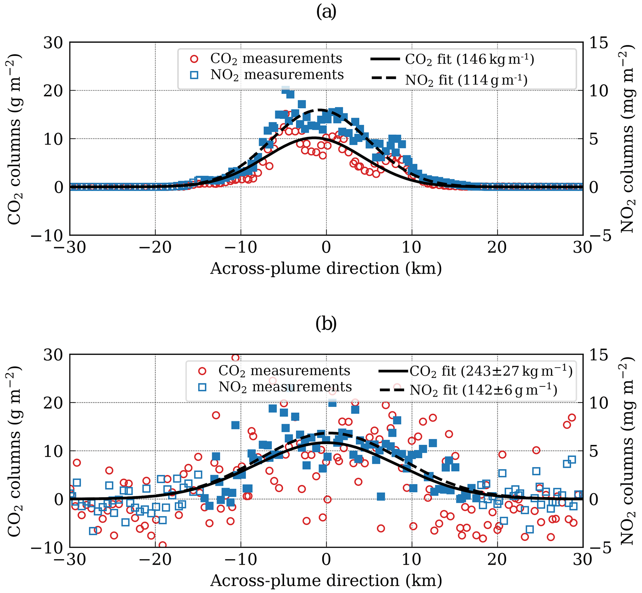
Figure 6Line densities computed from (a) the model tracer and (b) synthetic satellite observations using the Gaussian curve constrained by the NO2 observations.
The line densities in along-plume direction are shown in Figs. 4b and 5b. Upstream of the city, the line densities are close to zero and then slowly build up over the city. They reach their maximum downstream of the city and stay constant because CO2 does not decay in the atmosphere. The figures also show the mean and effective wind speed along the plume. While the average wind speed is constant, the effective wind speed is lower near the city center where the CO2 plume is still near the surface where wind speeds are lower. The mean height of the plume increases downstream of the city, and, therefore, the effective wind speed also generally increases with distance from the city. The CO2 fluxes computed from the noise-free model tracer are higher than the true emissions in this example, which is caused by the simplifications in the mass-balance approach, mainly by the assumption of a constant flow parallel to the fitted center curve. The fluxes computed from the synthetic satellite observations are lower than the true emissions at overpass. Near the source, the error is quite small, but it gets larger downstream mainly due to growing systematic errors in the estimation of the background, since it gets increasingly difficult to separate the plume from the background in the fading plume.
Figure 6 shows the same CO2 across-plume column densities from the model tracer and the satellite observations as Fig. 5, but it shows additionally the NO2 column densities. The CO2 line density was obtained by fitting a Gaussian curve whose width was constrained by the additional NO2 observations. While the line density is the same as without constraining the width of the curve for the present example, the estimated uncertainty is smaller.
4.2.2 Time series of estimated emissions
With six satellites, the NO2-based plume detection could identify about 40 plumes suitable for applying the mass-balance approach. On average, seven plumes were identified per satellite, but with a very large spread between the satellites (range: 1–14) because some orbits are more suitable than others for observing Berlin as mentioned earlier. In addition, since the number of overpasses is small, the uneven distribution of cloud-free days in time can have a large effect on the number of plume observations for a given satellite. From the CO2 observations alone only about half of these plumes could be detected because of the lower signal-to-noise ratio and the more stringent cloud filtering required for the CO2 observations.
Because of the different cloud thresholds for CO2 and NO2, some of the plumes detected from the NO2 observations do not have enough cloud-free CO2 pixels for computing line densities and can therefore not be used for estimating emissions. The NO2-based plume detection generally results in significantly more pixels per plume with about 400 to 800 pixels compared to less than 300 pixels for CO2-based detection. More details about the detectability of CO2 plumes from the CO2 and NO2 observations are presented in Kuhlmann et al. (2019a).
Before applying the mass-balance approach, the detected plumes and the centerlines were visually inspected to remove plumes with obvious issues. In particular, for the CO2-based plume detection several plumes were removed for which the number of detected pixels was too small to reliably fit a centerline parallel to the wind direction. In most cases, 50 or more detected pixels were sufficient. Often less than 100 pixels were detected from the high-noise CO2 observations, but it was often still possible to use these plumes with less than 100 pixels for estimating emissions. Three plumes were removed where the CO2 plume of the Jänschwalde power plant overlapped with the plume of Berlin. In many cases, the CO2 image alone did not show clearly which plumes had a reasonable centerline, and therefore additional information such as wind fields is helpful. The NO2 images are also extremely helpful, because they are less affected by clouds and often reveal weak interfering plumes in the surrounding area that are not detectable from the CO2 observations.
The number of plumes remaining for reliable emission estimation was 34 for plumes detected from the NO2 observations, which are only between 0 and 10 plumes per satellite and year with an average number of 5.7. These numbers would be approximately halved with the CO2 observations alone: 16 to 17 plumes could be used with six satellites for the different noise scenarios, i.e., on average only 2.7 (range: 1–7) per satellite.
Figure 7a and c present the time series of estimated CO2 emissions for these plumes. The time series is shown for a constellation of three satellites for the medium-noise scenario (σVEG50±0.7 ppm) and line densities computed from the sub-polygon means. The time series for a less likely constellation of six satellites are shown in the supplement. The error bars show constant errors of 10.0 Mt yr−1 corresponding to the SD of the differences between estimated and real emissions.
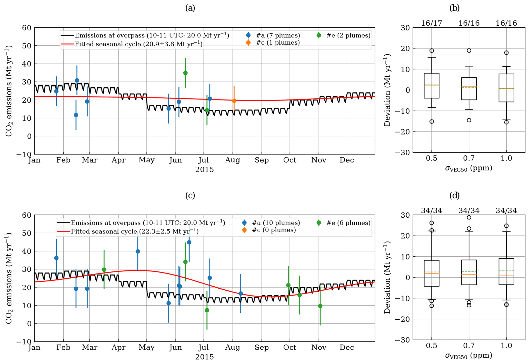
Figure 7Time series of estimated CO2 emissions of Berlin using a constellation of three satellites (#a, #c and #e) with medium-noise instruments (σVEG50=0.7 ppm). The plumes were detected from (a) the CO2 and (c) the NO2 observations. The error bars show constant errors of 10.0 Mt yr−1 corresponding to the SD of the differences between estimated and real emissions. (b, d) The boxplots show the difference between estimated and CO2 emissions at overpass of Berlin for six satellites. The boxes denote the range between 25th and 75th percentiles, orange lines are median values, and whiskers are 5th and 95th percentiles. The numbers above the boxes are the number of cases for which emissions could be estimated for all three scenarios (first number) and the number of successful emission estimates for each scenario (second number).
A constellation of three CO2M satellites without additional NO2 observations can detect plumes and estimate emissions from only 10 overpasses. These overpasses are likely to cluster in specific months with good weather conditions leaving significant gaps in other months. A constellation of six satellites is able to detect more plumes proving better temporal coverage of the different seasons. This can also be achieved when NO2 observations are available for plume detection. In this case, 16 plumes can already be used with a constellation of three satellites.
Note that for a few overpasses where the emissions were estimated from the plume detected from the CO2 observations (e.g., the only estimate from satellite #c), the emissions were not estimated from the plume detected from the NO2 observations. In these cases, only a fraction of the full plume was detected from the CO2 observations, because the plume was partly covered by clouds, while a larger plume could be detected from the NO2 observations. Since our algorithm rejects line densities with missing observations in sub-polygons, no emissions were calculated for cases where this affected all line densities.
4.3 Uncertainties in the mass-balance approach
As expected, uncertainties in the estimated emissions are larger for the mass-balance approach compared to the analytical inversion. Figure 7b and d show the difference between estimated emissions and the emissions at overpass for different noise levels of the CO2 instrument. These boxplots include all estimates for a constellation of six satellites.
Table 3 shows MB and SD of these differences. For better comparability, these statistics were computed only from those plumes that could be detected with all three noise scenarios, i.e., 16 plumes in the case of CO2-based detection and 34 plumes in the case of NO2-based detection. SDs are about 10 Mt yr−1, i.e., about 50 % of the 20.0 Mt yr−1 emissions of Berlin at overpass time, which is about 3 times larger than for the analytical inversion. For the plume detection based on the CO2 observations, SDs are about 9 Mt yr−1 (45 %) and, interestingly, do not depend significantly on the noise level of the instrument. SDs are slightly larger with 10 Mt yr−1 (50 %) if the NO2 observations are used for plume detection, because applying the mass-balance approach to larger plumes is more challenging.
Table 3Mean bias (MB) and standard deviation (SD) of differences between estimated CO2 emissions and emissions at overpass time (10:00–11:00 UTC) for Berlin based on observations with six satellites. The CO2 plume was either detected from CO2 or NO2 observations (high-noise scenario). The results are for line densities computed from the sub-polygon means.

The MB is positive for both CO2- and NO2-based plume detection. With NO2-based plume detection it rises slightly from 2.6 to 3.5 Mt yr−1 (13 %–17 %) from the low to the high-noise scenario. With CO2-based detection, in contrast, the lowest MB is surprisingly obtained for the high-noise scenario.
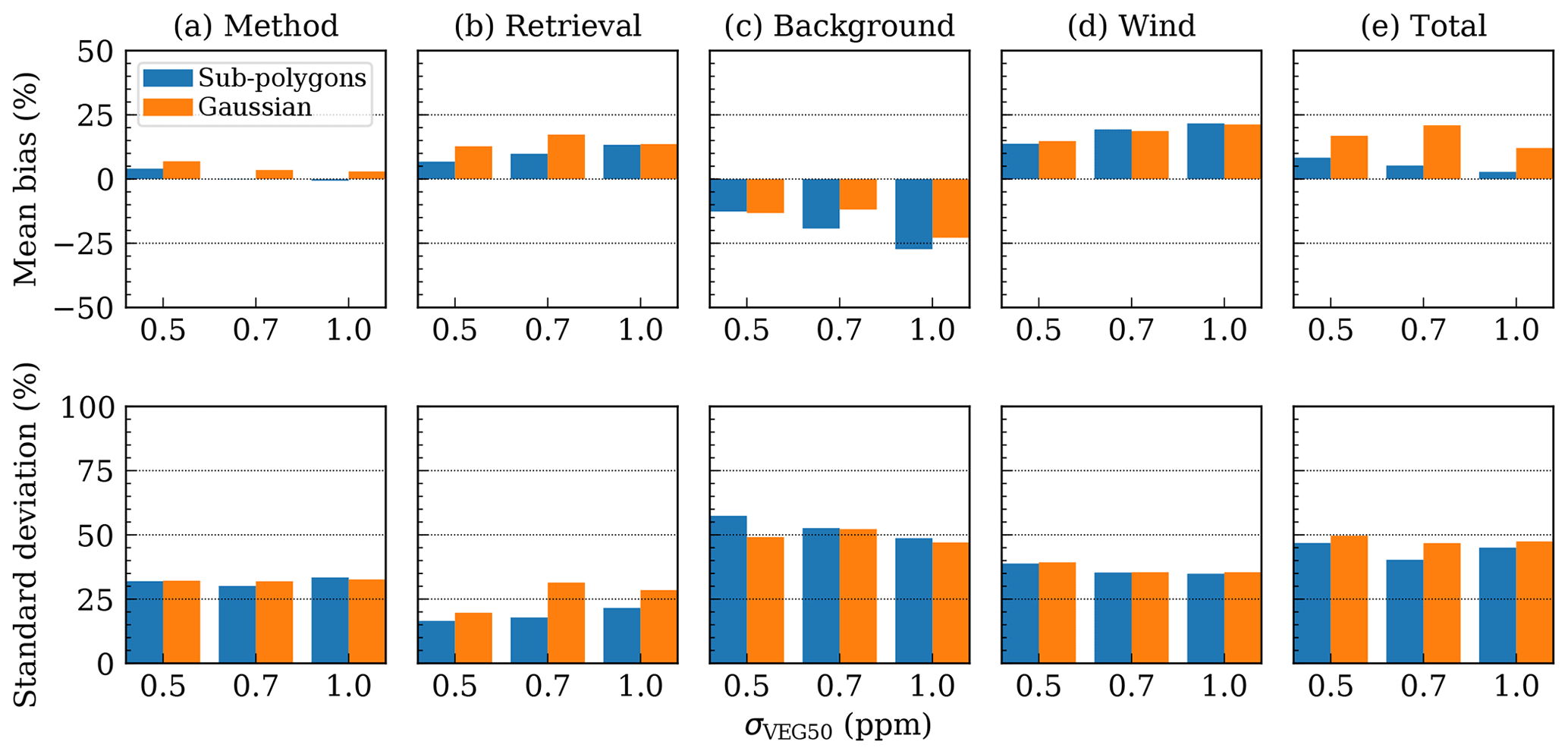
Figure 8Mean bias (MB) and standard deviation (SD) of (a) method, (b) retrieval, (c) background, (d) wind and (e) total errors for CO2-based plume detection. MB and SD are shown for the three uncertainty scenarios and for line densities computed from sub-polygon means and Gaussian function, respectively.
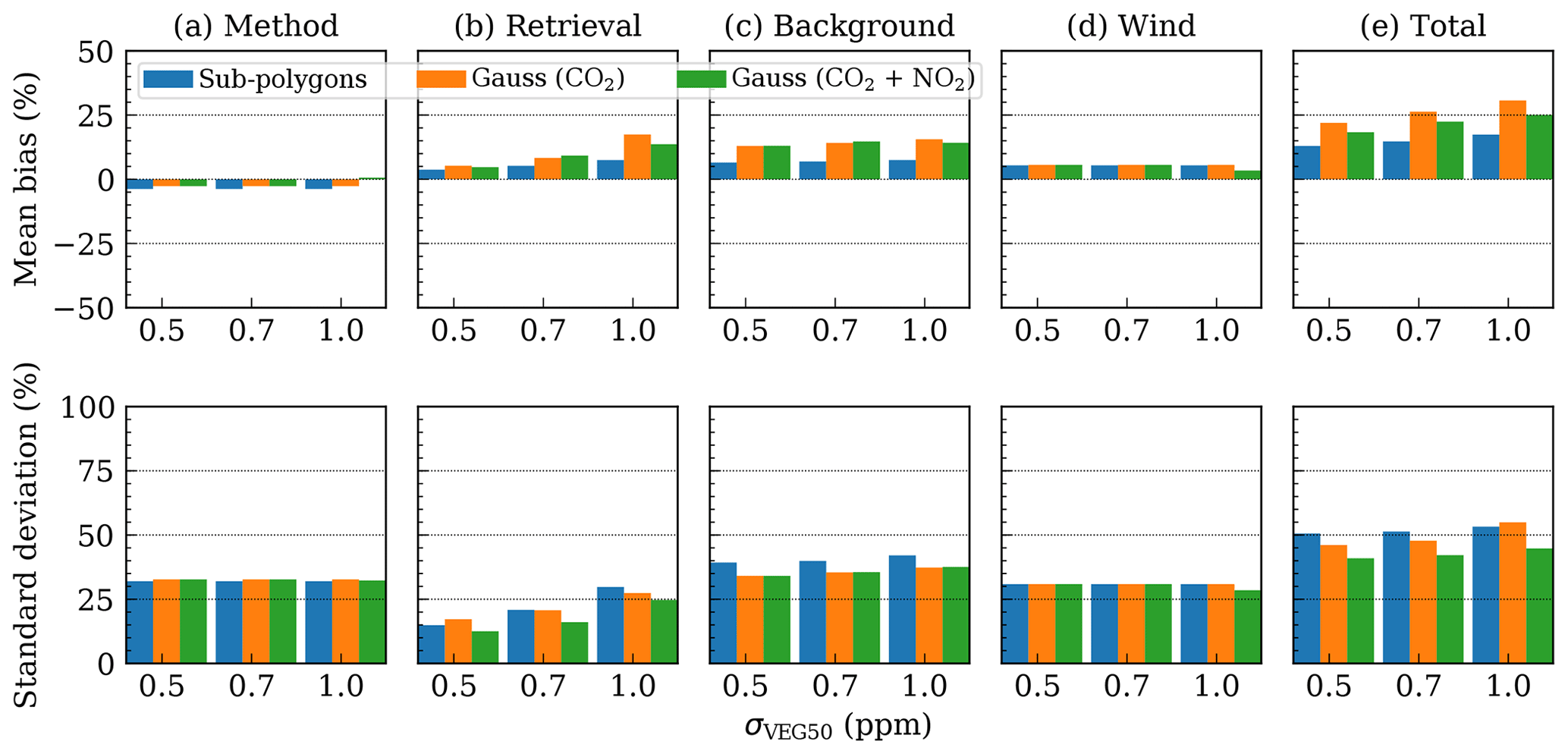
The MB is caused by systematic errors in the method, retrieval, background and wind errors, which can have substantial systematic errors that may add up or compensate for each other in the total error. The results therefore need to be interpreted with great care. MB and SD of the individual error components are summarized for the different noise scenarios in Figs. 8 and 9 for CO2 and NO2-based plume detection, respectively. The method and total errors are computed against the true emissions at overpass, while the other errors are compared to the emissions computed using the model information. The total errors are identical to the errors presented in Table 3. The relative MB and SD are tabulated in the supplement. The different errors are discussed in detail in the following.
4.3.1 Method error
The mass-balance approach relies on assumptions and simplifications that result in uncertainties in the estimated emissions. The main sources of uncertainty are the assumption of constant emissions and constant flow parallel to the centerline fitted to the detected plume. The method error also indirectly depends on the instrument noise scenario that affects the size of the detected plumes.
Figures 8a and 9a show that the MB is slightly positive when plumes were detected from CO2 observations and slightly negative when plumes were detected from NO2 observations. The absolute MB is mostly smaller than 5 %, suggesting that the assumptions in the mass-balance approach do not cause significant systematic errors. In particular, we do not find that emissions are overestimated, although we compared estimated emissions with emissions at overpass (10:30 UTC), while the plume may also contain CO2 released a few hours earlier when emissions are higher (Fig. S1). Note that such a bias would also affect the analytical inversion.
The SD of the method error is about 30 %, which gives a rough estimate of the minimum SD achievable with the mass-balance approach. The SD does not depend on the instrument noise scenario or whether CO2 or NO2 was used to detect the plume despite the influence this has on the size of the detected plume.
4.3.2 Retrieval error
The retrieval error shown here is affected mainly by the computation of the line densities from the noisy CO2 observations, because the effect of the retrieval error on the plume detection algorithm is part of other error components. Figures 8b and 9b show that the SD of the retrieval error roughly doubles from the low-noise scenario to the high-noise scenario, which is consistent with the doubling of the random error in the instrument scenarios. The SD is similar to the uncertainty found in the analytical inversion (Table 2), which also only includes errors from the instrument noise.
The retrieval error has a small positive bias that scales with the absolute noise of the uncertainty scenarios. The reason that the MB scales with the absolute noise is that the same random errors, i.e., spatial noise pattern, were applied to the three uncertainty scenarios of a scene except for a scaling required to achieve the SD of the error σVEG50. Since no systematic errors were applied to the satellite observations, we would expect that the MB of the retrieval error is closer to zero. A likely explanation for the positive MB is that the plume detection algorithm is more likely to detect CO2 pixels that are positive outliers, i.e., CO2 values that have a large positive random error. If these outliers are included when computing line densities, they result in a positive bias in the estimated emissions. This artifact also affects plumes detected from NO2 observations, because the same noise pattern was applied to CO2 and NO2 observations. While this is partly an artifact from setting up the OSSE in order to allow for comparison between the different instrument scenarios, it might also appear in real observations.
If line densities are calculated by fitting a Gaussian function to the plume detected from the CO2 observations, SDs are higher likely due to the challenge of fitting the curve through data with a low signal-to-noise ratio and because the detected plume is narrow and does not include many background values outside the plume that would help stabilize the baseline (Fig. 4d). Furthermore, the transect of the city plume often does not resemble a Gaussian curve, which results in an additional fitting error. In contrast, SDs are reduced when the curve is fitted by constraining its width using the NO2 observations resulting in the lowest SDs of the retrieval errors.
4.3.3 Background error
The CO2 background has a strong impact on the estimated emissions, because a bias in the background field results in a bias in the CO2 signals and thus in the estimated emissions. Figure 10 presents two examples of estimated and true CO2 backgrounds for 27 February and 23 April 2015, respectively. The true CO2 background was taken from the model tracer that includes all emissions and fluxes except emissions from Berlin. The background fields in the mass-balance approach were estimated using the plume detected from the NO2 observations (black dots). On 27 February, the CO2 background field has a strong horizontal gradient and the wind speed is relative low with 2 m s−1. On 23 April, the background has no gradient and the wind speed is somewhat higher with 6 m s−1. In general, the estimated background field is smoother than the true background field, which displays fine-scale patterns associated with meteorology and CO2 fluxes. The MB of the differences within the detected plume is −0.03 ppm on 27 February and +0.04 ppm on 23 April, which is small compared to the amplitude of Berlin's plume signal of about 1 ppm. The SD is 0.11 ppm within the detected plume for both overpasses, which is much smaller than the noise of the CO2 observations (σVEG50: 0.5 to 1.0 ppm).
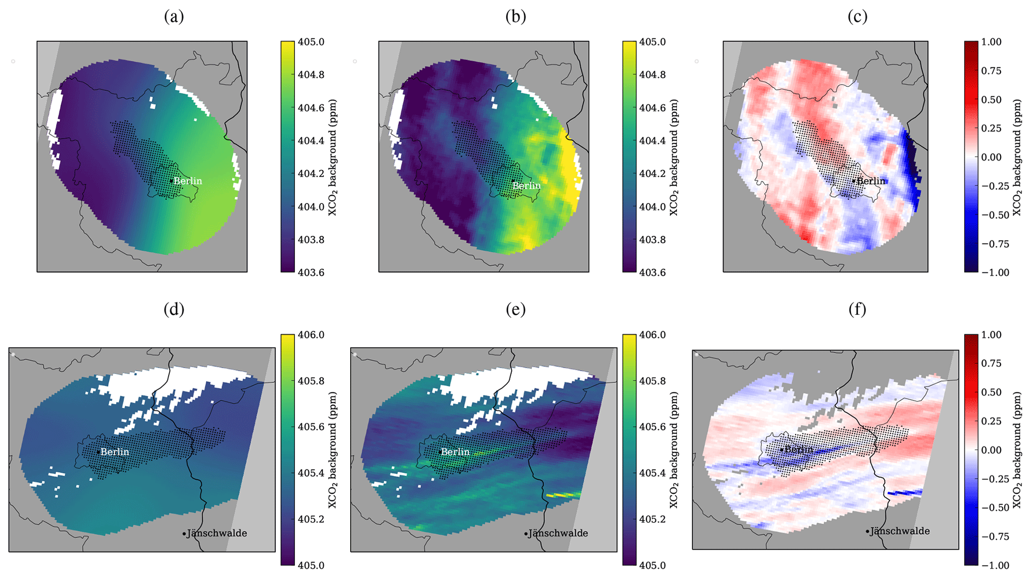
Figure 10(a) Estimated background, (b) true background, and (c) difference between estimated and true background for 27 February 2015. Black dots show the CO2 plume detected from the NO2 observations. Mean bias (MB) and standard deviation (SD) within the detected plume are −0.03 and 0.11 ppm. (d–f) The same as (a–c) but for 23 April 2015 with MB and SD of 0.04 and 0.11 ppm, respectively. Note that MB and SD are much smaller than the noise of the measurements. The effective wind speeds within the plumes are 2 and 6 m s−1, respectively.
However, the differences between estimated and true background vary spatially with local biases up to ± 0.3 ppm (see Fig. 10c and f). The size, shape and orientation of these patches depend on wind speed and direction. The patterns are caused by the effect of meteorology on CO2 from anthropogenic emissions outside of Berlin and biospheric fluxes inside and outside of Berlin. Since the size of the patches is similar to the size of the polygons used for computing the line densities, the local biases in the background can result in biases in the line densities. For example, a MB of 0.1 ppm within a polygon would overestimate the line density by about 30 kg m−1 for a typical plume width of 20 km. For Berlin, we expect line densities of about 110 to 320 kg m−1 for emissions of 20 Mt yr−1, if we use wind speeds of 6 and 2 m s−1, respectively. As a result, the comparative small bias of 0.1 ppm would result in a bias in the estimated emissions of 10 % and 30 %. Since the patterns are rather random, the resulting errors would mostly show up in the SD of the background error, and they would decrease if several line densities were computed per plume. As plumes detected from NO2 observations are larger, SDs are expected to be smaller. Indeed, this can be seen in the SDs of the background error, which are about 50 % vs. 40 % for CO2- and NO2-based plume detection, respectively (Figs. 8c and 9c).
The CO2 background concentrations obtained from the plumes detected from the CO2 observations are slightly higher (0.08 ppm on average) than the backgrounds from the plumes detected from the NO2 observations. The reason is that the plumes detected from the CO2 observations are smaller and thus pixels outside the plume have higher CO2 values, because they still contain some enhanced values from the Berlin plume or other smaller plumes in the vicinity. As a consequence, the size of the detected plume has an impact on the MB of the background error. For CO2-based plume detection, the emissions are underestimated by 10 % to 30 %. The effect increases with instrument noise, because detected plume size decreases.
On the other hand, the plume detected from the NO2 observations is larger and thus includes all emission of Berlin but might also include emissions in the vicinity of Berlin. Therefore, the mass-balance approach does not only estimate emissions from Berlin, but also emissions from sources outside. Since there are no large point sources just outside the city boundaries, emissions from outside of Berlin are relative small. The CO2 emissions from outside Berlin are 4.2 Mt yr−1 (20 % of Berlin's annual emissions at overpass) within a radius of 25 km around Berlin's city center. On average, emissions estimated from the plume detected from the NO2 observations are about 10 % higher than Berlin's emissions. It is therefore necessary to interpret the emissions determined with the mass-balance approach as emissions from a footprint that may be larger than the area of the city (e.g., Pitt et al., 2019).
4.3.4 Wind error
The wind error computed here includes only the difference between the mean wind below 500 m and the effective mean wind speed within the detected plume. For the NO2-based plume detection, its MB is close to zero (+0.04 m s−1, i.e., <1 %) with a SD of about 1.6 m s−1 (32 %) for the 34 cases with successful estimates. The mean effective wind speed for these cases is 5.2 m s−1, which has been used to compute the relative error. If CO2 observations are used for detecting the plume, the mean difference increases from 0.5 to 0.7 m s−1 (14 %–19 %) for the low- to high-noise scenario, and the SD is about 1.2 m s−1 (33 %) where the effective wind speed was 3.7 m s−1 for the 16 plumes.
The small MB with NO2-based plume detection shows that the mean wind between 0 and 500 m was a suitable estimate of the effective wind speed in the detected plume. The MB increases for the CO2-based plume detection, because mostly pixels in the vicinity of Berlin are detected from the CO2 observations, while the plumes detected from the NO2 observations extend further downstream. In the vicinity of the sources, the effective plume height is lower than further downstream, because the city plume has undergone less vertical mixing. Consequently, the effective wind speed is also smaller, because wind speed is lower near the surface. The small overestimation of the wind speed results in a significant overestimation of emissions of about 6 % and 14 % to 22 % for the NO2- and CO2-based plume detection, respectively. The SD of the wind error leads to an error in the estimated emissions of 30 % to 40 %.
We used the wind profile over the city of Berlin instead of the wind inside the plume to account for model errors in the estimated wind speed. As a result, SDs of the wind error were quite large (1–2 m s−1) but likely realistic, because they are of a similar magnitude as difference between measured and simulated winds in model validation studies (e.g., Sharp et al., 2015). Although the mean wind between 0 and 500 m was found to be a suitable estimate of the effective wind speed in this study, the choice of altitude range was rather arbitrary. Averaging the wind, for example, between 0 and 1 km would overestimate emissions by 15 % on average as the wind speeds are higher. Choosing an optimal altitude range is thus one of the largest challenges of the mass-balance approach.
4.3.5 Total error
The breakdown of the errors shows that method, background and wind error strongly contribute to the total error, while the influence of the retrieval error is comparatively small. Since the MB of the background error is negative for plumes detected from the CO2 observations, the positive retrieval and wind errors are partially compensated for, resulting in the decrease in the MB with increasing instrument noise (Table 3).
Our study did not include systematic errors from aerosols, clouds and surface reflectance in the satellite observations. Such systematic errors can lead to large-scale biases, which would not affect the results if they influenced the observations inside and outside the city plume in the same way. However, systematic error patterns correlated with the CO2 plumes, caused for example by enhanced aerosol concentrations in the city plume, could lead to biased emission estimates. Such effects are currently investigated in a study on the use of aerosol information for estimating fossil fuel CO2 emissions (AEROCARB). They showed that the proposed CO2M aerosol instrument (i.e., a multi-angle polarimeter) can reduce systematic errors due to aerosols to a level suitable for monitoring CO2 emissions from cities (Houweling et al., 2019).
The NOx chemistry used in our simulations was highly simplified, accounting only for a constant NOx lifetime of 4 h. Laughner and Cohen (2019) recently estimated NOx lifetimes of North American cities from satellite observation and found annual mean lifetimes varying between 1 and 5 h for different cities. In our study, a shorter lifetime would result in NO2 signals that decrease faster downstream, and therefore the detectable plume would be correspondingly shorter. A different plume length will reduce the number of polygons available for computing line densities and thus could impact the SD of the retrieval error. Berlin's mean plume length was about 90 km for plumes detected from the NO2 observations. A lifetime of 2 h would reduce the plume length to about 45 km, which is the mean plume length from plumes detected with the low-noise CO2 observations. The SDs of the retrieval error are very similar between the shorter and longer plumes detected from the CO2 and NO2 observations, respectively (Tables S1 and S2 in the Supplement). This suggests that the higher signals near the source are best for accurate estimation of line densities, while CO2 observations further downstream do not improve the emission estimate, because the line densities estimated for these more diluted parts of the plume are more uncertain. We therefore expect that a shorter lifetime does not affect our results. A full-chemistry simulation would be necessary to fully understand the impact of NOx chemistry on the mass-balance approach.
Overall, SDs of the total errors were smallest when the NO2 observations were available for detecting the plume and constraining the width of the transect. It might be possible to reduce uncertainties when limiting the analysis to polygons near the source where the plume is not yet strongly diluted by turbulent mixing. The optimal distance presumably depends on wind speed and atmospheric stability and has not been analyzed here. The errors presented here could likely be reduced further by better accounting for the temporal variability of emissions, the variability of wind speed within the plume, and more generally by incorporating any other information from models or observations that helps to constrain the approach.
4.4 Estimating annual emissions
The results up to now focused on estimated emissions at individual satellite overpasses. To obtain annual emissions (at overpass time), seasonal cycles were fitted to the individual estimates of the analytical inversion and the mass-balance approach. For the analytical inversion, the uncertainty of the individual estimates were taken from the uncertainties obtained from the algorithm. For the mass-balance approach, we used an uncertainty of 10 Mt yr−1 (50 % of emissions at overpass) based on the estimated uncertainties in the approach. The results are shown only for the medium-noise scenario and for the method where line densities were computed from the mean values in the sub-polygons.
Figure 2a and c show the seasonal cycle fitted for a constellation of three satellites to the emission estimated by the analytical inversion. For the time-constant emissions, the annual emissions obtained from the fitted seasonal cycle (17.5±0.4 Mt yr−1) agree well with the true annual emissions (16.8 Mt yr−1). For the time-varying emissions, the seasonal cycle is also fitted well, but emissions are slightly overestimated in winter where no emission estimates are available. As a result, the estimated annual emissions of 21.6±0.4 Mt yr−1 are slightly larger than the true emissions at overpass (20.0 Mt yr−1).
Since the number of estimates is lower with the mass-balance approach, fitting the seasonal cycle is more challenging, in particular, for the few estimates from the CO2 observations alone (Fig. 7a). Nonetheless, annual emissions were estimated quite well with 20.9±3.8 Mt yr−1 for a constellation of three satellites. If NO2 observations are used for detecting the plumes, the temporal coverage is better and the seasonal cycle is fitted better, but emissions are overestimated in early summer. As a result, annual emissions are also higher with 22.3±2.5 Mt yr−1.
To analyze the effect of constellation size, we estimated annual emissions for constellations of one, two, three and six satellites (Fig. 11). Under the assumption of a perfect model, the analytical inversion is able to estimate annual emissions well for both constant and time-varying emissions even with only one satellite (panels a and b) with an average precision of 1.1 Mt yr−1 (5.5 %). The time-varying emissions are slightly overestimated, because the fitted seasonal cycle tends to overestimate emissions in winter due to missing satellite overpasses in these months.
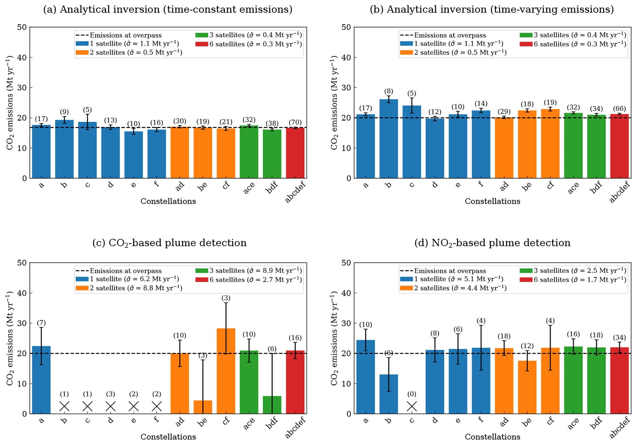
Figure 11Estimated annual emissions at satellite overpass for (a) analytical inversion and (b) mass-balance approach with CO2-based plume detection and (c) NO2-based plume detection for different constellation sizes. The number of overpasses with estimated emissions are shown in brackets. If the number of estimated emissions is too small for computing the seasonal cycle, values are marked with a cross. Error bars show the precision computed from the individual emission estimates at satellite overpass. The legend shows the mean error for each constellation size.
In contrast, estimating annual emissions with the mass balance is very difficult if only the CO2 observations are available for detecting the location of the plume. For a single satellite, the number of overpasses with successful emission estimates is too small to fit a seasonal cycle in nearly all cases, and even with two or three satellites the precision is low with about 8.8 Mt yr−1 (44 %). The situation significantly improves with additional NO2 observations. A single satellite can estimate annual emissions in five out of six cases with an average precision of 5.1 Mt yr−1 (26 %) due to the better temporal coverage. The average precision increases to 4.4 Mt yr−1 (22 %) and 2.5 Mt yr−1 (13 %) for constellations of two and three satellites, respectively. The annual emissions are slightly overestimated, because of low temporal coverage in winter and because the mass-balance approach is also sensitive to emissions outside of Berlin.
To estimate annual emissions accurately, it is necessary to resolve the real temporal variability of emissions. It should be noted that the temporal variability in the COSMO-GHG simulations used for generating the synthetic satellite observations likely underestimates the real variability. To generate temporally varying emissions in the simulations, we applied different diurnal, weekly and seasonal cycles to emissions from different sectors such as energy production, traffic and heating (Jähn et al., 2020). These fixed time profiles do not account for effects from meteorology and human drivers such as strikes, temporal traffic restrictions or holidays.
To resolve the temporal variability, a sufficiently large number of individual emission estimates is required. The number of estimates varies strongly between satellites due to the uneven distribution of cloud-free days. Even with the NO2 observations, it is still possible to have only four overpasses with estimated emissions per year with two satellites. Therefore, at least three satellites are likely necessary to get reliable estimates of the annual emissions. Higher temporal coverage can alternatively be achieved by increasing the swath width of the instrument.
Besides day-to-day variability of emissions, individual emission estimates are also only representative of emissions a few hours before the satellite overpass but not for the daily mean (Broquet et al., 2018). It would therefore still be necessary to apply a correction factor to obtain the annual mean emissions, which introduces an additional source of uncertainty not included in our estimate. In our simulation, the emissions during overpass are about 18 % higher than the daily mean, suggesting that the sampling bias would be of the same order of magnitude. However, this result is entirely driven by the sector-specific diurnal emission cycles prescribed in the simulations. If the diurnal cycle of emissions was known from other sources of information such as traffic counts, electricity demand and heating statistics, a correction of the sampling bias could be applied, but this correction would add an additional uncertainty. The uncertainty in current estimates of diurnal emission variations is very poorly known, which makes it difficult to derive uncertainties in diurnal cycle or precise knowledge about ratios between different periods of the day (Wang et al., 2020). Studies such as those of Nassar et al. (2013), Gurney et al. (2019) or Peylin et al. (2011) all present diurnal emission cycles from various sources of information but no analysis of uncertainties. The diurnal cycles presented in these studies are roughly in line with our estimate of a sampling bias of the order of 20 % with respect to the daily mean. Super et al. (2020) estimated uncertainties in the diurnal variation from uncertainties in activity data and emission factors, which, when applied to individual cities, would make it possible to better quantify the potential sampling bias in estimating annual emissions from sun-synchronous satellite observations in the future.
Finally, it should be noted that our results are representative for a city in mid-latitudes, where the temporal coverage is larger, as the satellites can pass over a city twice during the 11 d repeat cycle, whereas at the Equator only one satellite pass takes place per 11 d. The real temporal coverage is also strongly affected by the number of cloud-free observations in different latitudes.
In this study, a detailed analysis was conducted to investigate the potential of a constellation of CO2 satellites with imaging capability for quantifying the emissions of a large city like Berlin with or without additional NO2 measurements. The results are based on unique, 1-year-long very high resolution (1 km × 1 km) atmospheric CO2 simulations with the COSMO-GHG model, which accounts for anthropogenic and biospheric fluxes as realistically as possible. Synthetic satellite observations were generated for 2 km×2 km pixels from CO2 and NO2 model fields along the 250 km wide swaths of a constellation of up to six satellites.
The CO2 emissions of Berlin were quantified by two different methods to assess the range of uncertainties associated with different assumptions regarding the capabilities of atmospheric transport models. The emissions were quantified (1) by scaling the simulated CO2 tracer representing only emissions from Berlin to match the synthetic CO2 observations without the CO2 background field and (2) by applying a mass-balance approach that estimates the flux of CO2 through vertical control surfaces perpendicular to the direction of propagation of the detected plume. The second approach relies on a plume detection algorithm using either the CO2 or NO2 observations.
The first method assumes perfect knowledge of atmospheric transport and CO2 background fields. In this case, the uncertainty of the emission estimates is entirely driven by the ratio of instrument noise to the CO2 enhancements within the plume, which varies from case to case due to varying winds and cloud cover. The second method requires minimal model information except for an estimate of the mean wind speed within the plume, which would typically be obtained from a numerical weather prediction model analysis.
The analytical inversion estimated emissions with a SD of 3.0 to 4.2 Mt yr−1 for the low- to high-noise scenario and without a bias because systematic retrieval errors were not included here. The average number of successful estimates is 11.0 per satellite and year (range: 5–17). For the mass-balance approach 2.7 plumes per satellite (range: 1–7) were available on average with CO2-based plume detection and 5.7 plumes (range: 0–10) with the NO2-based plume detection due to the better signal-to-noise ratio of the NO2 observations. The mass-balance approach had a precision of about 10 Mt yr−1 for both CO2- and NO2-based plume detection.
The results obtained here can be compared with the Report for Mission Selection for CarbonSat that formulated a requirement of 7 Mt yr−1 uncertainty for single overpasses over a city with more than 35 Mt yr−1 (ESA, 2015). In our study, annual mean emissions of Berlin were much smaller (16.8 Mt yr−1) than assumed in previous studies due to the use of a dedicated inventory provided by the city of Berlin. Since emissions are higher during daytime than during nighttime, the emissions at satellite overpass time (11:30 LT) are 20.0 Mt yr−1, which is still significantly smaller than 35 Mt yr−1. For this magnitude of emissions the requirement of an uncertainty of 7 Mt yr−1 for single overpasses was clearly met under the assumption that the CO2 signature of the city plume and CO2 background field can be simulated perfectly. When using a mass-balance approach applied to the detected plumes, the requirement was almost met, irrespective of the uncertainty scenario used for the CO2 instrument.
The emissions estimated with the mass-balance approach can have significant systematic errors due to the challenge of estimating the CO2 background and the wind field accurately. Since the NO2 observations make it possible to not only detect the full city plume but also other small plumes in the vicinity, it is very helpful for estimating the CO2 background field more accurately and also for filtering out scenes with interfering plumes from other sources. Additional NO2 measurements on the same platform as the CO2 measurements are thus highly beneficial not only for detecting the plume but also for estimating the CO2 emissions. Furthermore, the analysis showed that CO2 emission estimates do not depend strongly on the precision of the CO2 observations for large plumes, for example, a city plume with more than 100 pixels. For these cases, a wider swath and somewhat reduced CO2 single sounding precision might be a reasonable trade-off. For smaller plumes, e.g., from power plants, a high precision of the CO2 observations is likely more relevant because of the small number of pixels contained in the plume.
Annual emissions were estimated by fitting a seasonal cycle to the individual estimates. The analytical inversion was able to estimate annual emissions with good precision with 1.1 Mt yr−1 (< 6 %) even with only one satellite, but this assumes perfect knowledge of the atmospheric transport. Estimating the annual emissions was more challenging with the mass-balance approach. If only the CO2 measurements were available for estimating emissions, one satellite was not sufficient for estimating annual emissions in most cases, because the number of individual estimates was too small. The precision was still low with two or three satellites (9 Mt yr−1 (44 %)).
If NO2 observations were available to detect the CO2 plumes, the annual emission could be estimated with one satellite in most cases (26 % precision) due to the better temporal coverage. The precision improved further to 4.4 Mt yr−1 (22 %) and 2.5 Mt yr−1 (13 %) with two and three satellites, respectively. It should be noted that the uncertainty in an annual mean estimate derived from satellite observations does not only depend on the number of individual plume estimates but also on the magnitude and correlation structure of the temporal variability of the emissions. Therefore, it is necessary to study how many individual emission estimates are required to constrain this variability assuming realistic temporal correlations.
Estimates of the city emissions are currently compiled in emission inventories based on activity data, energy statistics, emission factors and self-reported emissions. The uncertainties in total city emissions have a large range depending on data availability, and many cities do not even have an inventory (Gately and Hutyra, 2017). The characterization of uncertainties in inventories is a complex topic, since the characterization of uncertainties in the input parameters and thus the propagation of uncertainties is difficult (Super et al., 2020). The detailed emission inventory used for Berlin in our study reports only sector-specific uncertainties from which we estimate the uncertainty in total emissions to be around 25 %–30 % (AVISO GmbH and IE Leipzig, 2016). Our study therefore suggests that the CO2M mission will be able to quantify annual emissions of a city like Berlin with higher precision, even without knowledge about plume location and CO2 background from a transport model, if additional NO2 observations are available for detecting the plume and if the number of satellites is sufficiently large. With a population of 3.5 million, Berlin belongs to the 150 largest cities worldwide with more than 3 million inhabitants. The total population of these cities is 1.1 billion, which is roughly 15 % of the world's population (United Nations, 2018). According to the analysis of CO2 emission clusters by Wang et al. (2019), there are also about 150 urban areas worldwide that have similar or higher CO2 emissions than Berlin. Wang et al. (2020) showed that it might even be possible to constrain emissions of urban areas with emissions larger than 8 Mtyr−1, which would be about 300 cities.
Combining the mass-balance approach with additional information from models and other observations could further improve the accuracy of the CO2 emission estimates if they would help to constrain critical aspects of the method such as the position of the plume or the wind speed. The European CO2 emission monitoring and verification support system, as envisioned to be implemented in the Copernicus program, would use the CO2M observations together with information from atmospheric transport models. Since spatial mismatches between real and simulated plumes may lead to large errors in the emission estimates, the system will have to account for uncertainties in simulated atmospheric transport. One way forward could thus be to develop an advanced data assimilation system able to extract wind information directly from the plume observation as demonstrated, for example, by Allen et al. (2013) for a 4D-Var ozone assimilation system. Since the shape and extent of the plume can be imaged more accurately from the NO2 observations, the NO2 measurements could be a very useful source of information in such a data assimilation system.
XCO2, CO and NO2 columns of all simulated tracers are available both as 2-D fields and as synthetic satellite products (Kuhlmann et al., 2020). The code used in the publication is available on request and will be published on the GitLab group of the Laboratory for Air Pollution/Environmental Technology (https://gitlab.com/empa503, last access: 30 November 2020, Empa, 2020) upon completion of the SMARTCARB project.
The supplement related to this article is available online at: https://doi.org/10.5194/amt-13-6733-2020-supplement.
GK developed, implemented, applied and evaluated the methods for estimating CO2 emissions and wrote the manuscript with input from all co-authors. DB supervised and led the project SMARTCARB. GB followed the project as an external advisor and contributed critical input to the manuscript. YM accompanied the study as an ESA project officer and provided critical inputs and reviews during all phases of the project.
The author declares that there is no conflict of interest.
We acknowledge funding of the project SMARTCARB by the European Space Agency (ESA) and support by the EU Horizon-2020 project CHE. The views expressed here can in no way be taken to reflect the official opinion of ESA. The work was supported by a grant from the Swiss National Supercomputing Centre (CSCS) under project ID s862.
This research has been supported by the European Space Agency (grant no. 4000119599/16/NL/FF/mg), the European Commission, H2020 CO2 Human Emissions (CHE (grant no. 776186)), and the Swiss National Supercomputing Centre (project ID s862).
This paper was edited by Daniela Famulari and reviewed by two anonymous referees.
Agustí-Panareda, A., Massart, S., Chevallier, F., Boussetta, S., Balsamo, G., Beljaars, A., Ciais, P., Deutscher, N. M., Engelen, R., Jones, L., Kivi, R., Paris, J.-D., Peuch, V.-H., Sherlock, V., Vermeulen, A. T., Wennberg, P. O., and Wunch, D.: Forecasting global atmospheric CO2, Atmos. Chem. Phys., 14, 11959–11983, https://doi.org/10.5194/acp-14-11959-2014, 2014. a
Allen, D. R., Hoppel, K. W., Nedoluha, G. E., Kuhl, D. D., Baker, N. L., Xu, L., and Rosmond, T. E.: Limitations of wind extraction from 4D-Var assimilation of ozone, Atmos. Chem. Phys., 13, 3501–3515, https://doi.org/10.5194/acp-13-3501-2013, 2013. a
AVISO GmbH and IE Leipzig: Erstellung der Berliner Emissionskataster Industrie, Gebäudeheizung, sonstiger Verkehr, Kleingewerbe, sonstige Quellen, Baustellen – Schlussbericht Juni 2016, Tech. rep., available at: https://www.berlin.de/senuvk/umwelt/luftqualitaet/de/emissionen/download/Endbericht_Emissionkataster_2015.pdf (last access: 30 November 2020), 2016. a, b
Baldauf, M., Seifert, A., Forstner, J., Majewski, D., Raschendorfer, M., and Reinhardt, T.: Operational convective-scale numerical weather prediction with the COSMO model: description and sensitivities, Mon. Weather Rev., 139, 3887–3905, https://doi.org/10.1175/Mwr-D-10-05013.1, 2011. a
Beirle, S., Boersma, K. F., Platt, U., Lawrence, M. G., and Wagner, T.: Megacity Emissions and Lifetimes of Nitrogen Oxides Probed from Space, Science, 333, 1737–1739, https://doi.org/10.1126/science.1207824, 2011. a, b
Beirle, S., Borger, C., Dörner, S., Li, A., Hu, Z., Liu, F., Wang, Y., and Wagner, T.: Pinpointing nitrogen oxide emissions from space, Sci. Adv., 5, eaax9800, https://doi.org/10.1126/sciadv.aax9800, 2019. a
Boersma, K. F., Eskes, H. J., Dirksen, R. J., van der A, R. J., V Boersma, K. F., Eskes, H. J., Dirksen, R. J., van der A, R. J., Veefkind, J. P., Stammes, P., Huijnen, V., Kleipool, Q. L., Sneep, M., Claas, J., Leitão, J., Richter, A., Zhou, Y., and Brunner, D.: An improved tropospheric NO2 column retrieval algorithm for the Ozone Monitoring Instrument, Atmos. Meas. Tech., 4, 1905–1928, https://doi.org/10.5194/amt-4-1905-2011, 2011. a
Bovensmann, H., Buchwitz, M., Burrows, J. P., Reuter, M., Krings, T., Gerilowski, K., Schneising, O., Heymann, J., Tretner, A., and Erzinger, J.: A remote sensing technique for global monitoring of power plant CO2 emissions from space and related applications, Atmos. Meas. Tech., 3, 781–811, https://doi.org/10.5194/amt-3-781-2010, 2010. a
Broquet, G., Bréon, F.-M., Renault, E., Buchwitz, M., Reuter, M., Bovensmann, H., Chevallier, F., Wu, L., and Ciais, P.: The potential of satellite spectro-imagery for monitoring CO2 emissions from large cities, Atmos. Meas. Tech., 11, 681–708, https://doi.org/10.5194/amt-11-681-2018, 2018. a, b, c, d
Brunner, D., Kuhlmann, G., Marshall, J., Clément, V., Fuhrer, O., Broquet, G., Löscher, A., and Meijer, Y.: Accounting for the vertical distribution of emissions in atmospheric CO2 simulations, Atmos. Chem. Phys., 19, 4541–4559, https://doi.org/10.5194/acp-19-4541-2019, 2019. a, b, c
Buchwitz, M., Reuter, M., Bovensmann, H., Pillai, D., Heymann, J., Schneising, O., Rozanov, V., Krings, T., Burrows, J. P., Boesch, H., Gerbig, C., Meijer, Y., and Löscher, A.: Carbon Monitoring Satellite (CarbonSat): assessment of atmospheric CO2 and CH4 retrieval errors by error parameterization, Atmos. Meas. Tech., 6, 3477–3500, https://doi.org/10.5194/amt-6-3477-2013, 2013. a
C40 cities: 27 Cities Have Reached Peak Greenhouse Gas Emissions whilst Populations Increase and Economies Grow, Press release, available at: https://www.c40.org/press_releases/27-cities-have-reached-peak-greenhouse-gas-emissions-whilst- -populations-increase-and-economies-grow (last access: 30 November 2020), 2018. a
Ciais, P., Crisp, D., v. d. Gon, H., Engelen, R., Heimann, M., Janssens-Maenhout, G., Rayner, P., and Scholze, M.: Towards a European Operational Observing System to Monitor Fossil CO2 emissions – Final Report from the expert group, Copernicus Climate Change Service, Report, European Commission, Brussels, 2015. a
Düring, I., Bächlin, W., Ketzel, M., Baum, A., Friedrich, U., and Wurzler, S.: A new simplified NO/NO2 conversion model under consideration of direct NO2-emissions, Meteorol. Z., 20, 67–73, https://doi.org/10.1127/0941-2948/2011/0491, 2011. a
Empa – Laboratory for Air Pollution/Environmental Technology – GitLab group “empa503”: https://gitlab.com/empa503, last access: 30 November 2020. a
ESA: Report for mission selection: CarbonSat, ESA SP-1330/1 (2 volume series), Report, ESA communications, Noordwijk, 2015. a
Fioletov, V. E., McLinden, C. A., Krotkov, N., and Li, C.: Lifetimes and emissions of SO2 from point sources estimated from OMI, Geophys. Res. Lett., 42, 1969–1976, https://doi.org/10.1002/2015GL063148, 2015. a
Flemming, J., Huijnen, V., Arteta, J., Bechtold, P., Beljaars, A., Blechschmidt, A.-M., Diamantakis, M., Engelen, R. J., Gaudel, A., Inness, A., Jones, L., Josse, B., Katragkou, E., Marecal, V., Peuch, V.-H., Richter, A., Schultz, M. G., Stein, O., and Tsikerdekis, A.: Tropospheric chemistry in the Integrated Forecasting System of ECMWF, Geosci. Model Dev., 8, 975–1003, https://doi.org/10.5194/gmd-8-975-2015, 2015. a
Gately, C. K. and Hutyra, L. R.: Large Uncertainties in Urban-Scale Carbon Emissions, J. Geophys. Res.-Atmos., 122, 11,242–11,260, https://doi.org/10.1002/2017JD027359, 2017. a
Gurney, K. R., Patarasuk, R., Liang, J., Song, Y., O'Keeffe, D., Rao, P., Whetstone, J. R., Duren, R. M., Eldering, A., and Miller, C.: The Hestia fossil fuel CO2 emissions data product for the Los Angeles megacity (Hestia-LA), Earth Syst. Sci. Data, 11, 1309–1335, https://doi.org/10.5194/essd-11-1309-2019, 2019. a
Houweling, S., Landgraf, J., van Heck, H., Vlemmix, T., and Tao, W.: AEROCARB – Study on use of aerosol information for estimating fossil CO2 emissions, Final report: Synthesis and Recommendation, Tech. rep., ESA study contract RFP/3-14860/17/NL/FF/gp, SRON – Netherlands Institute for Space Research Location: Utrecht, 2019. a
International Energy Agency: Implications of the reference scenario for the global climate, World Energy Outlook, IEA, Paris, 381–406, available at: https://www.iea.org/reports/world-energy-outlook-2008 (last access: 30 November 2020), 2008. a
Jähn, M., Kuhlmann, G., Mu, Q., Haussaire, J.-M., Ochsner, D., Osterried, K., Clément, V., and Brunner, D.: An online emission module for atmospheric chemistry transport models: implementation in COSMO-GHG v5.6a and COSMO-ART v5.1-3.1, Geosci. Model Dev., 13, 2379–2392, https://doi.org/10.5194/gmd-13-2379-2020, 2020. a
Janssens-Maenhout, G., Pinty, B., Dowell, M., Zunker, H., Andersson, E., Balsamo, G., Bézy, J.-L., Brunhes, T., Bösch, H., Bojkov, B., Brunner, D., Buchwitz, M., Crisp, D., Ciais, P., Counet, P., Dee, D., Denier van der Gon, H., Dolman, H., Drinkwater, M., Dubovik, O., Engelen, R., Fehr, T., Fernandez, V., Heimann, M., Holmlund, K., Houweling, S., Husband, R., Juvyns, O., Kentarchos, A., Landgraf, J., Lang, R., Löscher, A., Marshall, J., Meijer, Y., Nakajima, M., Palmer, P., Peylin, P., Rayner, P., Scholze, M., Sierk, B., Tamminen, J., and Veefkind, P.: Towards an operational anthropogenic CO2 emissions monitoring and verification support capacity, B. Am. Meteorol. Soc., 101, E1439–E1451, https://doi.org/10.1175/BAMS-D-19-0017.1, 2020. a
Klausner, T., Mertens, M., Huntrieser, H., Galkowski, M., Kuhlmann, G., Baumann, R., Fiehn, A., Jöckel, P., Pühl, M., and Roiger, A.: Urban greenhouse gas emissions from the Berlin area: A case study using airborne CO2 and CH4 in situ observations in summer 2018, Elem. Sci. Anth., 8, 15, https://doi.org/10.1525/elementa.411, 2019. a
Krings, T., Gerilowski, K., Buchwitz, M., Hartmann, J., Sachs, T., Erzinger, J., Burrows, J. P., and Bovensmann, H.: Quantification of methane emission rates from coal mine ventilation shafts using airborne remote sensing data, Atmos. Meas. Tech., 6, 151–166, https://doi.org/10.5194/amt-6-151-2013, 2013. a
Kuenen, J. J. P., Visschedijk, A. J. H., Jozwicka, M., and Denier van der Gon, H. A. C.: TNO-MACC_II emission inventory; a multi-year (2003–2009) consistent high-resolution European emission inventory for air quality modelling, Atmos. Chem. Phys., 14, 10963–10976, https://doi.org/10.5194/acp-14-10963-2014, 2014. a
Kuhlmann, G., Broquet, G., Marshall, J., Clément, V., Löscher, A., Meijer, Y., and Brunner, D.: Detectability of CO2 emission plumes of cities and power plants with the Copernicus Anthropogenic CO2 Monitoring (CO2M) mission, Atmos. Meas. Tech., 12, 6695–6719, https://doi.org/10.5194/amt-12-6695-2019, 2019a. a, b, c, d, e, f
Kuhlmann, G., Clément, V., Marschall, J., Fuhrer, O., Broquet, G., Schnadt-Poberaj, C., Löscher, A., Meijer, Y., and Brunner, D.: SMARTCARB – Use of Satellite Measurements of Auxiliary Reactive Trace Gases for Fossil Fuel Carbon Dioxide Emission Estimation, Final report of ESA study contract no 4000119599/16/NL/FF/mg, Tech. rep., Empa, Swiss Federal Laboratories for Materials Science and Technology, Dübendorf, Switzerland, https://doi.org/10.5281/zenodo.4034266, 2019b. a
Kuhlmann, G., Clément, V., Marshall, J., Fuhrer, O., Broquet, G., Schnadt-Poberaj, C., Löscher, A., Meijer, Y., and Brunner, D.: Synthetic XCO2, CO and NO2 observations for the CO2M and Sentinel-5 satellites, Data set, Zenodo, https://doi.org/10.5281/zenodo.4048228, 2020. a
Laughner, J. L. and Cohen, R. C.: Direct observation of changing NOx lifetime in North American cities, Science, 366, 723–727, https://doi.org/10.1126/science.aax6832, 2019. a
Liu, Y., Gruber, N., and Brunner, D.: Spatiotemporal patterns of the fossil-fuel CO2 signal in central Europe: results from a high-resolution atmospheric transport model, Atmos. Chem. Phys., 17, 14145–14169, https://doi.org/10.5194/acp-17-14145-2017, 2017. a
Lorente, A., Boersma, K., Eskes, H., Veefkind, J., Van Geffen, J., de Zeeuw, M., van der Gon, H. D., Beirle, S., and Krol, M.: Quantification of nitrogen oxides emissions from build-up of pollution over Paris with TROPOMI, Sci. Rep.-UK, 9, 1–10, https://doi.org/10.1038/s41598-019-56428-5, 2019. a
Mahadevan, P., Wofsy, S. C., Matross, D. M., Xiao, X., Dunn, A. L., Lin, J. C., Gerbig, C., Munger, J. W., Chow, V. Y., and Gottlieb, E. W.: A satellite-based biosphere parameterization for net ecosystem CO2 exchange: Vegetation Photosynthesis and Respiration Model (VPRM), Global Biogeochem. Cy., 22, https://doi.org/10.1029/2006GB002735, 2008. a
Nassar, R., Napier-Linton, L., Gurney, K. R., Andres, R. J., Oda, T., Vogel, F. R., and Deng, F.: Improving the temporal and spatial distribution of CO2 emissions from global fossil fuel emission data sets, J. Geophys. Res.-Atmos., 118, 917–933, https://doi.org/10.1029/2012JD018196, 2013. a
Nassar, R., Hill, T. G., McLinden, C. A., Wunch, D., Jones, D. B. A., and Crisp, D.: Quantifying CO2 Emissions From Individual Power Plants From Space, Geophys. Res. Lett., 44, 10045–10053, https://doi.org/10.1002/2017GL074702, 2017. a
Peylin, P., Houweling, S., Krol, M. C., Karstens, U., Rödenbeck, C., Geels, C., Vermeulen, A., Badawy, B., Aulagnier, C., Pregger, T., Delage, F., Pieterse, G., Ciais, P., and Heimann, M.: Importance of fossil fuel emission uncertainties over Europe for CO2 modeling: model intercomparison, Atmos. Chem. Phys., 11, 6607–6622, https://doi.org/10.5194/acp-11-6607-2011, 2011. a
Pillai, D., Buchwitz, M., Gerbig, C., Koch, T., Reuter, M., Bovensmann, H., Marshall, J., and Burrows, J. P.: Tracking city CO2 emissions from space using a high-resolution inverse modelling approach: a case study for Berlin, Germany, Atmos. Chem. Phys., 16, 9591–9610, https://doi.org/10.5194/acp-16-9591-2016, 2016. a, b, c
Pinty, B., Janssens-Maenhout, G., Dowell, M., Zunker, H., Brunhe, T., Ciais, P., Dee, D., van der Gon, H. D., Dolman, H., Drinkwater, M., Engelen, R., Heimann, M., Holmlund, K., Husband, R., Kentarchos, A., Meijer, Y., Palmer, P., and Scholze, M.: An Operational Anthropogenic CO2 Emissions Monitoring & Verification Support capacity – Baseline Requirements, Model Components and Functional Architecture, Report, available at: https://www.copernicus.eu/sites/default/files/2019-09/CO2_Red_Report_2017.pdf (last access: 30 November 2020), 2017. a
Pitt, J. R., Allen, G., Bauguitte, S. J.-B., Gallagher, M. W., Lee, J. D., Drysdale, W., Nelson, B., Manning, A. J., and Palmer, P. I.: Assessing London CO2, CH4 and CO emissions using aircraft measurements and dispersion modelling, Atmos. Chem. Phys., 19, 8931–8945, https://doi.org/10.5194/acp-19-8931-2019, 2019. a
Reuter, M., Buchwitz, M., Schneising, O., Krautwurst, S., O'Dell, C. W., Richter, A., Bovensmann, H., and Burrows, J. P.: Towards monitoring localized CO2 emissions from space: co-located regional CO2 and NO2 enhancements observed by the OCO-2 and S5P satellites, Atmos. Chem. Phys., 19, 9371–9383, https://doi.org/10.5194/acp-19-9371-2019, 2019. a, b, c
Rockström, J., Gaffney, O., Rogelj, J., Meinshausen, M., Nakicenovic, N., and Schellnhuber, H. J.: A roadmap for rapid decarbonization, Science, 355, 1269–1271, https://doi.org/10.1126/science.aah3443, 2017. a
Sharp, E., Dodds, P., Barrett, M., and Spataru, C.: Evaluating the accuracy of CFSR reanalysis hourly wind speed forecasts for the UK, using in situ measurements and geographical information, Renew. Energ., 77, 527–538, https://doi.org/10.1016/j.renene.2014.12.025, 2015. a
Sierk, B., Bézy, J.-L., Löscher, A., and Meijer, Y.: The European CO2 Monitoring Mission: observing anthropogenic greenhouse gas emissions from space, SPIE, 237–250, https://doi.org/10.1117/12.2535941, 2019. a, b
Super, I., Dellaert, S. N. C., Visschedijk, A. J. H., and Denier van der Gon, H. A. C.: Uncertainty analysis of a European high-resolution emission inventory of CO2 and CO to support inverse modelling and network design, Atmos. Chem. Phys., 20, 1795–1816, https://doi.org/10.5194/acp-20-1795-2020, 2020. a, b
Turnbull, J. C., Karion, A., Davis, K. J., Lauvaux, T., Miles, N. L., Richardson, S. J., Sweeney, C., McKain, K., Lehman, S. J., Gurney, K. R., Patarasuk, R., Liang, J., Shepson, P. B., Heimburger, A., Harvey, R., and Whetstone, J.: Synthesis of Urban CO2 Emission Estimates from Multiple Methods from the Indianapolis Flux Project (INFLUX), Environ. Sci. Technol., 53, 287–295, 2018. a
United Nations: World Urbanization Prospects: The 2018 Revision, Department of Economic and Social Affairs, Population Division, online edn., available at: https://population.un.org/wup/ (last access: 30 November 2020), 2018. a
Wang, Y., Ciais, P., Broquet, G., Bréon, F.-M., Oda, T., Lespinas, F., Meijer, Y., Loescher, A., Janssens-Maenhout, G., Zheng, B., Xu, H., Tao, S., Gurney, K. R., Roest, G., Santaren, D., and Su, Y.: A global map of emission clumps for future monitoring of fossil fuel CO2 emissions from space, Earth Syst. Sci. Data, 11, 687–703, https://doi.org/10.5194/essd-11-687-2019, 2019. a
Wang, Y., Broquet, G., Bréon, F.-M., Lespinas, F., Buchwitz, M., Reuter, M., Meijer, Y., Loescher, A., Janssens-Maenhout, G., Zheng, B., and Ciais, P.: PMIF v1.0: assessing the potential of satellite observations to constrain CO2 emissions from large cities and point sources over the globe using synthetic data, Geosci. Model Dev., 13, 5813–5831, https://doi.org/10.5194/gmd-13-5813-2020, 2020. a, b, c
Wu, D., Lin, J. C., Oda, T., and Kort, E. A.: Space-based quantification of per capita CO2 emissions from cities, Environ. Res. Lett., 15, 035004, https://doi.org/10.1088/1748-9326/ab68eb, 2020. a
Zheng, B., Chevallier, F., Ciais, P., Broquet, G., Wang, Y., Lian, J., and Zhao, Y.: Observing carbon dioxide emissions over China's cities and industrial areas with the Orbiting Carbon Observatory-2, Atmos. Chem. Phys., 20, 8501–8510, https://doi.org/10.5194/acp-20-8501-2020, 2020. a
- Article
(6477 KB) - Full-text XML