the Creative Commons Attribution 4.0 License.
the Creative Commons Attribution 4.0 License.
 | 16 Dec 2020
Probabilistic analysis of ambiguities in radar echo direction of arrival from meteors
Johan Kero
Meteors and hard targets produce coherent radar echoes. If measured with an interferometric radar system, these echoes can be used to determine the position of the target through finding the direction of arrival (DOA) of the incoming echo onto the radar. Depending on the spatial configuration of radar-receiving antennas and their individual gain patterns, there may be an ambiguity problem when determining the DOA of an echo. Radars that are theoretically ambiguity-free are known to still have ambiguities that depend on the total radar signal-to-noise ratio (SNR). In this study, we investigate robust methods which are easy to implement to determine the effect of ambiguities on any hard target DOA determination by interferometric radar systems. We apply these methods specifically to simulate four different radar systems measuring meteor head and trail echoes, using the multiple signal classification (MUSIC) DOA determination algorithm. The four radar systems are the Middle And Upper Atmosphere (MU) radar in Japan, a generic Jones 2.5λ specular meteor trail radar configuration, the Middle Atmosphere Alomar Radar System (MAARSY) radar in Norway and the Program of the Antarctic Syowa Mesosphere Stratosphere Troposphere Incoherent Scatter (PANSY) radar in the Antarctic. We also examined a slightly perturbed Jones 2.5λ configuration used as a meteor trail echo receiver for the PANSY radar. All the results are derived from simulations, and their purpose is to grant understanding of the behaviour of DOA determination. General results are as follows: there may be a region of SNRs where ambiguities are relevant; Monte Carlo simulation determines this region and if it exists; the MUSIC function peak value is directly correlated with the ambiguous region; a Bayesian method is presented that may be able to analyse echoes from this region; the DOA of echoes with SNRs larger than this region are perfectly determined; the DOA of echoes with SNRs smaller than this region completely fail to be determined; the location of this region is shifted based on the total SNR versus the channel SNR in the direction of the target; and asymmetric subgroups can cause ambiguities, even for ambiguity-free radars. For a DOA located at the zenith, the end of the ambiguous region is located at 17 dB SNR for the MU radar and 3 dB SNR for the PANSY radar. The Jones radars are usually used to measure specular trail echoes far from zenith. The ambiguous region for a DOA at 75.5∘ elevation and 0∘ azimuth ends at 12 dB SNR. Using the Bayesian method, it may be possible to analyse echoes down to 4 dB SNR for the Jones configuration when given enough data points from the same target. The PANSY meteor trail echo receiver did not deviate significantly from the generic Jones configuration. The MAARSY radar could not resolve arbitrary DOAs sufficiently well enough to determine a stable region. However, if the DOA search is restricted to 70∘ elevation or above by assumption, stable DOA determination occurs above 15 dB SNR.
- Article
(8546 KB) - Full-text XML
- BibTeX
- EndNote


Radar systems are a vital part of current research infrastructure. They are used for a wide variety of novel (e.g. Sato et al., 2014; Kero et al., 2012b; McCrea et al., 2015) and routine remote sensing observations (e.g. Hocking, 2005, and references therein). One subset of these observations is objects and phenomena in the atmosphere that produce coherent radar echoes. Meteor head and trail echoes, satellite and space debris echoes, polar mesospheric echoes, field-aligned irregularities and many more phenomena fall under this category. However, to discern the position and motion of these radar targets, interferometric or multi-static radar systems must be used.
When determining the position of an object by interferometry, there is an ambiguity problem (Schmidt, 1986). The position is determined by finding the direction of arrival (DOA) of the incoming echo onto the radar. Depending on the spatial configuration of the receiving antennas and their individual gain patterns, the voltage response can be the same for several different plane wave DOAs, thereby making it impossible to determine the correct direction. This problem is general for all DOA determinations made by radar systems with interferometry baselines longer than half a wavelength. In this study, it is put in the context of meteor head and trail echo observations.
Every day the Earth's atmosphere is bombarded by billions of dust-sized particles and larger pieces of material from space. This incoming material gives us a unique opportunity to examine the motion and population of small bodies in the solar system (e.g. Vaubaillon et al., 2005a, b; Kastinen and Kero, 2017). Objects with sizes between 100 µm and 1 m that move in interplanetary space are called meteoroids. Meteoroids originate from comets and asteroids; they are abundant and can have high velocities (Whipple, 1951). When meteoroids enter the atmosphere, they burn up causing a phenomenon known as a meteor (Ceplecha et al., 1998). The meteor itself can be divided into two parts that function as hard targets, namely the dense plasma co-moving with the ablating meteoroid and the trail of diffusing plasma left in the atmosphere. These generate the meteor head and trail echoes.
Meteor trail plasma drifts with the ambient atmosphere. The drift velocity is therefore a measure of the neutral wind at the observation altitude. The typical ablation altitude where meteor phenomena occur lies between 70 and 130 km. This region is characterised by variability driven by atmospheric tides and planetary and smaller-scale gravity waves. Specular meteor trail radars have become widespread scientific instruments for studying atmospheric dynamics deployed at locations covering latitudes from Antarctica to the Arctic Svalbard (Kero et al., 2019). To calculate the neutral wind, the DOA of the specular echo must be determined.
Due to the altitude distribution of meteor phenomena, the far field approximation is almost always valid, which means that an incoming echo can be modelled as a plane wave (Kildal, 2015). The only exception is the Arecibo radio telescope due to its 300 m diameter large spherical reflector at a 430 MHz operating frequency. Using an interferometric radar system to determine the DOA of a meteor head echo as a function of time allows the construction of a meteoroid trajectory (e.g. Kero et al., 2012b; Jones et al., 2005, 1998; Szasz et al., 2008; Chau and Woodman, 2004; Close et al., 2000). This trajectory is the base for computing the meteor position, meteoroid velocity and radar cross section and for reconstructing the original meteoroid solar system orbit.
There are analytical methods for determining all the ambiguities present in a radar system, although these scale poorly and have several restrictions (Kastinen, 2018; Schmidt, 1986). Systems that have no theoretical ambiguities also suffer from ambiguous DOA solutions due to noise (Kastinen, 2018; Jones et al., 1998). These so-called noise-induced ambiguities are not multiple solutions to the DOA determination. Instead, the DOA determination output becomes a stochastic variable that is no longer centred on the true DOA but is spread out between several different DOA solutions with similar radar responses. Thus, when determining the DOA of a noisy signal, there is a probability of misclassifying the DOA. This misclassification probability is separate from the DOA error introduced by the noise that is usually the focus in measurement pipelines (Kero et al., 2012b) and depends on the signal-to-noise ratio (SNR) of the received signal. In these cases, point spread functions (PSFs) have be used to determine the morphology of expected ambiguities. However, these do not relate SNR to DOA misclassification probabilities (Chau and Clahsen, 2019). The morphology of the PSF may also depend on the input DOA itself (further discussed in Appendix B).
The existence of head echo events, such as the one illustrated in Fig. 1, is what prompted this study. This meteor is seemingly jumping from place to place in the sky, even though the range and line of sight velocity was well determined. This was a special case among thousands of other successful and validated measurements using the same analysis and system. Hence, the goal of this study is to understand enough about DOA determination behaviour to investigate these types of events, especially today when analysis is automated and databases can contain millions of events (Campbell-Brown, 2019). If even a small fraction of these events stand out as interesting but are the result of ambiguities or other artefacts, consequent research can be negatively influenced. On the other hand, given strange results, large portions of data may be discarded when in fact some are not a consequence of ambiguities or algorithmic errors (Schult et al., 2013). Having a good understanding of DOA determination behaviour may also allow us to analyse events with lower SNR than at present (Jones et al., 1998).
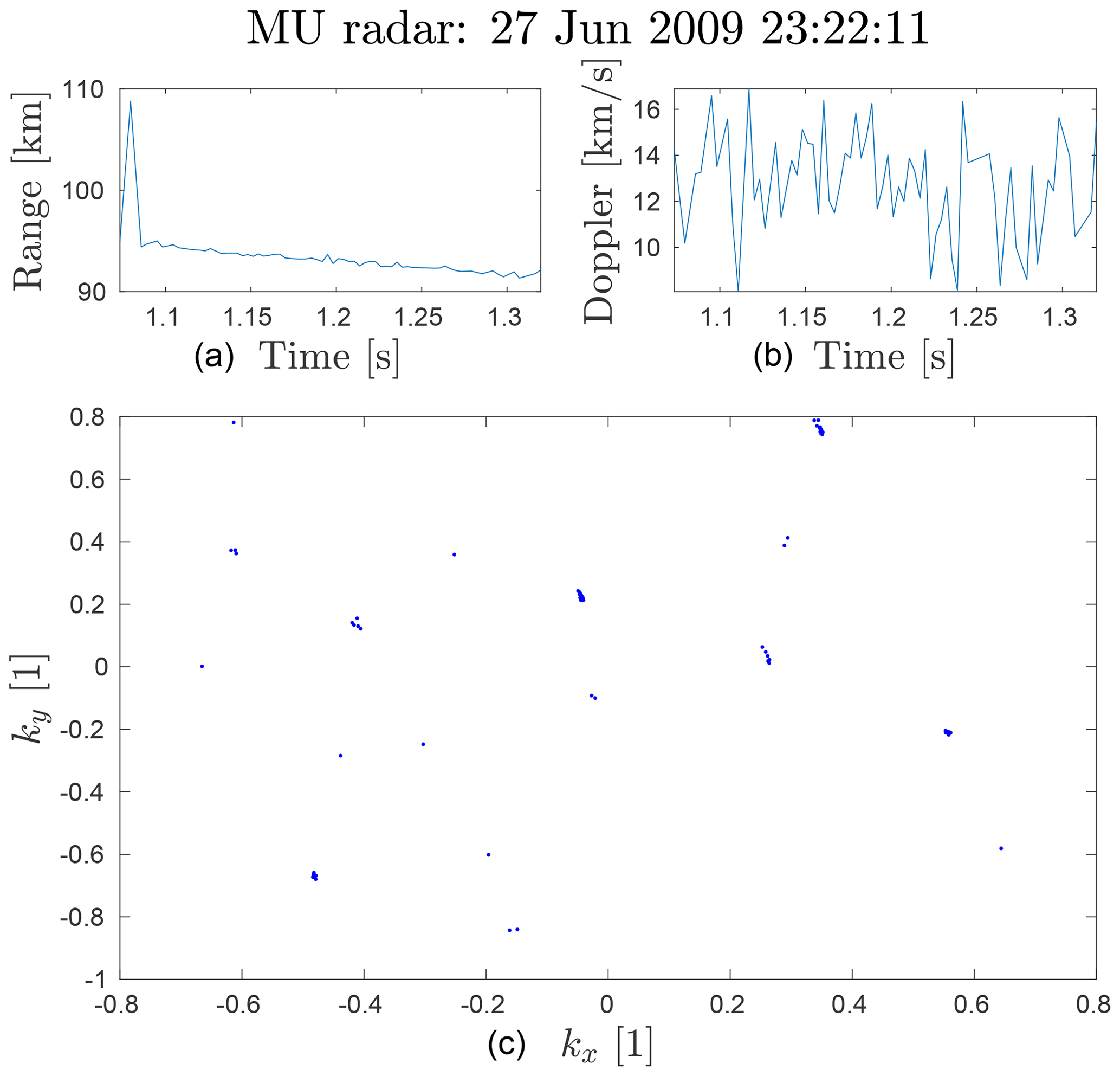
Figure 1Example meteor head event measured with the MU radar which seems ambiguous. Panel (a) is the one-way range, panel (b) is the line-of-sight velocity and panel (c) is the normalised wave vector ground projection. The wave vector +y axis is aligned with north and the +x axis with the east. The SNR varied between 8 and 16 dB for this event. The goal of this paper is to understand enough about DOA determination behaviour to investigate these types of events.
There are no methods, to our knowledge, for resolving noise-induced ambiguities in DOA determinations or for determining the probability of misclassification. We have therefore extended upon the study performed in Kastinen (2018).
In Sect. 2 we present a numerical method for determining the DOA ambiguities, which works irrespective of whether the ambiguities are noise induced or not. The method can be applied on arbitrary radar systems and experiences no large scaling problems with system complexity. It also allows for arbitrary receiver models to be used.
Section 3 provides an overview of how we have applied the multiple signal classification (MUSIC) algorithm. The MUSIC method allows for an arbitrary sensor response model and can thus be applied on any radar system.
We have focused on radars measuring the meteor phenomena. However, the analysis methods applied are usable on any kind of interferometric hard-target detections made by radars. The radars that we have applied these techniques on are described in Sect. 4, and the results are presented in Sect. 5. The results for each system are also discussed in the respective subsection. Finally, we conclude the results and discuss the overall results in Sect. 6.
2.1 Ambiguities
To find the ambiguities present when determining the DOA, we need a radar sensor response model Φ. A model for a radar with antennas at locations rj with individual complex gain functions gj(k), receiving a plane wave of amplitude A, is described by the following:
Here, k is the wave vector of the incoming plane wave. We denote the inner product of a space X by , i.e. is the real 3D inner product. In the case of radar systems with sub-arrays, the gj(k) functions can be defined as follows:
where γjl(k) are the antennas' individual gain functions, and ρjl are the sub-array antenna locations. In this case, the rj locations are the geometric centres of the sub-arrays, i.e. the phase centres. In all radar systems we consider, the same type of antennas are used throughout the system. Also, we are not aware of any studies that find variability in individual antenna gain patterns due to effects like mutual coupling for the radar systems we have investigated. As such, we can use a common function for all antennas γjl(k)=γ(k).
Usually, the wave amplitude A is unknown, and the DOA determination algorithm should therefore be invariant of signal amplitude . As such, our definition of an ambiguity should also be invariant of signal amplitude.
In the pursuit of an analytical solution, Kastinen (2018) was unable to include the variable gain patterns gi of the radar channels in the formula for finding ambiguities. The calculation method presented there scaled badly with the number of channels in the system and was not invariant to signal amplitude. We have resolved these issues, thereby allowing for any model Φ to be used, by numerically finding ambiguities on a case-by-case basis.
The normalised sensor response model is written as follows:
Ambiguities are formed when the following occurs:
Exactly what the conditions “approximate to” and “not approximate to” mean in this definition needs to be decided on a case-by-case basis as explained further below. The reason for this specific definition will also be covered further below. Equation (4) is invariant to the individual antenna gain γ(k). Thus, we may define γ(k)=1 for all examined radar systems.
We call an ambiguity perfect, i.e. unambiguous DOA determination is impossible even at infinite SNR, if .
We define a set of ambiguities to k0 as the vectors k that fulfil Eq. (4), as follows:
It is important to note that it is not sufficient to calculate the set of ambiguities for only one k0, as this set may not display the same pattern as the set for another direction k1.
Following the definition in Eq. (4), an indicator function of ambiguities is the normalised sensor response inner product, as follows:
There are several other ways to define ambiguities. The requirement is that the definition is invariant of the sensor response norm and is to a constant phase offset in all dimensions; which definition to use depends on the behaviour of the DOA determination algorithm. One important property of algorithms is whether or not they preserve orientation with respect to . Neither the MUSIC algorithm (see Sect. 3) nor Eq. (6) preserve orientation. The latter is visualised by imagining the inner product as a scalar projection of onto . This projection contains the orientation of with respect to . For real vector spaces, the orientation is expressed in terms of + or −, while for complex vector spaces it is expressed in the form of the phase of the complex number. The orientation is disregarded in Eq. (6) when we apply the absolute value.
One of several possible other formulations is using a distance function. The definition would then be . This is not invariant to the orientation. One can also create a function that is not invariant by using the inner product defined in Eq. (6) but not applying the absolute value, i.e. . These equations and Eq. (6) often, but not always, produce equivalent solution sets given an ambiguity search, depending on search algorithm configurations. We have elected to use Eq. (6) as an ambiguity indicator function since it describes the behaviour of MUSIC well.
If the set Ω(k0) is finite, the indicator function d must have peaks with a single point top at every k in Ω(k0). These peaks k are separated from k0 and have heights d that are used to decide if they should be included in the ambiguity set Ω(k0) or not. As the peaks identify ambiguities, we have implemented a scattered gradient ascent method to determine the ambiguity set Ω for a given k0. The step-by-step method is as follows:
-
Define a source wave direction k0.
-
Generate a set of n start wave vectors {ai} distributed (e.g. uniformly) on the hemisphere.
-
Do a gradient ascent search, using the gradient of Eq. (6), for each start wave vector ai.
-
Collect the peak locations {bi} and peak heights {d(bi)}.
-
Remove duplicate results yielding the set of all ambiguities and their peaks {ki,d(ki)}.
This method can be used with any sensor response model to find ambiguities. After the set {ki,d(ki)} is acquired, it is necessary to filter the set based on what is deemed approximate and not approximate as per Eq. (5). This is done based on a minimum peak height ϵd and a minimum separation from k0. The filtering prevents the inclusion of ambiguities that only appear at unrealistically low SNRs. We will from here on denote this filtered set of ambiguities by Ω(k0)={ki}.
An important factor to note is that these ambiguities are not necessarily transitive relations. They are only transitive when the indicator function is 1, i.e. they occupy the same point in sensor response space. The intransitive relation means that, for d<1, if k1 is ambiguous with k2 and k2 is ambiguous with k3, k1 does not have to be ambiguous with k3.
2.2 Noise
All the radar systems considered in this study have operating frequencies in the very high frequency (30–300 MHz) range. In this range, the galactic background radiation dominates the noise (e.g. Bianchi and Meloni, 2007). This noise can be well modelled (e.g. Polisensky, 2007). When measured by an antenna, the noise is modelled as a circularly symmetric complex normal random variable. Such a distribution is defined as , where μ is the complex mean vector, Σ is the covariance matrix, and C is the relation matrix. We assume that the noise dynamics are the same for every channel of an N-channel radar system. We can thus use N random variables in a 1D complex space instead of an N-dimensional complex space. Furthermore, since the distribution is circularly symmetric, we define the controlling variable to be the variance of a single component, i.e. the real or imaginary variance . The covariance matrix then becomes . The sensor noise is defined as follows:
In pseudocode, the noise can now be simulated as xi = (rand_normal(N) + 1i*rand_normal(N))*sigma_c.
2.3 Signal-to-noise ratio
In order to relate results from simulations to measured data, the noise-controlling variable σc needs to be related to a measured SNR. We have chosen to use an SNR that is calculated after coherently integrating over all radar channels. The noisy signal power is then defined as follows:
When we propagate the stochastic variables using standard properties of complex normal distributions we find the following relation:
where χ2(λ,2) is the non-central chi-squared distribution of the second order, with λ parameter as follows:
The order of a non-central chi-squared distribution is equal to the number of squared normal distributions that are summed, while the λ parameter is related to their mean values. Here A is the signal amplitude, and G(k) describes the one-directional gain in the source direction as follows:
The expected value of the power is then the following:
Setting A=0 gives the noise power , and setting σc=0 gives the signal power 𝔼[Ps]=(AG(k))2. SNR is defined as the ratio between the signal power and the noise power as follows:
Assuming we have two measurements, namely one of the noise power 𝔼[Pn] and one of the noisy signal power 𝔼[P], an SNR that is equivalent to that used in our simulations can be calculated for any detected signal. Using Eq. (14), an appropriate σc for a given SNR can be chosen for a simulation.
2.4 Direct Monte Carlo
Given a sensor response model and a noise model, we can perform a direct Monte Carlo (MC) on any DOA determination algorithm. Given a true direction ki, the theoretical noisy sensor response model is Φ(ki)+ξ. Then, a DOA determination algorithm F can find an estimation of the source direction as follows:
Thus, the estimated source direction also becomes a distribution. We can sample this DOA determination output distribution by sampling the noisy signal distribution Φ(ki)+ξ and applying the DOA determination algorithm F on each sample. An example MC sampling of such a DOA output distribution is illustrated in Fig. 2. This example was generated using the generic Jones 2.5λ sensor response model further described in Sect. 4.1. This radar model does not contain any perfect ambiguities, yet at this SNR the DOA output is scholastically clustered around noise-induced ambiguities. The DOA determination was made using the MUSIC algorithm described in Sect. 3. The interesting aspect that will allow a qualitative evaluation of measurement data is how the DOA output behaviour evolves as a function of SNR, true DOA, the sensor response model and the DOA determination algorithm. In Sect 5 we examine the first three of these components while keeping the DOA determination algorithm fixed.
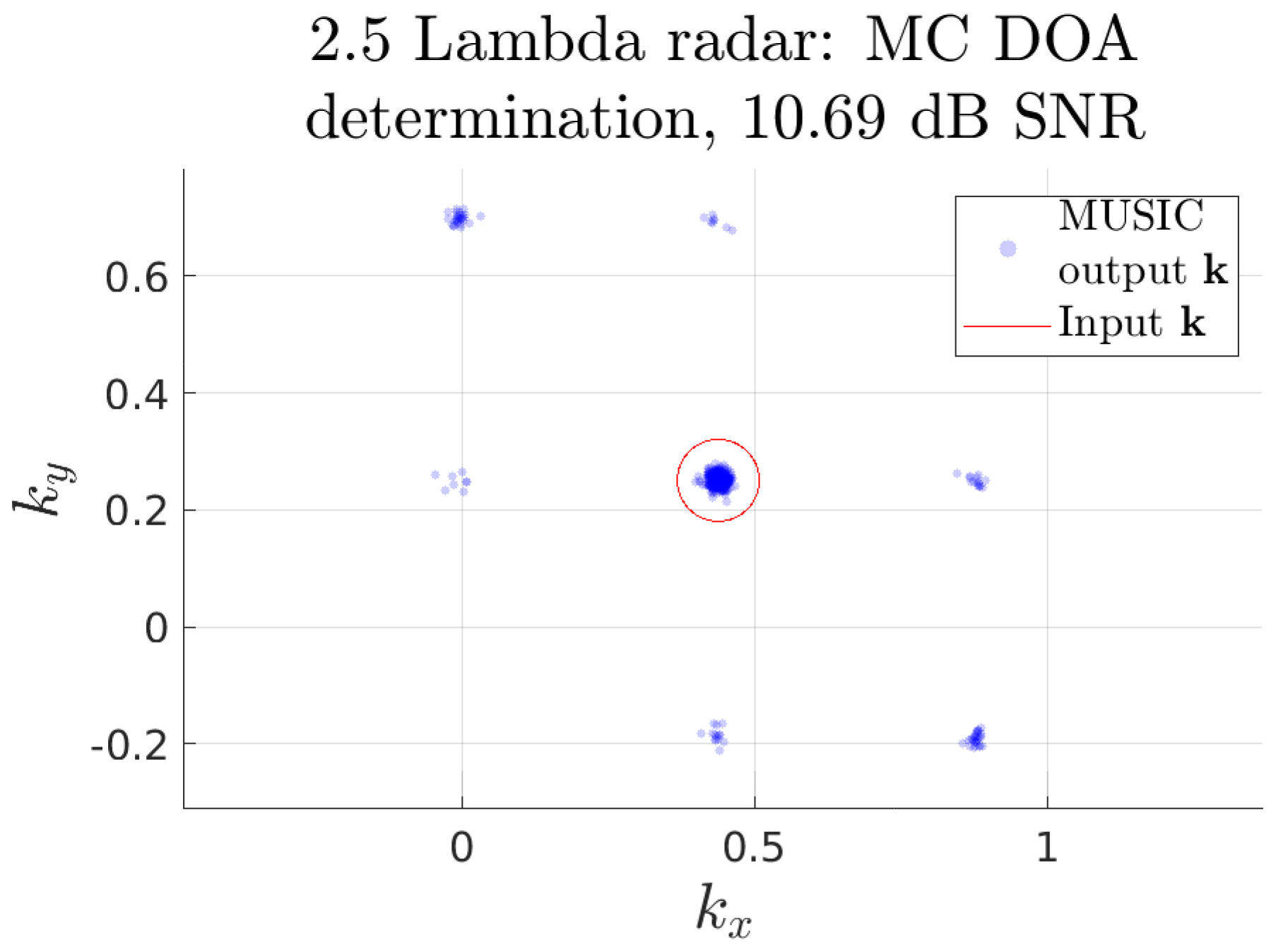
Figure 2Example Monte Carlo (MC) direction of arrival (DOA) determination simulation with 500 samples. The generic Jones 2.5λ radar model, as described by Eq. (30), was used to simulate the raw data. Noise was introduced to an equivalent signal-to-noise ratio (SNR) of 10 dB. The simulated noisy raw data were analysed using the two-step multiple signal classification (MUSIC) algorithm (Sect. 3). The input DOA was located at 0∘ azimuth and 75.5∘ elevation. At this SNR, noise-induced ambiguities are clearly visible. The probability that the output is associated with the input is 79 %.
2.5 Discretising the problem
The example MC DOA determination simulation in Fig. 2 contains apparent noise-induced ambiguities alongside the spread of the DOA estimation around the input direction and its ambiguities. This sampling of represents a continuous distribution that contains information about both the DOA determination accuracy and possible ambiguities. There are many works that describe the error distribution of MUSIC for DOA determination in radars (e.g. Kangas et al., 1994, 1996; Ferreol et al., 2006). Here, we focus on the probability of ambiguous DOA output and the general algorithm stability. Therefore, we discretise the problem by using the set of known ambiguities ki∈Ω(k0) described in Sect. 2.1.
To account for a limited DOA determination accuracy, we choose an inclusion distance s in the wave vector ground projection plane. This distance determines the region around an ambiguity and the true direction, within which we consider that particular ambiguity to be chosen by the algorithm. Thus, in the discretisation process, outputs will be considered as associated to either an ambiguity or the true DOA; otherwise, they have no association.
Practically, in the following, if:
then the sample is counted towards the probability Pi for output point ki, assuming true input k0. The samples which cannot be associated with any inclusion region are considered as algorithm failures, i.e. .
We are interested in the misclassification and algorithm failure probability. We examine this by regarding the source as a variable j and constructing a discrete conditional probability as a function of both source and output location, i.e. only the rows i sum to 1.
Even though ambiguities are not necessarily transitive relations, as mentioned in Sect. 2.1, there may still be some overlap in the inclusion regions when we define them as ki∈Ω(kj). We therefore need to give some thought to how to practically discretise the problem. If we consider the usage of the simulations as a tool for evaluating a set of ambiguous observations , then one can choose a k0 using this set of observations, by, for example, picking the mean of the largest cluster or picking the kobs−l with the largest SNR.
Assuming that we have chosen an echo from the target and that our models are representative, then either k0 or one of its ambiguities Ω(k0) is the true source. Consider that an ambiguity ki∈Ω(k0) would have an ambiguity kh∈Ω(ki) which is not part of our original set kh∉Ω(k0). The probability that kh is the source is zero as it could not have generated our observation k0.

To provide a set of input and output wave vectors that accounts for all possible true k, two separate sets of points ΩX and ΩY should be formed. The process of constructing these sets is illustrated in Fig. 3. This is useful when quantitatively evaluating measurements as the same set ΩY of output regions i can be used for all simulation inputs j from the set ΩX. The set ΩY is chosen as the collected set of all ambiguities to the simulated sources, i.e. .
Practically, considering several sets of ambiguous measurements from independent events, i.e. , were analysed using the methods proposed here. If the individual ambiguity sets Ω(kj) consistently do not explain the clusters of measured output wave vectors, there is a high probability that either the applied models are wrong or other effects are influencing the DOA determination. These effects could be radar-phase calibration issues (e.g. Chau et al., 2014), antenna malfunctions or erroneous phenomena models (e.g. multiple simultaneous signals, signal interference or wave diffraction).
There are some practical consideration when implementing the construction of ΩX and ΩY, namely that duplicate locations should not be included in ΩY. These are handled by removal based on closeness in relation to the inclusion radius. The ordering of the sets ΩX and ΩY are so that the first elements of ΩY correspond to the elements of ΩX for clarity when examining simulation results.
Using the definitions for ΩX and ΩY, we represent the probability Pij as a matrix, excluding all irrelevant association probabilities. Taking a second look at Fig. 2, one can imagine how a column of this matrix would be constructed. For each DOA in ΩY, we count the output inside its inclusion radius. The probability Pij is this number divided by the total number of samples. For the particular example in Fig. 2, the probability that the output is associated with the true input is 79 %.
The columns of the matrix Pij describe different DOA inputs for the simulation, and its rows describe the probability that the DOA determination algorithm outputs a location as the result. The most desirable form of this matrix would be a diagonal unit matrix, i.e. given true input j, the DOA algorithm always finds the corresponding location as the output. Unfortunately, this is not always the case as this probability matrix is a function of the SNR, Pij(SNR).
The error of the probability matrix Pij estimation can be determined using a Bernoulli distribution. The discretisation can be viewed as a set of Bernoulli distributions that define a success as “the output DOA fall into the inclusion region” and a failure as “it did not”. Then, we can measure the probability parameter Pij for a region and the Bernoulli distribution i, given input j through the fraction of samples inside that region out of all samples, i.e. . This estimator's variance , i.e. the accuracy of estimation, can be approximated by substituting the distribution variance with the measured Bernoulli variance and applying the central limit theorem as follows:
where Ns is the number of samples. This estimator variance has an upper limit where the parabola is maximum at . As such, the largest estimator standard error is . Using 1000 samples, the largest error in probability is %.
2.6 Bayesian inference
It is generally not advisable to use data that are ambiguous. Quantitatively describing when data are too ambiguous for further usage is one of the goals of this study. For example, as illustrated in Fig. 2, which represents a simulation of a measured event, the event could be analysed given that enough independent echoes were measured. The reason why the event is usable is that the simulation shows that the true direction has by far the highest output probability. This means that one can pick the largest cluster of output DOAs and conclude that this probably represents the true DOA. However, for more complex radar systems and other input DOAs, the situation would look different. This line of reasoning also does not give us a quantitative confidence in our choice of true DOA.
If there is a need to analyse ambiguous data, we suggest a Bayesian approach. As an example, let us return again to the simulation presented in Fig. 2. We argued that, using the simulation results when given enough independent measurements of such an event, the measurements could be used to infer the true DOA of the target. Bayesian inference generalises this type of argument by optimally using all available information to assign probabilities to all possible true input DOAs.
Given a model with parameters x that represents an event which has generated some observations D, Bayesian inference can be used to find the probability distribution of possible model parameters given the observed data, i.e. 𝒫(x|D). This distribution is called the posterior. Here | indicates conditional probability, i.e. 𝒫(A|B) is read as the probability of A given B. The posterior is calculated through the use of Bayes' theorem, as follows:
The 𝒫(x) term is called a prior probability, i.e. it describes what we think the probability distribution of possible model parameters is before any observations. One can view Eq. (18) as an update of the prior distribution by including the knowledge gained from the new observations D. The 𝒫(D|x) term describes how probable the observed data are, given the model parameters x, which is commonly called the likelihood function in the Bayesian inference community. Finally, the term 𝒫(D) can be viewed as a normalisation constant. It is commonly referred to as the prior predictive distribution as it describes the probability of the data prior to updating our belief.
This approach is compatible with the problem at hand. Assuming the matrix of probabilities Pij is calculated and known, the probability of observing ki, given the input kj, is exactly given by Pij. Therefore, in the following:
For the first observed DOA, the prior is uniform over all kj, as follows:
where NI is the number of columns in Pij, i.e. the size of ΩX. If we observe i=a1 as the first calculated DOA, we can find the posterior as follows:
If subsequent DOAs are observed, we update the probability distribution over the model parameters by setting the last posterior as our prior and applying the same formula, as follows:
If the observations ax are done at different SNRs, the Pij matrix should be allowed to change for every update x as Pij(SNRx).
This method may be able to infer the true direction even in very ambiguous data. At the very least, this method provides a probability distribution over the possible directions, as exemplified in Sect 5.
2.7 Ambiguous measurement simulation
A method for investigating whether the Bayesian approach makes a significant improvement on analysis is measurement simulation. The matrix Pij describes the probability of the DOA determination generating the output indexed i given a noisy measurement of the true input DOA indexed j. We can thus simulate measurements as a multinomial distribution, where the distribution probabilities are given by a column j of the Pij matrix. Sampling this multinomial distribution will give a set of n-simulated measurements as a list of location indices (i.e. output DOAs). Given this list of indices, Eq. (22) can be applied to calculate the most probable input, given the simulated data, without running the DOA determination algorithm. We can repeat this process to obtain a simulated distribution for the posterior 𝒫x(kj). This distribution is what we would expect to see as inference results from a measurement series of n points, given some true input. This distribution is useful for evaluating both the method itself and the radar system as it contains the probability of the Bayesian inference finding the true input. This information can thus also provide the minimum SNR and measurement number needed to achieve a desired success rate in DOA determination, assuming the Pij matrices accurately model reality.
2.8 Impact of phase offsets
Effects like mutual coupling, errors in cable lengths and other hardware-related issues can introduce phase errors in radars (Chau and Clahsen, 2019). In Appendix A, we show that phase offsets on the radar channel level do not affect ambiguity dynamics if taken into account in the DOA analysis. If phase offsets are unknown, they affect the accuracy of the DOA determination and the ambiguity dynamics.
There has been extensive work done to determine phase offsets as a whole on radar channels (e.g. Chau et al., 2014; Chau and Clahsen, 2019), but we have found no work that has empirically measured or modelled the phase offsets of individual antennas within a subgroup for the radars examined here. Therefore, we cannot simulate a realistic distribution of phase errors within subgroups.
To examine the impact of phase errors on the antenna level within subgroups, we performed a pair of MC simulations for the MU radar subgroup model. As input, the ΩX set for kI, as given in Sect. 5, was used. For each antenna, a random phase error between −45 and 45∘ was introduced. Then, an MC simulation at an SNR of 3 dB was performed for both the phase error model and the standard model. The probability matrix for each of these simulations was calculated, and the difference between them was examined. There was practically no difference in the probability matrices.
It should be noted that in this test the phase offsets that generated the simulated noisy signal were also included in the MUSIC analysis model. Finally, we ran two MC simulations at 5 dB SNR for the MU subgroup model, using kI and kII as input DOAs. In these simulations, the noisy signal was generated with channel phase offsets measured using a technique similar to the one presented in Chau and Clahsen (2019) but analysed using no phase offsets. For these two cases, the uncorrected phase offsets did not impact the ambiguity dynamics, but it did introduce a small error in the DOA determination accuracy. As such, the results presented here are applicable in general when phase errors are measured or modelled and possibly even when not measured or modelled. Further examination of the impact on ambiguities of unknown phase errors is desirable but outside the scope of the current study.
For the purposes of consistency and simplicity, we have used the same DOA determination method for all radar systems examined, namely the MUSIC algorithm (Schmidt, 1986). This method allows for an arbitrary sensor response model Φ and can thus be applied on all systems. MUSIC is practically equivalent to beam-forming DOA methods but with reduced variance due to the subspace approach. We here give a short overview of how we have applied the MUSIC method.
We define a measured sensor response as the complex vector x∈ℂN. The sensor response model in Eq. (1) refers to a so-called decoded signal. The decoded signal is the signal coherently integrated over all temporal samples of a radar pulse. However, the lowest level of raw data also contains these temporal samples of the radar pulse. Given M temporal samples of the coded pulse, the measurement matrix then consists of N rows and M columns as follows:
The correlation matrix R of our measurements is calculated using matrix algebra as follows:
The correlation matrix consists of coherently integrated channel-to-channel phase differences over the temporal samples. The eigenvalues of the correlation matrix correspond to signal powers, and the eigenvectors corresponding to the largest eigenvalues span the signal subspace (Schmidt, 1986). If there is noise, the eigenspace spans the entire sensor configuration space, otherwise it only spans the signal subspace. First, we extract the eigenvectors Pi and eigenvalues λi of the correlation matrix using standard linear algebra methods. Then, assuming one signal subspace dimension, i.e. one signal from one direction, we define the noise subspace as the column space of the following:
where Pj corresponds to the largest eigenvalue . This eigenvector represents the signal subspace. MUSIC is a multiple signal classification method. If there are multiple signals present in the data, the second eigenvector and eigenvalue is associated with the second strongest signal, etc. As the column vectors of Q form an orthonormal basis, we consider the space as follows:
The scalar projection function P into this linear subspace ℚ is as follows:
The space ℚ represents the noise; thus, any space orthogonal to ℚ is a signal. The projection of a vector onto an orthogonal space is zero; thus, we are searching for vectors x that minimises Pℚ(x).
We write the projection function in terms of matrix operations as follows:
Normalising and inverting the projection, we maximise instead of minimise and find the familiar MUSIC function. As we have a model for x as a function of DOA, we set x=Φ(k) and find the following:
which is the form usually recited in literature. This function needs to be maximised by an appropriate method to find the sensor response Φ(k) that best matches the detected signal, thereby also determining the DOA, k, of the signal.
As Eq. (29) takes the scalar projection onto the signal complement space, the function is invariant to the orientation of the vector with respect to the signal subspace basis. Thus, the definition in Eq. (6) is appropriate for describing the ambiguities of MUSIC.
We have chosen to apply a two-step maximisation method. First, a finite grid search over all possible k was applied. Then, the maximum found during this grid search was used as an initial condition for a gradient ascent applied on ∇f(k) to find the peak point. Finally, the peak value is used as output, i.e. as the determined DOA of the signal.
However, there is no guarantee that the initial grid search will always be able to identify the correct slope as an initial condition for the gradient ascent. If the peak width is smaller, then the grid size of any slope may be found instead. To solve this problem, we also implemented an option of running multiple gradient ascents in parallel. When this option is enabled, instead of using only the maximum point from the grid search as a starting value, the N largest values that are separated from each other by at least δX in kx,ky space are used. The separation condition ensures that no two starting points are located on the same slope. These N starting points are explored by a gradient ascent, and the largest peak among them is chosen as the algorithm output.
The sensor response for all radars covered in this study was modelled using two different models, with a simplified model as follows:
where ni is the number of antennas summed to that radar channel. And a model using the subgroup gain patterns was implemented as follows:
The exceptions are the Jones-type radar systems in which there are no subgroups but only single antennas. As previously mentioned, in these models ri indicates the locations of individual antennas or the geometric centres of the sub-arrays, i.e. the phase centres.
In this study, we have assumed that the antennas have omnidirectional gain. This is, of course, not the case as mentioned in Sect. 2, but this assumption has no impact on the current study. As all radar systems examined have the same antennas throughout the system; the individual gain function for an antenna cancels in any algorithm that is invariant to signal amplitude. However, in the implementation of a data analysis pipeline, it is important to implement the individual antenna gain pattern γ and the subgroup generated gain patterns in the sensor response model to be able to determine the radar cross section correctly.
We hereafter refer to the model in Eq. (30) as the phase centre model and the model in Eq. (31) as the subgroup model.
In Fig. 4, the antenna positions of all examined radars are illustrated so that their individual configurations and sizes can be compared.
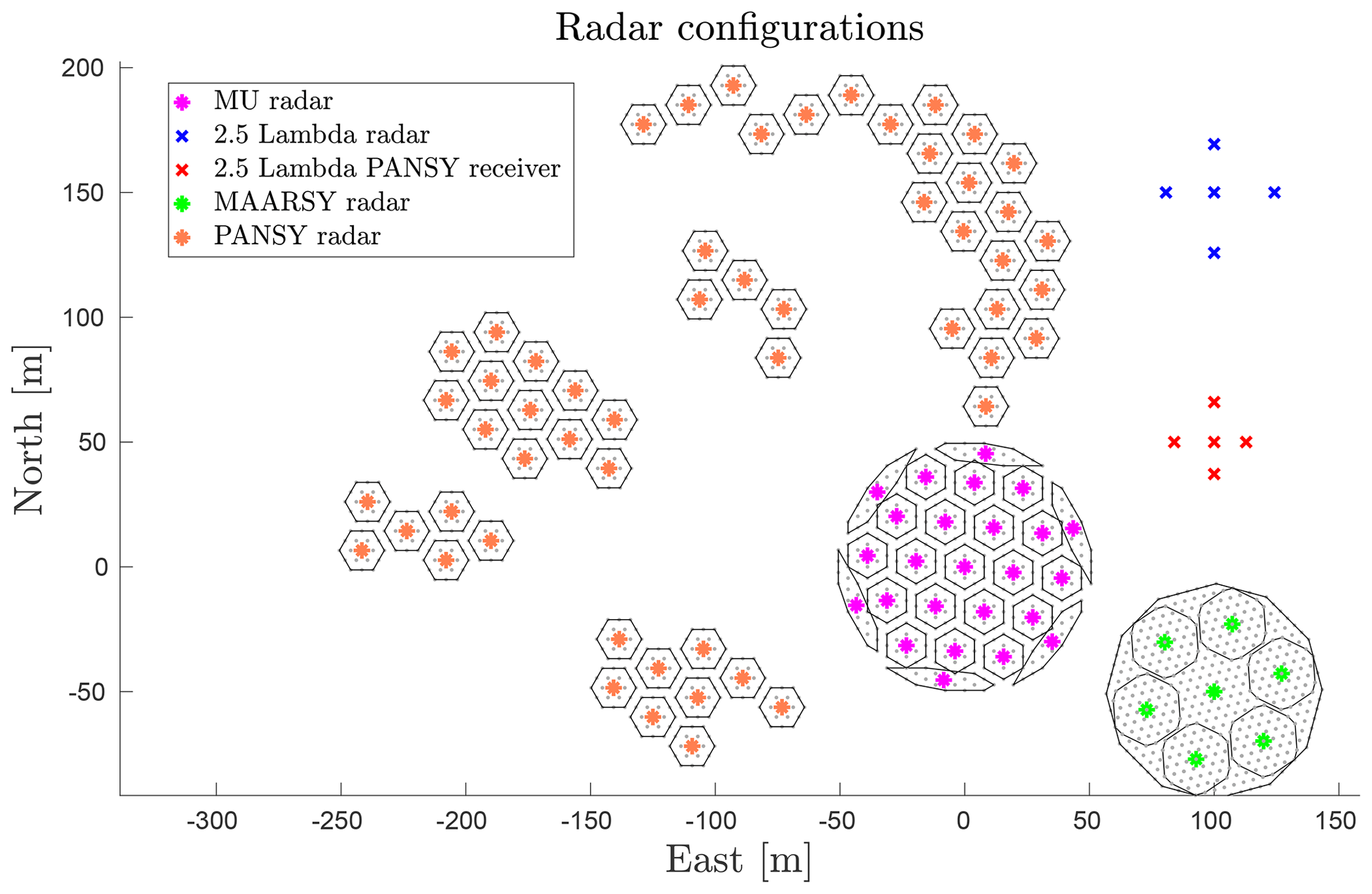
Figure 4The different radars considered in the DOA determination study. For the radars which consist of subgroups of antennas, the subgroup centres have radar-specific colours, while antennas and subgroup borders are always grey and black. The Jones 2.5λ radars are single-antenna channel radars; thus, coloured markers indicate antennas here.
4.1 Jones 2.5λ radar
Radar systems designed for studying meteor trail echoes commonly consist of a wide angle (all-sky) transmitter system and an interferometric receiver system (e.g. Jones et al., 1998; Hocking et al., 2001).
The receiver system design is beset by two problems (Jones et al., 1998), namely that antennas spaced more than λ∕2 apart give rise to ambiguities in the DOA, and that antennas spaced less than λ∕2 apart give rise to strong mutual impedance. The so-called Jones 2.5λ radar configuration is an elegant solution suggested by Jones et al. (1998) to remedy the situation. The solution consists of using five antennas, with one central antenna and two spaced by 2.5λ and 2.0λ in each of the two perpendicular cardinal directions (see Fig. 4).
As described by Jones et al. (1998), the phase measurements at the outer antennas relative to the central antenna can ideally be used to calculate an unambiguous determination of the echo DOA, taking advantage of the fact that the internal antenna distances to the central antenna differ by λ∕2. Furthermore, the phase difference of antennas with 4.5λ spacing is used to give better angular precision at the cost of ambiguous DOA, the most probable solution of which is then selected using the λ∕2 phase difference.
Holdsworth (2005) investigated the Jones antenna configuration and found that the usage of 2.5, 3 and 5.5λ spacings could produce more accurate echo DOA. Younger and Reid (2017) developed the concept further and presented a solution which utilises all possible antenna pairs of a meteor radar antenna configuration, similar to the DOA calculations using MUSIC in this paper. In addition to providing results in excellent agreement with the original interferometric algorithm by Jones et al. (1998), the method presented by Younger and Reid (2017) and the MUSIC algorithm allow for different layouts.
The Jones antenna configuration has remained predominant in meteor radar installations and is often referred to as removing (in principle) any angular ambiguities (Hocking et al., 2001). However, as was pointed out already by Jones et al. (1998), the determination is sensitive to noise and only unambiguous if the SNR is large enough. The original simulations by Jones et al. (1998) showed that the method started to produce incorrect apparent echo directions for elevations greater than 30∘ when the SNR was below 17 dB, but that, at the same time, the fraction of these was small down to about 10 dB. The standardised All-Sky Interferometric Meteor Radar (SKiYMET) software meteor-detection data contain an ambiguity level classification. If the ambiguity parameter is equal to 1, the data were determined to be unambiguous, and if it is greater than 1, then there is a possibility that the meteor was erroneously located (Hocking et al., 2001).
To our knowledge, there are no further quantitative investigations of the Jones 2.5λ radar configuration performance, except for the studies mentioned above and references therein. The results of applying the method presented in this paper on the Jones 2.5λ radar to quantify noise-induced ambiguities are given in Sect. 5.1. As the mentioned previously, studies on ambiguities already exist; thus, simulating a Jones 2.5λ radar also provides a good reference simulation for validation of the methods presented in Sect. 2.
4.2 MU radar
The 46.5 MHz Middle And Upper Atmosphere (MU) radar near Shigaraki, Japan (34.85∘ N, 136.10∘ E), has a nominal peak transmitter power of 1 MW and a maximum beam duty cycle of 5 %. The present setup of the MU radar hardware comprises a 25 channel digital receiver system. It was upgraded from the original setup (Fukao et al., 1985) in 2004 and is described by Hassenpflug et al. (2008). After the upgrade, the MU radar always transmit right-handed circular polarisation and receive left-handed circular polarisation, with a phase accuracy of 2∘. The output of each digital channel is the sum of the received radio signal from a subgroup of 19 Yagi antennas. The whole array consists of 475 antennas, evenly distributed in a 103 m circular aperture, with a main lobe maximum gain of 34 dB and a minimum half-power beam width of 3.6∘. A schematic view of the array and the subgroups is given in Fig. 4.
Early meteor head echo measurements, using the original setup with four receiver channels (Nishimura et al., 2001), are not investigated further in this study. The focus is instead on the current 25 channel set-up, which has been used more extensively for hard targets such as meteors (e.g. Kero et al., 2011, 2012a, b, 2013; Fujiwara et al., 2016; Kastinen and Kero, 2017).
4.3 MAARSY radar
The new Middle Atmosphere Alomar Radar System (MAARSY) was constructed in 2009–2010 on the Norwegian island of Andøya (69.30∘ N, 16.04∘ E), following similar design principles as for the MU radar. It is a monostatic radar operated at 53.5 MHz, with an active phased array antenna consisting of 433 Yagi antennas (Latteck et al., 2010). The antennas are, similar to the MU radar, arranged in an equilateral triangle grid with 0.7λ (4 m) spacing, forming a 90 m circular aperture. This results in a rather symmetric radar beam, with a maximum directive gain of 33.5 dB and a minimum half-power beam width of 3.6∘. Each individual antenna is connected to a transceiver with independent phase control and output power up to 2 kW, enabling flexible beam forming, beam steering and approximately 800 kW peak transmitter power with 5 % duty cycle.
The smallest MAARSY sub-array unit consists of seven antennas distributed in a hexagonal pattern, as illustrated in Fig. 5. The receiver system currently allows for 16 separate channels. Early meteor head echo observations with MAARSY used eight channels which were defined according to Fig. 4, where seven of the channels consisted of the combined input from seven sub-arrays (i.e. 49 antennas) and the eighth channel contained the combined input from all antennas (Schult et al., 2013). Later meteor head echo observations have made use of the alternative MAARSY configuration shown in Fig. 5 (Schult et al., 2017).
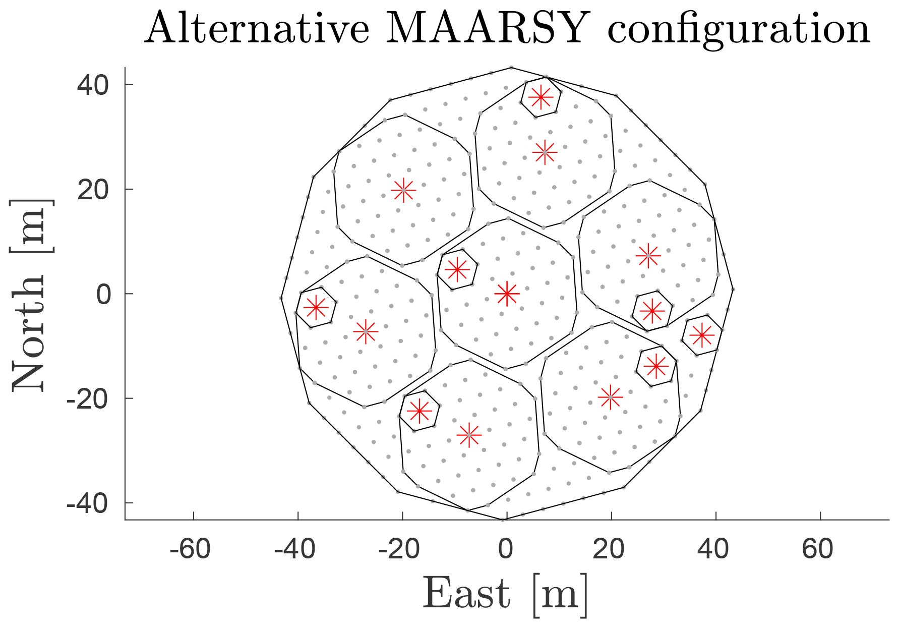
Figure 5An alternative configuration of MAARSY subgroups used as radar channels to the one illustrated in Fig. 4. In this configuration, 15 channels are used instead of eight so as to include the information from smaller but closely located hexagonal groups, thus producing shorter baselines for less ambiguous interferometry (Schult et al., 2017).
The radiation pattern of MAARSY has been studied and validated through observations of cosmic radio sources (Renkwitz et al., 2012, 2013), scattering of a sounding rocket's payload (Renkwitz et al., 2015) and meteor head echoes (Renkwitz et al., 2017). Methods have also been developed to calibrate and validate the measured phases of the individual channels, using cosmic radio noise and meteor head echoes (Chau et al., 2014).
4.4 PANSY radar
The Antarctic Syowa Mesosphere Stratosphere Troposphere Incoherent Scatter (PANSY) is a mesosphere–stratosphere–troposphere/incoherent scatter (MST/IS) radar located at the Japanese Syowa Station (69.01∘ S, 39.59∘ E) in the Antarctic (Sato et al., 2014). The first sub-arrays of the PANSY radar were installed in 2011. The first continuous observations of polar mesospheric summer echoes were made with a single sub-array in January–February 2012. Due to snow accumulation in the originally symmetric antenna field consisting of 1045 crossed Yagi antennas summed into 55 channels, several of the sub-arrays were moved to higher ground, as illustrated in Fig. 4. This is the antenna configuration we have used in the simulations.
PANSY operates on a centre frequency of 47 MHz and with a peak power of 500 kW and 5 % duty cycle. The radar is a challenge for DOA determinations as the subgroups are located at different altitudes and partially disjointed and have to be moved or intermittently be disconnected from the system, depending on snow accumulation conditions. Even the antennas within subgroups are elevated non-symmetrically. Currently the antennas are distributed in altitudes ranging between −2 and +8 m from the reference plane.
In 2017, a peripheral antenna array for detecting field-aligned irregularities (FAI) was installed (Hashimoto et al., 2019). This has enabled the suppression of FAI echoes and increased the number of power profiles usable for incoherent scatter measurements of the polar ionosphere by more than 20 %. In this paper, we do not investigate the peripheral FAI array.
4.5 PANSY meteor radar
The PANSY radar has recently been complemented by a meteor trail echo interferometric receiver system (Taishi Hashimoto, personal communication, 2020). The antenna configuration is displayed in Fig. 4. Since the operating frequency of PANSY (47 MHz) differs from meteor radar systems (typically 35 MHz), the configuration is more compact when displayed in units of metres, even though the number of wavelengths are the same. The main difference between the PANSY meteor radar receiver and the Jones 2.5λ radar is that the former is not a planar array but that the antennas are displaced in the vertical (z) direction with up to 0.8 m, corresponding to ∼0.12λ.
To demonstrate the above methods, we present results from numerical simulations. The next step will be applying them on measurement data. We aim to implement these methods in our data analysis pipelines for meteor head echoes measured by the MU radar and the PANSY radar in the future and to classify the location probability of ambiguous meteor radar trail echoes using Bayesian inference. However, the current study allows us to quantitatively evaluate how DOA determination behaves with respect to SNR and to qualitatively evaluate if ambiguities are relevant or not. Such results are useful in the configuration and construction of pipelines.
For each of the radar systems described in Sect. 4, we have applied the methods described in Sects. 2 and 3. Three input directions k0 were chosen as sources:
- I.
kI= azimuth: 0∘, elevation 75.5∘,
- II.
kII= azimuth: 0∘, elevation 90∘,
- III.
kIII= azimuth: 45∘, elevation 40∘.
For each of these chosen sources, the following steps were performed:
-
Determine all ambiguities using 1000 starting conditions according to the method outlined in Sect. 2.1. This generates the ΩX and ΩY sets.
-
Run an MC simulation of 500 samples for each input direction in ΩX at all SNR levels, according to the method outlined in Sect. 2.4. An appropriate range of linearly spaced SNRs in decibel was used to capture the transition from stable DOA determination to complete algorithm failure.
-
Discretise the MC results into probability matrices Pij, using the sets ΩX and ΩY according to Sect. 2.5 with an inclusion radius of s=0.07.
-
Simulate measurements according to Sect. 2.7, and calculate Bayesian inference distributions according to Sect. 2.6, if applicable.
The ambiguity dynamics change as a function of input DOA for all systems but the planar Jones 2.5λ configuration. A complete overview of the indicator function d(k,k0) is therefore 4D. To visualise the ambiguity dynamics, a grid of k vectors over all possible k0 was used, and only the worst ambiguity was saved for each grid point. That is, on each grid point, k0 all ambiguities were calculated, and the maximum value ambiguity was saved for that direction.
This kind of map shows in which source directions the radar is able to resolve well and in which directions it cannot uniquely determine. While it does not illustrate the morphology of ambiguities, it does show the qualitative connection between input DOA and limiting SNR. The white areas are regions where no ambiguities were found using the selected algorithm settings.
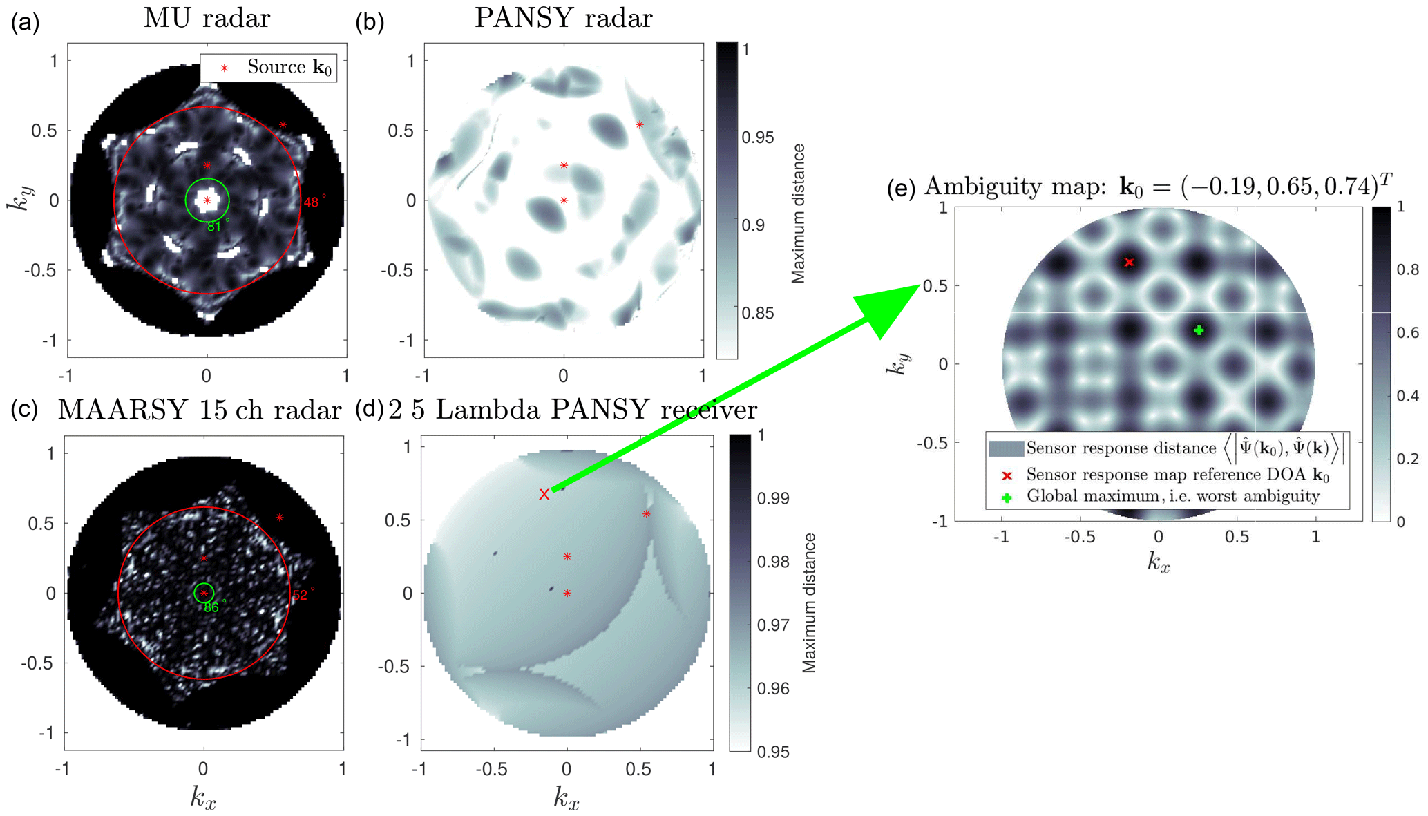
Figure 6Map of worst ambiguity as a function of input DOA for the MU radar subgroup model (a), the PANSY subgroup model (b), the MAARSY 15 channel radar subgroup model (c) and the 2.5λ receiver model (d). For each k0, an ambiguity search over k of d(k,k0), as defined in Eq. (6), was performed. The result from the ambiguity search yields Ω(k0). The ambiguity with the largest inner product to k0 gives the d value at the location k0 in the maps to the left. Using the applied colour scale, white indicates a better situation and black indicates a worse situation with respect to ambiguities. An example of such an ambiguity search result is shown in panel (e) for a particular k0. Overlaid on these maps are red crosses illustrating the further examined source directions and concentric elevation limits described in Sect. 5. Note the difference in the colour scale between the top and bottom rows.
The analysis results for each of the radar systems (except the planar Jones 2.5λ radar) are illustrated in Fig. 6. Overlaid on these maps are red crosses illustrating the chosen source directions further examined. These input DOAs kI–kIII were chosen to cover a wide range of the worst ambiguity and elevation angle. The same three directions were selected for all systems to enable cross comparisons. We did not take population models or detection probabilities into consideration when choosing these input directions.
Additionally, on the maps for the MU radar and the MAARSY 15 channel radar, two elevation limits are shown as two concentric circles. The inner circle represents the elevation above which DOA determination is practically unambiguous. The outer circle illustrates the elevation below which unambiguous DOA determination is practically impossible.
Before application on measurement data, one should validate that the sets ΩX and ΩY are predicting the behaviour of the MC simulations so that unexpected dynamics introduced by the DOA determination algorithm itself are not disregarded. If the measurement data cannot be explained by MC simulation, either the sensor response model or the phenomenon model are most likely not representative.
5.1 Jones 2.5λ radar
First, we report results for the Jones 2.5λ radar as this is the simplest system examined in the study. Furthermore, trivial and previously published results exist for reference (e.g. Jones et al., 1998; Chau and Clahsen, 2019).
Following the steps outlined above, the resulting DOA sets ΩX and ΩY for kI,kII and kIII were determined. As expected, the generated ambiguity maps indicate that the Jones configurations has prominent ambiguities at ±0.43 in the directional cosine along both of the array axes. As this is a simple radar system, these ambiguities can be found with conventional methods equivalent to the Nyquist–Shannon sampling theorem (Jones et al., 1998). These ambiguities can also be found by analytically solving Eq. (B1) from Appendix B. Any ambiguity map for the Jones system is simply a translation in k space of the map at zenith, as shown in Appendix B.
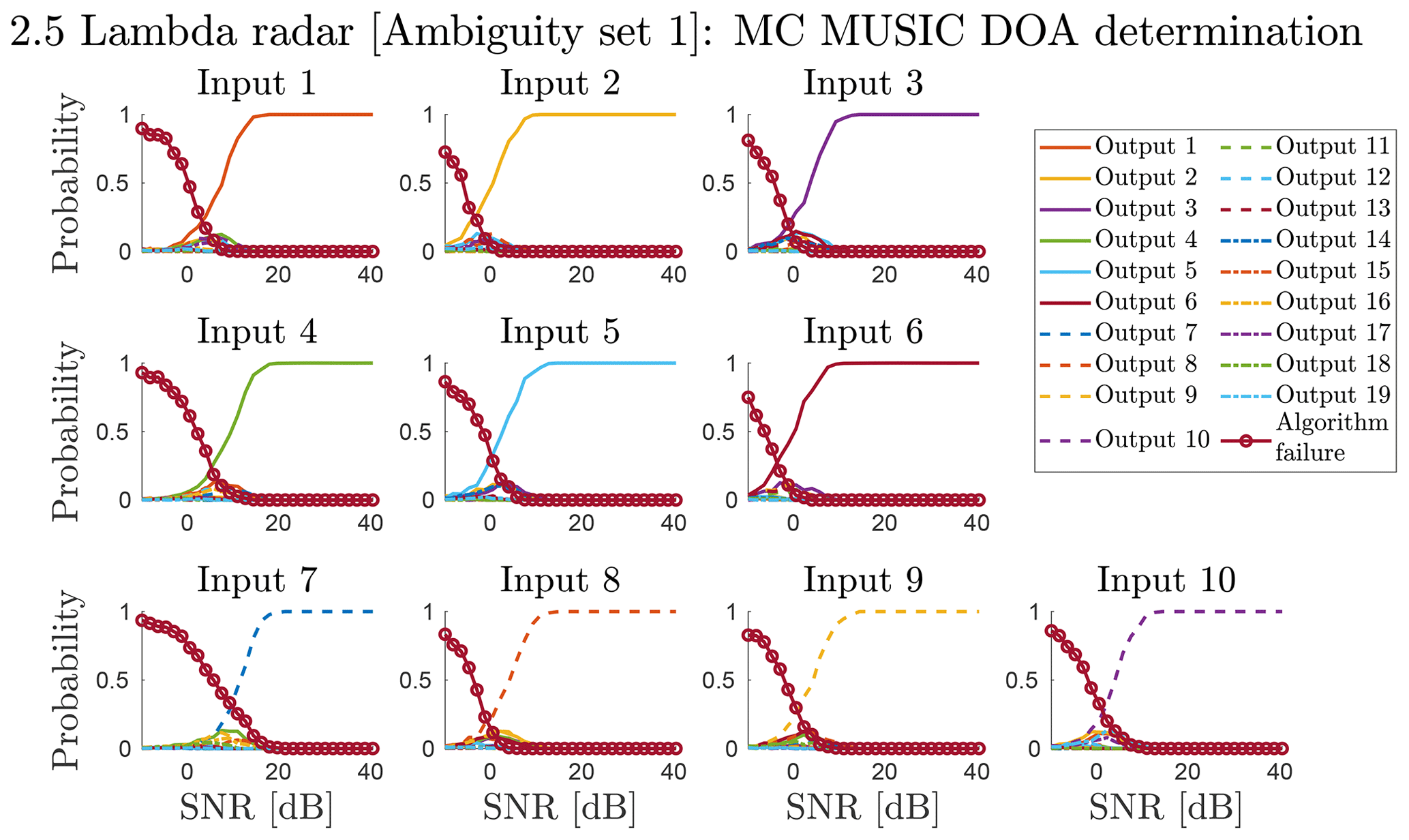
Figure 7The discretised output DOA distribution as a function of SNR and input DOA for the Jones 2.5λ radar, when using kI to generate ΩX and ΩY. Outputs 1–10 (⊂ΩY) correspond to inputs 1–10 (ΩX), while outputs 11–19 (⊂ΩY) are scattered according to the second-degree ambiguities. Numerical values of inputs 1–10 are given in Table 1 (Jones 2.5λ; I. 1–10). The DOA outputs that do not fall into any discretisation region are classified as algorithm failure.
Table 1Summary results for all input DOAs used to perform an MC DOA determination simulation. These are the ΩX sets for kI, kII and kIII. These limits show when the DOA determination with MUSIC for the respective radar system is stable to a level of 99 % output probability of the true input. Thus, for the given DOA, echoes below the given SNR are possibly ambiguous. Note: Az – azimuth angle; El – elevation angle in local radar coordinates. SNR – signal-to-noise ratio. An empty SNR indicates that none of the simulations produced an input–output correspondence of 99 % or higher. For MU, MAARSY and PANSY radars, these results are from using the model described by Eq. (31). For the Jones 2.5λ and the PANSY 2.5λ, the model in Eq. (30) was used. The indices correspond to the initial k vector and the input–output maps illustrated for each radar system in Sect. 5.
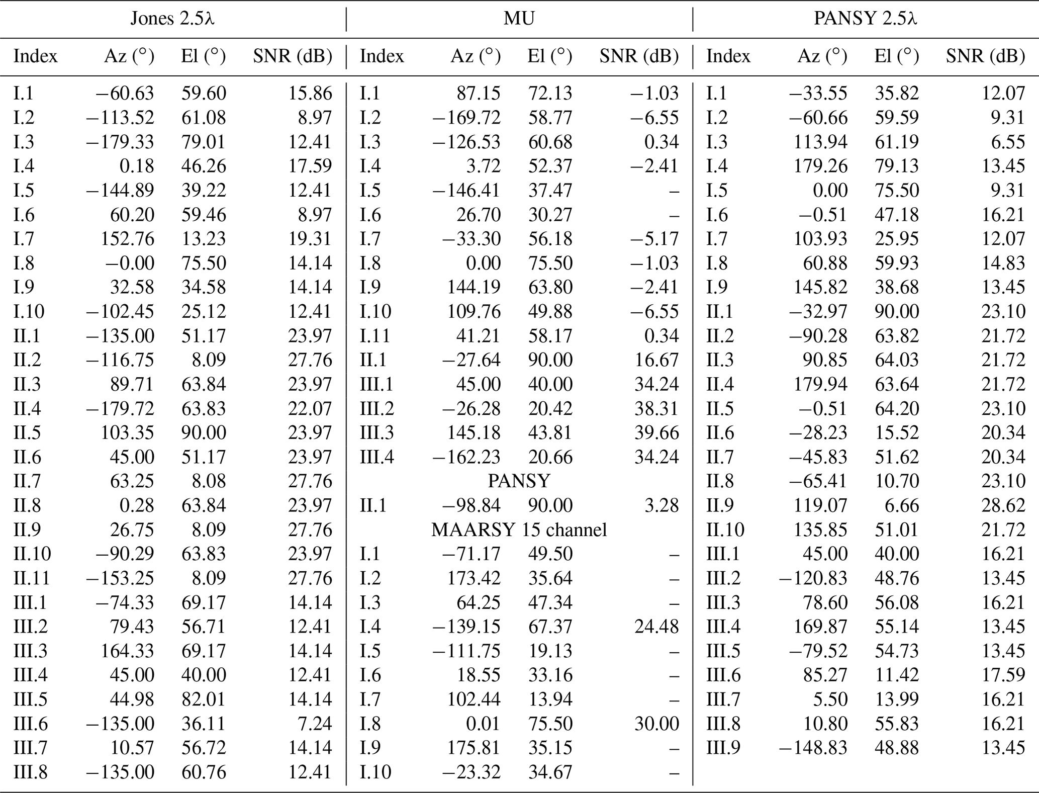
A series of MC simulations were performed using the set ΩX as input DOAs. The probability Pij was calculated for each simulated SNR using the set ΩY. The Pij matrix elements as a function of SNR are illustrated in Fig. 7 for the source kI. One panel in Fig. 7 illustrates a column of the Pij matrix, and each curve represents a row of the matrix. Output 1–10 (⊂ΩY) correspond to input 1–10 (ΩX), while output 11–19 (⊂ΩY) are scattered according to the second degree ambiguities. Numerical values of input 1–10 are given in Table 1, Jones 2.5λ and I.1–10.
As expected, the results for kII and kIII (not shown here) are practically identical (as the ambiguity maps are identical) to the ones illustrated in Fig. 7 but shifted in SNR space. The relative SNR shifts are due to array gain differences and are given numerically in Table 1.
Figure 7 shows the region where noise-induced ambiguities are relevant. For example, the DOA of input 1 is always correctly determined above 10 dB SNR. Noise-induced ambiguous solutions appear between −10 and 10 dB SNR. At lower SNR, the algorithm returns approximately uniformly distributed results classified as algorithm failure. Different input directions have different thresholds, as shown in Table 1. For most directions 10 dB array SNR is not sufficient for 99 % confidence.
Following the method outlined in Sect. 2.6, we have generated a simulated series of observations for the Jones 2.5λ radar and analysed that series with Bayesian inference to find 𝒫x(kj). We have examined how often the Bayesian inference 𝒫x(kj) was able to correctly identify the true input by assigning it the largest probability. This gives an estimation for the ideal expected success of applying Bayesian inference on ambiguous echoes for that SNR. Repeating the process for every SNR level that was simulated, we found the probability of correct classification as a function of SNR and number of observed outputs. Generally, the simulations showed that the ideal relation between needed SNR and needed observations followed an inverse relation with the number of observations.
5.2 MU radar
In contrast to the Jones 2.5λ radar, the MU radar channels consists of subgroups of antennas. If all subgroups were identical and had a reflection symmetry line, this would mathematically assure that the sub-array gains do not have imaginary components and have the same dependence on input DOA. Practically, it would mean that the sub-array gain patterns gj could be omitted. However, as is illustrated in Fig. 4, the MU radar has six outer subgroups that are not symmetrical nor equal. Thus, the subgroup gain will affect the normalised sensor response model and the DOA determination capabilities. Therefore, we consider both of the models described in Eqs. (30) and (31).
Given the MU asymmetric subgroups, one could consider the model in Eq. (30) as being unphysical. Nevertheless, the phase centre model has been successfully used to analyse meteor head echoes from the MU radar (Kero et al., 2012b). The reason is that the two models obviously converge towards the zenith and are very similar in the main lobe and first side lobes as they are both models of planar arrays. Since most meteor head echo detections occur in the main lobe of the radar, only a small portion of the events are affected by the difference between the two models.
As the ambiguity results for the phase centre model are close to trivial (see Appendix B), we do not present any ambiguity maps for that model. It is sufficient to note that there are no ambiguities with d=1 due to the geometric centres of the six outer groups breaking the symmetry of the 19 hexagonally symmetric inner groups.
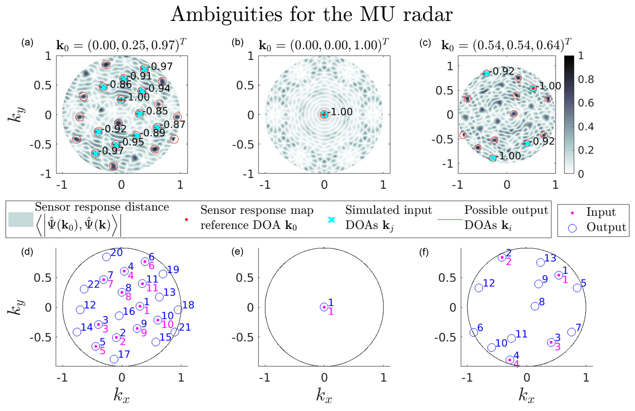
Figure 8Ambiguity analysis summary illustration for the MU radar using the subgroup model. The three columns represent the source DOAs kI (a, d), kII (b, e) and kIII (c, f). For each column, the top row consists of sensor response inner product d(k) maps calculated using Eq. (6). The value of d(k) ranges from 0 to 1 as Eq. (6) effectively describes the norm of the projection of one point on a unit sphere onto another; thus, the maximum distance is 1. Overlaid on the map is the reference DOA k0, the simulated input DOA set kj∈ΩX and the possible output DOA set ki∈ΩY. Panels (d)–(f) show an indexing map for input–output locations.
The MU radar subgroup model is expected to have an ambiguity map that varies as a function of input DOA. We present maps for kI, kII and kIII and the resulting DOA sets ΩX and ΩY in Fig. 8 to exemplify the variability in the ambiguity map morphology in addition to the variability in the worst ambiguity (see Fig. 6).
Comparing the phase centre model with the subgroup model, the DOA determination situation improves slightly for kI and kII, as many ambiguities become less prevalent. This can be attributed to the fact that the two models diverge at lower elevations, thereby making it easier to distinguish a low-elevation DOA from a DOA near the zenith. For kI, the closest ambiguities basically remain at the same distance d=0.97. Furthermore, for kIII, there is even a close-to-perfect ambiguity (d=0.999988), as illustrated by Fig. 8c. This may appear surprising as previously there were no perfect ambiguities. However, the change makes sense given the internal antenna configuration of the outer subgroups that differentiate between the ambiguities formed by the 19 inner subgroups.
The phase output of subgroup 1, the outer subgroup to the west in Fig. 4, using the subgroup model versus the phase centre model is illustrated in Fig. 9. The two red crosses correspond to the two directions labelled d=1.00 in Fig. 8c. Here it is clearly seen that the phases have equal values for these two directions when including subgroup gain in the left panel of Fig. 9, while the phase values were very different when using the phase centre approximation shown to the right of Fig. 9. This channel is the main contributor to differentiating between these two ambiguities that appear due to the 19 inner subgroups. This highlights the advantage of numerically investigating ambiguities, either by sensor response model ambiguity indicator maps or by MC simulation, as this ambiguous DOA would probably have gone unnoticed otherwise.
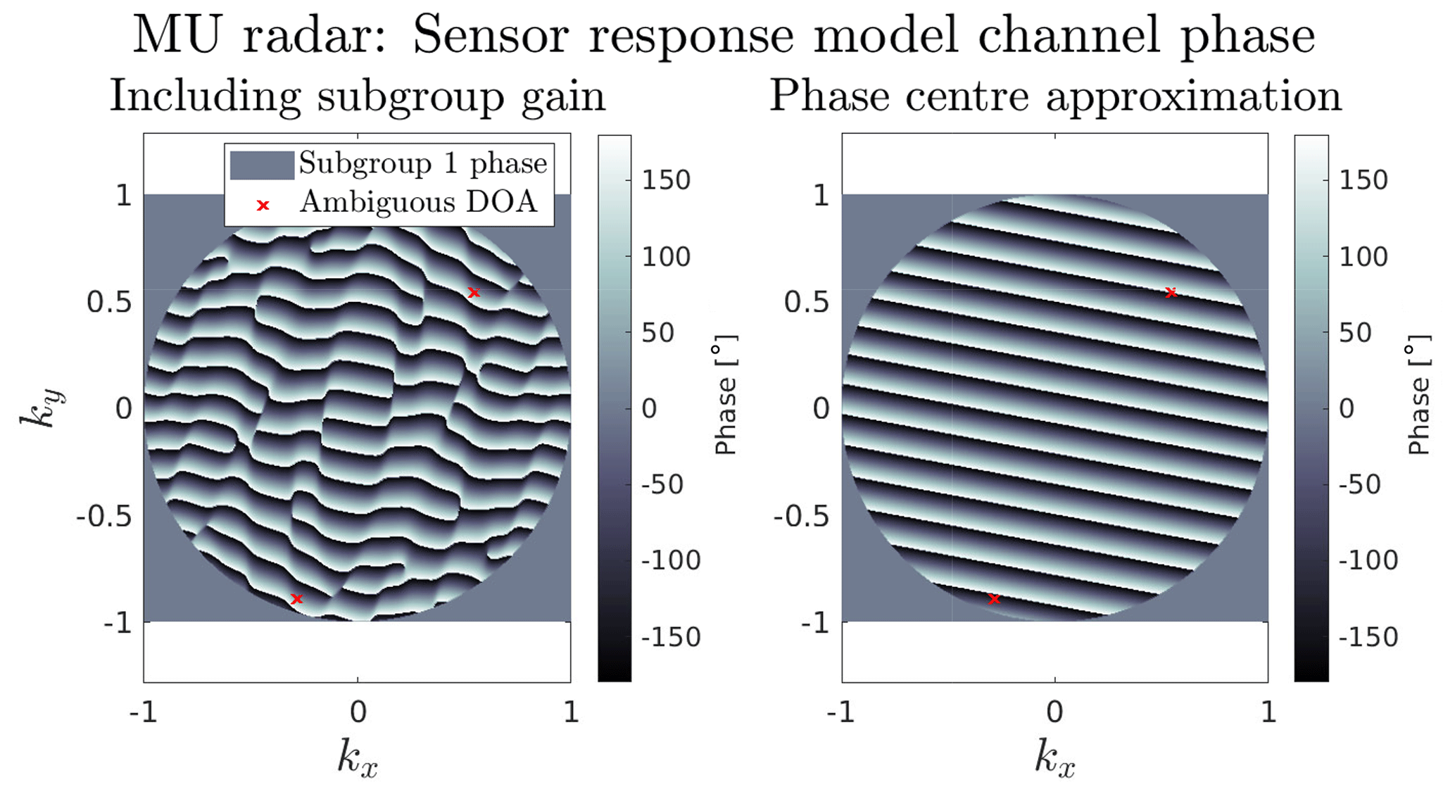
Figure 9Comparison of the signal phase measured using the subgroup model and the phase centre model of MU radar channel 1 (the outer asymmetric subgroup to the west, illustrated in Fig. 4). The inclusion of the asymmetric antenna positions in the subgroup model affects the expected phase measurements of the signal as a function of wave DOA. The two red crosses mark two directions that are ambiguous in the subgroup model but not in the phase centre model.
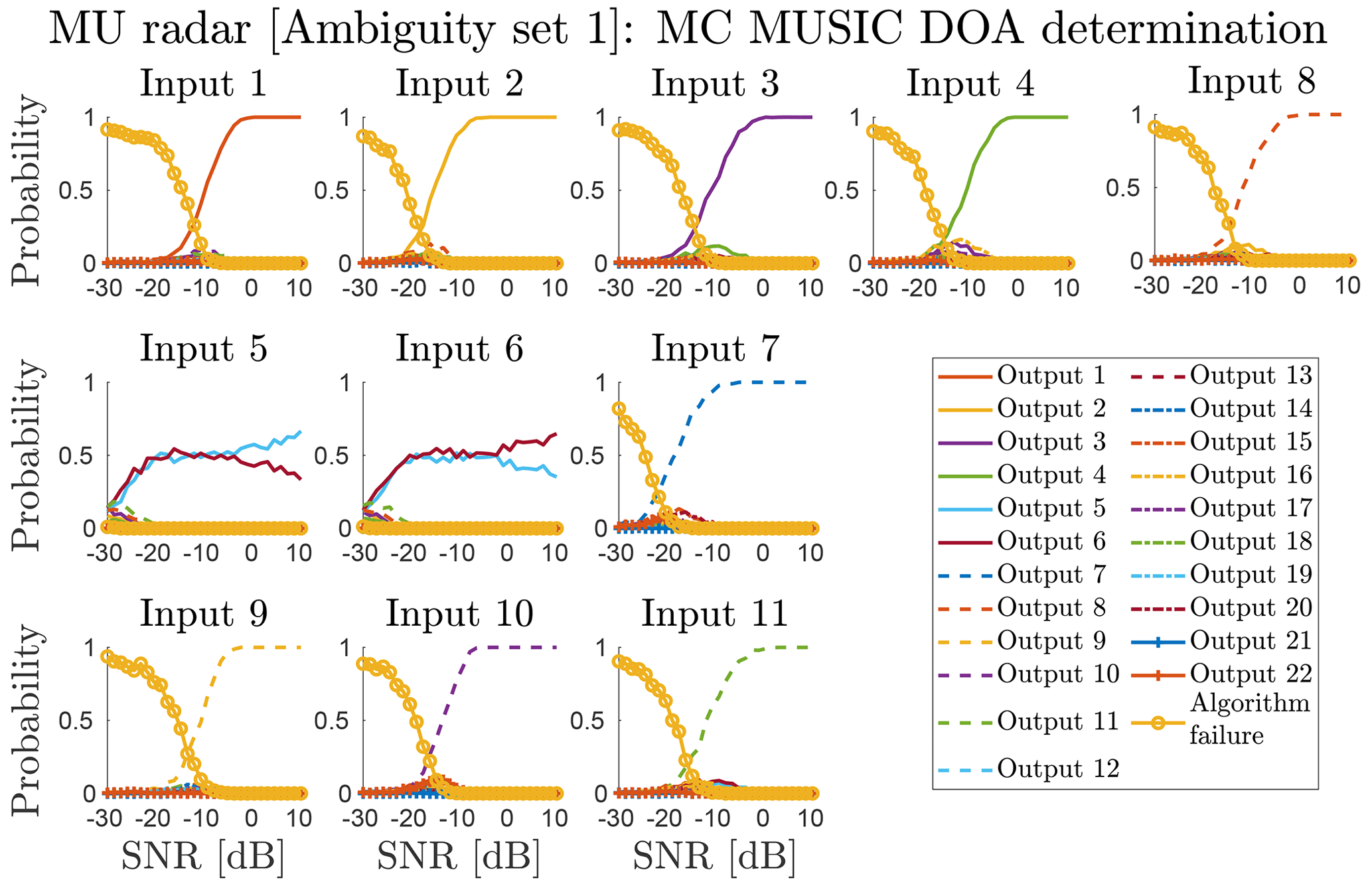
Figure 10The discretised output DOA distribution as a function of SNR and input DOA for the MU radar, using the subgroup model and kI to generate ΩX and ΩY. The numerical values of inputs 1–11 (ΩX and corresponding to output 1–11) are given in Table 1, MU; I. 1–11.
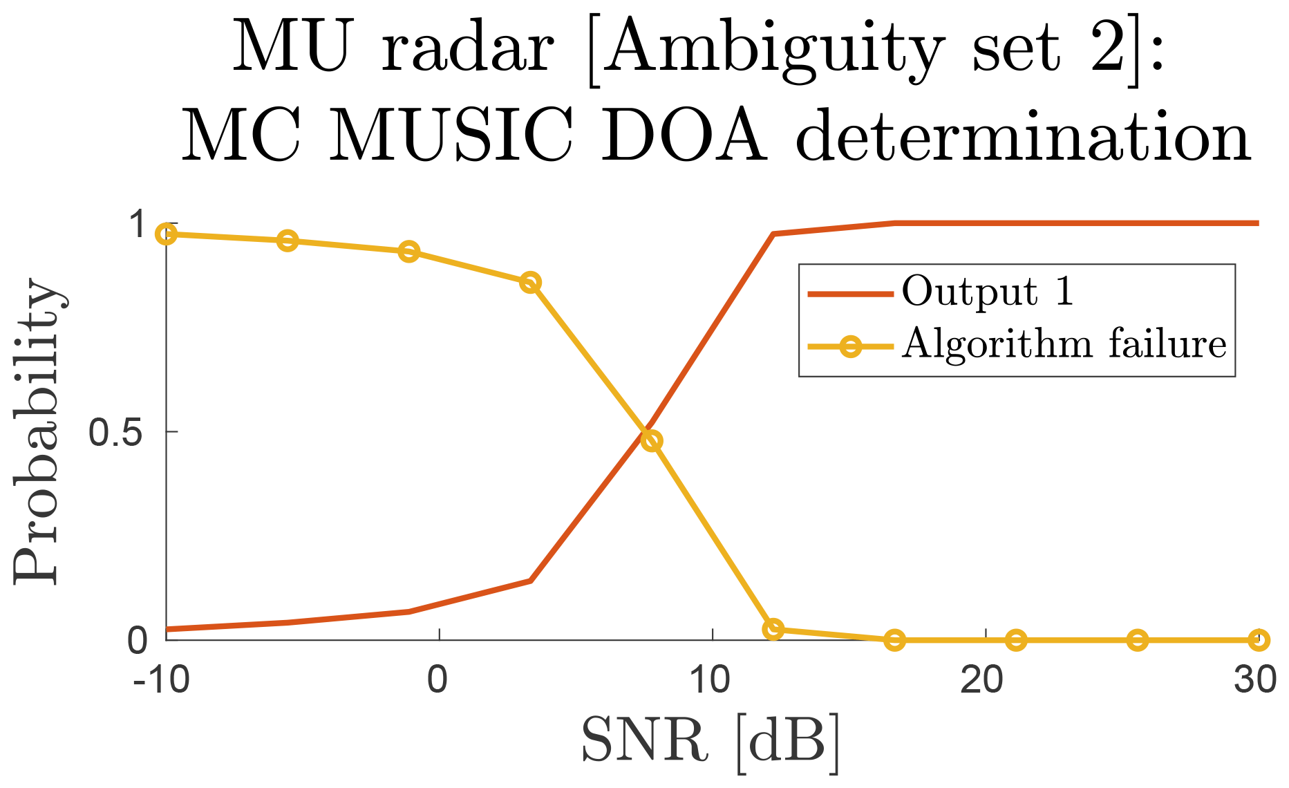
Figure 11The discretised output DOA distribution as a function of SNR and input DOA for the MU radar, using the subgroup model where input 1 is kII (ΩX) and output 1 is also kII (ΩY).
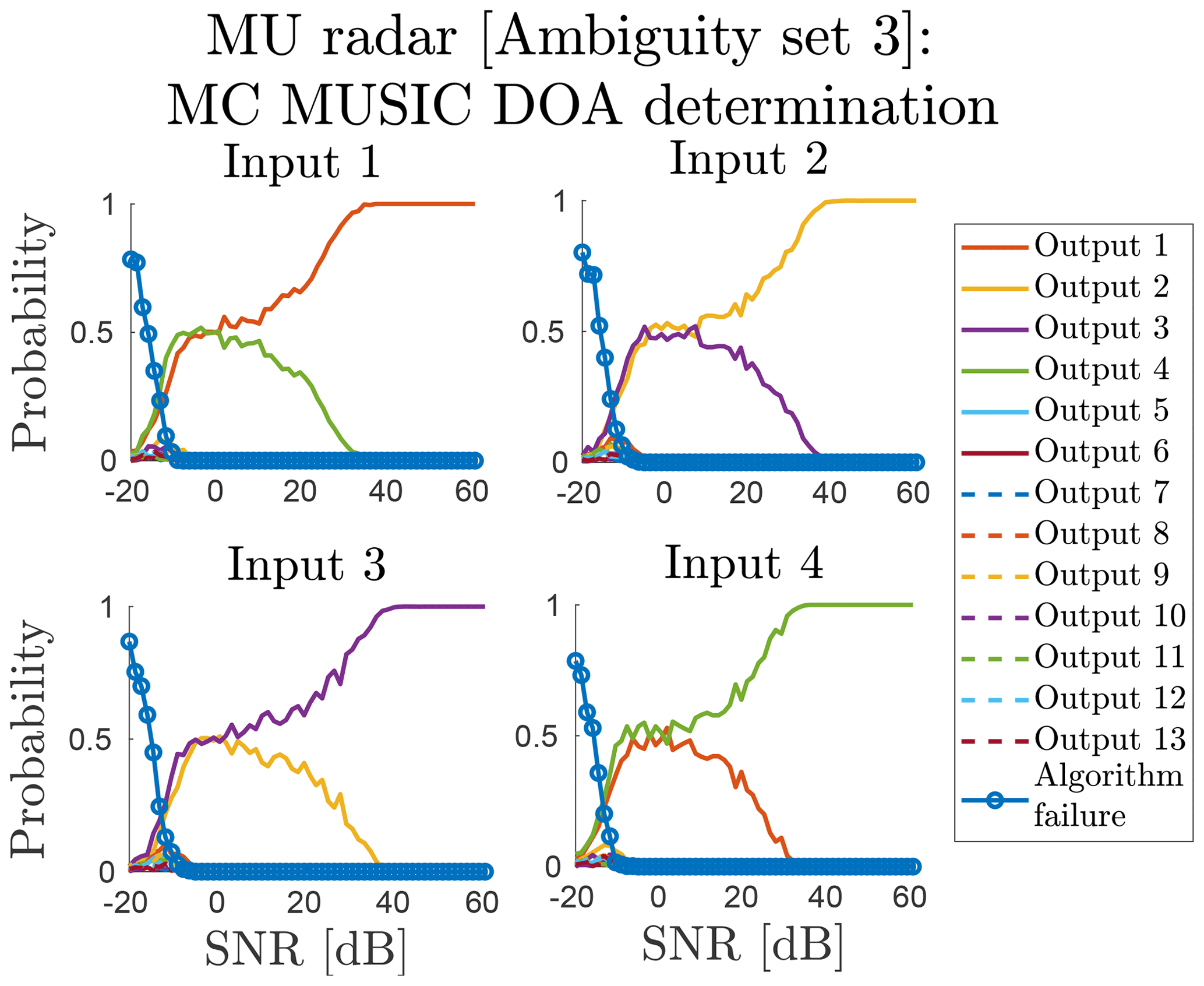
Figure 12The discretised output DOA distribution as a function of SNR and input DOA for the MU radar, using the subgroup model and kIII to generate ΩX and ΩY. The numerical values of inputs 1–4 (ΩX and corresponding to outputs 1–4) are given in Table 1; MU; III. 1–4.
As the phase centre model and subgroup model converge towards the zenith, we only present MC results from the subgroup model. The summary of the MC MUSIC DOA determinations for that model is illustrated for kI, kII and kIII in Figs. 10, 11 and 12, respectively.
From Fig. 10 we see trouble with determining directions uniquely if they are in the dark zone indicated by the MU panel in Fig. 6. The input and output locations are given by Fig. 8. Here, the MUSIC DOA determination is unable to select the correct output for input 5 and 6, even though there is a small difference between the signals (d=0.999988, as mentioned previously). As these simulations were using a single starting point for the MUSIC gradient ascent, the behaviour could be caused by a narrow peak problem. When using a fixed grid to select the starting point for the MUSIC gradient ascent, it may miss a narrow peak.
To test if a narrow peak was causing problems, we applied the parallel gradient ascent technique described in Sect. 3 when performing MC simulations for kIII. We chose the N=20 largest grid points with a minimum separation of δX=0.1 as initial conditions for the gradient ascents. We also increased the examined SNR range to find the region in which a d=0.999988 ambiguity could be correctly determined. The resulting MC statistics are illustrated in Fig. 12. For targets with SNR higher than 40 dB, an unambiguous DOA determination in this region is possible. Candidates for producing such strong echoes include bolides with large radar cross sections and active satellites.
As in Fig. 6a, all directions located close to the zenith are very robustly determinable. Therefore, no extensive MC simulations are needed for kII. Instead, we ran a set of sparse simulations in the SNR space to examine the onset of algorithm failure, illustrated in Fig. 11. In this case, the onset occurs below around 12 dB SNR.
The different input locations differ significantly in the SNR needed for stable DOA determination. This SNR limit also differs with respect to the used sensor response model. As such, the MUSIC peak value is a more stable quality indicator than SNR for DOA determination. The MUSIC peak value directly describes how well the used sensor response model matches the measured signal. The MUSIC peak distribution for the MU sub-array model simulations is given in Fig. 13. The simulations are the same as those illustrated in Fig. 11. In the SNR range (SNR ≲10 dB) where the MUSIC peak value appears to be independent of SNR, the algorithm cannot find any significant matches. The SNR region just above the flat section of the distribution is where ambiguities can occur. Measured echoes deviating from this relation between SNR and MUSIC peak value indicate an erroneous sensor response model.
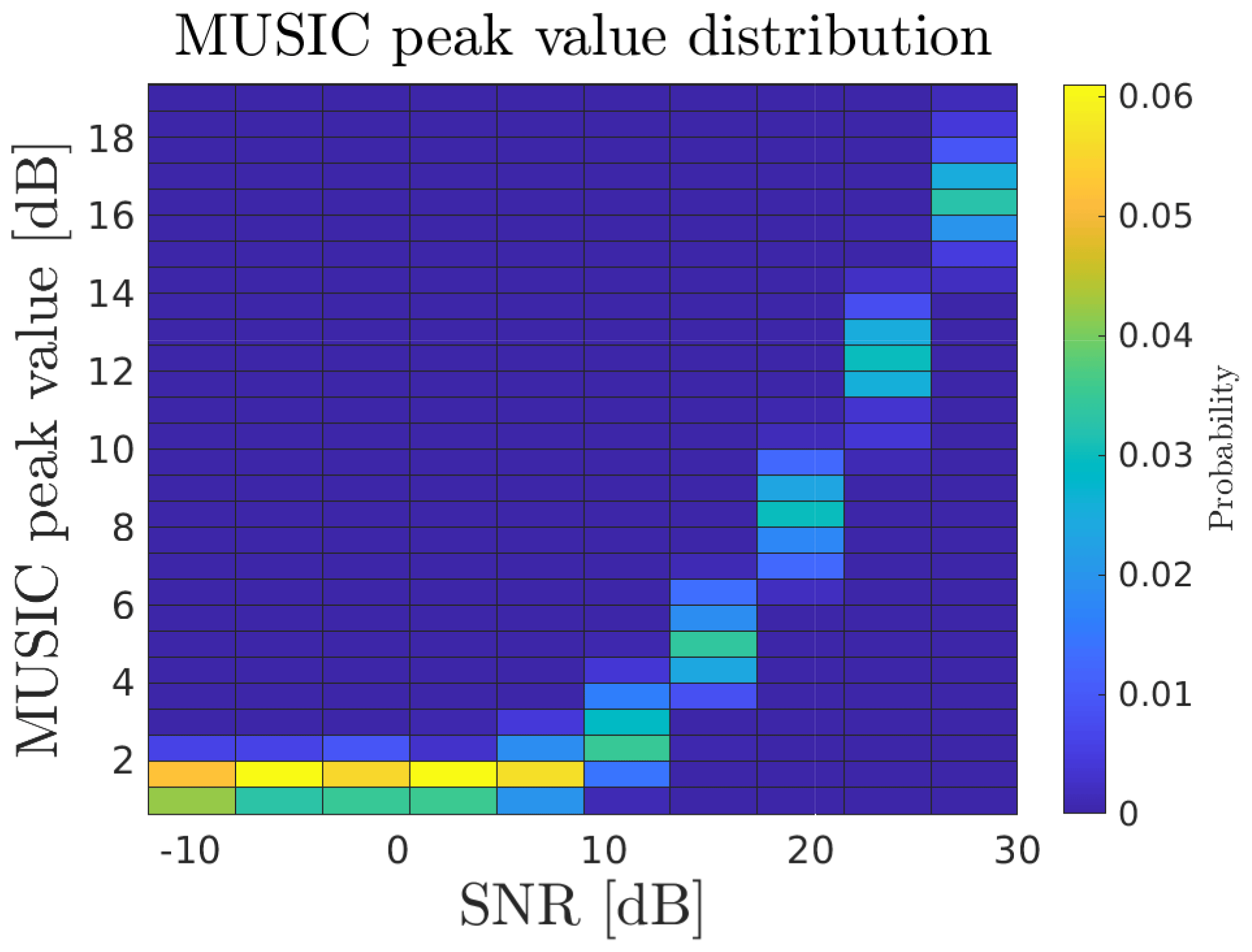
Figure 13Distribution of MUSIC peak values as a function of SNR compiled from all MU subgroup model MC simulations, with the zenith as the input DOA (see Fig. 11).
As the MU radar is a more complex system than the Jones 2.5λ radar, it might be misleading to simulate Bayesian inference, and we have therefore not done so. Also, the results indicate that for many directions ambiguities are not relevant.
5.3 MAARSY radar
The MAARSY radar system is limited to 16 output channels but with a flexible subgroup configuration. Studies looking at the interferometry of meteor echoes with MAARSY have predominantly used two different configurations. These configurations are illustrated in Figs. 4 and 5, and we hereafter refer to the them as MAARSY eight channel (Schult et al., 2013) and MAARSY 15 channel (Schult et al., 2017).
The phase centre model of the MAARSY eight channel configuration contains many perfect ambiguities. In this antenna configuration, all subgroups contain reflection symmetry lines, which means that their individual subgroup gains do not resolve ambiguities. However, the MAARSY eight channel configuration also contains the entire array as one of the channels. This channel has a significantly different gain pattern compared to the other channels. This creates a small shift in the sensor response between different directions. We have neither included an illustration of the ambiguity analysis of the phase centre model nor the subgroup model for the MAARSY eight channel configuration as they are trivial and ambiguous.
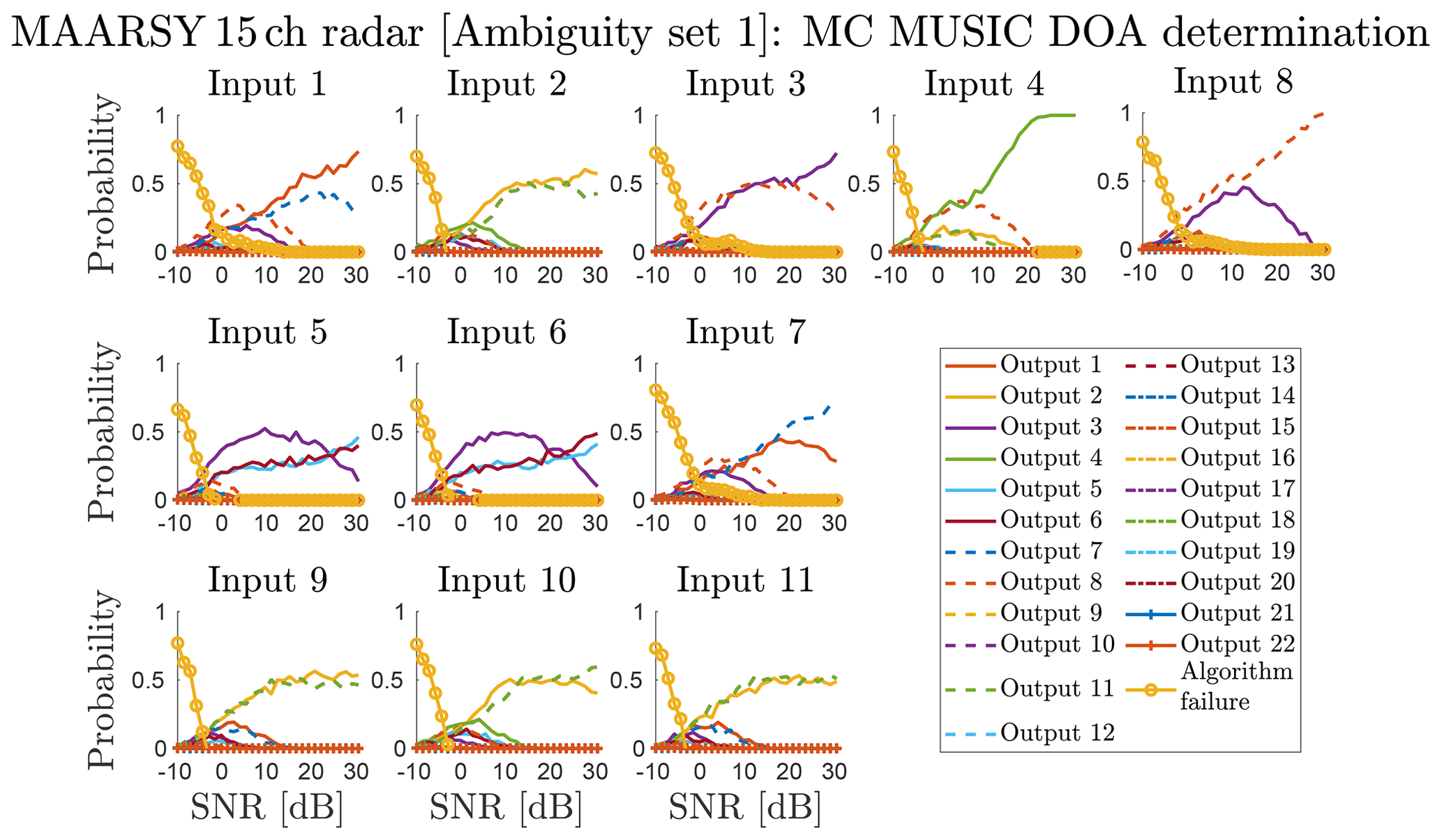
Figure 14The discretised output DOA distribution as a function of SNR and input DOA for the MAARSY 15 channel radar, using the subgroup model and kI to generate ΩX and ΩY. The numerical values of inputs 1–11 (ΩX and corresponding to outputs 1–11) are given in Table 1; MAARSY 15 channel; I.1–11.
For the phase centre model of the MAARSY 15 channel configuration, there are many close-to-perfect ambiguities and a few perfect ones. The distribution of ambiguities is close to identical to the MAARSY eight channel one. The addition of the smaller hexagonal subgroups, illustrated in Fig. 5, creates a decent basis for being able to determine a trajectory uniquely. But, in practice, if no assumptions are applied to restrict the DOA, our results such as, for example, Fig 14 indicate that it works reliably only for high-SNR targets.
In the MAARSY 15 channel configuration, half of the channels have vastly different antenna gain patterns. This fact makes the configuration better when the subgroup model is applied. We do not present any MC simulations for the phase centre model of the MAARSY 15 channel configuration but focus on the subgroup model.
In Fig. 6c, the sweep of worst ambiguity as a function of input DOA is illustrated. There are still a significant number of input DOAs that produce large inner-product ambiguities using this configuration. Considering the stability inside the main lobe, as indicated by the inner circle, and the distribution and severity at lower elevations, one can expect interferometric capabilities for a large portion of all meteor head echo events.
A significant complication was discovered regarding the application of the MUSIC algorithm on the MAARSY 15 channel subgroup model in that the vast differences in gain between channels narrow down the peaks in the MUSIC spectrum significantly. This is usually a desirable property as it allows more precise DOA determination. However, if the narrowing is extreme, a simple grid search for a peak will become unreasonably costly in terms of computations. As the difference in gain between the channels increases with zenith angle, the narrowing is a function of elevation, thus making low-elevation sources harder to determine with grid methods.
A peak at 45∘ elevation from a 10 dB SNR echo would have a peak width that requires a 3×105 by 3×105 point grid (i.e. 9×10¹⁰ points) to be robustly discovered, as opposed to the 200×200 point grid we have used for the MU radar.
As such, we applied the multiple gradient ascent method described in Sect. 3. This proved to be successful for solving the narrow peak problem of MAARSY with a N=50 and δX=0.1 for all tested cases.
The most prominent problem for DOA determination of echoes in the zenith with the MAARSY 15 channel configuration is that they are ambiguous with many DOAs below 57∘ elevation. If one can restrict the DOA to high elevations, a DOA determination algorithm should be fairly robust with respect to correctly identifying the correct direction. This is also supported by the MC simulations of this configuration. As the results are very similar for kI, kII and kIII, only the summary results for the kI simulations, without any elevation restriction, are illustrated in Fig. 14.
We also simulated a case in which an elevation restriction was added to the DOA determination algorithm. It was found that if the algorithm could be restricted to only accept matches above 70∘ elevation by some reasonable arguments or using a priori data, DOA determination for kI would be stable above 15 dB SNR.
For kIII, as illustrated in Fig. 6, the DOA determination suffers the same problem as the MU radar using the subgroup model because there are perfect ambiguities at low elevations. The general DOA determination performance is worse for the MAARSY 15 channel configuration than the MU radar, but they still display very similar behaviour for kIII. The actual value for the ambiguity is d=0.9999994, i.e 20 times closer to one than for the MU radar. It is unrealistic to expect this ambiguity to be resolved within any reasonable SNR for low-elevation DOAs.
5.4 PANSY radar
The PANSY radar is a special and interesting case when it comes to DOA determination. Firstly, all antennas are distributed vertically, ranging between −2 and +8 m. The distribution is asymmetric also within the subgroups themselves. Secondly, as is illustrated in Fig. 4, the radar is split into five larger collections of subgroups. These disjointed collections are of different sizes and shapes and located relatively far apart. This radar configuration would not be analysable with conventional ambiguity analysis methods due to its complexity. These reasons also make the subgroup gain patterns even more important, and a phase centre approximation would be outright unphysical to consider. Thus, we do not present any results for the phase centre model. Examining the ambiguity results for the subgroup model show very promising DOA determination capabilities. However, we can also see a potential problem with DOA determination algorithms due to the bumpiness of the surface. Therefore, we have applied the scattered gradient ascent method with the same configuration as for MAARSY.
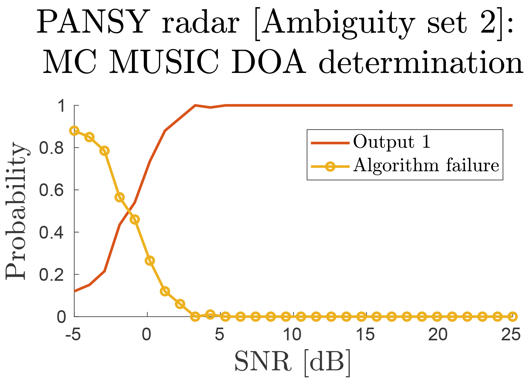
Figure 15The discretised output DOA distribution as a function of SNR and input DOA for the PANSY radar, using the subgroup model where input 1 is kII (ΩX) and output 1 is also kII (ΩY).
The MC DOA determination simulation summary for kII is illustrated in Fig. 15. The results for kI and kIII are practically identical to the results for kII but have shifted in SNR space. Examining these summary results shows that there is no need to perform the Bayesian analysis. Ambiguities are not prevalent enough, and usually only one clustering forms in low-SNR conditions. Instead of ambiguities affecting the quality of DOA determinations, sensor response model errors should to be most problematic for PANSY meteor head echo observations as the system setup varies over time due to Antarctic conditions.
5.5 PANSY meteor radar
We only present summary results for the PANSY 2.5λ meteor receiver system as the very similar standard Jones 2.5λ system results have been covered in Sect. 5.1. Since the antennas are placed at the appropriate distances for a Jones 2.5λ radar in the x–y plane but displaced in the z direction, the actual distances between the antennas are slightly larger than a standard Jones 2.5λ system. Also, as it is not a planar array, the ambiguity situation is dependant on input DOA, as shown in Appendix B. As such it was also included in the ambiguity sweeps in Fig. 6.
To summarise the comparison between the standard Jones 2.5λ and the PANSY 2.5λ receiver, the system performs better then the standard system for DOAs originating from south–east but performs worse for the opposite direction. The MC simulations for this system is basically equivalent to the standard system but slightly shifted in SNR space. The magnitudes of these shifts are equal to the differences of the SNR limits given in Table 1.
The main purpose of the ambiguity analysis and the MC DOA determination simulations was to provide improved understanding of DOA determination dynamics. These results and methods provide simulated theoretical references that are useful when analysing real measurement data.
We compared the phase centre models and subgroup models for the MU, PANSY and MAARSY radars. For the MU radar, even though the subgroup model has ambiguities at low elevations, this is the expected behaviour in real data as well. Its performance in terms of limiting SNR is also better than the phase centre model. As such, the subgroup model is overall the better choice. For the PANSY radar the situation is similar as the phase centre model is outright nonphysical and should not be used. In the case of MAARSY, if the DOA search is restricted to high elevations, either model is sufficient.
The simulations also provided insight into the construction of DOA determination algorithms. It was shown for the MAARSY, MU and PANSY systems that an additional step of a scattered gradient ascent had to be implemented due to the topology of the MUSIC function. The success of this method suggests that there may be other optimisation algorithms that could further improve performance, such as the bird swarm algorithm (Meng et al., 2016).
The comparison between a standard Jones 2.5λ system and the PANSY meteor radar showed slight performance differences, especially in the limiting SNR as a function of input DOA. This knowledge can help calibrate thresholds for future data analysis pipelines. The comparison showed the advantage of doing ambiguity analysis and MC simulation prior to the construction of such pipelines as it reveals the expected DOA determination performance of a system.
Considering the application of these methods and results on measurement data, they provide a reference, not only for SNR limits but also for model validation. If measurements do not follow the dynamics simulated by these methods, assuming the pipeline itself is validated and stable, it points towards the models not representing reality. This makes such simulations a good validation tool for analysis pipelines. For example, it has been frequently shown that multiple-receiver radar systems are in need of phase calibrations (e.g. Chau et al., 2014). In the case of the results presented here, the dynamics would all be modified to some degree if one would add constant phase offsets to each receiver in our models (see Appendix A). The framework of DOA determination simulation provides a possibility to test these matters.
We have explored a Bayesian approach to determine the most probable DOA of a target given several measurements distributed among noise-induced ambiguities. Such an approach can be applied if it is not possible to increase the SNR using coherent integration. The results indicate that this is a suitable method for providing a quantitative probability for which DOA is correct. Using the Bayesian method, it appears possible to analyse echoes down to 4 dB SNR for both the standard Jones 2.5λ radar and the PANSY meteor radar, given enough independent data points from the same target.
Lastly, the MC simulations in this paper demonstrated quantitatively that ambiguities are more or less relevant, depending on radar system configurations. In systems where ambiguities are not prevalent, the DOA determination failure onset is the important variable to determine. In systems where noise-induced ambiguities are relevant, it is important to determine the SNR range in which they emerge. Our results show that the PANSY system is not affected by noise-induced ambiguities, while the MU radar has a small region of SNRs where they could be relevant. The Jones-type systems and MAARSY all have relevant noise-induced ambiguities.
Table 1 contains all the MC simulations performed in our study, collected in terms of limiting SNR and input DOA. Any DOA determination on data with SNR above the limiting value will provide the correct output DOA with >99% confidence.
Using interferometric radar systems to perform meteor head echo measurements, the trajectory can be directly determined (e.g. Kero et al., 2012b). Techniques like the ones presented here can be employed to avoid misclassifying the DOA and, thereby, avoiding nonphysical results. For example, the existence of high-altitude radar meteors is still an open question (Gao and Mathews, 2015; Kero et al., 2019). Some previous studies have been centred on the low probability of side lobe detections as the explanation (e.g Vierinen et al., 2014). With interferometric systems, this question could be further addressed using these methods.
Adding a phase offset to each element in the subgroups defined in Eq. (32) gives the following:
Inserting the phase offset subgroup model from Eq. (A1) into Eq. (31), the explicit form of the inner product calculation in Eq. (6) becomes the following:
Here, ∗ denotes complex conjugation. This form is valid for all possible phase offsets, including radars with and without subgroups. Using matrix algebra, Eq. (A2) can be rewritten as follows:
where
If Nj=1, i.e. single-antenna channels, then the vectors in Eq. (A3) become scalars and the phase offsets wj are commutative. Thus, and wj cancel to 1. As they cancel, the phase offsets do not impact d(k). Therefore, phase offsets do not impact the ambiguity dynamics.
Additionally, if ϕjl=ϕj, i.e. phase offsets are independent of antenna in a subgroup, then . The is a scalar and is commutative. Thus, can be moved to cancel , and phase offsets do not impact d(k). In all other cases, the phase offsets will affect d(k) and change the ambiguity dynamics of a system.
The results are the same if the ambiguity indicator d is defined without the absolute value or if the distance is used.
What follows is a derivation of the fact that planar arrays with single-antenna channels are uniquely identified by a single translated ambiguity map.
Inserting Eq. (30) into the inner product calculation in Eq. (6) gives the following:
Equation (B1) shows, that for the phase centre model, a singular function will define the morphology of the ambiguity map which is only translated in k space. The k vectors only move on the surface of a sphere in 3D. When the set of rj vectors are planar, the translations become linear in 2D. However, if the set of rj are not planar, the projection down to 2D becomes non-linear, and the ambiguity maps are no longer simple translations of the base function.
The results are the same if the ambiguity indicator d is defined without the absolute value or if the distance is used.
All the data used in this manuscript were generated by the authors and are available from the Swedish National Data (SND) service findable, accessible, interoperable and reusable (FAIR) repository at https://doi.org/10.5878/hcdz-2j74 (Kastinen and Kero, 2020).
An animation of the simulated MC DOA determination at different SNRs for the MU radar subgroup model (with array SNR in the range from −30 to 10 dB) is available at the SND repository (https://doi.org/10.5878/hcdz-2j74, Kastinen and Kero, 2020).
DK developed the model code and performed the simulations. DK prepared the paper with contributions from JK.
The authors declare that they have no conflict of interest.
We thank Koji Nishimura for providing the PANSY radar antenna configuration data, Taishi Hashimoto for providing the PANSY meteor radar antenna configuration data and Carsten Schult for providing the MAARSY radar antenna configuration data.
This paper was edited by Jorge Luis Chau and reviewed by two anonymous referees.
Bianchi, C. and Meloni, A.: Natural and man-made terrestrial electromagnetic noise: an outlook, Ann. Geophys.-Italy, 50, 435–445, 2007. a
Campbell-Brown, M. D.: Solar cycle variation in radar meteor rates, MNRAS, 485, 4446–4453, https://doi.org/10.1093/mnras/stz697, 2019. a
Ceplecha, Z., Borovička, J., Elford, W. G., Revelle, D. O., Hawkes, R. L., Porubčan, V., and Šimek, M.: Meteor Phenomena and Bodies, Space Sci. Rev., 84, 327–471, https://doi.org/10.1023/A:1005069928850, 1998. a
Chau, J. L. and Clahsen, M.: Empirical Phase Calibration for Multistatic Specular Meteor Radars Using a Beamforming Approach, Radio Sci., 54, 60–71, https://doi.org/10.1029/2018RS006741, 2019. a, b, c, d, e
Chau, J. L. and Woodman, R. F.: Observations of meteor-head echoes using the Jicamarca 50MHz radar in interferometer mode, Atmos. Chem. Phys., 4, 511–521, https://doi.org/10.5194/acp-4-511-2004, 2004. a
Chau, J. L., Renkwitz, T., Stober, G., and Latteck, R.: MAARSY multiple receiver phase calibration using radio sources, J. Atmos. Sol.-Terr. Phy., 118, 55–63, 2014. a, b, c, d
Close, S., Hunt, S. M., Minardi, M. J., and McKeen, F. M.: Analysis of Perseid meteor head echo data collected using the Advanced Research Projects Agency Long-Range Tracking and Instrumentation Radar (ALTAIR), Radio Sci., 35, 1233–1240, https://doi.org/10.1029/1999RS002277, 2000. a
Ferreol, A., Larzabal, P., and Viberg, M.: On the asymptotic performance analysis of subspace DOA estimation in the presence of modeling errors: case of MUSIC, IEEE T. Signal Proces., 54, 907–920, 2006. a
Fujiwara, Y., Kero, J., Abo, M., Szasz, C., and Nakamura, T.: MU radar head echo observations of the 2012 October Draconid outburst, Mon. Not. R. Astron. Soc., 455, 3273–3280, 2016. a
Fukao, S., Sato, T., Tsuda, T., Kato, S., Wakasugi, K., and Makihira, T.: The MU radar with active phased array system. I - Antenna and power amplifiers. II - In-house equipment, Radio Sci., 20, 1155–1176, https://doi.org/10.1029/RS020i006p01155, 1985. a
Gao, B. and Mathews, J. D.: High-altitude radar meteors observed at Jicamarca Radio Observatory using a multibaseline interferometric technique, MNRAS, 452, 4252–4262, https://doi.org/10.1093/mnras/stv1548, 2015. a
Hashimoto, T., Saito, A., Nishimura, K., Tsutsumi, M., Sato, K., and Sato, T.: First Incoherent Scatter Measurements and Adaptive Suppression of Field-Aligned Irregularities by the PANSY Radar at Syowa Station, Antarctic, J.Atmos. Ocean. Tech., 36, 1881–1888, https://doi.org/10.1175/JTECH-D-18-0175.1, 2019. a
Hassenpflug, G., Yamamoto, M., Luce, H., and Fukao, S.: Description and demonstration of the new Middle and Upper atmosphere Radar imaging system: 1-D, 2-D, and 3-D imaging of troposphere and stratosphere, Radio Sci., 43, RS2013, https://doi.org/10.1029/2006RS003603, 2008. a
Hocking, W. K.: A new approach to momentum flux determinations using SKiYMET meteor radars, Ann. Geophys., 23, 2433–2439, https://doi.org/10.5194/angeo-23-2433-2005, 2005. a
Hocking, W. K., Fuller, B., and Vandepeer, B.: Real-time determination of meteor-related parameters utilizing modern digital technology, J. Atmos. Sol.-Terr. Phy., 63, 155–169, https://doi.org/10.1016/S1364-6826(00)00138-3, 2001. a, b, c
Holdsworth, D. A.: Angle of arrival estimation for all-sky interferometric meteor radar systems, Radio Sci., 40, RS6010, https://doi.org/10.1029/2005RS003245, 2005. a
Jones, J., Webster, A. R., and Hocking, W. K.: An improved interferometer design for use with meteor radars, Radio Sci., 33, 55–65, https://doi.org/10.1029/97RS03050, 1998. a, b, c, d, e, f, g, h, i, j, k, l
Jones, J., Brown, P., Ellis, K. J., Webster, A. R., Campbell-Brown, M., Krzemenski, Z., and Weryk, R. J.: The Canadian Meteor Orbit Radar: system overview and preliminary results, Planet. Space Sci., 53, 413–421, https://doi.org/10.1016/j.pss.2004.11.002, 2005. a
Kangas, A., Stoica, P., and Soderstrom, T.: Finite sample and modelling error effects on ESPRIT and MUSIC direction estimators, IEE P.-Radar Son. Nav., 141, 249–255, 1994. a
Kangas, A., Stoica, P., and Söderström, T.: Large-sample analysis of MUSIC and Min-Norm direction estimators in the presence of model errors, Circ. Syst. Signal Pr., 15, 377–393, 1996. a
Kastinen, D.: Determining all ambiguities in direction of arrival measured by radar systems, Radio Sci. Bull., 333, 3–33, 2018. a, b, c, d
Kastinen, D. and Kero J.: Probabilistic analysis of ambiguities in radar echo direction of arrival from meteors, Version 1, Swedish Institute of Space Physics, Solar terrestrial and atmospheric research programme, Swedish National Data Service, https://doi.org/10.5878/hcdz-2j74, 2020. a, b
Kastinen, D. and Kero, J.: A Monte Carlo-type simulation toolbox for Solar System small body dynamics: Application to the October Draconids, Planet. Space Sci., 143, 53–66, https://doi.org/10.1016/j.pss.2017.03.007, 2017. a, b
Kero, J., Szasz, C., Nakamura, T., Terasawa, T., Miyamoto, H., and Nishimura, K.: First results from the 2009–2010 MU radar head echo observation programme for sporadic and shower meteors: the Orionids 2009, Mon. Not. R. Astron. Soc., 416, 2550–2559, https://doi.org/10.1111/j.1365-2966.2011.19146.x, 2011. a
Kero, J., Szasz, C., Nakamura, T., Meisel, D. D., Ueda, M., Fujiwara, Y., Terasawa, T., Miyamoto, H., and Nishimura, K.: The 2009–2010 MU radar head echo observation programme for sporadic and shower meteors: radiant densities and diurnal rates., Mon. Not. R. Astron. Soc., 425, 135–146, https://doi.org/10.1111/j.1365-2966.2012.21407.x, 2012a. a
Kero, J., Szasz, C., Nakamura, T., Terasawa, T., Miyamoto, H., and Nishimura, K.: A meteor head echo analysis algorithm for the lower VHF band, Ann. Geophys., 30, 639–659, https://doi.org/10.5194/angeo-30-639-2012, 2012b. a, b, c, d, e, f
Kero, J., Szasz, C., and Nakamura, T.: MU head echo observations of the 2010 Geminids: radiant, orbit, and meteor flux observing biases, Ann. Geophys., 31, 439–449, https://doi.org/10.5194/angeo-31-439-2013, 2013. a
Kero, J., Campbell-Brown, M. D., Stober, G., Chau, J. L., Mathews, J. D., and Pellinen-Wannberg, A.: Radar Observations of Meteors, in: Meteoroids: Sources of Meteors on Earth and Beyond, edited by: Ryabova, G. O., Asher, D. J., and Campbell-Brown, M. J., Cambridge University Press, UK, 65–89, 2019. a, b
Kildal, P.-S.: Foundations of antenna engineering: a unified approach for line-of-sight and multipath, chap. Terminology, quantities, units and symbols, Kildal Antenn AB, Gothenburg, Sweden, 7–11, 2015. a
Latteck, R., Singer, W., Rapp, M., and Renkwitz, T.: MAARSY – the new MST radar on Andøya/Norway, Adv. Radio Sci., 8, 219–224, https://doi.org/10.5194/ars-8-219-2010, 2010. a
McCrea, I., Aikio, A., Alfonsi, L., Belova, E., Buchert, S., Clilverd, M., Engler, N., Gustavsson, B., Heinselman, C., Kero, J., Kosch, M., Lamy, H., Leyser, T., Ogawa, Y., Oksavik, K., Pellinen-Wannberg, A., Pitout, F., Rapp, M., Stanislawska, I., and Vierinen, J.: The science case for the EISCAT_3D radar, Progress in Earth and Planetary Science, 2, 21, https://doi.org/10.1186/s40645-015-0051-8, 2015. a
Meng, X.-B., Gao, X. Z., Lu, L., Liu, Y., and Zhang, H.: A new bio-inspired optimisation algorithm: Bird Swarm Algorithm, J. Exp. Theor. Artif. In., 28, 673–687, 2016. a
Nishimura, K., Sato, T., Nakamura, T., and Ueda, M.: High sensitivity radar-optical observations of faint meteors, IEICE Trans. Comm., E84-C, 1877–1884, 2001. a
Polisensky, E.: LFmap: A low frequency sky map generating program, Long Wavelength Array Memo 111, available at: https://www.faculty.ece.vt.edu/swe/lwa/ (last access: March 2019), 2007. a
Renkwitz, T., Singer, W., Latteck, R., Stober, G., and Rapp, M.: Validation of the radiation pattern of the Middle Atmosphere Alomar Radar System (MAARSY), Adv. Radio Sci., 10, 245–253, https://doi.org/10.5194/ars-10-245-2012, 2012. a
Renkwitz, T., Stober, G., Latteck, R., Singer, W., and Rapp, M.: New experiments to validate the radiation pattern of the Middle Atmosphere Alomar Radar System (MAARSY), Adv. Radio Sci., 11, 283–289, https://doi.org/10.5194/ars-11-283-2013, 2013. a
Renkwitz, T., Schult, C., Latteck, R., and Stober, G.: Validation of the radiation pattern of the VHF MST radar MAARSY by scattering off a sounding rocket's payload, Adv. Radio Sci., 13, 41–48, https://doi.org/10.5194/ars-13-41-2015, 2015. a
Renkwitz, T., Schult, C., and Latteck, R.: VHF antenna pattern characterization by the observation of meteor head echoes, Atmos. Meas. Tech., 10, 527–535, https://doi.org/10.5194/amt-10-527-2017, 2017. a
Sato, K., Tsutsumi, M., Sato, T., Nakamura, T., Saito, A., Tomikawa, Y., Nishimura, K., Kohma, M., Yamagishi, H., and Yamanouchi, T.: Program of the Antarctic Syowa MST/IS radar (PANSY), J. Atmos. Sol.-Terr. Phys., 118, 2–15, https://doi.org/10.1016/j.jastp.2013.08.022, 2014. a, b
Schmidt, R. O.: Multiple emitter location and signal parameter estimation, IEEE T. Antenn. Propag., 34, 276–280, https://doi.org/10.1109/TAP.1986.1143830, 1986. a, b, c, d
Schult, C., Stober, G., Chau, J. L., and Latteck, R.: Determination of meteor-head echo trajectories using the interferometric capabilities of MAARSY, Ann. Geophys., 31, 1843–1851, https://doi.org/10.5194/angeo-31-1843-2013, 2013. a, b, c
Schult, C., Stober, G., Janches, D., and Chau, J. L.: Results of the first continuous meteor head echo survey at polar latitudes, Icarus, 297, 1–13, https://doi.org/10.1016/j.icarus.2017.06.019, 2017. a, b, c
Szasz, C., Kero, J., Meisel, D. D., Pellinen-Wannberg, A., Wannberg, G., and Westman, A.: Orbit characteristics of the tristatic EISCAT UHF meteors, Mon. Not. R. Astron. Soc., 388, 15–25, https://doi.org/10.1111/j.1365-2966.2008.13374.x, 2008. a
Vaubaillon, J., Colas, F., and Jorda, L.: A new method to predict meteor showers. I. Description of the model, Astron. Astrophys., 439, 751–760, https://doi.org/10.1051/0004-6361:20041544, 2005a. a
Vaubaillon, J., Colas, F., and Jorda, L.: A new method to predict meteor showers. II. Application to the Leonids, Astron. Astrophys., 439, 761–770, https://doi.org/10.1051/0004-6361:20042626, 2005b. a
Vierinen, J., Fentzke, J., and Miller, E.: An explanation for observations of apparently high-altitude meteors, MNRAS, 438, 2406–2412, https://doi.org/10.1093/mnras/stt2358, 2014. a
Whipple, F. L.: A Comet Model. II. Physical Relations for Comets and Meteors., Astrophys. J., 113, 464, https://doi.org/10.1086/145416, 1951. a
Younger, J. P. and Reid, I. M.: Interferometer angle-of-arrival determination using precalculated phases, Radio Sci., 52, 1058–1066, https://doi.org/10.1002/2017RS006284, 2017. a, b
- Abstract
- Introduction
- Method
- DOA determination
- Radar systems
- Results
- Conclusions
- Appendix A: Impact of known phase offsets on ambiguities
- Appendix B: Ambiguities of planar arrays with single-antenna channels
- Data availability
- Video supplement
- Author contributions
- Competing interests
- Acknowledgements
- Review statement
- References