the Creative Commons Attribution 4.0 License.
the Creative Commons Attribution 4.0 License.
 | 16 Dec 2020
Absolute calibration method for frequency-modulated continuous wave (FMCW) cloud radars based on corner reflectors
Felipe Toledo
Julien Delanoë
Martial Haeffelin
Jean-Charles Dupont
Susana Jorquera
Christophe Le Gac
This article presents a new cloud radar calibration methodology using solid reference reflectors mounted on masts, developed during two field experiments held in 2018 and 2019 at the Site Instrumental de Recherche par Télédétection Atmosphérique (SIRTA) atmospheric observatory, located in Palaiseau, France, in the framework of the Aerosol Clouds Trace gases Research InfraStructure version 2 (ACTRIS-2) research and innovation program.
The experimental setup includes 10 and 20 cm triangular trihedral targets installed at the top of 10 and 20 m masts, respectively. The 10 cm target is mounted on a pan-tilt motor at the top of the 10 m mast to precisely align its boresight with the radar beam. Sources of calibration bias and uncertainty are identified and quantified. Specifically, this work assesses the impact of receiver compression, temperature variations inside the radar, frequency-dependent losses in the receiver's intermediate frequency (IF), clutter and experimental setup misalignment. Setup misalignment is a source of bias, previously undocumented in the literature, that can have an impact of the order of tenths of a decibel in calibration retrievals of W-band radars.
A detailed analysis enabled the quantification of the importance of each uncertainty source to the final cloud radar calibration uncertainty. The dominant uncertainty source comes from the uncharacterized reference target which reached 2 dB. Additionally, the analysis revealed that our 20 m mast setup with an approximate alignment approach is preferred to the 10 m mast setup with the motor-driven alignment system. The calibration uncertainty associated with signal-to-clutter ratio of the former is 10 times smaller than for the latter.
Following the proposed methodology, it is possible to reduce the added contribution from all uncertainty terms, excluding the target characterization, down to 0.4 dB. Therefore, this procedure should enable the achievement of calibration uncertainties under 1 dB when characterized reflectors are available.
Cloud radar calibration results are found to be repeatable when comparing results from a total of 18 independent tests. Once calibrated, the cloud radar provides valid reflectivity values when sampling midtropospheric clouds. Thus, we conclude that the method is repeatable and robust, and that the uncertainties are precisely characterized. The method can be implemented under different configurations as long as the proposed principles are respected. It could be extended to reference reflectors held by other lifting devices such as tethered balloons or unmanned aerial vehicles.
- Article
(6024 KB) - Full-text XML
-
Supplement
(1192 KB) - BibTeX
- EndNote


Clouds remain, to this day, one of the major sources of uncertainty in future climate predictions (Boucher et al., 2013; Myhre et al., 2013; Mülmenstädt and Feingold, 2018). This arises partly from the wide range of scales involved in cloud systems, where a knowledge of cloud microphysics, particularly cloud–aerosol interactions, is critical for predicting large-scale phenomena such as cloud radiative forcing or precipitation.
To address this and other related issues, the Aerosol Clouds Trace gases Research InfraStructure (ACTRIS) is establishing a state-of-the-art ground-based observation network (Pappalardo, 2018). Within this organization, the Centre for Cloud Remote Sensing (CCRES) is in charge of creating and defining calibration and quality assurance protocols for the observation of cloud properties across the complete network.
One of the key instruments for cloud remote sensing stations is cloud radar. Cloud radars enable retrievals of several relevant parameters for cloud research including, but not limited to, liquid water and ice content profiles, cloud boundaries, cloud fraction, precipitation rate and turbulence (Fox and Illingworth, 1997; Hogan et al., 2001; Wærsted et al., 2017; Dupont et al., 2018; Haynes et al., 2009). Additionally, recent studies revealed the potential of cloud radars to support a better understanding of fog processes (Dupont et al., 2012; Boers et al., 2013; Wærsted et al., 2019).
However, calibration remains a crucial factor in the reliability of radar-retrieved data (Ewald et al., 2019). Systematic differences of 2 dB have already been observed, for example, between the satellite-based radar CloudSat and the Lindenberg microwave radar (MIRA) (Protat et al., 2009). This is a very important issue since calibration errors as small as 1 dB would already introduce uncertainties in liquid water and ice content retrievals of the order of 15 %–20 % (Fox and Illingworth, 1997; Ewald et al., 2019).
Since the objective of the CCRES is to guarantee a network of high-quality observations, it is essential to develop standardized and repeatable calibration methods for its instrumental network.
This paper presents an absolute calibration method for W-band radars. It has been developed based on results from two experimental calibration campaigns performed at the Site Instrumental de Recherche par Télédétection Atmosphérique (SIRTA) atmospheric observatory located in Palaiseau, France (Haeffelin et al., 2005). The SIRTA observatory hosts part of the ACTRIS CCRES infrastructure. For the experiments, we used a BASTA mini W-band frequency-modulated continuous wave (FMCW) radar with scanning capabilities (Delanoë et al., 2016). Nevertheless, the principles, procedures and limitations presented here should be applicable for any radar with similar characteristics, even when operating in another frequency band.
The method consists of an end-to-end calibration approach, which consists of retrieving the radar calibration coefficient by sampling the power reflected from a reference reflector mounted on top of a mast (Chandrasekar et al., 2015). A detailed analysis of uncertainty and bias sources is performed, with the objective of determining how to improve the experiment to reach a calibration uncertainty lower than 1 dB. This low uncertainty in the calibration would not only be useful for high-quality retrievals but would also enable the use of the radar as a reliable reference for calibration transfer to other ground- or space-based cloud radars (Bergada et al., 2001; Protat et al., 2011; Ewald et al., 2019).
The article is structured as follows: Sect. 2 presents the equations and theoretical considerations involved in the calibration exercise. Section 3 shows the experimental setup, complemented by Sect. 4 in which the experimental procedure and data treatment are presented. Section 5 presents an analysis of the sources of uncertainty and bias involved in our calibration experiment. Section 6 presents the final calibration results, the uncertainty budget and an analysis of the variability in the calibration bias correction, followed by the conclusions.
The absolute calibration of a radar consists of determining the radar cross section (RCS) calibration term CΓ and the radar equivalent reflectivity calibration term CZ. They enable the calculation of radar cross section Γ(r) (RCS) or radar equivalent reflectivity Ze, respectively, from the power backscattered by a punctual or distributed target towards the radar (Bringi and Chandrasekar, 2001).
Equation (2a) presents an expression for the RCS calibration term CΓ(T,Fb) of a FMCW radar as a function of its internal parameters. The deduction of this expression is shown in the Supplement. Gt and Gr are the maximum gains of the transmitting and receiving antennas, respectively, and are unitless. λ is the wavelength of the carrier wave in meters, and pt is the power emitted by the radar in milliwatts.
The gain of solid-state components changes with variations in their temperature. Thus, we make this dependence explicit in the receiver loss budget Lr(T,Fb) and in the transmitter loss budget Lt(T). Loss budgets are the product of all losses divided by the gain terms at the end of the receiver or emitter chain and are unitless.
Additionally, a range dependence is included in Lr(T,Fb) to account for variations in the receiver's intermediate frequency (IF) loss for different beat frequency Fb values. The beat frequency in FMCW radars is proportional to the distance between the instrument and the backscattering element (Delanoë et al., 2016). Thus, changes in the IF loss for different beat frequencies introduce a range-dependent bias. For the 12.5 m resolution mode used in this calibration exercise, Fb ranges between 168 and 180 MHz and can be related to r (in meters) using Eq. (1).
In theory, CΓ(T,Fb) can be calculated by characterizing the gains and losses of every component inside the radar system and adding them. This can be very challenging, depending on the complexity of the radar hardware and the available radio frequency analysis equipment. In addition, with this procedure it is not possible to quantify losses due to interactions between different components, especially changes in antenna alignment or radome degradation (Anagnostou et al., 2001). This motivates the implementation of an end-to-end calibration, which consists of the characterization of the complete radar system at once by using a reference reflector and Eq. (2b).
Equation (2b) links the calibration term CΓ(T,Fb) to the RCS Γ(r) of a target at a distance r. Γ(r) is expressed in units of decibels per square meter (dBsm), Lat(r) is the atmospheric attenuation between the object and the radar in decibels (dB), which can be calculated using a millimeter-wave attenuation model (e.g., Liebe, 1989). Pr(r) is the power received from the target in decibel milliwatts (dBm), and CΓ(T,Fb) is the RCS calibration term in . The unit is the abbreviation of decibels referenced as 1 m−2 mW−1. The units in the RCS calibration term compensate the radar power units, guaranteeing the retrieval of physical RCS values. The explicit temperature and range dependency of the calibration term has the function of compensating gain changes in Pr(r) introduced by temperature effects and variations in the IF loss with distance.
This principle can be used in an end-to-end calibration by installing a target with a known RCS Γ0 at a known distance r0 and sampling the power Pr(r0) reflected back to calculate CΓ(T,Fb). However, some additional considerations must be made to perform this retrieval.
In Eq. (2a), we state that the calibration value has a temperature and a range dependency. Experimental results indicate that the temperature dependency of CΓ(T,Fb) can be approximated by a linear relationship, as shown in Eq. (3). Here n is the temperature dependency term in dB ∘C−1, T the internal radar temperature in ∘C and T0 is a reference temperature value in degrees Celsius. More details about the temperature correction can be found in Sect. 5.4.
The range dependence of CΓ(T,Fb) is treated independently by defining a IF loss-correction function, fIF(Fb), in decibels. This function is introduced to compensate for relative loss variations at different IF frequencies. The IF loss-correction function is studied in Sect. 5.5.
From the aforementioned observations, we divide CΓ(T,Fb) into three components, as shown in Eq. (3). This separation consists of a constant calibration coefficient , in dB(m−2 mW−1), and the two correction functions n(T−T0) and fIF(Fb).
As fIF(Fb) corrects for relative variations in receiver loss with distance, we define fIF(F0)=0 at the IF frequency value F0, which is associated to the reflector position r0 (linked by Eq. 1). Using this and Eqs. (2b) and (3), we obtain Eqs. (4a) and (4b).
Equation (4a) shows how the calibration term CΓ(T,F0) at position r0 is related to the calibration coefficient and the temperature correction n(T−T0). Meanwhile, Eq. (4b) indicates how experimental Pr(r0) measurements can be associated with a CΓ(T,F0) value, using in situ information to calculate 2Lat(r0). Then, using Eq. (4a), we can compute by subtracting the temperature correction function n(T−T0). This temperature correction is derived independently in Sect. 5.4. Knowing and the temperature correction, CΓ(T,Fb) is calculated by adding the IF correction function, which is independently retrieved in Sect. 5.5.
Once CΓ(T,Fb) is known, we can calculate the radar equivalent reflectivity calibration term CZ(T,Fb), in dB(mm6 m−5 mW−1), with Eq. (5a) (Yau and Rogers, 1996). This relationship assumes that the radar has two identical parallel antennas with a Gaussian-shaped main lobe. θ is the antenna beamwidth in radians, mδr is the radar distance resolution in meters, and is the dielectric factor. This factor is related to the relative complex permittivity ϵr of the scattering particles and can be calculated, for example, using the results of Meissner and Wentz (2004).
CZ(T,Fb) enables the calculation of the radar equivalent reflectivity Ze, in decibels relative to Z (dBZ), of a distributed target located at a distance r by using Eq. (5b). The dBZ unit is usually used to express radar equivalent reflectivity in logarithmic units and is related to the linear units by 1 dBZ .
Two calibration campaigns that lasted one month each were performed in May–June of 2018 and March–April of 2019 at the SIRTA observatory located in Palaiseau, France (Haeffelin et al., 2005). The observatory has a 500 m long grass field in an area free of buildings, trees or other sources of clutter, making it well suited to the installation of our calibration setup, as shown in Fig. 1.
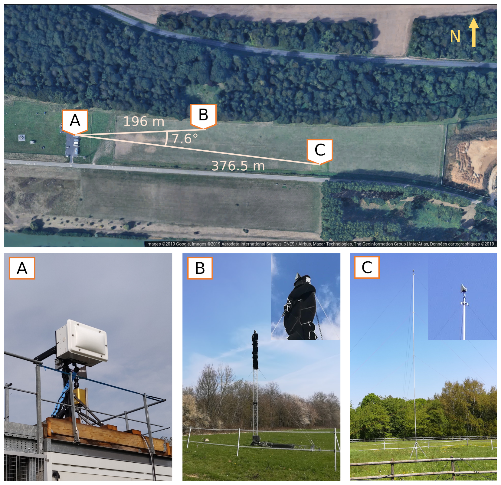
Figure 1Experimental setup for 2018 and 2019 calibration experiments. (A) Scanning BASTA mini radar located on a reinforced platform 5 m above the ground. (B) A 10 m mast with a 10 cm triangular trihedral target mounted on a pan-tilt motor with an angular resolution and repeatability better than 0.1 ∘. This mast has microwave-absorbing material wrapped around it to reduce its radar cross section (RCS; clutter). The 10 m mast was only installed in the 2019 calibration campaign. (C) A 20 m mast with a 20 cm triangular trihedral target. The target aiming is fixed relative to the mast. This mast was used in both 2018 and 2019 calibration campaigns. Angular separation between the masts is enough to sample both targets without mutual interference.
The instrument used for the calibration experiments is a BASTA mini radar. The BASTA mini is a 95 GHz FMCW radar with scanning capabilities and two parallel Cassegrain antennas (Delanoë et al., 2016). The antennas are separated by 35 cm and have a Fraunhofer far-field distance of ≈50 m, with a Gaussian-shaped main lobe (verified experimentally in Sect. 5.2). Transmitted power is fixed to 500 mW and is under constant monitoring, using a diode with an uncertainty of ≈0.4 dB. The diode enables the monitoring of Lt(T) variations, yet our experiments have shown that T is a better indicator for capturing the variability in CΓ(T,Fb). This is likely because internal temperature changes affect both Lr(T,Fb) and Lt(T) simultaneously, and therefore, the information provided by the diode is not sufficient for capturing the behavior of the whole system. The results of the temperature dependency study for our radar are shown in Sect. 5.4.
This radar also includes hardware to enable the tuning of the carrier wave frequency within a range of ≈1 GHz, centered at 95 GHz. During the experiments, we fixed the BASTA mini base frequency at 95.64 GHz to avoid any interference with the other two W-band radars operating in parallel at the same site.
Our reference targets are two triangular trihedral reflectors (also known as corner reflectors) composed of three orthogonal triangular conducting plates. Trihedral targets have a large RCS for their size and a low angular variability in RCS around their boresight (Atlas, 2002; Brock and Doerry, 2009; Chandrasekar et al., 2015). One reflector has a size parameter of 10 cm, with a maximum theoretical RCS at our radar operation frequency of 16.30 dBsm. The other is 20 cm, with a maximum theoretical RCS of 28.34 dBsm (Brooker, 2006). These targets were mounted on top of masts B and C in Fig. 1, respectively. Only mast C was used in the 2018 campaign, while both were used in 2019.
To align the system, first, we aim the radar towards the approximate position of the target. Second, we aim the target by slowly changing the pan-tilt angles in the motor on mast B or axially rotating the tube of mast C to maximize the power Pr(r0) measured at the radar. Third, radar aiming is tuned around the target position until the maximum reflected power is found. Finally, we repeat the second step, after which we have the system ready to sample Pr(r0).
It must be mentioned that this procedure does not guarantee a perfect alignment. In fact, it is impossible to have every element perfectly adjusted because of limits in the radar scanner resolution or uncertainties introduced when installing each element. Sections 4 and 5.6 explain how we deal with these limitations.
This section describes the procedure followed when performing calibration experiments using the setup described in Sect. 3. The methodology has the objective of quantifying and correcting, when possible, all sources of uncertainty to enable a reliable estimation of the calibration terms CΓ(T,Fb) and CZ(T,Fb).
A challenge we found when using targets mounted on masts to estimate CΓ(T,Fb) is that the value of the target RCS Γ0 may vary, depending on how components are aligned. Our studies have shown that, for the feasible alignment accuracy we can obtain when installing our setup, this effect is of the order of tenths of a decibel and therefore not negligible. Additionally, we concluded that, if we leave this uncertainty source uncorrected, we would introduce a bias in the calibration result (see Sect. 5.6).
The flow chart of Fig. 2 illustrates the calibration procedure. To quantify the bias introduced by alignment uncertainty, we decided to divide each calibration experiment into N iterations. Each iteration consists of a system realignment, followed by sampling of the target signal Pr(r0) for at least 1 h. Then, we select the data from the contiguous hour with the lowest variability as the iteration result.
The period chosen to perform the sampling is important because it will have an incidence on how stable the calibration value is. To minimize uncertainty, it is recommended that calibration iterations are performed when the atmosphere is clear, there is no rain and wind speed is under 1 m s−1. However, these requirements may change, depending on how robust is each setup to atmospheric conditions.
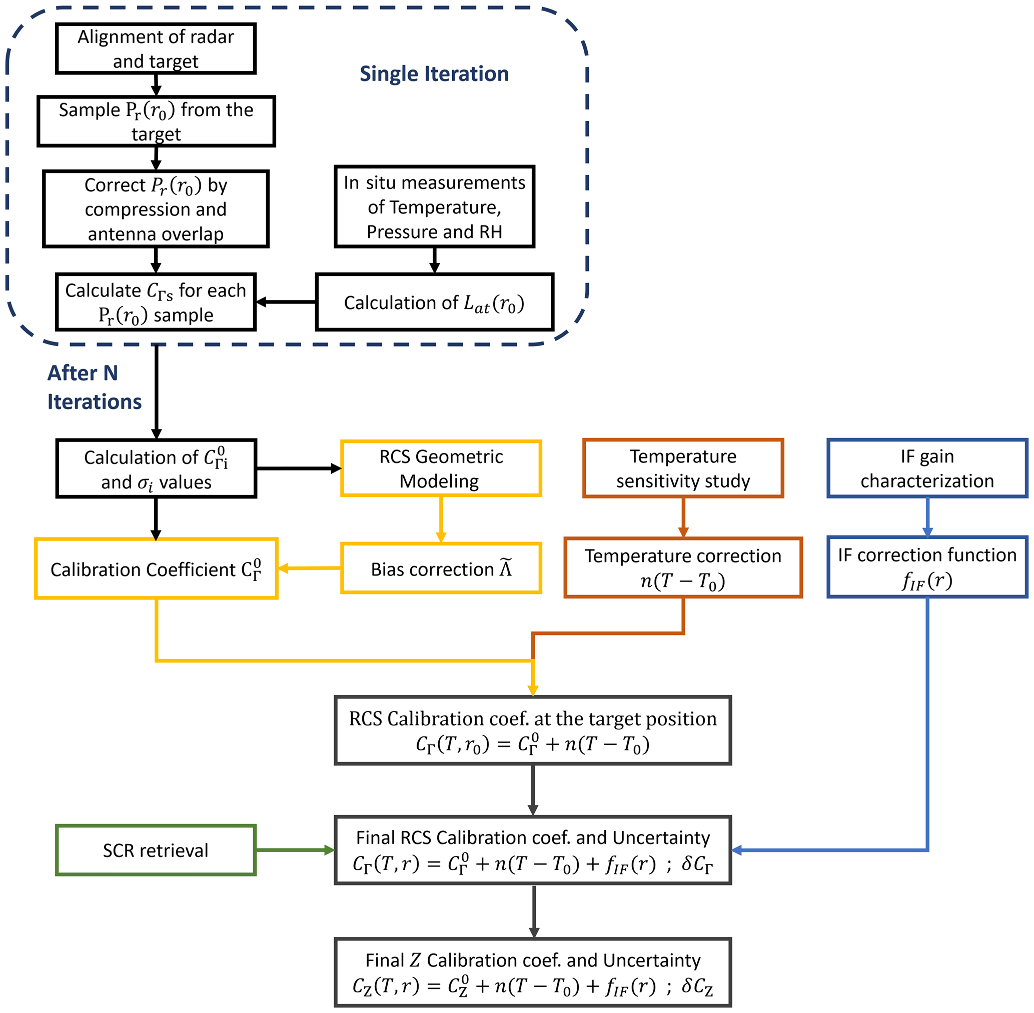
Figure 2Summary of a complete calibration process. Each calibration requires the repetition of system realignment and sampling steps called iterations. During each iteration, we continuously sample the power reflected from the reference target position for 1 h (power corrections in Sect. 5.1). The retrieval of N iterations enables the estimation of the system bias due to misalignments in the setup (Sect. 5.6). Temperature dependency is retrieved in an independent experiment (Sect. 5.4). Uncertainty introduced by clutter signals at the target location is also included in the total uncertainty budget (Sect. 5.3).
FMCW radars have a discrete distance resolution. Consequently, power measurements vs. distance are resolved in finite discrete points usually named gates. Because of this resolution limitation, the power received from a point target is spread between the gates closer to its position (Doviak and Zrnić, 2006). This phenomena is known as spectral leakage. To reduce leakage, BASTA mini uses a Hann time window (Richardson, 1978; Delanoë et al., 2016).
To correctly assess the total reflected power, we set the radar resolution to 12.5 m (chirp bandwidth of 12 MHz) and its integration time to 0.5 s. This resolution is high enough to accurately identify the reference reflector signal while avoiding the introduction of additional clutter from the trees located behind the mast (see Fig. 3).
To calculate Pr(r0), we add five gates, namely the target gate plus two before and two after the target position. Adding more contiguous gates increases the power value by less than 0.01 dB; thus, we conclude that these five gates concentrate almost all the power reflected back from the target.
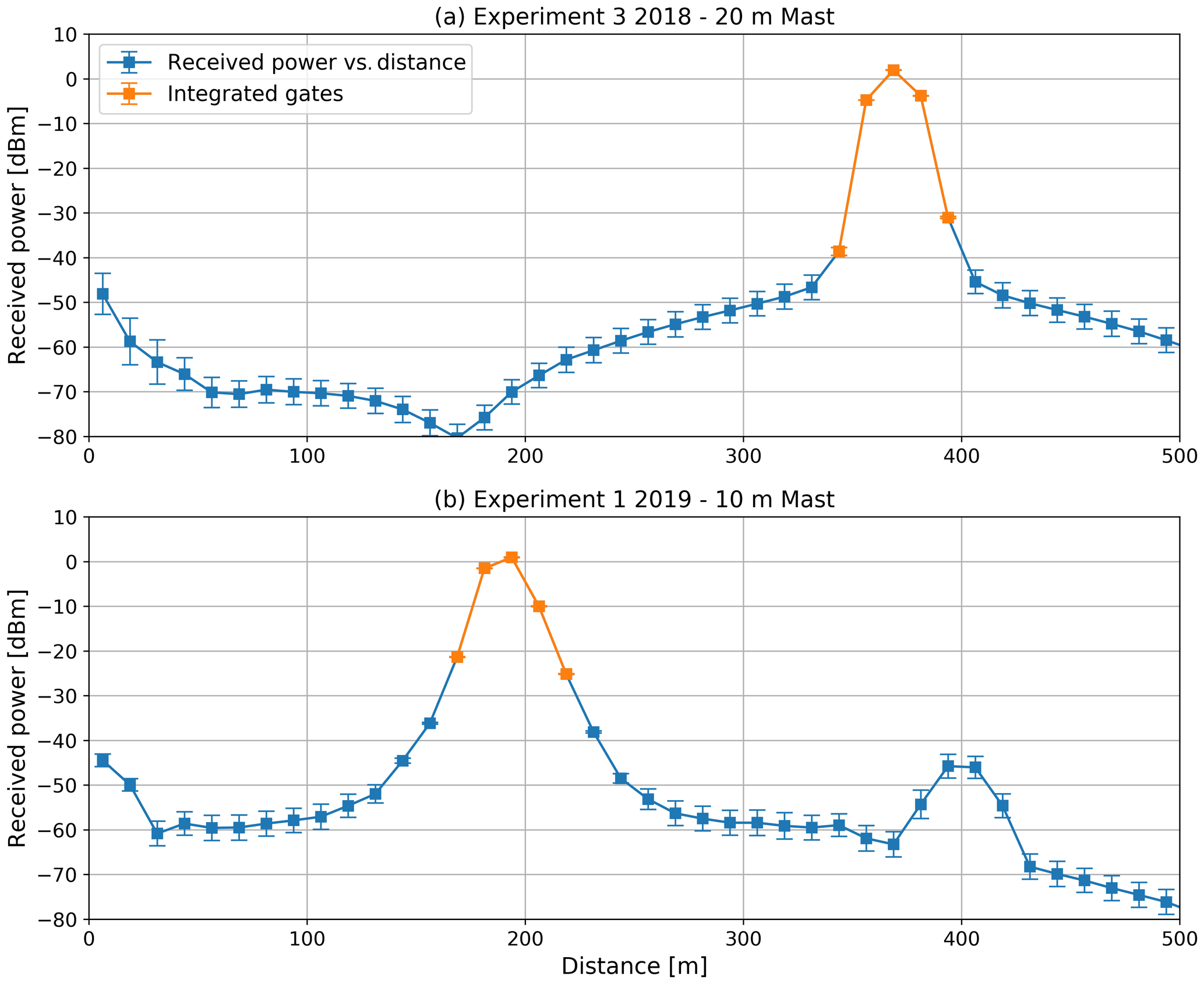
Figure 3Mean profiles of received power for experiment 5 in 2018, using the 20 m mast (a), and experiment 1 in 2019, using the 10 m mast (b). Standard deviation at each gate is indicated with an error bar. The gates are integrated to calculate the reference reflector, and the backscattered power Pr(r0) is marked in orange. The secondary peak of panel (b), around 400 m, corresponds to reflections on trees behind the 10 m mast.
Then Pr(r0) is corrected considering compression effects and antenna overlap losses (Sect. 5.1 and 5.2). For each corrected Pr(r0) sample, we proceed to calculate a single value with Eq. (4a) and the temperature correction function. This single sample is defined as to differentiate it from the final calibration coefficient of Eq. (3). Atmospheric attenuation Lat(r0) is calculated using in situ atmospheric observations and the model published by Liebe (1989).
The target-effective RCS Γ0 is calculated using a theoretical RCS model, considering the beam incidence angle on the target. Echo chamber measurements have shown that real targets of RCS can be deviated from the theoretical value, depending on the manufacturing precision. Our corner reflectors have an angular manufacturing precision better than 0.1∘; therefore, real RCS uncertainty with respect to the model can be roughly estimated to be approximately 2 dB (Garthwaite et al., 2015). Once an experimental characterization of the target becomes available, it can be used to correct any calibration bias and to reduce uncertainty by rectifying the value of Γ0 used in the calculations.
We performed one calibration experiment with six iterations during the 2018 campaign using the 20 m mast. In the 2019 campaign, we did two experiments, namely one with 10 iterations, using the 10 m mast, and another with two iterations on the 20 m mast (Fig. 1).
The retrieval of the temperature dependency coefficient n and the reference temperature T0 is done simultaneously with the calibration coefficient experiment by extending the sampling period beyond 1 h when using the 20 m mast. This is done to capture the temperature effect in the variability in by capturing a larger part of the temperature daily cycle. The results of this experiment can be seen in Sect. 5.4. Likewise, the retrieval of the IF correction function fIF(Fb) is an independent experiment based on sampling noise with the radar to obtain the IF amplification curve of the receiver. The details of this experiment are in Sect. 5.5.
From each iteration, we obtain a distribution of resulting values with a small spread introduced by second-order effects. The average value of each iteration i is named , and its corresponding standard deviation is named σi. With this information, we proceed to calculate the bias-corrected calibration coefficient by using Eq. (6). is the bias-correction term. The method used to calculate λ relies on simulating the probability distribution of Γ0 for a given set of uncertainties in the setup parameters. More detail can be found in Sects. 5.6 and S3 in the Supplement.
Equations (7a) and (7b) show the uncertainties δCΓ and δCZ associated with the estimation of CΓ(T,Fb) and CZ(T,Fb), respectively.
σT is the uncertainty term associated with the temperature correction function n(T−T0).
σIF is the uncertainty term associated with the IF loss correction function fIF(Fb).
The term comes from the averaging operation in the estimation of (Eq. 6). Since the terms are corrected using the temperature correction function, the uncertainty of the latter must be propagated as well; hence, the term appears.
σΛ is the uncertainty of the bias correction calculation. It is calculated from the standard deviation σi. This procedure is explained in Sect. S3.
σSCR is the uncertainty introduced by clutter. Clutter is the presence of unwanted echoes, which affect our reading of Pr(r0), coming from reflections on other objects in the environment. The method of quantifying the uncertainty σSCR uses a parameter named signal-to-clutter ratio (SCR), which is explained in detail in Sect. 5.3.
is the uncertainty of the reference target RCS. In this work, we use a theoretical model to calculate the target-effective RCS, which has an uncertainty of approximately 2 dB based on the manufacturing characteristics. The inclusion of an experimental characterization of the target RCS can improve the estimation of and δCΓ by reducing this uncertainty term.
σK is the uncertainty in the estimation of the backscattering particles dielectric factor. Because our objective is to calculate the calibration term of the radar, we reference this value to , corresponding to pure water at 5 ∘C, and neglect the δK uncertainty term. However, the value of K and its uncertainty σK must be considered when performing radar retrievals (e.g., Sassen, 1987; Liebe et al., 1989; Gaussiat et al., 2003).
σA is the uncertainty introduced in the estimation of θ and from parallax errors and deviations from a Gaussian beam shape (Sekelsky and Clothiaux, 2002). For this work, we make the assumption of parallel antennas with a Gaussian beam shape; thus, we neglect this term. This problem is discussed more in depth in Sect. 5.2.
Since both σK and σA are neglected, we obtain δCΓ≈δCZ.
In this section, we identify and quantify the uncertainty and bias introduced by several terms in Eq. (2b). Following the recommendations in the work of Chandrasekar et al. (2015), we study the impact of receiver saturation, signal-to-clutter ratio, antenna lobe shape and antenna overlap. Additionally, we consider the impact of temperature fluctuations inside the radar box, loss changes with distance due to uneven amplification at the receiver's IF and the effects of imperfect alignment of the reference target.
5.1 Receiver compression
It is advisable to design calibration experiments which avoid the appearance of compression effects. If this is not possible, compression must be considered in the data treatment so that the retrieved calibration remains valid in the receiver linear regime, where it usually operates during cloud sampling (Scolnik, 2000).
To study how these effects could affect our calibration, we retrieved the radar receiver power transfer curve. Receiver characterization was done by removing the radar antennas and connecting the emitter end to the receiver input with two attenuators in between. The first was a 40 dB fixed attenuator, while the second was a tunable attenuator covering the range between 50 and 1 dB of losses. The adjustable attenuator enabled the retrieval of the power transfer curve by varying the attenuation and sampling the power at the receiver end (digital processing included). Our retrieved power transfer curve is shown in Fig. 4a.
Compression effects must be considered in calibration, or a bias will be introduced. As a consequence, we include compression correction in every sample of reflected power, which consists of projecting their value to the ideal linear response using the power transfer curve.
For example, the power received from the 20 cm target on the 20 m mast returned was 4.1 dBm, on average, before corrections. The power transfer curve shows that, at this power value, we have a loss caused by a compression of ≈0.3 dB. After correcting each power sample by compression with the power transfer curve, we obtain a corrected power average value of 4.5 dBm. Meanwhile, for the 10 cm target on the 10 m mast, the average power value before corrections is 3.2 dBm. As this value is lower than what is obtained by the 20 m mast, the associated compression effect is also smaller at ≈0.2 dB. After applying this correction to each power sample, we end with a new, corrected power average of 3.4 dBm.
5.2 Antenna properties
Manufacturer specifications indicate that antenna beamwidth should be 0.8∘. However, data from an experimental characterization done by the same manufacturer in an anechoic chamber indicate that antenna beam shape is better approximated by a Gaussian function with a half-power beam width (HPBW) of θ≈0.88∘. The integrated gain difference between the experimentally retrieved curve and the Gaussian function is of ≈0.0003 dB in the HPBW region. Therefore, we conclude that the contribution to uncertainty introduced by assuming a Gaussian beam shape is negligible. The antenna beam shape and Gaussian curve are shown in Fig. 4b.
Another source of bias introduced by the antennas is the parallax error. Antenna parallax errors introduce a range-dependent bias determined by the antenna beamwidth and the relative angles of deviation between the antennas' boresight. This bias is usually larger in the first few 100 m closest to the radar. For example, for a deviation of half of the antenna beamwidth, losses would be of the order of 10 dB and would vary significantly over the first hundreds of meters, decreasing with distance to about 1 dB at a approximately 4 km (Sekelsky and Clothiaux, 2002).
To study this effect, we took advantage of our experimental setup and the scanning capabilities of the radar to check if the radar antennas were properly aligned. This was done by using the target on the 20 m mast. Results are shown in Fig. 4b. After analyzing the results, we observed that the aiming uncertainty is of the same order of magnitude as the antennas' beamwidth. Since the correction of the parallax error requires a very precise measurement of antenna alignment, we conclude that it is not possible to directly correct for antenna deviations with this information.
However, the relatively small difference of 0.5 dB in the estimation of during the calibration experiments of 2019, obtained using two masts in the most sensitive distance range (placed at a distance of 196 and 376.5 m, respectively), indicate that antennas are unlikely to have a deviation comparable to their beamwidth (calibration results in Sect. 6).
Therefore, for the present version of this calibration methodology, we assume that both antennas are parallel and that they have a Gaussian beam lobe. Once a reliable method for antenna pattern retrieval is developed for W-band radars, it can be directly incorporated into the calibration term by adding an additional correction function fA(r) to Eq. (3). The uncertainty in this alignment estimation can also be included in the uncertainty budget with the term σA of Eq. (7b).
Even if the antennas are parallel, it is necessary to include a correction for the loss Lo(r) caused by incomplete antenna overlap. The correction, shown in Eq. (8), accounts for the loss in power that would be received from a point target compared to a monostatic system (Sekelsky and Clothiaux, 2002). This loss occurs because a point target cannot be in the center of two nonconcentric parallel antenna beams.
Equation (8) assumes that the radar has two identical, parallel antennas with Gaussian beam lobes. Their main axis is separated by a distance d, and the point target is located at a distance r, facing the geometrical center of the radar, where the gain is maximum. The antenna separation d of BASTA mini is of 35 cm, introducing a loss of 0.08 dB for the target at r0=196 m and of 0.02 dB for the target at r0=376.5 m.
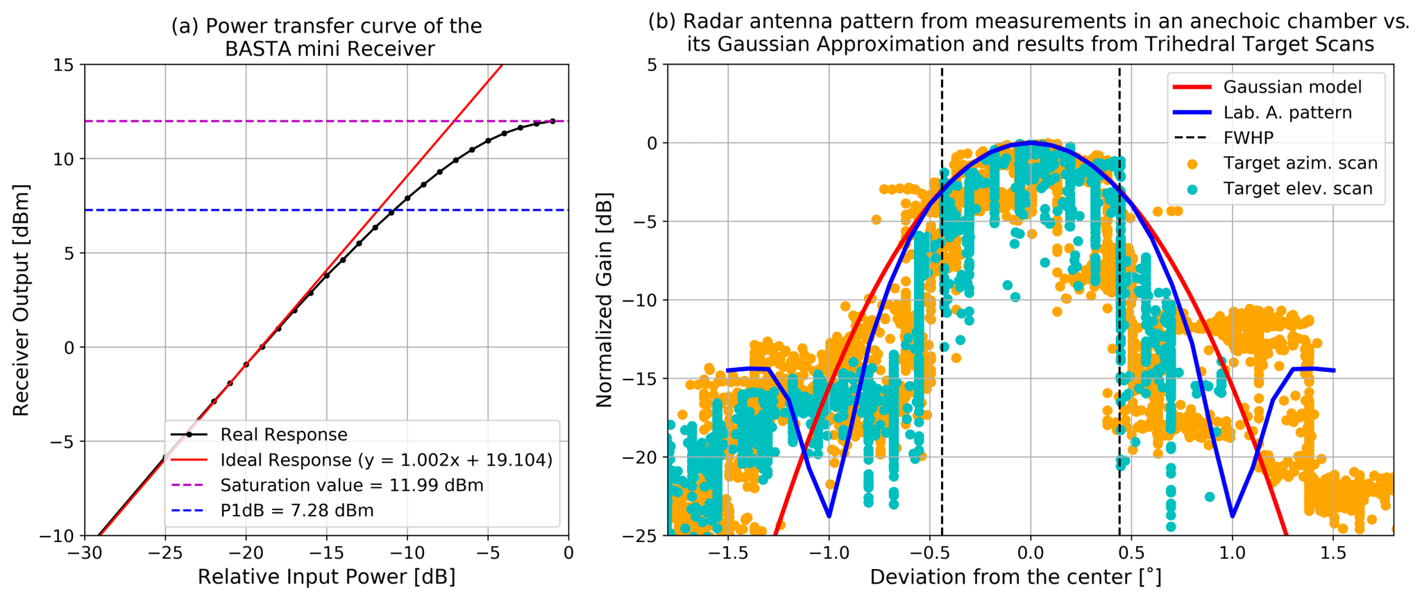
Figure 4(a) Power transfer curve of the BASTA mini receiver. Input power is relative to the minimum attenuation value of the curve characterization experiment. All our signal retrievals from the target are slightly under the 5 dBm line; thus, the correction required due to compression effects is small (<0.3 dB). (b) Normalized antenna pattern of the BASTA mini antennas. We can observe that the Gaussian fit with a beamwidth of θ=0.88∘ is very close to the antenna gain curve measured at the manufacturer's laboratories. This figure also shows the results from mast scans around the target for comparison with the theoretical curves. To enable the comparison with the laboratory antenna pattern, we assume that the gain of both antennas is identical. Then, the received power in decibels per milliwatt is normalized with respect to the maximum measured value and divided by two to represent the gain of a single antenna.
5.3 Signal-to-clutter ratio
The power sampled from our reference reflector is an addition of the power from the target (signal) and unwanted reflections on other elements in the environment, such as the ground or the mast (clutter). We observed that this clutter dominates above the radar noise, and thus becomes the main source of interference in our calibration signal.
To quantify the impact of clutter, we use the signal-to-clutter ratio (SCR) parameter. It is calculated as the ratio of total power received from the target to the power received from clutter under the same configuration but with the reference reflector removed. SCR enables the uncertainty σSCR introduced by clutter in the sampled Pr(r0) values to be computed (Chandrasekar et al., 2015).
Clutter power is sampled and corrected following the same methodology used for reflector Pr(r0) retrievals but in an scanning pattern mode to capture clutter around the mast area. Figure 5 shows our results from scanning around the 10 and 20 m masts with the targets removed.
We observe that the 10 m mast is more reflective than the 20 m one. This may be caused by its smaller height (more ground clutter) and its larger geometrical cross section. We can also see that the signal at the 10 m mast is stronger where absorbing material is not present (below ≈1.5∘ of elevation). In both cases, we did not detect any signal from the nearby trees close to the target position.

Figure 5Clutter retrieval from the 10 m (a) and 20 m masts (b), respectively. Masts are scanned without the reflectors to measure the clutter signal. The nominal target position is marked with a black cross.
To calculate SCR, we compare the average power received from each target during the calibration experiments with the maximum clutter power observed in a region of 0.125∘ around the target coordinates, both vertically and horizontally. The value is taken from the radar scanner resolution.
The average power received from the 10 cm target on the 10 m mast is 3.4 dBm. This provides an SCR value of 19.4 dB, which implies a σSCR uncertainty value of ≈0.93 dB. From the 20 cm target on the 20 m mast, the average received power is 4.5 dBm. Its SCR equals 40.1 dB, which is translated as an uncertainty contribution of σSCR≈0.09 dB. From the results, we see that even if target alignment is better with the 10 m mast, calibration results may not be less uncertain because the motor used for target alignment acts as a big source of clutter.
5.4 Temperature correction
BASTA mini has a regulation system to control temperature fluctuations inside the radar box. However, since the radar is based on solid-state components, even small temperature fluctuations may impact the performance of the transmitter and receiver and, therefore, affect the calibration stability. To account for this effect, we introduced a temperature dependency in the calibration term, as shown in Eq. (3).
During the experiments, we verified the need for this correction by observing that the retrieved calibration term CΓ(T,F0) has a consistent change, depending on the time of the day, and that this change is strongly correlated to the temperature inside the radar.
Figure 6a, b and c show the results of a representative experiment done in the 2018 campaign. Here we left the radar sampling the target signal for several hours to observe the variability in CΓ(T,F0) during the day. Figure 6a shows the raw result in the RCS calibration term CΓ(T,F0). There is a spread of almost 1 dB between the maximum and minimum values during the whole time series. Figure 6b is a Fourier transform of this raw time series. Here we can see that most of the variability happens in the timescale of hours. Figure 6c presents the time series of Fig. 6a but in a daily cycle perspective. Here we plot hourly means of the deviation of CΓ(T,F0), with respect to the total average, with its hourly standard deviation as error bars. We also superimposed the atmospheric attenuation and the radar amplifier temperature to show that the former has a much smaller impact in calibration variability compared to the latter.
Figure 6d shows the raw results of plotting variations in CΓ(T,F0) to temperature changes around T0=26.5 ∘C. These variations are calculated independently for each iteration by subtracting the constant term of the linear fit of CΓ(T,F0) with respect to temperature. This operation removes the effect introduced by differences in alignment between the different iterations. The reference T0 value is chosen because it is approximately the average internal temperature when considering all the experiments.
To maximize the range of temperatures covered, we choose to not limit the sampling period to 1 h. This decision has the drawback of increasing the noise of the data set due to the inclusion of some data taken under suboptimal conditions, for example, with wind speed velocities above 1 m s−1 or with the presence of drizzle. Yet, this step is necessary to enable the retrieval of the temperature correction function for the widest range of temperatures possible.
To retrieve the temperature dependency, we perform a linear regression over the results from all the experiments done in 2018 and 2019, as shown in Fig. 7. The regression shows that the variability in the calibration term has an almost-linear relationship with the internal radar temperature, in the decibel scale, and it is the same for both campaigns. This analysis allows us to estimate the value n=0.093 dB ∘C−1 for the temperature correction function of Eq. (3). To estimate the uncertainty of the temperature correction function, we calculate the root mean square error (RMSE) between the linear regression model and the whole data set for each degree of deviation in temperature. The RMSE value for the complete data set is of 0.13 dB, while its value per degree ranges between 0.07 and 0.23 dB for a deviation of 0 and +3 ∘C, respectively. These results enable us to conclude that the temperature correction function uncertainty σT is ≤0.23 dB.
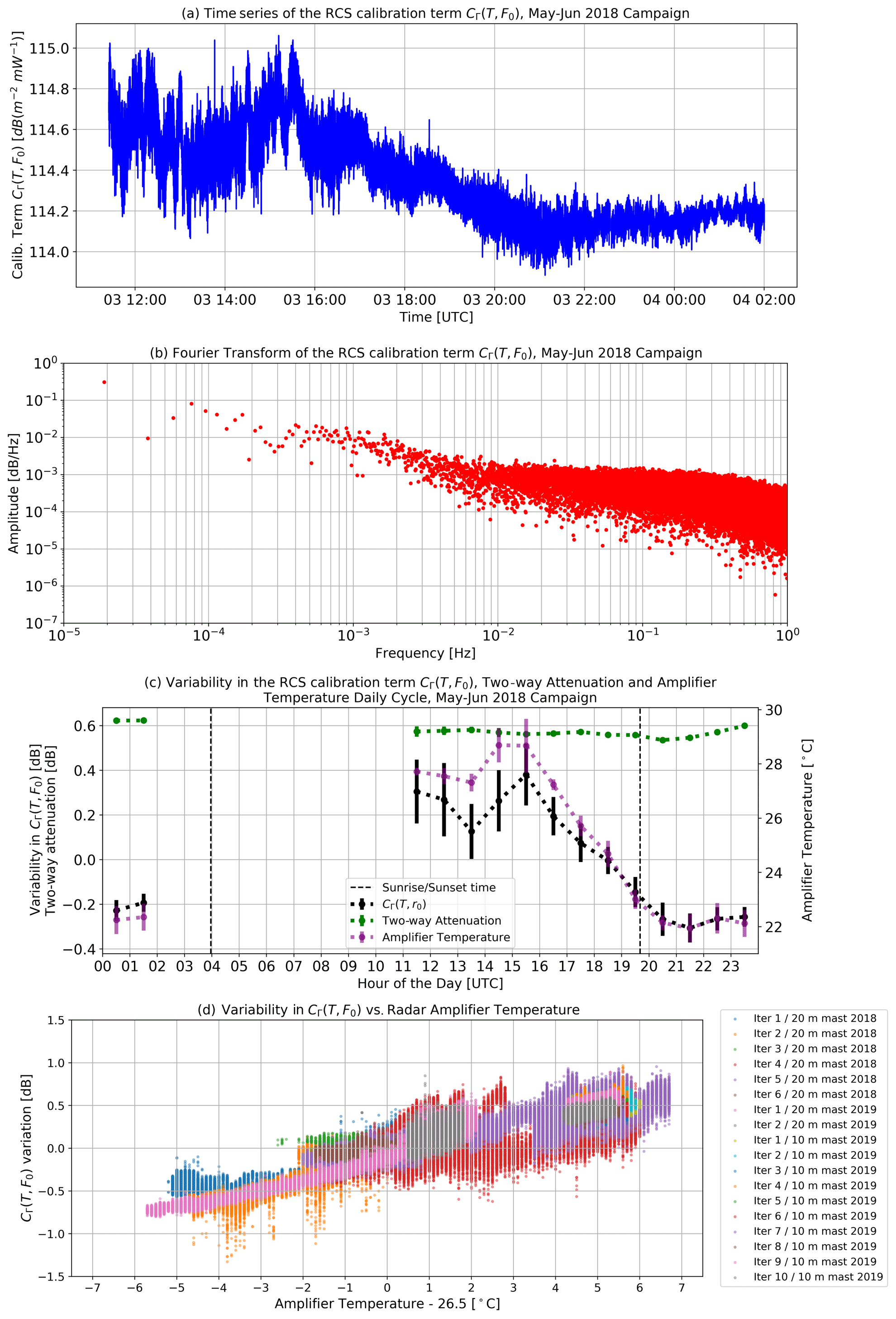
Figure 6Calibration variability study. Samples from iteration 5 of the 2018 calibration campaign. (a) Time series of the RCS calibration term retrieval. (b) Fourier transform of the RCS calibration term after subtracting the mean value. (c) Calibration variability daily cycle, amplifier temperature and two-way attenuation. Attenuation error bars are too small to be seen at this scale. (d) Relative changes in CΓ(T,F0) versus amplifier temperature plotted using all samples from the 2018 and 2019 campaigns.
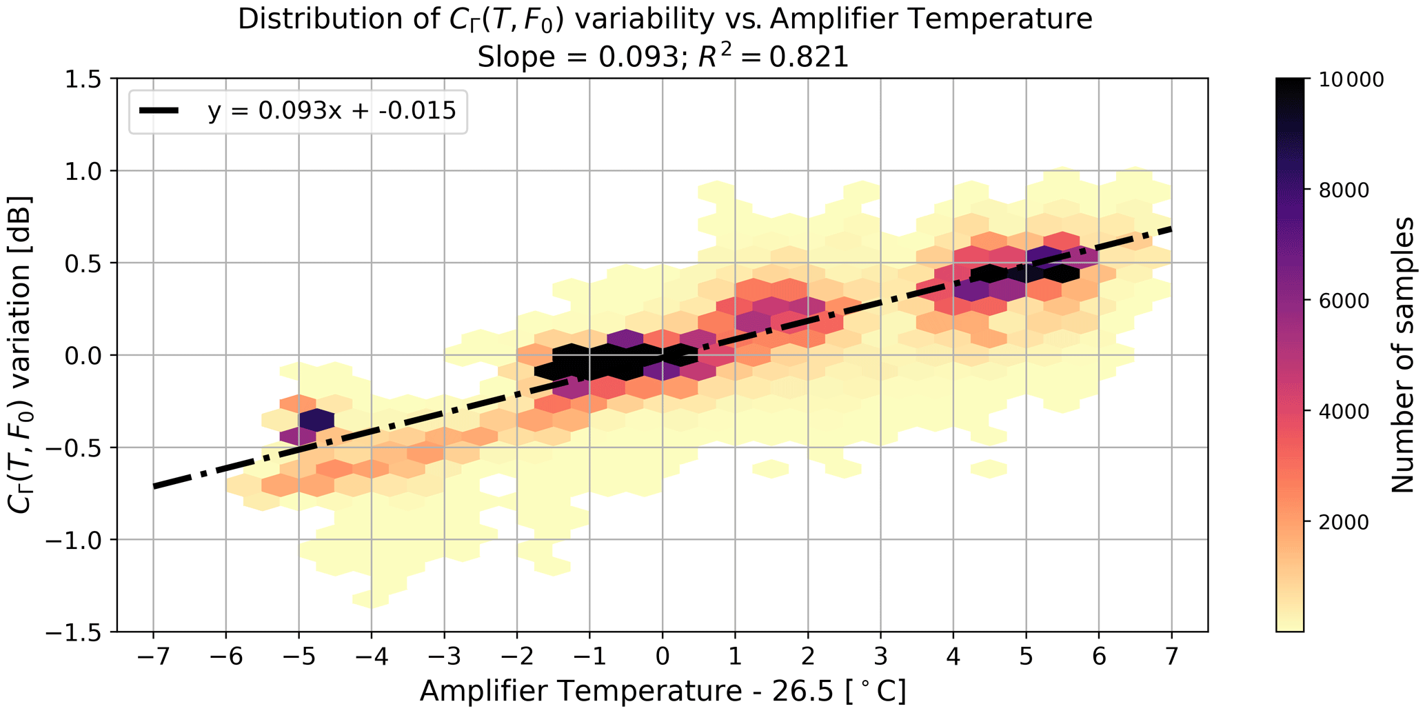
Figure 7A 2D histogram of the relative changes in CΓ(T,F0) with respect to changes in the amplifier temperature and its linear least squares fit. The histogram is plotted using all CΓ(T,F0) samples from the 2018 and 2019 calibration campaigns.
5.5 IF loss correction function fIF(Fb)
FMCW radars rely on estimating the beat frequency of the received signal to estimate the distance of an object. This signal may suffer uneven amplification, depending on its frequency, because of a frequency-dependent gain function in the amplifiers of the IF chain of the radar. Since there is a direct relationship between the IF frequency Fb and the target distance r, this dependency on the beat frequency introduces a gain variability with respect to the target distance r. As introduced in Sect. 2, this distance dependency is compensated in the calibration term with a IF correction function fIF(Fb).
The power Pr(r) measured by the receiver when no active signal is inputted corresponds to the system noise power Ns(Fb) plus the environmental noise power N0 amplified by the radar receiver gain Gr(T,Fb) (this gain term is equivalent to of Eq. 2a). Equation (9a) expresses this relationship when Pr(r) is in decibel milliwatts and N0 and Ns(Fb) are expressed in linear units (Pozar, 2009).
The standard way to retrieve each of these terms is to perform a two-point calibration. This requires the use of two noise sources at significantly different and well-known temperatures. Usually, the temperatures of the noise sources are the environmental temperature (298 K) and that of liquid nitrogen (77 K) (Rodríguez Olivos, 2015). The receiver gain versus the frequency retrieved from this two-point calibration could be used to derive the IF correction function directly. However, this approach requires tailored equipment which was not available during the experimentation. Therefore, since the IF correction function is important for removing calibration bias, we follow a different approach when estimating its value.
To estimate the IF correction function, we take advantage of the narrow IF bandwidth of the BASTA mini radar (12 MHz, from 168 to 180 MHz). A calculation done with the Friis formula for the radar system indicates that the system noise Ns(Fb) should have variations smaller than 0.1 dB in this bandwidth. This can be explained by the large operating bandwidth and the high gain of the receiver low noise amplifier (LNA) of 35 GHz and >20 dB, respectively, and by the small variation in the mixer conversion loss for the radar bandwidth (<0.3 dB). To verify the plausibility in the estimation of the noise figure variability, we performed an additional calculation testing the effect of varying the IF noise temperature from 0 to 400 K, and in all cases, the system noise variability remained under 0.1 dB.
This low variability enables the retrieval of the IF correction function by assuming a constant noise power density in the IF frequency range (Eq. 9b). The constant noise power term Nc corresponds to the addition of environmental and system noise.
Then, to retrieve the fIF(Fb), we turn off the radar emitter and sample the environmental noise with the radar operating in its calibration configuration (12.5 m distance resolution and 0.5 s integration time). After retrieving a significant amount of noise samples, we calculate the average value of the difference Pr(F0)−Pr(Fb) for each IF frequency Fb to remove the effect of the unknown noise power density. This operation is done to quantify relative gain variations around the calibrated frequency F0.
By using Eqs. (2a) and (3), we find that the difference Pr(F0)−Pr(Fb) is equivalent to the difference between CΓ(T,Fb) and CΓ(T,F0), and therefore, it is equivalent to the IF correction function fIF(Fb) (Eq. 10). The temperature effect in gain is removed because both Pr(F0) and Pr(Fb) are sampled simultaneously and, therefore, under the same temperature conditions.
For this experiment only, Pr(F0) corresponds to the power measured at the gate closer to the reference target position without integrating other gates. This is done because there is no significant leakage and, as the results in Fig. 8 show, Gr(T,Fb) changes are negligible in the five gates used for integration.
Figure 8 shows the results of the IF correction function retrieval referenced to Pr(F0), using F0 associated to the target distance r0=376.5 m (corresponding to the 20 m mast experimental setup). We can observe that all functions retrieved in 2019 are in close agreement, without significant variations between different dates or times of the day chosen for the plots. The 2018 function is different because the hardware was modified between both calibration campaigns. Additionally, in 2018 the emitter was not turned off to perform the noise sampling. Rather, we resorted to using a sampling period with clear-sky conditions to respect the assumptions of Eq. (9b). To avoid the effect of crosstalk, we only consider gates farther than 200 m from the radar.
A sixth degree polynomial is used to fit fIF(Fb). For both 2018 and all 2019 curves, the fit has a RMSE <0.03 dB. Furthermore, the standard deviation between the results from the four periods of 2019 has a maximum value of 0.04 dB for any gate. Both results indicate that the uncertainty introduced by the IF correction function is ≤0.04 dB. Finally, the IF correction function retrieved for the 10 m mast setup in 2019 (with r0=196 m) is almost identical to the 20 m mast results. These functions are presented in Sect. 6. Considering these low RMSE values, we decided to select the uncertainty introduced by assuming a constant system noise as the IF correction function uncertainty; thus, σIF=0.1 dB.
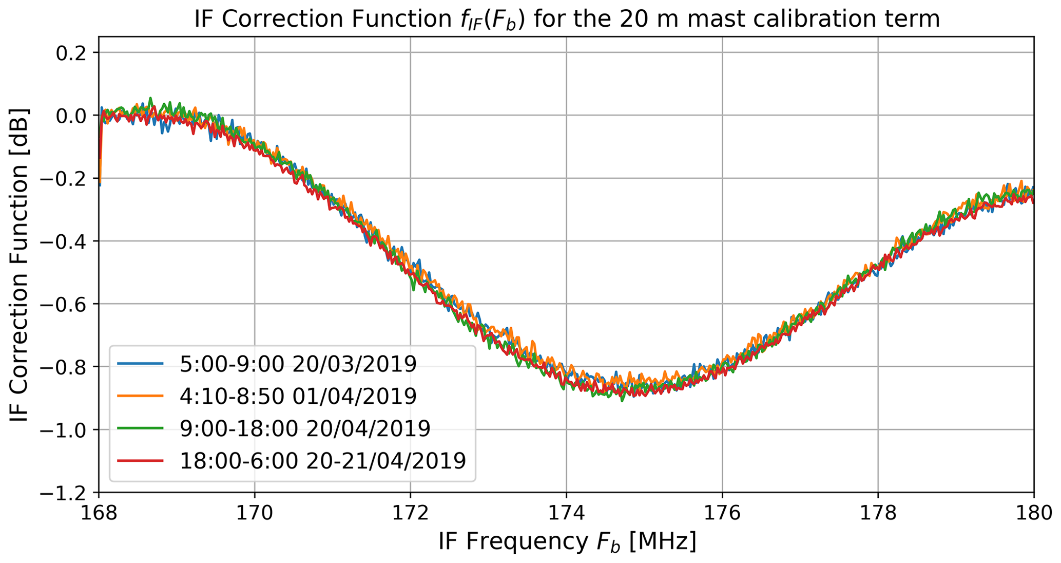
Figure 8Data used for the IF correction function calculation, retrieved for different periods of the 2019 calibration campaign. The 2018 IF correction function is different from the 2019 results because the hardware was modified between the campaigns (see 2018 IF correction function presented in Sect. 6). The time indicated in the label is in universal coordinated time (UTC).
5.6 Misalignment bias
The retrieval of CΓ(T,F0), using Eq. (4b), requires a precise knowledge of the reference target effective RCS Γ0. Each decibel per square meter of difference between the theoretical value used in the calculations and the effective target RCS will introduce a bias of the same magnitude in the estimation of the calibration coefficient and, thus, in CΓ(T,F0).
The effective reflector RCS is the actual physical value that would be measured by a perfectly calibrated radar. It is different from the target-intrinsic RCS which only depends on its physical properties. Effective RCS changes when the experimental setup is modified. For example, if the point target is not exactly in the beam center, the antenna gain will not be maximum, and therefore, the effective RCS will decrease compared to the intrinsic value. Effective RCS also changes when the incidence angle of the radar beam is modified. This latter effect may increase or decrease effective RCS, depending on the original situation.
A common approach in these type of experiments is to set Γ0 to be the maximum theoretical RCS of the target, assuming misalignment will cause a negligible deviation from this value. This procedure can be refined for cases in which the system default configuration does not have the target boresight aligned with the radar position. In these cases, effective RCS can be calculated using equations derived from geometrical optics (more complex optical calculations may be necessary for other wavelengths or target sizes). For example, we use the equations published by Brock and Doerry (2009) when calculating the effective RCS of our triangular trihedral target on the 20 m mast.
Unfortunately, this approach does not correct the impact of alignment uncertainties. We observed that random errors in the element positioning will statistically impact the effective Γ0 in a single direction. Thus, simply taking the average of many target sampling iterations would result in a biased estimation of the calibration.
With the objective of quantifying the impact of alignment uncertainties, we developed a geometrical simulator of effective RCS. This simulator receives as input the position of each element in the setup and calculates the effective RCS, considering the beam incidence angle and antenna gain variations when the target is not in the center of the beam. The degrees of freedom included in the simulator are shown in Fig. 9a. It enables the modification of the radar aiming angles, the mast dimensions and the positioning and orientation of the target. The equations used in the simulator can be found in the Supplement.
We now use the simulator to study how uncertainty in alignment can affect the value of Γ0. For this, we model an example experiment based on the 20 m mast setup. In this model, we separate input variables between known and uncertain. Known terms can be fixed or measured very precisely in the field experiment; hence, they are set as fixed values. Meanwhile, uncertain terms represent the parameters that cannot be fixed or measured very precisely and, for that reason, are better expressed as probability distributions (terms defined in Fig. 9a).
-
Known terms, as follows:
- –
xr=376.5 m
- –
hr=5.3 m
- –
ρ=20 m
- –
α=48∘
- –
target size =20 cm.
- –
-
Variables with uncertainty, as follows:
- –
- –
- –
- –
- –
.
- –
In the uncertain variables, ∘, ∘ and ∘ represent the nominal alignment angles, which are the values expected under an ideal field experiment where the radar aims directly at the target and the mast is perfectly vertical. To these nominal values we associate a distribution shape and the uncertainty set of ∘, ∘, σθ=1.5∘ and στ=5∘. Each term, known and uncertain, is estimated from observations done during the experimental field work.
With these input parameters, we sample the Γ0 distribution that would arise after a large number of experimental iterations. Figure 9b shows the results from this sampling. The black dashed line shows the effective RCS under our experimental configuration when each element is in its nominal position. We can see that this effect cannot be neglected in our case since its value is 0.8 dB lower than the maximum theoretical RCS.
However, this single correction does not suffice. The results of the model show that the addition of uncertainty into the process induces another bias of ≈0.3 dB on average. Since this is within the order of magnitude of our desired uncertainty in the calibration, the example clearly illustrates the need for including a bias correction step in our calibration methodology.
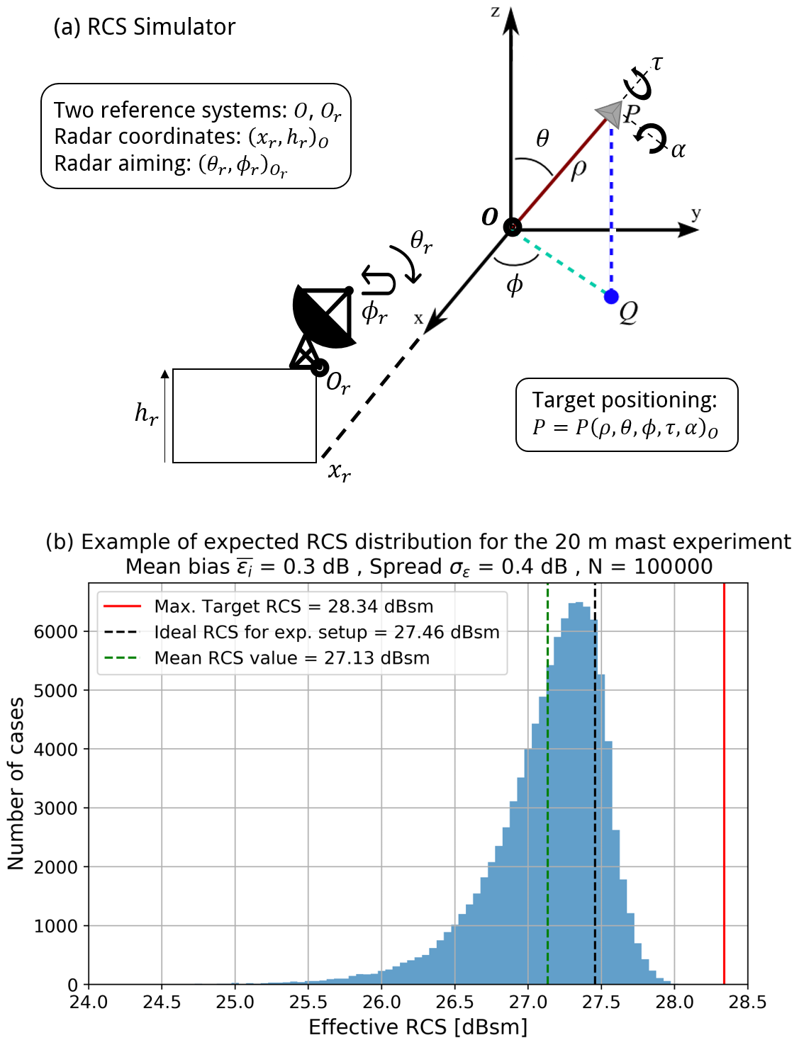
Figure 9(a) Diagram of the RCS simulator illustrating its degrees of freedom. (b) Example of an effective RCS distribution obtained after 100 000 simulations with the uncertainty set specified in the text. The simulations are based on our 20 m mast setup. Bias is calculated by subtracting the ideal RCS from the mean RCS value. The example illustrates how the effective RCS will be, statistically, lower than the result expected from an ideally aligned setup.
The standard deviation σϵ between N experimental retrievals of cannot be used directly as an estimation of uncertainty because the RCS distribution shape is not Gaussian. The uncertainty introduced by this variability is studied by sampling a large set of possible RCS distributions, based on our experimental configuration, and selecting the candidates matching our observed spread σϵ. This set provides an estimation of the expected bias correction and of the effective RCS uncertainty σΛ. The uncertainty of the estimator of Eq. (6) will correspond to the uncertainty of each estimation propagated through the calculation of their average (terms and in Eq. 7a) plus the effective RCS uncertainty σΛ. The details on how this estimator works and how the RCS distribution sampling is done are fully explained in Sect. S3.
In 2018 we used the 20 m mast only, performing six iterations. For 2019, we did 10 iterations using the 10 m mast and two iterations with the 20 m mast. The distributions of obtained in each iteration and experiment are shown in Fig. 10.
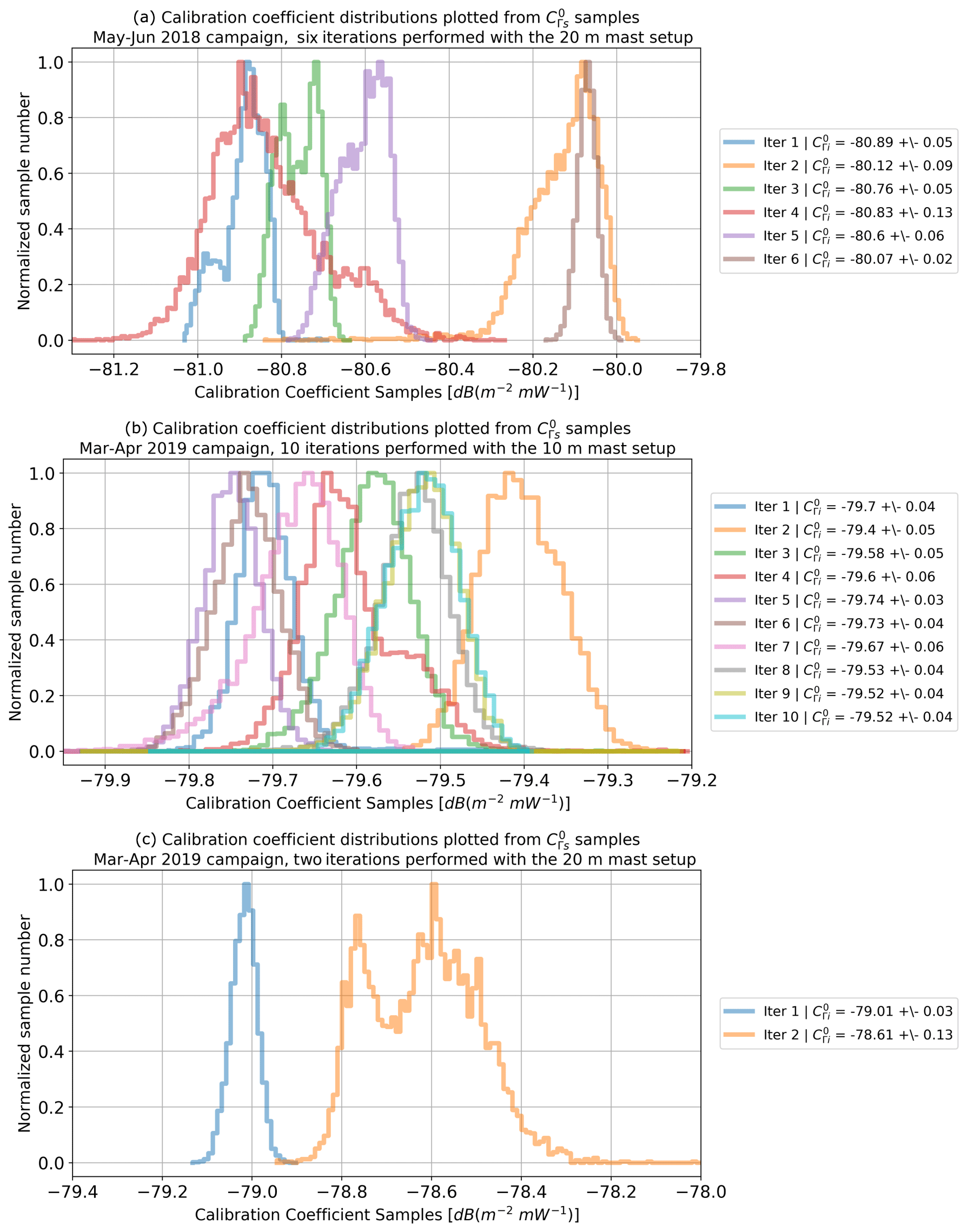
Figure 10Calibration coefficient distributions obtained for the (a) 2018 campaign using the 20 cm target on the 20 m mast, the (b) 2019 campaign using the 10 cm target on the 10 m mast and the (c) 2019 campaign with the 20 cm target on the 20 m mast.
The radar hardware changed between the 2018 and 2019 campaigns due to experiments that required retrieving the power transfer curve and performing maintenance operations. This implies that we cannot compare the absolute calibration values between both campaigns. What remains valid is the comparison of the properties, such as the variability, and the results from both experiments in 2019.
In the results, we can notice a difference in the spread when comparing the 10 and 20 m masts. The six iterations of 2018 (Fig. 10a) have a spread of σϵ=0.33 dB, while the spread of the 10 iterations of 2019 is 0.11 dB (Fig. 10b). This happens because the 10 m mast has a motor on top which enables a much finer adjustment of the target position, improving the repeatability of the experiments.
There is also a small difference in the spread of the curves. The values retrieved in experiment (B) have a smaller spread σi. This is because we took all the samples during one single night with very clear conditions and an average wind speed below 1 m s−1. A great advantage was the presence of the motor that enables target alignment in ≈5 min. Meanwhile, for experiment (A), curves were sampled during different days because the 20 m mast setup requires more time to align (≈2 h). The different conditions on each day led to a more varied shape in the retrieved curves. This effect is specially noticeable in experiment (C), where the iterations were performed during daytime when atmospheric conditions are more dynamic, especially the wind speed variability. The introduced variability was not fully compensated by our corrections and, thus, bimodal distributions remained. However, the individual spread is still small, within ≈0.1 dB, so we decided to accept these samples for calibration purposes.
Table 1Bias correction and its uncertainty σΛ calculated using a different number of iterations for the experiments of the 2018 and 2019 calibration campaigns (e.g., three iterations means we used iterations 1, 2 and 3 of the experiment). We include the average and spread σϵ between the retrieved for each case. This variability σϵ is introduced in the bias estimation procedure to determine the bias correction and its uncertainty σΛ.
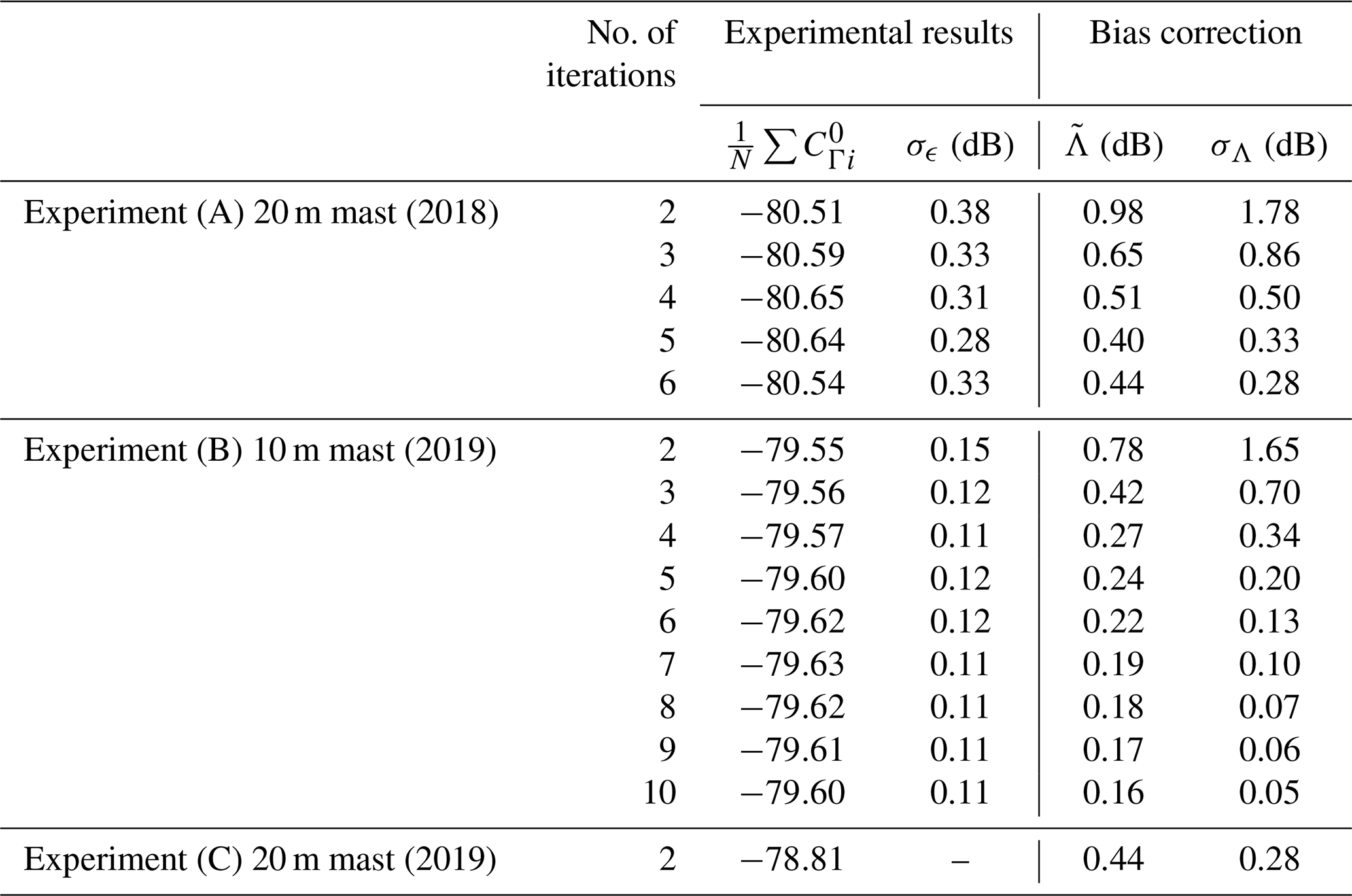
To study the dependency of the bias correction on the number of iterations, we calculate the bias correction term and its uncertainty σΛ for experiments (A) and (B) with different numbers of repetitions. The order of the iterations used in each row matches the sequential order indicated in Fig. 10. The results are shown in Table 1. For both cases we have the best estimate when we use all the samples available for each experiment, and thus, we use this bias correction and uncertainty when computing the calibration coefficient.
For experiment (C), we followed a different approach. Because we only have two samples, the calculated σϵ=0.2 dB is very likely to be underestimated. Consequently, and because the experimental procedure was identical to what was done in 2018, we assume our parameters σϵ, and σΛ to be equal to the best estimation of experiment (A). This is possible because in our methodology we assume that the bias probability distribution of a given system is unique, even if it is unknown, and what is done by performing many iterations is successively restricting the possible sets of uncertainties that can generate results consistent with the observations. This latter hypothesis is consistent with the decrease in uncertainty for the bias correction when increasing the number of iterations. Table 2 contains a summary of all known bias corrections and uncertainty contributions, as introduced in Sect. 4. With the aforementioned results, we use Eqs. (6), (3), (7a) and (7b) to estimate the RCS and reflectivity calibration terms CΓ(T,Fb) and CZ(T,Fb) alongside their uncertainty. Since the term is much larger than all other uncertainty sources, we calculate a partial calibration uncertainty including all but this term to simplify the comparison of uncertainty contributions between different experimental setups. This term is then added for the calculation of the final result. CZ(T,Fb) is calculated for the range resolution δr=12.5 m, which is the same mode used for target sampling. T is the radar amplifier temperature in degrees Celsius and fIF(Fb) is the IF loss correction function.
-
Experiment (A), 20 m mast (2018):
- –
- –
- –
.
- –
-
Experiment (B), 10 m mast (2019):
- –
- –
- –
.
- –
-
Experiment (C), 20 m mast (2019):
- –
- –
- –
.
- –
Table 2Summary of all known corrections and uncertainty contributions in the calculation of CΓ(T,Fb). The absolute correction terms have a sign associated with the direction in which they impact the final calibration calculation. For the receiver compression correction, we present the average magnitude, and for the temperature correction, we present the range of possible values. The partial calibration uncertainty is the addition of all uncertainty terms except . This term is later added to calculate the total calibration uncertainty. Note: (A), (B) and (C) refer to the experiments.

These results enable the analysis of the relative uncertainty contributions from different sources; however, the total calibration uncertainty may be underestimated. As indicated in Sects. 4 and 5, some bias terms remain unknown. Specifically, target physical RCS must be measured in an echo chamber to improve the misalignment bias estimation. In addition, the method for characterizing antenna alignment must be improved to determine if there is a need for an additional distance correction function (Sect. 5.2). The uncertainty of these retrievals will impact the total uncertainty value; however, it is possible to quantify this effect through the terms and σA of Eq. (7b).
To finalize, we perform a test of the calibration results by measuring an altostratus cloud in both campaigns (Fig. 11). The sampling was done with a 25 m resolution, and thus, 6 dB had to be subtracted from the CZ(T,Fb) calibration calculated for the 12.5 m resolution. In this correction, 3 dB come from the change in the distance resolution term δr (Eq. 5a), and the other 3 dB are subtracted to compensate for the additional digital gain coming from doubling the number of points in the chirp Fourier transform (Delanoë et al., 2016). A signal-to-noise ratio threshold of 8 dB is used to remove noise samples. We observe that, for both campaigns, the reflectivity measured in an altostratus cloud is within −30 to 0 dBZ, which is typical of the values reported in the literature (Uttal and Kropfli, 2001).
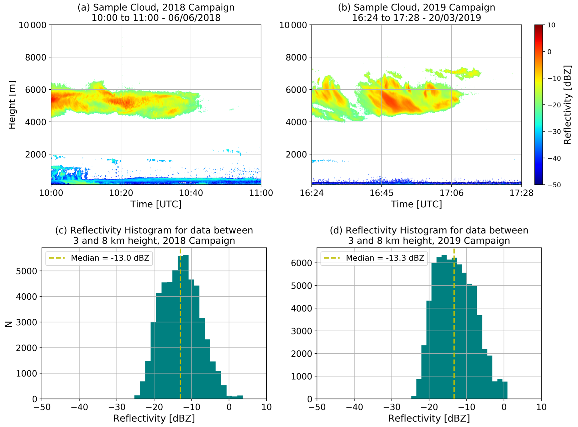
Figure 11Altostratus cloud sampled during the 2018 (a) and 2019 campaigns (b). Lower reflectivities are easier to capture at lower altitudes because of the lower distance and attenuation losses (Eq. 5b). In the altostratus reflectivity histograms (c, d) we observe that, for both campaigns, measurements are within the ranges reported in the literature.
This study presents a cloud radar calibration method that is based on a cloud radar power signal backscattered from a reference reflector. We study the validity of the method and variability in the results by performing measurements in two experimental setups and analyzing the associated results. In the first experimental setup, we use a scanning BASTA mini W-band cloud radar that is aimed towards a 20 cm triangular trihedral target installed at the top of a 20 m mast located 376.5 m from the radar. For the second experimental setup, we use the same radar, aimed towards a 10 cm triangular trihedral target mounted on a pan-tilt motor at the top of a 10 m mast. The mast is located 196 m from the radar.
The first consideration in the design of the experimental setup is the need to avoid excessive compression or saturation in the radar receiver. This must be checked before any calibration attempt by comparing the measurements of the radar backscattered power with the radar receiver power transfer curve. In both our setups, we found losses due to compression of the order of 0.2∼0.3 dB. There is a compensating effect between the target RCS and radar-to-target distance (Eq. 2b). Since the compression effect is small, we correct it using our receiver power transfer curve. However, in cases where the radar is operating close to saturation, or when compression effects are larger than the calibration uncertainty goal, it is advisable to compensate by reducing the target size or by positioning the target farther away from the radar.
Second, the reflector must be positioned far enough from the radar to be outside the antennas' near-field distance and to ensure that the received power has low antenna overlap losses. The BASTA mini cloud radar has a Fraunhofer near-field distance of 50 m. The estimated maximum overlap loss is less than 0.1 dB for the closest (10 m) mast setup. Thus, we conclude that the target positioning is far enough for both setups.
Third, the experimental setup should strive to reduce clutter in the radar measurements. This can be achieved by operating in an open field that is several hundreds of meters in length and free of trees or other signal-inducing obstacles. It is also advisable to perform radar measurements under clear conditions, without fog or rain, with the wind speed below 1 m s−1, and low turbulence.
Next, the proposed calibration method requires performing several iterations in the same setup configuration. In each iteration, the setup is first realigned, followed by approximately 1 h of sampling of the reference reflector's backscattered power. The sampled power is then corrected for compression effects, incomplete antenna overlap, variations in radar gain due to temperature and atmospheric attenuation before being used to estimate a RCS calibration term value. Once all iterations are completed, the final RCS and equivalent reflectivity calibration terms can be computed with their respective uncertainties.
Iterations are necessary because they enable the quantification of bias introduced by inevitable system misalignment. Our experiments indicate that, for our setup, at least five iterations are necessary to reach convergence in the calculation of bias and uncertainty associated with misalignment. We find a bias correction of dB for the 20 m mast and of dB for the 10 m mast. This difference can be explained by the more precise alignment attainable with the pan-tilt motor installed on the 10 m mast.
Calibration is also impacted by changes in the gain of radar components associated with internal temperature variations. For the radar used in our experiment, these changes reach up to ±0.6 dB. Our experiments enabled us to retrieve a correction function for the temperature dependence and to reduce the temperature uncertainty contribution to σT=0.23 dB. This result indicates that lower calibration uncertainties can be achieved by studying temperature effects, especially for solid-state radars.
Another necessary consideration is the inclusion of gain variations with distance which are introduced by frequency-dependent losses in the IF of the radar receiver. We found calibration variations with distance up to 0.9 dB for the 2019 campaign. Therefore, characterizing the IF loss is a necessary step for validating the calibration results for all ranges.
Our analyses reveal that the predominant source of uncertainty for all experiments is the reference target RCS, reaching approximately 2 dB due to the use of a theoretical model, instead of an experimental characterization. The next most important contributions to uncertainty come from the levels of clutter and alignment precision. These two effects have different magnitudes in our two experimental setups (10 and 20 m masts). The 20 m mast setup uncertainty is limited by the uncertainty contribution of the alignment bias estimation σΛ=0.28 dB. The 10 m mast setup uncertainty is limited by the uncertainty contribution of the signal-to-clutter ratio σSCR=0.9 dB. This result reveals that there is a tradeoff between better target alignment and additional clutter introduced by the alignment motor.
The complete uncertainty budget enables us to conclude that, to reach a calibration uncertainty under 1 dB, it is necessary to have a target RCS characterization with an uncertainty lower than 0.9 dB, based on the accumulated uncertainty of all terms, except target RCS of 0.4 dB. This uncertainty was obtained using the 20 cm target on the 20 m mast during the 2018 experiment when six target sampling iterations were performed.
Finally, because of cloud radar hardware modifications in the fall of 2018, the calibration coefficients found in May 2018 and March 2019 differ by 1.2 dB. We compare the cloud radar measurements of altostratus clouds performed in May 2018 and March 2019. The reflectivity distributions of the two events are consistent and compatible with values previously registered in the literature. The two distributions yield median values that differ by 0.3 dB.
For future work, we envisage the development of a technological solution to allow target orientation without introducing additional clutter. Another interesting prospect is to improve the accuracy of the radar scanner to enable a direct retrieval of the antenna pattern with the radar, following the method proposed by Garthwaite et al. (2015). This retrieval would improve the bias correction arising from parallax errors, which at present is calculated assuming parallel radar antennas.
We also plan to perform a receiver noise figure characterization, to further reduce uncertainty in the IF correction, and an echo chamber characterization of our reference targets. Target characterization will enable the removal of bias caused by manufacturing imprecision, reduce the RCS uncertainty contribution to total uncertainty and improve the estimation of our system misalignment bias correction.
Furthermore, there is ongoing research on calibration and antenna pattern characterization methods based on reference targets held by unmanned aerial vehicles (UAVs; Duthoit et al., 2017; Yin et al., 2019). Since the underlying principle is the same, most considerations written here should be directly applicable in these new experiments. Here the UAV takes the role of the mast, holding the reflector (usually a sphere), and therefore, it is important to characterize the UAV RCS and verify that it does not interfere with the experiment. The main difference would be in the procedure necessary for estimating bias because the reference target (usually a sphere) will always be moving due to the wind. Here an adaptation of the effective RCS simulator would be necessary to account for the target type and different alignment protocol.
| Symbol | Description | Units |
| CΓ(T,Fb) | RCS calibration term | dB(m−2 mW−1) |
| CΓ(T,F0) | RCS calibration term at the IF frequency F0 | dB(m−2 mW−1) |
| RCS calibration coefficient | dB(m−2 mW−1) | |
| Single sample of the calibration coefficient | dB(m−2 mW−1) | |
| Mean value of all samples retrieved in iteration i, | dB(m−2 mW−1) | |
| CZ(T,Fb) | Radar equivalent reflectivity calibration term | dB(mm6 m−5 mW−1) |
| δCΓ | RCS calibration uncertainty | dB |
| δCZ | Radar equivalent reflectivity calibration uncertainty | dB |
| Fb | Signal frequency at the radar receiver's IF | MHz |
| fIF(Fb) | IF loss correction function | dB |
| Γ(r) | Radar cross section of reflections at distance r | dBsm |
| Γ0 | Radar cross section of the reference target | dBsm |
| Misalignment bias correction | dB | |
| λ | Radar carrier wavelength | m |
| N | Number of iterations performed in a calibration experiment | |
| Pr(r0) | Power received from the target position r0 | dBm |
| Pr(r) | Power received from distance r | dBm |
| pt | Radar transmitted power | mW |
| r | Distance from the radar | m |
| r0 | Distance between radar and reference target | m |
| F0 | IF frequency associated with the target distance | m |
| σA | Calibration uncertainty introduced by antenna properties | dB |
| σϵ | Standard deviation between all values, used in the estimation of | dB |
| Uncertainty of the reference target RCS | dB | |
| σi | Uncertainty in the estimation of each value | dB |
| σIF | Uncertainty of the IF loss correction function | dB |
| σΛ | Uncertainty of the misalignment bias correction | dB |
| σSCR | Uncertainty introduced by clutter at the target position | dB |
| σT | Uncertainty of the temperature correction function | dB |
| θ | Antenna beamwidth | rad |
| Ze | Radar equivalent reflectivity | dBZ |
All data related to atmospheric conditions used in this study are hosted by the SIRTA observatory. Data access can be requested free of charge by following the conditions indicated in the SIRTA data policy (https://sirta.ipsl.fr/data_policy.html, last access: 3 December 2020, SIRTA, 2020b). The SIRTA observatory website can be accessed at https://sirta.ipsl.fr/ (last access: 3 December 2020, SIRTA, 2020c), and the data request form can be found at https://sirta.ipsl.fr/data_form.html (last access: 3 December 2020, SIRTA, 2020a). All radar data are distributed by the IPSL with the following identifier: https://doi.org/10.14768/6dd7bbb2-6e0d-4de3-bf03-7d6ead628845 (Toledo et al., 2020).
The supplement related to this article is available online at: https://doi.org/10.5194/amt-13-6853-2020-supplement.
All authors contributed to the planning of the campaigns and the design of the calibration experiments. JD was responsible for the radar installation and operation. JCD and FT worked on the preparation, development and operation of the necessary infrastructure for the experiments. JD and FT retrieved the power transfer curve of the radar receiver. Data analysis and the establishment of the calibration methodology presented in the paper were done by FT. MH and FT worked on defining the paper structure and content. FT, SJ and CLG worked on developing the method for retrieving the IF correction function and its calculation. CLG contributed with technical information about the radar. All authors reviewed the paper.
Felipe Toledo has received research funding from Company Meteomodem. The other authors declare that they have no conflict of interest.
The authors would like to acknowledge Johan Parra, Patricia Delville, Cristophe Boitel and Marc-Antoine Drouin from the SIRTA atmospheric observatory for their assistance with the execution of the field experiments. This acknowledgement is extended to Razvan Pirloaga and Dragos Ene from the INOE Institute, Romania. We would also like to thank Fabrice Bertrand and Jean-Paul Vinson from the LATMOS Laboratory, France, for their collaboration.
We would like to acknowledge the two reviewers for their expert comments which enabled us to improve the proposed calibration method.
Felipe Toledo acknowledges the French Association Nationale de la Recherche (ANRT) and the company Meteomodem for their contribution to the funding of this work. Finally, we state that this work is part of the ACTRIS-2 project and has received funding from the European Union's Horizon 2020 research and innovation program (grant no. 654109).
This research has been supported by the European Union's Horizon 2020 research and innovation program (ACTRIS-2 (grant no. 654109)) and the French Association Nationale de la Recherche (ANRT) and the company Meteomodem. Together, they helped fund the work of coauthor Felipe Toledo.
This paper was edited by Stefan Kneifel and reviewed by Alexander Myagkov and one anonymous referee.
Anagnostou, E. N., Morales, C. A., and Dinku, T.: The Use of TRMM Precipitation Radar Observations in Determining Ground Radar Calibration Biases, J. Atmos. Ocean. Tech., 18, 616–628, https://doi.org/10.1175/1520-0426(2001)018<0616:TUOTPR>2.0.CO;2, 2001. a
Atlas, D.: RADAR CALIBRATION, B. Am. Meteorol. Soc., 83, 1313–1316, https://doi.org/10.1175/1520-0477-83.9.1313, 2002. a
Bergada, M., Sekelsky, S. M., and Li, L.: External Calibration of Millimeter-Wave Atmospheric Radar System Using Corner Reflectors and Spheres. Eleventh ARM Science Team Meeting Proceedings, Atlanta, Georgia, 19–23 March 2001. a
Boers, R., Baltink, H. K., Hemink, H. J., Bosveld, F. C., and Moerman, M.: Ground-Based Observations and Modeling of the Visibility and Radar Reflectivity in a Radiation Fog Layer, J. Atmos. Ocean. Tech., 30, 288–300, https://doi.org/10.1175/JTECH-D-12-00081.1, 2013. a
Boucher, O., Randall, D., Artaxo, P., Bretherton, C., Feingold, G., Forster, P., Kerminen, V.-M., Kondo, Y., Liao, H., Lohmann, U., Rasch, P., Satheesh, S. K., Sherwood, S., Stevens, B., and Zhang, X. Y.: Clouds and Aerosols. In: Climate Change 2013: The Physical Science Basis. Contribution of Working Group I to the Fifth Assessment Report of the Intergovernmental Panel on Climate Change, edited by: Stocker, T. F., Qin, D., Plattner, G.-K., Tignor, M., Allen, S. K., Boschung, J., Nauels, A., Xia, Y., Bex, V., and Midgley, P. M., Cambridge University Press, Cambridge, United Kingdom and New York, NY, USA, 2013. a
Bringi, V. N. and Chandrasekar, V.: Polarimetric Doppler weather radar: principles and applications, Cambridge university press, United States of America by Cambridge University Press, New York, 2001. a
Brock, B. C. and Doerry, A. W.: Radar cross section of triangular trihedral reflector with extended bottom plate, Sandia National Laboratories Albuquerque, New Mexico 87185 and Livermore, California 94550, United States, Technical Report, Report Nos. SAND2009-2993, TRN: US201016%%1855, 7—22, https://doi.org/10.2172/984946, 2009. a, b
Brooker, G: Introduction to Sensors for Ranging and Imaging, SciTech Publishing Inc, New York, United States, 2008. a
Chandrasekar, V., Baldini, L., Bharadwaj, N., and Smith, P. L.: Calibration procedures for global precipitation-measurement ground-validation radars, URSI Radio Science Bulletin, 2015, 45–73, 2015. a, b, c, d
Delanoë, J., Protat, A., Vinson, J.-P., Brett, W., Caudoux, C., Bertrand, F., Parent du Chatelet, J., Hallali, R., Barthes, L., Haeffelin, M., and Dupont, J.-C.: Basta: a 95-GHz fmcw doppler radar for cloud and fog studies, J. Atmos. Ocean. Tech., 33, 1023–1038, 2016. a, b, c, d, e
Doviak, R. J. and Zrnić, D. S.: Doppler Radar and Weather Observations, Mineola, Dover Publications, INC, New York, 2006. a
Dupont, J.-C., Haeffelin, M., Protat, A., Bouniol, D., Boyouk, N., and Morille, Y.: Stratus–fog formation and dissipation: a 6-day case study, Bound.-Lay. Meteorol.,143, 207–225, 2012. a
Dupont, J.-C., Haeffelin, M., Wærsted, E., Delanoë, J., Renard, J.-B., Preissler, J., and O'dowd, C.: Evaluation of Fog and Low Stratus Cloud Microphysical Properties Derived from In Situ Sensor, Cloud Radar and SYRSOC Algorithm, Atmosphere, 9, 169, https://doi.org/10.3390/atmos9050169, 2018. a
Duthoit, S., Salazar, J. L., Doyle, W., Segales, A., Wolf, B., Fulton, C., and Chilson, P.: A new approach for in-situ antenna characterization, radome inspection and radar calibration, using an Unmanned Aircraft System (UAS), in: 2017 IEEE Radar Conference (RadarConf), Seattle, WA, USA, 8–12 May 2017, IEEE, 0669–0674, https://doi.org/10.1109/RADAR.2017.7944287, 2017. a
Ewald, F., Groß, S., Hagen, M., Hirsch, L., Delanoë, J., and Bauer-Pfundstein, M.: Calibration of a 35 GHz airborne cloud radar: lessons learned and intercomparisons with 94 GHz cloud radars, Atmos. Meas. Tech., 12, 1815–1839, https://doi.org/10.5194/amt-12-1815-2019, 2019. a, b, c
Fox, N. I. and Illingworth, A. J.: The retrieval of stratocumulus cloud properties by ground-based cloud radar, J. Appl. Meteorol., 36, 485–492, 1997. a, b
Garthwaite, M. C., Nancarrow, S., Hislop, A., Thankappan, M., Dawson, J. H., and Lawrie, S.: The Design of Radar Corner Reflectors for the Australian Geophysical Observing System : A single design suitable for InSAR deformation monitoring and SAR calibration at multiple microwave frequency bands, Record 2015/003, Geoscience Australia, Canberra, https://doi.org/10.11636/Record.2015.003, 2015. a, b
Gaussiat, N., Sauvageot, H., and Illingworth, A. J.: Cloud liquid water and ice content retrieval by multiwavelength radar, J. Atmos. Ocean. Tech., 20, 1264–1275, 2003. a
Haeffelin, M., Barthès, L., Bock, O., Boitel, C., Bony, S., Bouniol, D., Chepfer, H., Chiriaco, M., Cuesta, J., Delanoë, J., Drobinski, P., Dufresne, J.-L., Flamant, C., Grall, M., Hodzic, A., Hourdin, F., Lapouge, F., Lemaître, Y., Mathieu, A., Morille, Y., Naud, C., Noël, V., O'Hirok, W., Pelon, J., Pietras, C., Protat, A., Romand, B., Scialom, G., and Vautard, R.: SIRTA, a ground-based atmospheric observatory for cloud and aerosol research, Ann. Geophys., 23, 253–275, https://doi.org/10.5194/angeo-23-253-2005, 2005. a, b
Haynes, J. M., L'Ecuyer, T. S., Stephens, G. L., Miller, S. D., Mitrescu, C., Wood, N. B., and Tanelli, S.: Rainfall retrieval over the ocean with spaceborne W-band radar, J. Geophys. Res., 114, D00A22, https://doi.org/10.1029/2008JD009973, 2009. a
Hogan, R. J., Jakob, C., and Illingworth, A. J.: Comparison of ECMWF winter-season cloud fraction with radar-derived values, J. Appl. Meteorol., 40, 513–525, 2001. a
Liebe, H. J.: MPM–An atmospheric millimeter-wave propagation model, Int. J. Infrared Milli., 10, 631–650, 1989. a, b
Liebe, H. J., Manabe, T., and Hufford, G. A.: Millimeter-wave attenuation and delay rates due to fog/cloud conditions, IEEE T. Antenn. Propag., 37, 1617–1612, 1989. a
Meissner, T. and Wentz, F. J.: The complex dielectric constant of pure and sea water from microwave satellite observations, IEEE T. Geosci.Remote, 42, 1836–1849, https://doi.org/10.1109/TGRS.2004.831888, 2004. a
Mülmenstädt, J. and Feingold, G.: The radiative forcing of aerosol–cloud interactions in liquid clouds: wrestling and embracing uncertainty, Current Climate Change Reports, 4, 23–40, 2018. a
Myhre, G., Shindell, D., Bréon, F.-M., Collins, W., Fuglestvedt, J., Huang, J., Koch, D., Lamarque, J.-F., Lee, D., Mendoza, B., Nakajima, T., Robock, A., Stephens, G., Takemura, T., and Zhang, H.: Anthropogenic and Natural Radiative Forcing, in: Climate Change 2013: The Physical Science Basis, Contribution of Working Group I to the Fifth Assessment Report of the Intergovernmental Panel on Climate Change, edited by: Stocker, T. F., Qin, D., Plattner, G.-K., Tignor, M., Allen, S. K., Boschung, J., Nauels, A., Xia, Y., Bex, V., and Midgley, P. M., Cambridge University Press, Cambridge, United Kingdom and New York, NY, USA, 2013. a
Pappalardo, G.: ACTRIS Aerosol, Clouds and Trace Gases Research Infrastructure, EPJ Web Conf., 176, 09004, https://doi.org/10.1051/epjconf/201817609004, 2018. a
Pozar, D. M.: Microwave engineering, John Wiley & Sons, Inc., Hoboken, New Jersey, 2009. a
Protat, A., Bouniol, D., Delanoë, J., O’Connor, E., May, P. T., Plana-Fattori, A., Hasson, A., Görsdorf, U., and Heymsfield, A. J.: Assessment of CloudSat reflectivity measurements and ice cloud properties using ground-based and airborne cloud radar observations, J. Atmos. Ocean. Tech., 26, 1717–1741, 2009. a
Protat, A., Bouniol, D., O'Connor, E. J., Klein Baltink, H., Verlinde, J., and Widener, K.: CloudSat as a Global Radar Calibrator, J. Atmos. Ocean. Tech., 28, 445–452, https://doi.org/10.1175/2010JTECHA1443.1, 2011. a
Richardson, M.: Fundamentals of the discrete fourier transform, Sound and vibration magazine, 12, 40–46, 1978. a
Rodríguez Olivos, R.: Design, construction and testing of a 2SB receiver for the southern millimeter-wave telescope, PhD thesis, available at: http://repositorio.uchile.cl/handle/2250/133531 (last access: 3 December 2020), 2015. a
Sassen, K.: Ice cloud content from radar reflectivity, J. Clim. Appl. Meteorol., 26, 1050–1053, 1987. a
Scolnik, M. I.: Radar Handbook, 3rd edn., McCraw-Hill, New York, 2000. a
Sekelsky, S. M. and Clothiaux, E. E.: Parallax Errors and Corrections for Dual-Antenna Millimeter-Wave Cloud Radars, J. Atmos. Ocean. Tech., 19, 478–485, https://doi.org/10.1175/1520-0426(2002)019<0478:PEACFD>2.0.CO;2, 2002. a, b, c
SIRTA: Data Request Form, SIRTA/IPSL, available at: https://sirta.ipsl.fr/data_form.html, last access: 3 December 2020a. a
SIRTA: Data Policy, SIRTA/IPSL, available at: https://sirta.ipsl.fr/data_policy.html, last access: 3 December 2020b. a
SIRTA, SIRTA/IPSL, https://sirta.ipsl.fr/, last access: 3 December 2020c. a
Toledo, F., Dupont, J.-C., Delanoë, J., Haeffelin, M., Parra, J., Delville, P., Boitel, C., and Le Gac, C.: 2018 and 2019 ACTRIS Cloud Radar Calibration Campaign, Corner Reflectors on Masts Experiment, IPSL, https://doi.org/10.14768/6dd7bbb2-6e0d-4de3-bf03-7d6ead628845, 2020. a
Uttal, T. and Kropfli, R. A.: The Effect of Radar Pulse Length on Cloud Reflectivity Statistics, J. Atmos. Ocean. Tech., 18, 947–961, https://doi.org/10.1175/1520-0426(2001)018<0947:TEORPL>2.0.CO;2, 2001. a
Wærsted, E. G., Haeffelin, M., Dupont, J.-C., Delanoë, J., and Dubuisson, P.: Radiation in fog: quantification of the impact on fog liquid water based on ground-based remote sensing, Atmos. Chem. Phys., 17, 10811–10835, https://doi.org/10.5194/acp-17-10811-2017, 2017. a
Wærsted, E. G., Haeffelin, M., Steeneveld, G.-J., and Dupont, J.-C.: Understanding the dissipation of continental fog by analysing the LWP budget using idealized LES and in situ observations, Q. J. Roy. Meteor. Soc., 145, 784–804, https://doi.org/10.1002/qj.3465, 2019. a
Yau, M. K. and Rogers, R. R.: A short course in cloud physics, 3rd edn., Elsevier Science & Technology, Imprint: Butterworth-Heinemann Ltd, Oxford, United Kingdom, 1996. a
Yin, J., Hoogeboom, P., Unal, C., Russchenberg, H., Van der Zwan, F., and Oudejans, E.: UAV-Aided Weather Radar Calibration, IEEE T. Geosci. Remote, 57, 10362–10375, https://doi.org/10.1109/TGRS.2019.2933912, 2019. a
- Abstract
- Introduction
- Equations used in radar calibration
- Experimental setup
- Methodology
- Sources of uncertainty and bias in absolute calibration with corner reflectors
- Results
- Conclusions
- Appendix A: Table of symbols
- Data availability
- Author contributions
- Competing interests
- Acknowledgements
- Financial support
- Review statement
- References
- Supplement