the Creative Commons Attribution 4.0 License.
the Creative Commons Attribution 4.0 License.
 | 21 Dec 2020
Applying deep learning to NASA MODIS data to create a community record of marine low-cloud mesoscale morphology
Robert Wood
Johannes Mohrmann
Kerry Meyer
Lazaros Oreopoulos
Steven Platnick
Marine low clouds display rich mesoscale morphological types and distinct spatial patterns of cloud fields. Being able to differentiate low-cloud morphology offers a tool for the research community to go one step beyond bulk cloud statistics such as cloud fraction and advance the understanding of low clouds. Here we report the progress of our project that aims to create an observational record of low-cloud mesoscale morphology at a near-global (60∘ S–60∘ N) scale. First, a training set is created by our team members manually labeling thousands of mesoscale (128×128) MODIS scenes into six different categories: stratus, closed cellular convection, disorganized convection, open cellular convection, clustered cumulus convection, and suppressed cumulus convection. Then we train a deep convolutional neural network model using this training set to classify individual MODIS scenes at 128×128 resolution and test it on a test set. The trained model achieves a cross-type average precision of about 93 %. We apply the trained model to 16 years of data over the southeastern Pacific. The resulting climatological distribution of low-cloud morphology types shows both expected and unexpected features and suggests promising potential for low-cloud studies as a data product.
- Article
(5052 KB) - Full-text XML
- BibTeX
- EndNote


Marine low clouds are important for the mass, heat, and momentum transport in the planetary boundary layer (PBL) and between the PBL and free troposphere, the radiative energy balance of the climate, and the magnitude of feedback strength under climate change. Observations of marine low clouds are indispensable for advancing our understanding of these clouds for deriving new theories and insights and for model validation and constraining. Modern satellite observations have the advantage of providing global and long-term coverage. Current satellite products offer detailed pixel-level retrievals of cloud properties such as cloud optical depth, cloud droplet effective radius, and cloud phase. Most cloud classification schemes are based on either single pixel measurements or joint histograms of two cloud properties.
However, marine low clouds are known to have various mesoscale morphology types since first satellite observations of clouds became available (Agee and Dowell, 1974). These mesoscale morphology types are created by the characteristic patterns into which clouds are organized (Fig. 1). Cloud mesoscale morphology types are not only phenological classifications of satellite images, but also a manifestation of a complex mixture of underlying physical processes (Atkinson and Zhang, 1996; Stevens et al., 2005; Wang and Feingold, 2009; Wood, 2012; Wood and Hartmann, 2006). These physical processes are critical for fundamental understanding and better modeling of marine low clouds because of their impact on mass, heat, and momentum transport, on radiative energy balance, and their feedbacks to climate change. Wood and Hartmann (2006) trained a two-layer neural network on probability distribution functions and 2-D power spectra of liquid water path to classify cloud morphology into four categories for 256×256 scenes. The method has been successfully used to analyze morphology types and associated cloud properties (McCoy et al., 2017; Muhlbauer et al., 2014).
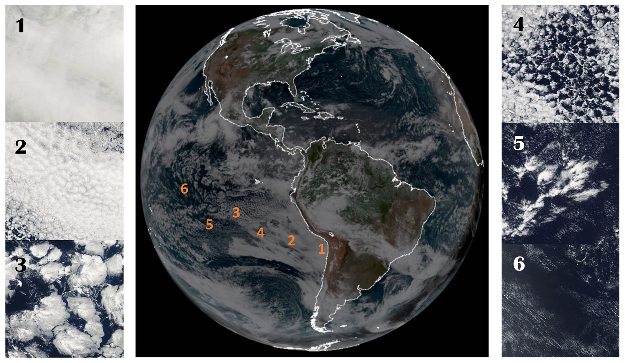
Figure 1A full disk image of GOES-16 on 6 August 2018 and six scenes of MODIS images at smaller scales representing different morphology types at corresponding locations in the GOES image. Except scene 1, all scenes are from the same day. Scene 1 is from a different day because there were no representative stratus scenes on this day in the southeastern Pacific region.
Here we introduce a NASA-funded project to classify marine low-cloud observations into six different mesoscale morphology types based directly on full images without engineering features. The goal is to produce a community data record that spans about two decades at near-global scales that will enable the research community to go beyond bulk cloud statistics and will advance our understanding of low-level mesoscale convective clouds through exploiting the rich spatial information content of observations. Section 2 describes the data and methodology; Sect. 3 introduces preliminary results, and Sect. 4 gives discussions of future plans and outlook of the data product; Sect. 5 concludes.
2.1 Data source
The primary observational data for this study are from the MODerate resolution Imaging Spectrometer (MODIS) on board the Aqua satellite. We use reflectance from channels 1 (0.65 µm), 3 (0.47 µm), and 4 (0.55 µm) and cloud optical depth, cloud droplet effective radius, cloud mask, and cloud top height from the MODIS cloud product (Platnick et al., 2017) in building up the training set. The spatial resolution of these parameters is 1 km at nadir. The cloud optical depth and effective radius retrievals are combined to produce the cloud liquid water path (Platnick et al., 2017). Reflectance from channel 4 is used for deep neural network model training and inference, while the other MODIS observations and products are used for data quality control, filtering, and contextual information, as explained below.
We first break MODIS images into 128×128 pixel scenes. The selection of 128×128 results from a balance because larger sizes suffer from too much mixing of different types in a scene, while smaller sizes contain not enough contextual information for classification. We filter out scenes that contain a significant fraction of high clouds (no more than 10 %), defined as pixels with cloud top height above 6 km, or whose low-cloud fraction is lower than 5 %. We also exclude scenes whose viewing zenith angle is greater than 45∘. Scenes with more than 10 % land coverage are also excluded. The resulting scenes are treated as dominated by marine low clouds.
For training purposes, we create auxiliary images that contain the broad context of the scene of interest and distributions of the liquid water path and cloud top height for the scene (Fig. 2). The scene image, together with the auxiliary images, is presented to a panel of human experts on the Zooniverse platform (https://www.zooniverse.org/projects/cloud-class/clouds-with-a-type, last access: 28 November 2020) for manual labeling. We intend to use the same platform in the future to crowdsource the labeling task.
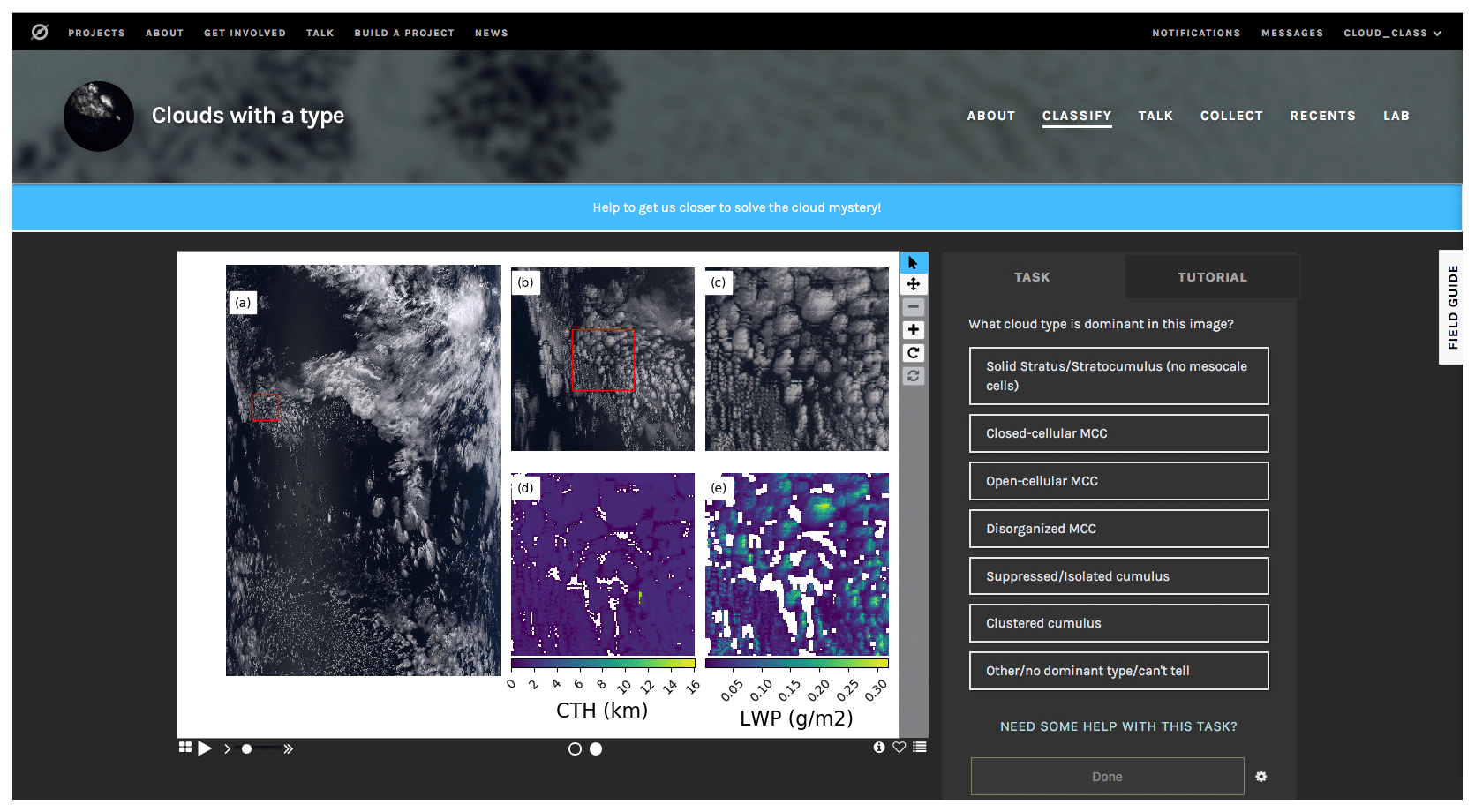
Figure 2The Zooniverse interface for manual labeling. The center image is made up of five panels. Panel (a) shows the full granule (usually 2030×1350 pixels) true-color image for a large context. Panel (b) shows a portion of the granule immediately surrounding the scene to be labeled, outlined by the red square. Panel (c) shows the visible scene image while panels (d, e) show the cloud top height and liquid water path fields in the scene to be labeled. The panels to the right of the center image show labeling choices. The tutorial document is available by clicking on the “FIELD GUIDE” tab on the right side. Additional options for scenes with heavily mixed types, scenes with sea ice, or scenes with other issues are found in the “other” menu. The image is a screenshot of our Zooniverse project.
Spatiotemporally collocated Modern-Era Retrospective analysis for Research and Applications, version 2 (MERRA-2) (Gelaro et al., 2017) data are used to provide meteorological variables for each scene.
Morphology types
Marine low-cloud mesoscale morphology patterns are extremely diverse. In order to keep the task manageable, we settle on six representative types. These are stratus, closed cellular convection, disorganized cellular convection, open cellular convection, clustered cumulus, and suppressed cumulus (Fig. 3). These types are by no means exhaustive given the diversity of observable patterns. However, these six types are the most common and largely representative of the data when we inspect a large collection of scenes. In the current version, each low-cloud scene will be assigned one of these six types. We also believe that these types have distinct underlying physical processes. Stratus is mostly created by relatively uniform radiative cooling or driven by synoptic weather systems such as fronts, while closed cellular convection is driven by radiative cooling and organized into distinctive honeycomb mesoscale patterns. Disorganized cellular convection is characterized by a combination of elements of convection and a large portion of stratiform clouds that tend to have large droplet sizes and small cloud optical depths, creating their characteristic appearance. Their cellular sizes are typically larger, on the order of 100 km, compared to closed cellular convection, on the order of 10 km. Open cellular convection is characterized by cells that are clear in the center and exhibit vigorous shallow convection around it. These convective clouds are often precipitating based on satellite and ship-based observations, which is a likely driving force that creates and maintains this mesoscale morphology type (Wang and Feingold, 2009). Clustered cumulus convection is made up of shallow, vigorous convective elements that aggregate together, accompanied by scattered shallower and optically thinner cumulus clouds nearby. The suppressed cumulus type is dominated by individual, scattered cumulus clouds that can sometimes have patterns like lines and branches.
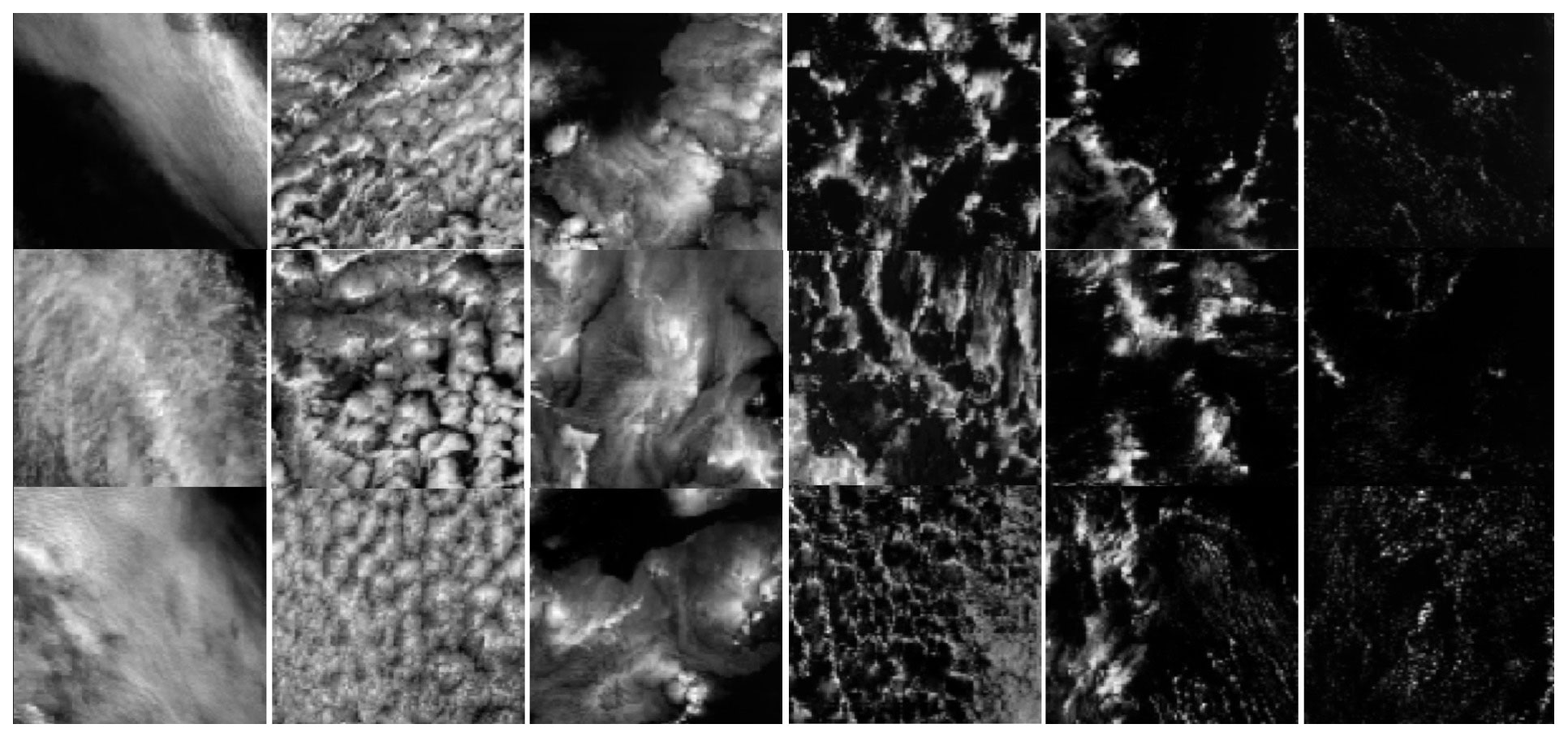
Figure 3Example scenes of MODIS single-channel images for the six different types. From left to right: stratus, closed cellular, disorganized cellular, open cellular, clustered cumulus, and suppressed cumulus types. Images taken by the NASA MODIS.
2.2 Method
To illustrate the difficulty of classifying morphology types using one-point statistics such as histograms, we show the mean probability density functions (PDFs) of cloud optical depth and droplet effective radius for each type in Fig. 4. We randomly select 1000 scenes for each cloud type from 2006 data in the southeastern Pacific region. The significant overlap between PDFs of different types makes it quite hard to classify the scenes based on these PDFs. On the other hand, deep convolutional neural network (DCNN) models have been shown to separate complex patterns into different categories at a human level (LeCun et al., 2015). We apply a transfer learning approach to our classification task in a supervised fashion, although separate efforts of unsupervised training also seem promising (Yuan, 2019).
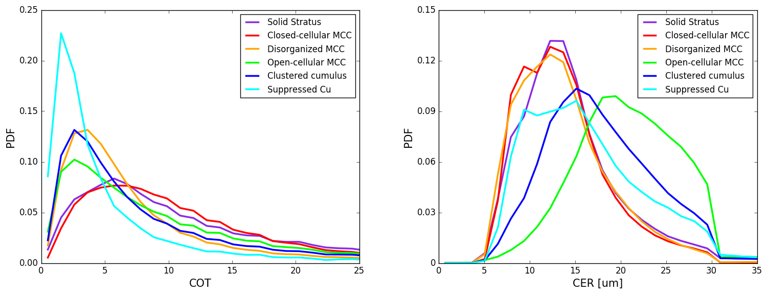
Figure 4PDFs of cloud optical depth and cloud effective radius for six morphology types. We randomly selected 1000 samples for each type, and mean distributions are shown here. Significant overlaps are observed for PDFs of both variables among different morphology types.
Specifically, we use a pretrained model (Simonyan and Zisserman, 2015) as a feature extractor and fine-tune it with our training set. The pretrained model is a 16-layer DCNN that is trained on the large-scale ImageNet dataset (Deng et al., 2009). Its weights are fixed. We add three additional layers to the pretrained model, called VGG-16, and train the resulting full model on our training set, the fine-turning step. The output of the full DCNN model is a six-element vector whose elements sum up to 1 and are interpreted as the probability that the model assigns to one of the corresponding types. We assign every scene to the type that has the highest probability, and therefore effectively we have a metric to measure how confident the model is for each classification, which provides useful information for users who may apply filters to the data.
To build the training set, our team together with several expert-level volunteers first manually labeled thousands of scenes using the Zooniverse online tool. We retain only those scenes that are unambiguously belonging to a certain type to present the best possible training set, which includes hundreds of samples for each type. We augment the training set by rotating each scene by 90 and 180∘ and also flipping the open cellular scenes to increase their sample size. The flipping operation is achieved by mirroring the original image across a horizontal axis.
Here we report results for the training, show the classification at work at a granule level and for two typical low marine low-cloud regimes: winter time midlatitude region downwind of the east coast of USA and Canada and the subtropical southeastern Pacific region.
3.1 Training performance
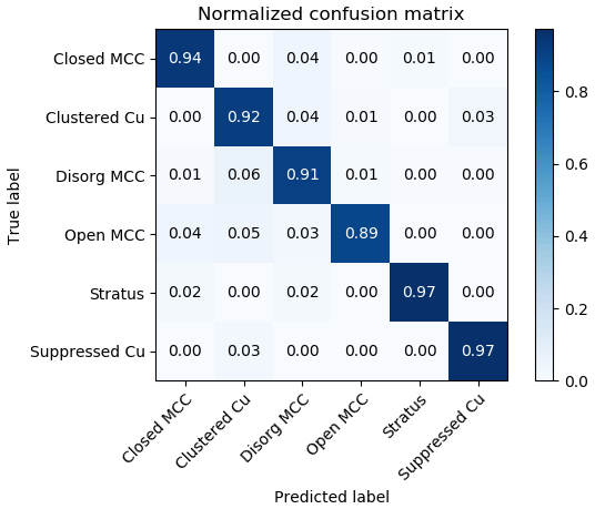
The training asymptotically converges to a plateau in terms of accuracy pretty quickly, within about 30 epochs (Fig. 5). Around epoch 30, the validation accuracy reaches a maximum. The training and validation accuracies are at around 98 % and 93 %. We save the model configuration with the best validation accuracy. After training, the model is applied to a test set that it has never seen before. The resulting confusion matrix is shown in Fig. 6. The confusion matrix summarizes the classification prediction results. For each cloud type, or row, it shows the percentage of correct predictions on the diagonal and percentages of incorrect predictions off the diagonal. The trained model achieves an average precision of about 93 % across different types. Open cellular and disorganized cellular convection are the two morphology types with the lowest accuracy mainly because they had the lowest number of training samples. With a further increase in training samples in the future, we are confident that corresponding accuracies can be further improved. The biggest challenge for the model comes from separating disorganized cellular, open cellular, and clustered cumulus types. It is also worth noting that there is inherent uncertainty with the classification since even expert labelers sometimes disagree on the same scenes.
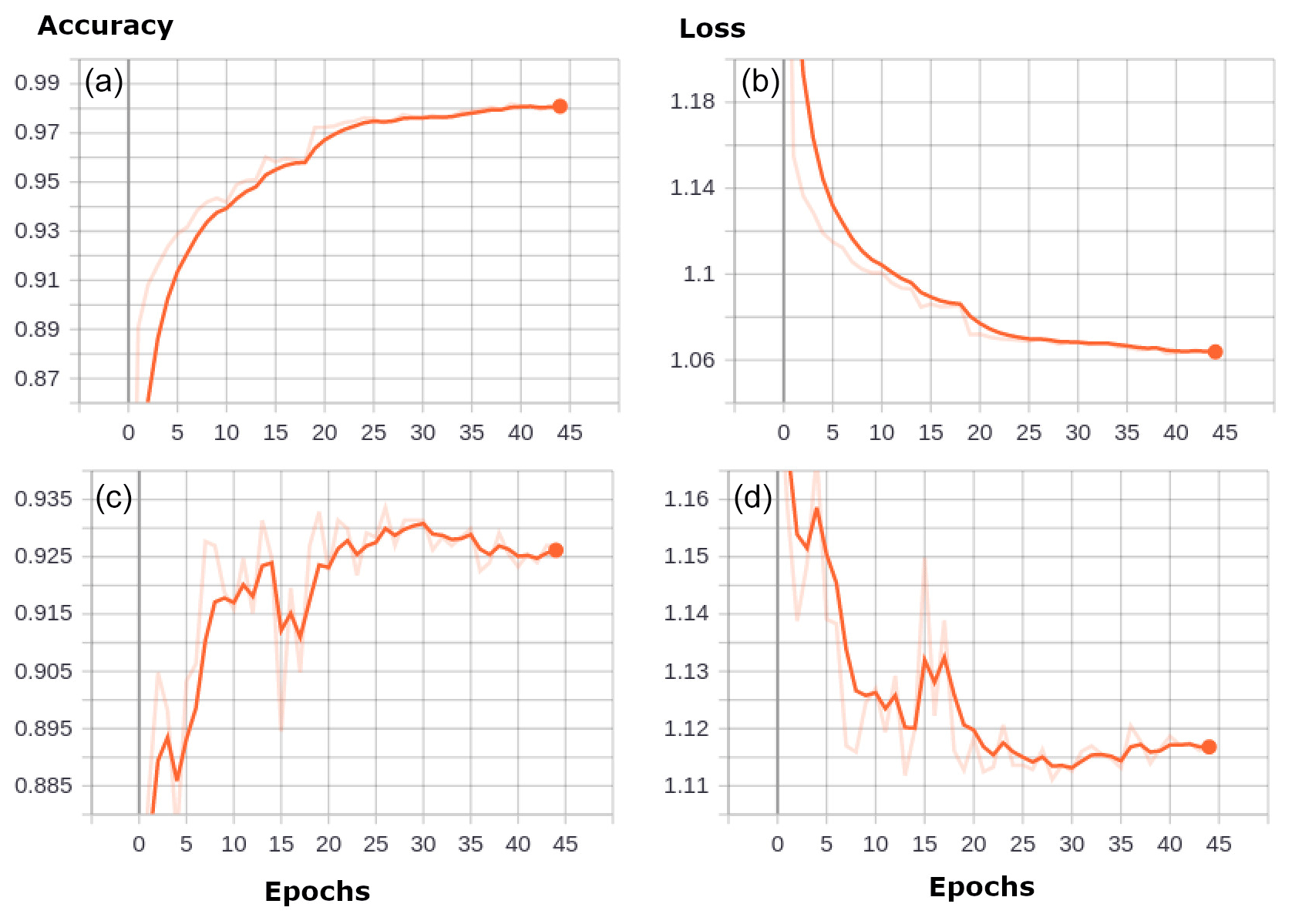
Figure 5Training (a, b) and validation (c, d) accuracy and loss trajectories. By around epoch 30, the validation accuracy peaks while validation loss bottoms out, and the training loss and accuracy asymptotically reach their minimum and maximum, respectively, which indicates further training may be overfitting the model.
3.2 An example granule
An example of a classified MODIS granule is shown in Fig. 7. The classification results are overlaid on the visible MODIS image as colored circles whose position represents the center of corresponding 128×128 scene. This is a low-cloud-dominated granule with a complex mix of different morphology types. The few missing scenes within the viewing zenith angle limits are due to subvisible high clouds overlapping the visible low clouds, which is not rare even for these low-cloud-dominated regions (Yuan and Oreopoulos, 2013), as well as a couple of scenes with too few low clouds. One can visually confirm that the model performs quite well in picking up morphology types and their transitions, corroborating the results in Fig. 5. It is worth noting that a scene does not have to be fully occupied by a cloud type to be classified into this particular type. For example, the scene centered around 14∘ S and 78∘ W is partially occupied by stratus and nonetheless classified as stratus.
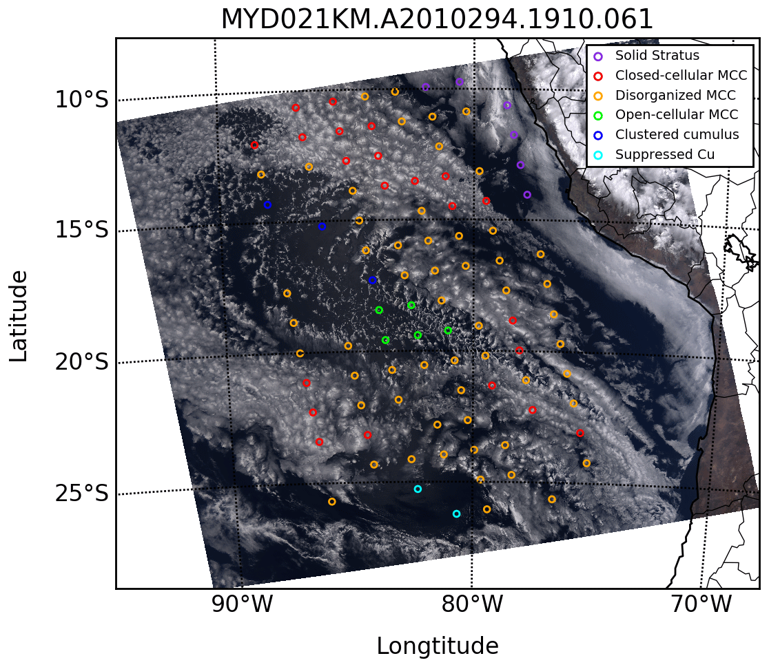
Figure 7An example granule illustrating the results of the classification algorithm. This is quite a complex granule with different morphology types mixed together. The left and right margins are not classified because the current algorithm filters out scenes whose sensor viewing zenith angles are greater than 45∘. The image is taken by NASA MODIS.
3.3 Test run over the wintertime northwestern Atlantic
During the winter, there can be many cold-air outbreak events over the northwestern Atlantic region. They create maritime low-cloud systems with various mesoscale morphology types. We apply our model to data in the winter of 2011. We first filter the raw data to include only marine low-cloud scenes using the criteria discussed in Sect. 2. The 128×128 pixel scenes are fed into the trained DCNN model for classification. For each scene, we record its morphology type, geolocation, and time and save the 2-D MODIS cloud retrieval parameters such as cloud optical depth, cloud droplet effective radius, and cloud top pressure. In this run, we do not oversample the data and therefore scenes do not overlap with each other.
Figure 8 shows frequency of occurrence maps for each cloud type along with surface wind vectors. Stratus clouds dominate in the Hudson Bay and Labrador Sea. They also frequently appear over waters around Newfoundland and, to a lesser degree, along the east coast of USA and Canada. There is also a local maximum in the western part of the Gulf of Mexico. Closed cellular type dominates the warm water of the Gulf Stream where cold continental air meets the warm water, which induces a large flux of moisture and heat from the ocean into the boundary layer and gives rise to formation of low clouds. These low clouds mostly appear as the closed cellular type according to MODIS. The disorganized type only appears in a significant quantity in the subtropics away from the coast. Open cellular clouds peak in the area south of the Greenland Sea and in the Labrador Sea and have a local maximum that is centered around 60∘ W and 35∘ N. Both are downwind of the closed cellular cloud peaks. The clustered and suppressed cumulus clouds mostly occur in the subtropics and tropics.
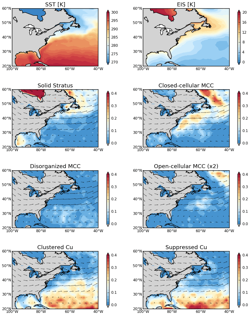
Figure 8Frequency distributions of six morphology types obtained from the classification algorithm in the northwestern Atlantic region off the east coasts of USA and Canada in the winter of 2011. The top two panels show the SST and EIS distributions using MERRA-2. Seasonal mean wind vectors at 850 hPa are plotted to illustrate the flow. We double the values for frequency of the open-cellular type to make them numerically comparable with other types.
3.4 Results over the southeastern Pacific region
We obtained all relevant Aqua MODIS level-1b and level-2 files for the southeastern Pacific region (5–45∘ S, 70–125∘ W) between 2003 and 2018. The total volume of data is about 30 TB. This region is well known for semi-permanent stratocumulus clouds.
Figure 9 shows the 16-year climatology of sea surface temperature (SST), estimated inversion strength (EIS) (Wood and Bretherton, 2006), and frequency of occurrence maps for each morphology type in the southeastern Pacific region. The frequency is normalized by the number of total MODIS scenes, including both low-cloud and non-low-cloud ones.
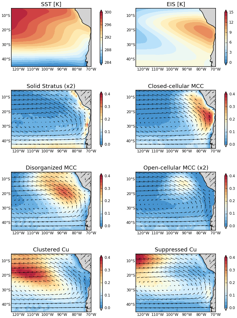
Figure 9Frequency distributions of various morphology types obtained from the classification algorithm in the subtropical eastern Pacific off the coast of South America for the period 2003–2018. The top two panels show the SST and EIS climatology from MERRA-2 for the same period. Note the doubling of scale on the stratus and open-cellular types.
Stratus clouds predominantly occur near coastal upwelling regions in the subtropics as well as in the midlatitude regions south of 40∘. Both features agree with our expectations. Stratus can still occur in other parts of the domain, but with frequencies generally below 10 %. Their frequency significantly drops away from the local maxima in the midlatitudes and along the coast. The local maxima of stratus occurrence frequency coincide spatially with cold SST.
The closed cellular type occurs most frequently about 500 km away from the coastlines. The absolute maximum is located around 27∘ S and 75∘ W, which is also where EIS peaks. Indeed, the frequency of closed cellular type roughly correlates with the EIS pattern. The frequency of this type drops off from its peak location more gradually compared to that of the stratus. Its frequency is nevertheless below 10 % west of 90∘ W, and the direction of the frequency of occurrence gradient is almost east to west. The location of peak frequency for the disorganized type is further away from the coast and occurs around 21∘ S and 89∘ W. The frequency map of this type also has an overall correlation with the EIS west of 90∘ W.
The frequency map for the open cellular type is the most distinct. Its peak features a bull's-eye pattern and occurs further downwind of the peak of the disorganized type, with a peak frequency of only about 10 %. This type also appears relatively frequently in the midlatitudes associated with midlatitude cyclones. Its spatial pattern has no direct correlation with either EIS or SST patterns, possibly implying internal mechanisms that are responsible for their appearances. Both the closed and open cellular locations agree qualitatively with the findings of Wood and Hartmann (2006), although the addition of other cloud types resulted in lower frequencies of these types in our dataset. It is also worth mentioning that the disorganized cellular type has a different geographic occurrence when compared to the findings of Wood and Hartmann (2006). This is because under that classification scheme, “disorganized” includes the bulk of scenes which we classify as suppressed and clustered; the more narrowly defined disorganized cellular type in our classification is geographically more closely associated with the other cellular cloud types. The clustered cumulus type occurrence appears to have a general anticorrelation with the EIS map. The suppressed cumulus type occurs most frequently in the tropics where the SST is the warmest.
4.1 Notable new insights
Open cellular clouds are less prevalent than previously thought (Atkinson and Zhang, 1996; McCoy et al., 2017; Muhlbauer et al., 2014), especially in subtropical regions. We attribute this to the combination of advanced quantitative observation techniques developed here and the delineation of clustered cumulus and open cellular types. The early studies did not have comprehensive observations to rely on. The more recent results may have included the two types together into the open cellular type, which overestimated the occurrence frequency of the open cellular type in the subtropics. However, given the relatively minor presence of clustered cumulus type in the midlatitudes, the open cellular type may indeed be quite prevalent there, which agrees with previous studies.
There is a strong spatial correlation between both EIS and SST and the frequency of stratus in the two regions analyzed, especially north of 35∘ N, suggesting a strong control of atmospheric stability and cold SST on this cloud type in higher-latitude regions. Their control on other cloud types may not be as tight given the loose spatial correspondence between both EIS and SST and the frequency of other cloud types, implying either other large-scale variables are in control or internal cloud processes are more important. We will leave such explorations for future studies.
4.2 Expanding the scale of test runs and further analysis
We plan to expand the test run to near-global scales for about two years. These runs will include time periods that overlap those of several field campaigns that have rich in situ and ground and airborne remote sensing data. Together with these datasets, the satellite product will help to advance the understanding of low-cloud mesoscale morphology. The global scale will also allow us to examine the general distributions of morphology types and intercompare the characteristics of low-cloud morphology in different ocean basins. Further data analysis of the current test run and future runs will target questions related to the variability of low-cloud morphology and its driving forces. We plan to release part or all of the test run results to beta testers for feedback and test use from the community.
4.3 Collocating with other satellite sensors and meteorology
We plan to collocate each classified low-cloud scene with data from sensors like CloudSat cloud profiling radar, CALIOP lidar, the Advanced Microwave Scanning Radiometer for EOS (AMSR-E and AMSR-2), and Atmospheric InfraRed Sounder (AIRS) as well as the MERRA-2 reanalysis products. Such a collocated set of variables will be useful to the research community for studying the behavior of low-cloud morphology under different environmental conditions.
4.4 Further improvement of the model
The current model works pretty well overall, particularly for closed cellular, suppressed cumulus, and clustered cumulus types. However, there is room for improvement for other types. We target two fronts for improvement: improving the model itself and increasing the quality and quantity of training data. For the former goal, we plan to test different pretrained models and what features to keep and how to best set up the classifier on top of these extracted feature vectors. For the latter goal, we have developed analysis tools to help us understand the agreement among human experts in the training set. This helps us to target types that need the improvement. We will use the Zooniverse tool to achieve this. Further increase in training data also allows us to better characterize the uncertainty in expert labeling of each category. We are looking for expert-level volunteers to join us in increasing the training sample size.
4.5 Increasing the number of types
Some of the mesoscale types can be further divided into subtypes. For example, the frequency of suppressed cumulus type is quite high in the low latitudes, and based on the manual labeling they could be further divided into multiple subtypes. We will explore the feasibility of this by assessing resource constraints and the feedback from the community.
We have developed a working deep neural network model to automatically classify cloudy scenes into six mesoscale morphology types. Initial test run results showed promising results for the southeastern Pacific and northwestern Atlantic. Using the tool, we plan to extend the dataset and create a community mesoscale morphology type product for low marine clouds observed by MODIS. We will further develop the product and actively look forward to community involvement such as beta testing, volunteering, and user feedback.
All MODIS data can be accessed using the public website: https://ladsweb.modaps.eosdis.nasa.gov/ (last access: 28 November 2020, LAADS DAAC, 2020).
TY implemented the method to train the network model. HS, JM, and TY prepared the training data. All coauthors contributed to compiling the training dataset. TY wrote the manuscript with contributions from all coauthors.
The authors declare that they have no conflict of interest.
Authors except SP are funded by NASA's Making Earth Science Data Records for Use in Research Environments (MEaSUREs) Program. The program is managed by Lucia Tsaoussi.
This research has been supported by the NASA's MEaSUREs Program (grant no. 80NSSC18M0084).
This paper was edited by Sebastian Schmidt and reviewed by two anonymous referees.
Agee, E. M. and Dowell, K. E.: Observational Studies of Mesoscale Cellular Convection, J. Appl. Meteor., 13, 46–53, https://doi.org/10.1175/1520-0450(1974)013<0046:OSOMCC>2.0.CO;2, 1974.
Atkinson, B. W. and Zhang, W. J.: Mesoscale shallow convection in the atmosphere, Rev. Geophys., 34, 403–431, https://doi.org/10.1029/96RG02623, 1996.
Deng, J., Dong, W., Socher, R., Li, L.-J., Li, K., and Li, F. F.: ImageNet: A large-scale hierarchical image database, IEEE Computer Vision and Pattern Recognition (CVPR), 248–255, 2009.
Gelaro, R., McCarty, W., Suarez, M. J., Todling, R., Molod, A., Takacs, L., Randles, C. A., Darmenov, A., Bosilovich, M. G., Reichle, R., Wargan, K., Coy, L., Cullather, R., Draper, C., Akella, S., Buchard, V., Conaty, A., da Silva, A. M., Gu, W., Kim, G.-K., Koster, R., Lucchesi, R., Merkova, D., Nielsen, J. E., Partyka, G., Pawson, S., Putman, W., Rienecker, M., Schubert, S. D., Sienkiewicz, M., and Zhao, B.: The Modern-Era Retrospective Analysis for Research and Applications, Version 2 (MERRA-2), J. Climate, 30, 5419–5454, https://doi.org/10.1175/JCLI-D-16-0758.1, 2017.
LAADS DAAC, NASA, Goddard Space Flight Center, https://ladsweb.modaps.eosdis.nasa.gov/, last access: 28 November 2020.
LeCun, Y., Bengio, Y., and Hinton, G.: Deep learning, Nature, 521, 436–444, https://doi.org/10.1038/nature14539, 2015.
McCoy, I. L., Wood, R., and Fletcher, J. K.: Identifying Meteorological Controls on Open and Closed Mesoscale Cellular Convection Associated with Marine Cold Air Outbreaks, J. Geophys. Res., 122, 678–702, https://doi.org/10.1002/2017JD027031, 2017.
Muhlbauer, A., McCoy, I. L., and Wood, R.: Climatology of stratocumulus cloud morphologies: microphysical properties and radiative effects, Atmos. Chem. Phys., 14, 6695–6716, https://doi.org/10.5194/acp-14-6695-2014, 2014.
Platnick, S., Meyer, K. G., King, M. D., Wind, G., Amarasinghe, N., Marchant, B., Arnold, G. T., Zhang, Z., Hubanks, P. A., Holz, R. E., Yang, P., Ridgway, W. L., and Riedi, J.: The MODIS Cloud Optical and Microphysical Products: Collection 6 Updates and Examples From Terra and Aqua, IEEE T. Geosci. Remote., 55, 502–525, https://doi.org/10.1109/TGRS.2016.2610522, 2017.
Simonyan, K. and Zisserman, A.: Very Deep Convolutional Networks for Large-Scale Image Recognition, arXiv [preprint], arXiv:1409.1556, 2015.
Stevens, B., Vali, G., Comstock, K., Wood, R., van Zanten, M. C., Austin, P. H., Bretherton, C. S., and Lenschow, D. H.: Pockets of open cells and drizzle in marine stratocumulus, B. Am. Meteorol. Soc., 86, 51–58, https://doi.org/10.1175/BAMS-86-1-51, 2005.
Wang, H. and Feingold, G.: Modeling mesoscale cellular structures and drizzle in marine stratocumulus. Part I: Impact of drizzle on the formation and evolution of open cells, J. Atmos. Sci., 66, 3237–3256, https://doi.org/10.1175/2009JAS3022.1, 2009.
Wood, R.: Stratocumulus Clouds, Mon. Weather Rev., 140, 2373–2423, https://doi.org/10.1175/MWR-D-11-00121.1, 2012.
Wood, R. and Bretherton, C. S.: On the relationship between stratiform low cloud cover and lower-tropospheric stability, J. Climate, 19, 6425–6432, https://doi.org/10.1175/JCLI3988.1, 2006.
Wood, R. and Hartmann, D. L.: Spatial variability of liquid water path in marine low cloud: The importance of mesoscale cellular convection, J. Climate, 19, 1748–1764, 2006.
Yuan, T.: Understanding Low Cloud Mesoscale Morphology with an Information Maximizing Generative Adversarial Network, EarthArXiv, https://doi.org/10.31223/osf.io/gvebt, 2019.
Yuan, T. and Oreopoulos, L.: On the global character of overlap between low and high clouds, Geophys. Res. Lett., 40, 5320–5326, https://doi.org/10.1002/grl.50871, 2013.