Cirrus cloud shape detection by tomographic extinction retrievals from infrared limb emission sounder measurements

An improved cloud-index-based method for the detection of clouds in limb sounder data is presented that exploits the spatial overlap of measurements to more precisely detect the location of (optically thin) clouds. A second method based on a tomographic extinction retrieval is also presented. Using CALIPSO data and a generic advanced infrared limb imaging instrument as examples for a synthetic study, the new cloud index method has a better horizontal resolution in comparison to the traditional cloud index and has a reduction of false positive cloud detection events by about 30 %. The results for the extinction retrieval even show an improvement of 60 %. In a second step, the extinction retrieval is applied to real 3-D measurements of the airborne Gimballed Limb Observer for Radiance Imaging in the Atmosphere (GLORIA) taken during the Wave-driven ISentropic Exchange (WISE) campaign to retrieve small-scale cirrus clouds with high spatial accuracy.

1 Introduction

Clouds, and in particular cirrus clouds, play an important part in the radiative balance of the atmosphere. The effect of cirrus clouds in a changing climate is still uncertain, even though a change in frequency of occurrence is well established due to a redistribution of water vapor in the troposphere (IPCC, 2007; Heymsfield et al., 2017).

To increase our understanding of cirrus clouds, rigorous observations are required on their frequency, occurrence, coverage, particle sizes, number concentration, ice water content, and altitude. To generate a sufficient statistical basis for modeling and validation, global measurements of cirrus clouds are required, which can only be generated by satellite-borne instruments (e.g., Krämer et al., 2020). Owing to the dryness of the upper troposphere, cirrus clouds often generate only weak signatures in observations by remote sensing instruments, especially nadir-viewing ones. Our knowledge about clouds has been advanced greatly in recent times by the active lidar Cloud-Aerosol Lidar with Orthogonal Polarization (CALIOP) on Cloud-Aerosol Lidar and Infrared Pathfinder Satellite Observation (CALIPSO; Winker et al., 2009). Due to its active nature, it is the most highly resolving and precise satellite instrument with a cirrus cloud product that has been used successfully to create first climatologies (Nazaryan et al., 2008). Other, passive, nadir-viewing instruments often have difficulty detecting ultra-thin cirrus or properly determining the top altitude of the clouds with the necessary accuracy to determine, e.g., the radiative effects. While some advances have been made recently, e.g., by Kox et al. (2014), using data from the SEVIRI instrument on MSG (Meteosat Second Generation; Schmetz et al., 2002), these data products currently lack proper error estimates due to the nature of the classification algorithms used. The most sensitive passive methods to detect cirrus from space are in any case provided by limb-observing instruments. As cirrus clouds are typically horizontally more elongated than vertically, a limb-viewing instrument has a longer path within the cloud, generating a stronger signal and also a much higher vertical resolution. This is true for both occultation and passive emission measuring instruments. While occultation instruments are even more sensitive, passive instruments have the advantage of a much higher measurement density necessary to generate a profound global statistical basis. A historical disadvantage of limb sounders is a poor horizontal resolution compared to nadir-viewing ones, but recent developments of tomographic evaluation schemes in combination with proposed instruments with a higher measurement density level the playing field (Griessbach et al., 2020b).

While tomographic retrievals have become state of the art for limb sounders in general (e.g., Livesey and Read, 2000; Carlotti et al., 2001; Steck et al., 2005; Livesey et al., 2006; Christensen et al., 2015), in-orbit instruments do not oversample extensively; e.g., the Michelson Interferometer for Passive Atmospheric Sounding (MIPAS) instrument on ENVISAT (Fischer et al., 2008) was operated to have nonoverlapping lines of sight in the tangent layer in nominal measurement modes. Tomography was, due to instrument limitations, mostly performed to increase the retrieval accuracy in the presence of gradients in retrieved quantities along the line of sight. Hence, this study evaluates the potential capabilities of near-future limb sounders, employing imaging detectors with a much higher measurement density, simply called IRLS (Imaging IR Limb Sounder) in this study. The hypothetical instrument is largely based on the PREMIER IRLS instrument (Process Exploration through Measurement of infrared and millimeter-wave Emitted Radiation; Ungermann et al., 2010; ESA, 2012), proposed for ESA's Earth Explorer program.

The cloud index is a well proven method for the detection of clouds in infrared spectra (Spang et al., 2001a, 2008, 2012). We show how the spatial resolution and accuracy of the cloud index method can be improved upon by the so-called oversampling, where limb sounders measure spectra so frequently that the lines of sight of succeeding measurements overlap within the tangent layer. In addition to an enhancement of the cloud index method, we also investigate the capabilities of a tomographic extinction retrieval that employs the same techniques also used for the tomographic retrieval of temperature and trace gases. Previous studies have shown that tomographic methods can increase the horizontal resolution of data products gained from limb sounders, ideally up to the spacing between consecutive measurements (von Clarmann et al., 2009; Ungermann et al., 2011; Krisch et al., 2018). Here, we want to investigate how that result typically valid for optically thin conditions transfers itself to optically thicker clouds. To complement the work with synthetic measurements, the final part of this paper applies the extinction tomography to evaluate a tomographic measurement of cirrus clouds made by the Gimballed Limb Observer for Radiance Imaging in the Atmosphere (GLORIA) (Riese et al., 2014; Friedl-Vallon et al., 2014). This airborne instrument points at a 90^∘ angle in relation to the heading of its carrier and thus has a very different measurement geometry compared to along-track-pointing satellite instruments. In this sense it is a very hard test case for the method as this geometry makes the retrieval much more involved and complicated.

This paper is structured as follows. We will first briefly present the employed data products and the models and instruments they were derived from. Section 3 presents the new algorithms and methods that are then studied in depth in Sect. 4. We conclude with a first 3-D tomographic cloud retrieval based on real GLORIA measurements in Sect. 5.

2 Instruments and data

2.1 MIPAS

The Michelson Interferometer for Passive Atmospheric Sounding (MIPAS; Fischer et al., 2008) was an infrared Fourier-transform spectrometer (FTS) aboard the ESA satellite Envisat. It measured the spectral range from 685 to 2410 cm⁻¹, with a spectral resolution of up to 0.025 cm⁻¹. We employ here the reduced (or optimized) spectral resolution of 0.0625 cm⁻¹ that was used in the majority of its operational years. Similarly, we employ the vertical sampling of ≈1.5 km in the upper troposphere–lower stratosphere (UTLS), which was mostly used from 2005 till the end of operation in 2012 (RR27/nominal mode). We assume for the synthetic simulation of MIPAS measurements a horizontal sampling of 420 km that was used in the period from 2005–2012 and the vertical field of view, which has a full width at half maximum of roughly 0.06^∘ (equivalent to about 3 km vertically; e.g., von Clarmann et al., 2003).

2.2 GLORIA and IRLS

The Gimballed Limb Observer for Radiance Imaging in the Atmosphere (GLORIA; Riese et al., 2014; Friedl-Vallon et al., 2014) is an airborne imaging Fourier-transform spectrometer capable of acquiring more than 6000 interferograms with its 128×48 detector pixels used in less than 2 s. This enables it to measure a full atmospheric profile at once. The horizontal dimension across the line of sight is currently only used to increase the signal-to-noise ratio by averaging but could be exploited as well, e.g., for imaging small-scale cloud structures. The interferogram acquisition time can be adjusted between fast measurements with coarse spectral resolution and slow measurements with a high spectral resolution over the effective spectral range from 780 to 1400 cm⁻¹ (Kleinert et al., 2014). The spectral sampling is configurable between 0.625 cm⁻¹ (roughly 2 s acquisition time) and 0.0625 cm⁻¹ (roughly 10 s acquisition time). The effective spectral resolution is roughly a factor of 2 worse than the sampling due to the employed Norton–Beer apodization (Norton and Beer, 1977). A unique feature of GLORIA is its capability to point the instrument towards different directions relative to the aircraft heading. This allows for the measurement of air masses at an angle between 45^∘ and ≈132^∘ with respect to the flight direction. By constantly panning the instrument over the available angles, the same air masses are measured from multiple directions, which enables the tomographic reconstruction of three-dimensional structures (Ungermann et al., 2011; Krisch et al., 2017, 2018). In addition to the IR instrument, there is also a standard camera with three channels (red/green/blue) operating in the visible range that observes a much wider field of view.

GLORIA has been operated successfully during multiple campaigns on both the German HALO research aircraft and the Russian M-55 Geophysica. The measurements discussed later were taken on 18 September 2017 during the Wave-driven ISentropic Exchange (WISE) campaign based in Shannon, Ireland.

The Imaging IR Limb Sounder (IRLS) is a concept for an Earth-observing satellite instrument that was originally proposed for the ESA's seventh Earth Explorer program. It is, effectively, a GLORIA-like instrument in space with a fixed viewing direction backwards compared to its flight direction. This configuration also allows for the tomographic 3-D reconstruction of the measured atmosphere. While the PREMIER IRLS offered higher spectral resolutions, we focus here on the spatial capabilities and thus assume a spectral sampling of 1.25 cm⁻¹ and 15 horizontal measurement tracks covering ±3.5^∘, as well as an along-track sampling of 50 km. For the vertical sampling, we assume a pixel pitch of 0.014^∘, which corresponds roughly to a vertical sampling of ≈700 m in the troposphere. These capabilities are in line with those of the GLORIA instrument and thus certainly achievable. They correspond to the “dynamics mode”, which was envisioned to be used for about half of the instrument measurement time; its primary purpose was a high spatial resolution to reveal processes associated with mixing and convective outflow in the UTLS, as well as three-dimensionally resolving gravity waves to determine momentum fluxes driving global circulation systems (ESA, 2012).

2.3 CALIOP

The Cloud-Aerosol Lidar with Orthogonal Polarization (CALIOP; Winker et al., 2007, 2009) is a nadir-viewing lidar on the CALIPSO satellite, which is part of NASA's A-Train. CALIOP provides high-resolution vertical profiles of cloud and aerosol properties, with a vertical resolution of 60 m below 20.2 km and 180 m above and an along-track resolution of 5 km. We used cloud extinction data from the L2CPro V3.01 product files (NASA/LARC/SD/ASDC, 2018) of the full month of December 2009 to generate test cases of realistic 2-D cloud scenes for the limb-viewing geometry using a radiative transfer model (see Sect. 3). In addition to the given extinction values, we also used a data set for which we reduced the supplied extinction values by an order of magnitude. This allows us to explore the sensitivity of limb sounders with respect to clouds that are thinner than those present in CALIOP level 2 products.

2.4 ECMWF

For pressure and temperature in the cloud scene simulations based on CALIOP data and as a priori in all retrievals, ERA-Interim data provided by the European Centre for Medium-Range Weather Forecasts (ECMWF; Dee et al., 2011) were employed. The model data are available in 6 h time steps with the T255/L60 resolution, which corresponds to a horizontal sampling of ≈80 km. Quadrilinear interpolation is used for resampling the model onto the needed grids, whereby pressure is interpolated in log space. The horizontal wind speeds and diabatic heating rates from the ECMWF ERA-Interim data were also used for the calculation of backward trajectories using the Chemical Lagrangian Model of the Stratosphere (CLaMS) model introduced in the next section.

2.5 CLaMS-ICE

As CALIOP only provides vertical 2-D slices, we turned towards simulations generated by the Chemical Lagrangian Model of the Stratosphere (CLaMS; McKenna et al., 2002; Konopka et al., 2007; Ploeger et al., 2010) for providing realistic 3-D cloud structures. The CLaMS-ICE module (Luebke et al., 2016) includes a double-moment bulk microphysics scheme for modeling cirrus clouds (i.e., ice water content and ice crystal number; Spichtinger and Gierens, 2009). The box model runs in a forward direction on backward trajectories (24 h) started from points on a regular grid with user-defined resolution and extent in longitude, latitude, and pressure space. A resolution 0.25^∘ in the horizontal and 0.5 km in the vertical domain is used for resolving finer cirrus structures compared to the original ERA-Interim resolution. For initialization, cloud ice water content and specific humidity from ERA-Interim are spatially interpolated to the CLaMS-ICE starting point of each individual trajectory.

The trajectories are calculated on hybrid potential temperature coordinates, which allows transport processes to be resolved in the troposphere that are influenced by the orography and transport processes in the stratosphere, where adiabatic horizontal transport dominates.

To reduce the computational effort of the radiative transfer model, we transform the ice water content and radius information supplied by the CLaMS-ICE module to a simple extinction coefficient by the formula of Gayet et al. (2004):

$$E=A\cdot I\cdot R^{-\mathrm{1}},$$

with E being extinction in km⁻¹ at 804 nm, A=1500 mm³ g⁻¹, I the ice water content in gm⁻³, and R the radius of particles in µm.

3 Methods

3.1 JURASSIC2

This paper employs the JUelich RApid Spectral Simulation Code version 2 (JURASSIC2), which is a radiative transfer code optimized for large-scale and tomographic simulations and retrievals (Hoffmann, 2006). It includes capabilities from computing spectrally resolved radiances line by line to using spectrally averaged lookup tables for extremely fast computations. The algorithmic adjoint model allows for its efficient use in retrieval schemes (employing the JUelich Tomographic Inversion Library; JUTIL) and data assimilation in general. JURASSIC2 has been exemplarily used for the analysis of CRISTA-NF data (e.g., Kalicinsky et al., 2013), for the study of clouds and aerosol using MIPAS data (e.g., Griessbach et al., 2013, 2014), for the operational processing for the GLORIA instrument (Ungermann et al., 2015, e.g.,), and for studies on the aerosol layer in the Asian Summer Monsoon (Höpfner et al., 2019).

In this study, the emissivity growth approximation (e.g., Weinreb and Neuendorffer, 1973; Gordley and Russell, 1981) is used in combination with precalculated lookup tables of optical path (also called optical depth or thickness) in relation to temperature, pressure, and volume mixing ratio to quickly compute radiances and derivatives with respect to temperature in a discrete representation of the atmosphere. The tables were computed using a line-by-line model (Dudhia, 2017) convolved with the respective instrument line shapes, which for FTSs mostly depend on the interferogram length and apodization employed.

JURASSIC2 is also used to compute lines of sight and tangent points in this study using a simple refraction scheme by Hase and Höpfner (1999).

Simulations with JURASSIC2 for MIPAS-like and IRLS spectra employed the trace gases CCl₄, CFC−11, H₂O, HNO₃, and O₃ with climatological values (Remedios et al., 2007). A ray-tracing step length of 5 km was employed. For both MIPAS-like and IRLS measurements, the spectral samples from 787.50 to 796.25 cm⁻¹ and from 831.25 to 835.00 cm⁻¹ were used, albeit with different spectral sampling for each instrument of 0.0625 and 1.25 cm⁻¹, respectively, and a strong Norton–Beer apodization (Beer, 1992). We simulated synthetic MIPAS-like and IRLS radiances for all CALIOP extinctions of December 2009 and these microwindows.

3.2 Cloud index

A practical method for identifying a radiance measurement of a cloud is the so-called cloud index (CI), first introduced by Spang et al. (2001b). The CI is a color ratio, defined as the ratio between the radiance averaged over a spectral region with a strong emission feature, such as the CO₂ Q branch at 12.6 µm, and the radiance averaged over an atmospheric window, such as the one located at 12 µm. It is a dimensionless quantity with a slight dependence on latitude and season. For given tangent point altitudes, one can derive specific thresholds that separate cloudy measurements from others. Typical CI values in cloudy conditions are between 1.1 and 6 (Sembhi et al., 2012; Spang et al., 2012, 2015). The lowest detectable extinction from a space-based limb emission measurement within the atmospheric window at 833 cm⁻¹ is of the order of $\mathrm{2}\times {\mathrm{10}}^{-\mathrm{5}}$ km⁻¹ (Sembhi et al., 2012). For IR limb emission measurements the clouds are termed optically thick when the CI profile at and below cloud altitude runs into saturation, which occurs for extinctions of $\mathrm{5}\times {\mathrm{10}}^{-\mathrm{2}}$ km⁻¹ and higher (Griessbach et al., 2016). Here, we employ altitude-dependent thresholds of Sembhi et al. (2012) to determine if an index indicates a cloud. For optically thin conditions, the CI correlates well with extinction and the integrated volume density or area density path along the limb path (Spang et al., 2012). The latter differentiation depends on the particle radius range, where larger median radii, typical of ice clouds, correlate with the area density. Although the CI approach is an effective and computational cheap detection mechanism for thin and thick clouds, its information content is limited when retrieving cloud information below the cloud top, as clouds affect the CI of clear air below, and hence, the cloud detection thresholds are not effective in distinguishing clear air from cloud below the cloud top.

The cloud index is also sensitive to an increased aerosol load such as that caused by, e.g., volcanic eruptions, wild fires, or dust storms. The highly sensitive altitude-dependent CI thresholds will certainly also detect enhanced aerosol levels. Using additional detection and classification methods (e.g., Griessbach et al., 2016) can provide a distinction between ice clouds and aerosols with a different spectral signature. The synthetic studies below disregard aerosols for simplicity's sake.

3.3 Cloud extent retrieval

This section describes two different approaches to the spatial detection of ice clouds from measured infrared limb spectra. The first approach builds on the CI method (e.g., Spang et al., 2012), which can detect the presence of a cloud in a measured spectrum. Previous satellite instruments, such as MIPAS-Envisat (Fischer et al., 2008), have a comparatively coarse measurement pattern, where individual lines of sight of measured spectra do not usefully intersect (at least in the most common operation modes). Figure 1 shows the lines of sight of measurements of a MIPAS-like instrument and the assumed IRLS. At lower altitudes, the lines of sight of MIPAS do not overlap at all in the tangent layer. In contrast, the IRLS has a very fine measurement grid, where many lines of sight overlap to the extent that the lines of sight of the immediately neighboring measurements of one altitude overlap at their tangent point altitude. This overlap of the IRLS lines of sight allows for the application of tomographic methods (e.g., Carlotti et al., 2001; Livesey et al., 2006) and even requires them to utilize the instrument to its full capacity.

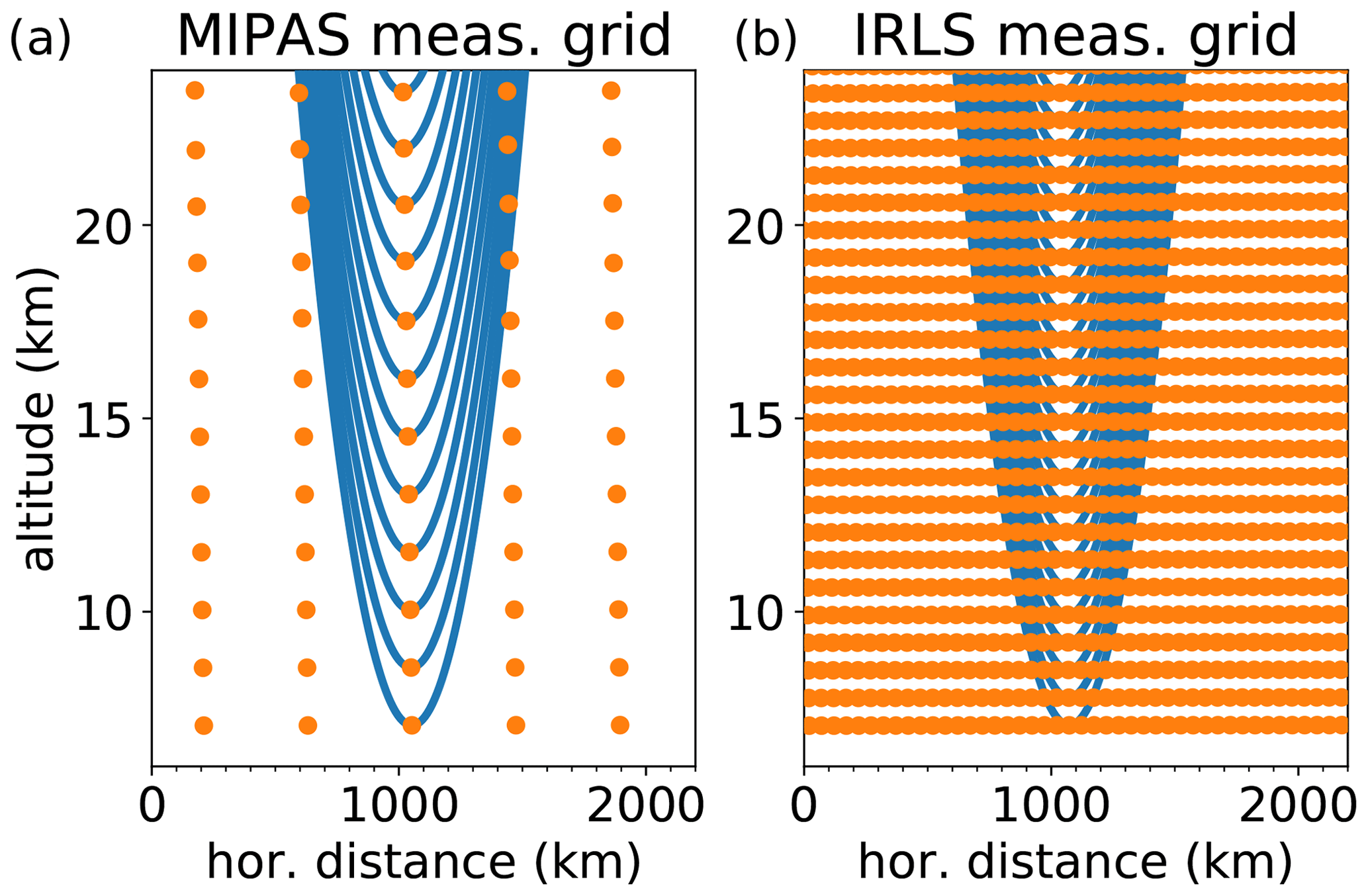
Figure 1 The measurement grid of a MIPAS-like instrument (a) and the IRLS (b). The blue lines indicate the lines of sight of single limb scans. The orange dots indicate the tangent points of multiple adjacent profiles 2100 km along track.

The first proposed spatial detection method is a two-dimensional evolution of the CI method, described in Sect. 3.3.1. The cloud detection is improved by taking into account not only the tangent point of a measurement but instead the full extent of and overlap within the tangent point layer. This extension already allows for the exploitation of the increased sampling density of IRLS-like instruments.

In addition, a much more computationally involved method is proposed in Sect. 3.3.2. This method deduces the atmospheric extinction values of clouds in a tomographic nonlinear inversion that has so far been mostly used to derive temperature and trace gas concentrations.

3.3.1 2-D convex hull CI

If the cloud index of a measurement is below the threshold, a cloud has been detected along the line of sight of the measurement. But it is not clear where along the measurement the cloud is located. It could be, in theory, in low Earth orbit, right in front of the satellite, close to the tangent point, or at any point in between or beyond. As such, the cloud index is better suited for selecting cloud-free measurements for trace gas retrievals than locating clouds. Due to the curvature of the Earth, the line of sight of a measurement stays longer in the atmospheric layer surrounding the tangent point than the layers above. This makes it more sensitive to clouds in this layer than the layers above; but the signal of a “thicker” cloud at a higher layer is still indistinguishable from a signal of a “thinner” cloud in the tangent layer.

This section introduces a method that exploits the existing overlap of measurements of limb sounder instruments to address this problem and improve upon the positioning of detected clouds, i.e., to properly compute the convex hull of clouds determined by the CI of individual spectra. The convex hull of a set of points is the smallest convex shape that fully encloses the points. As the CI is computed from integrated microwindows over a rather large spectral range, there is no meaningful effect on the results by the spectral resolutions of IRLS measurements. Therefore, this aspect of the different instruments is neglected. (Further, the increased spectral resolution typically comes at the cost of a reduced horizontal sampling, which counteracts the purpose of exploring the spatial detection capabilities.)

A common approximation of the spatial origin of a radiance measurement is assigning it to its tangent point, which is the location along its line of sight that is closest to the surface. This is the location where the air is densest and thus from where most radiation is emitted in optically thin conditions. Obviously, this assumption breaks down in the presence of clouds. This poses the largest problem in determining the position of clouds from the CI and the tangent point location alone. Figure 2 shows an extinction cross section and associated CI values. Comparing the location of small clouds (extinctions $>{\mathrm{10}}^{-\mathrm{3}}$ km⁻¹) in the upper panels to the corresponding structures in CI in the lower panels, one can easily see how the assumption of emission stemming from the tangent point breaks down for an optically thick (i.e., nontransparent) medium. The curved structures peak at the location of the cloud and then extend downwards to both sides for measurements that either “hit” the cloud before or after the tangent point. The resulting structure is still useful as it is a strict overestimate of the dimensions of the clouds (above the detection limit). Also the cloud top altitude of the true cloud can be properly determined to high accuracy compared to, e.g., nadir sounders.

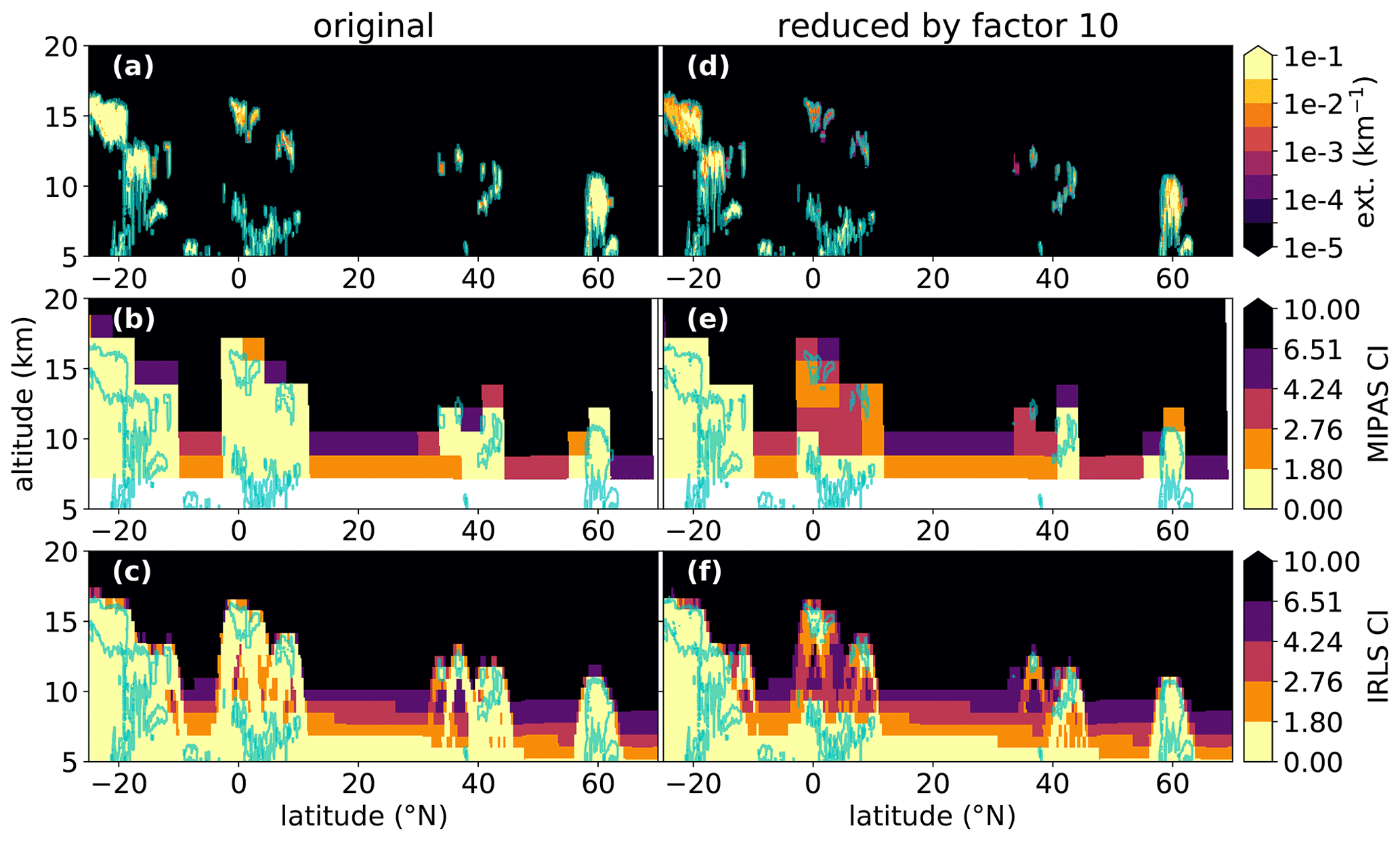
Figure 2 CALIOP extinction (a) and CALIOP extinction reduced by a factor of 10 (d) (measured on 1 December 2009 from 03:37:36 UTC onward) as well as the associated CI derived from simulated MIPAS measurements in (b, e). The CI derived from simulated IRLS measurements is given in (c, f), respectively. The contour line for an extinction value of 10⁻³ km⁻¹ is shown as a light blue line in all panels. The satellite looks northwards in these simulations.

Knowing that measurements indicated as cloud-free according to the CI typically have no cloud within the tangent point layer, where the lines of sight are nearly horizontal, we can improve the method. Especially optically thin ice clouds are often rather thin vertically, which means that the radiances measured by lines of sights passing through the thin cloud at steeper angles may not be strongly affected and thus not detect its presence. Therefore, one may not easily extend the cloud-free assumption to the layers that the line of sight passes through at altitudes significantly above the tangent altitude.

The proposed first new detection method works as follows:

• 1.

  Build a regular grid covering the cross section. Here, a grid with a vertical spacing of 500 m was chosen to be a bit finer than the measurement grid of the IRLS to be robust against slight variations of tangent point altitude due to temperature and pressure variations. The horizontal location of the profiles was taken to coincide with the lowermost tangent points (this causes a slight shift between grid and tangent point location for higher altitudes). Each grid box is assigned a value of 0 (i.e., it is assumed to be cloudy; final values of zero can also be used, however, to determine grid boxes without measurement information).

• 2.

  The line of sight for each spectrum is computed for a distance of d km before and behind its tangent point. Here, a very conservative (small) value of 100 km was chosen for d to reduce the number of false negatives (i.e., to decrease the number of undetected clouds).

• 3.

  Successively for each line of sight, each grid box that it passes through is assigned the maximum between its current value and the CI of the spectrum.

• 4.

  Lastly, the CI of each grid box is compared to the CI threshold associated with its altitude and latitude band (Sembhi et al., 2012) to determine whether or not a cloud is present.

This algorithm gives a cloud/no-cloud decision for the 2-D cross section measured by the limb sounder that is more precise than the CI method alone. For one cross section of a half-orbit as shown below (e.g., Fig. 4), the method uses less than 1 min of computation time on one core of an AMD EPYC 7351P 16 Core Processor operating at 2.9 GHz.

3.3.2 Tomographic extinction retrieval

The second method briefly investigates the capabilities of employing a full-blown nonlinear retrieval for the determination of cloud positions. This is a computationally more demanding task compared to the color-ratio-based schemes and as such may be less suited for a quick identification scheme for filtering affected spectra. However, computational capacity steadily increases, and the current scheme is well suited for real-time usage.

The method is comparable to the one employed by Castelli et al. (2011) but is simplified due to the neglect of scattering. The intent is to show the capabilities of this approach in combination with an increased measurement density. The retrieval employed the same JURASSIC2 forward model and setup that was used for generating the synthetic measurements. While the simulated measurements were generated using the original, fine grid on which the CALIOP L2 data are supplied, the retrieval grid was reduced to 500 m vertically in the relevant altitude range and ≈20 km horizontally. This corresponds to roughly 1000 profiles for the half-orbit in the CALIOP-based simulations. We use the same spectral setup as used for the generation of synthetic radiances; i.e., only two averaged radiances were simulated, centered at 792.00 and 833.00 cm⁻¹. The same trace gases and volume mixing ratios were used in the retrieval as in the forward simulation. Perfect knowledge was assumed for all trace gases, which is obviously a strong simplification. But due to the strong radiative effect even of thin ice clouds in the limb, this is likely justified, but its examination is beyond the scope of this study. Temperature and extinctions were assumed unknown, and climatological values and a zero profile were used as a priori information and initial guess for temperature and extinction, respectively. Also, the scattering effect of clouds was neglected here, as we are only interested in the detection, not in a quantitative analysis of the retrieved extinction.

Computing the spatially located extinction from the radiances poses an inverse problem. The solution to this problem is identified by iteratively modifying an atmospheric state x_i, i∈ℕ₀, such that the simulated measurements F(x_i) progressively agree better with the actual (in this case also partially simulated) measurements y within expectation of the noise equivalent spectral radiances (NESRs) of the measurements, under the side condition of being close to a “plausible” atmospheric state x_a:

$$\begin{array}{}\text{(1)}& \begin{array}{rl}{\mathit{x}}_{i+\mathrm{1}}=& {\mathit{x}}_i-{\left({\mathbf{S}}_{\mathrm{a}}^{-\mathrm{1}}+\mathbf{F}{}^{\prime }\left({\mathit{x}}_i{)}^{\mathrm{T}}{\mathbf{S}}_{\mathit{ϵ}}^{-\mathrm{1}}\mathbf{F}{}^{\prime }\right({\mathit{x}}_i)+{\mathit{\lambda }}_i{\mathbf{I}}_n\right)}^{-\mathrm{1}}\\ & \cdot \left({\mathbf{S}}_{\mathrm{a}}^{-\mathrm{1}}({\mathit{x}}_i-{\mathit{x}}_{\mathrm{a}})+\mathbf{F}{}^{\prime }({\mathit{x}}_i{)}^{\mathrm{T}}{\mathbf{S}}_{\mathit{ϵ}}^{-\mathrm{1}}\left(\mathit{F}\left({\mathit{x}}_i\right)-\mathit{y}\right)\right).\end{array}\end{array}$$

The matrix ${\mathbf{S}}_{\mathrm{a}}^{-\mathrm{1}}$ is defined as a Tikhonov–Phillips-type regularization matrix, imposing smoothness conditions in horizontal and vertical direction on the solution (Tikhonov and Arsenin, 1977). The parameter λ is a dampening parameter of the Levenberg–Marquardt algorithm and typically converges to zero as x_i converges on the solution (Levenberg, 1944). F^′(x_i) denotes the Jacobian matrix of F evaluated at x_i. Typically, one uses x_a as a value for x₀. The matrix S_ϵ is set up assuming a 0.1 % error in radiance, which has been chosen to allow for differences caused by the use of different grids for generating the synthetic measurements and the retrieval itself.

For temperature, only the second derivatives are constrained with correlation lengths of 1 km vertically and 200 km horizontally. Restraining the second derivative enforces a smooth lapse rate for temperature (Ungermann et al., 2015), which is useful for further analysis of the dynamical structure around the thermal tropopause. For extinction, the first derivatives in both spatial directions are constrained using the same correlation lengths in addition to imposing a weak constraint of the absolute extinction values towards the zero profile. These values are selected to be similar to those practically used in tomographic studies for the GLORIA instrument. The qualitative result does not depend largely on the type of regularization as long as it is neither too strong to smooth the solution nor too weak to allow for oscillations, as the aim is so far not to perfectly reproduce the original extinction values but to arrive at a simple cloud/no-cloud product. The retrieval employs the numerical techniques developed for the GLORIA limb sounder tomography to quickly derive a solution (Ungermann et al., 2010, 2011). As only two spectrally averaged samples are simulated from each spectrum, the computation time and memory consumption are manageable. The retrieval for a half-orbit consumes about 200 MB, mostly for storing Jacobian matrices, and requires about 25 min on eight cores (same machine as above) to converge to a satisfactory state, which can be readily accomplished in real time. A full day of measurements (for an exemplary 14.5 orbits) would thus consume ≈6 h.

4 Study on synthetic data

In this section we use synthetic spectra generated by JURASSIC2 based on CALIOP extinctions to evaluate the algorithms. To focus on the relative capabilities of the algorithms, we added Gaussian noise to simulated MIPAS or IRLS measurements with a standard deviation of 0.8 $\mathrm{nW}{\mathrm{cm}}^{-\mathrm{2}}{\mathrm{sr}}^{-\mathrm{1}}\mathrm{cm}$.

4.1 2-D convex hull CI

In a first step, we compare the cloud indices as gained from MIPAS-like and IRLS spectra. Figure 2b shows the CI for the simulated spectra based on an exemplary CALIOP cross section and the MIPAS measurement grid and spectral resolution. The simulated radiances were generated using the grid defined by the CALIOP L2 data shown in Fig. 2a. The “pixels” corresponding to MIPAS measurements in Fig. 2b are very coarse compared to the fine structure of the clouds contained in the CALIOP data due to the much sparser horizontal sampling density of the MIPAS instrument. Figure 2c shows the IRLS simulations. The increased spatial sampling density results in a much finer sampling of the clouds, but the bow-like artifacts due to the optically thick atmospheric conditions become apparent. These are also given in the synthetic MIPAS data but are barely discernible due to the coarse measurement grid. Figures 2d–f show the same situation but with CALIOP extinction reduced by a factor of 10. These numerical experiments shift the focus to very thin clouds that may not be present in the original data set.

The results of the convex hull CI algorithm are exemplarily depicted in Figs. 3 and 4. Figure 3 shows the results for the MIPAS instrument, while Fig. 4 shows the result for the IRLS instrument. For MIPAS, no obvious differences between CI and the convex hull CI are apparent. The minor visible discrepancies can be attributed to the difference between the tangent point grid of the CI and the rectilinear grid on which the convex hull CI algorithm operates. In contrast, a noticeable improvement can be seen for the IRLS measurements. The convex hull CI algorithm reduces the bow-like structures around thin clouds. Especially the comparatively small structures at 38^∘ N have a much reduced size, more aligned with the true structure as shown by the extinction contour. But a deficit is also apparent. Below thick clouds, no actual measurement information is present, and the CI is (wrongly) attributed to the tangent point location. This will still cause an overestimation of cloud presence.

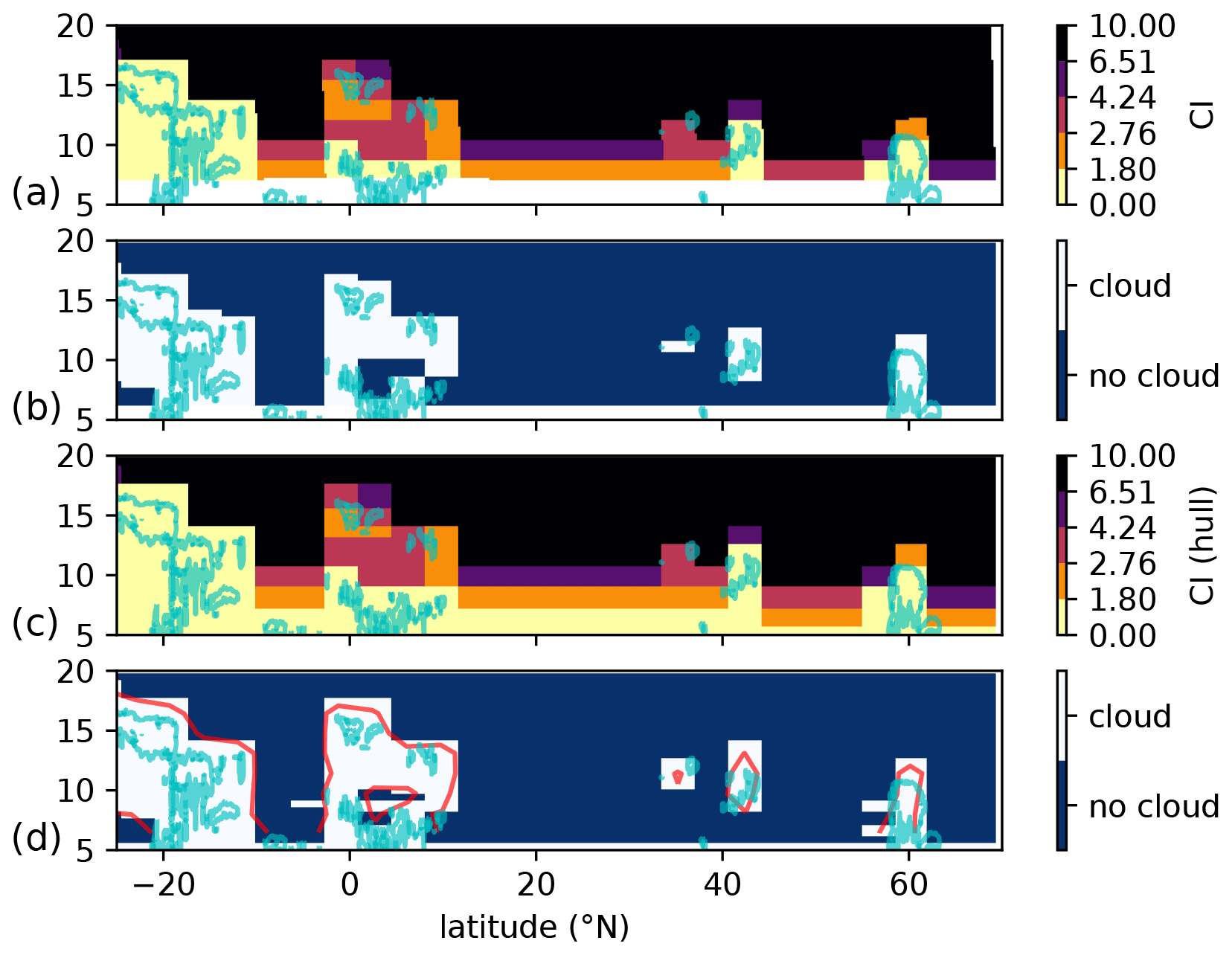
Figure 3 Result of the convex hull CI algorithm for MIPAS simulations based on CALIOP extinctions reduced by a factor of 10. Panel (a) shows the CI at the location of tangent points. Panel (b) shows the location of clouds according to the altitude dependent CI threshold. Panel (c) shows the CI determined with the convex hull CI algorithm. Panel (d) shows the location of clouds according to the altitude-dependent CI threshold. The cloud position from (b) is shown as a red contour line for reference. The contour line for a “true” extinction value of 10⁻³ km⁻¹ is shown as a light blue line in all panels. The satellite looks northwards in these simulations.

Figure 4 Result of the convex hull CI algorithm for IRLS simulations based on CALIOP extinctions reduced by a factor of 10. Panel (a) shows the CI at the location of the tangent points. Panel (b) shows the location of clouds according to the altitude-dependent CI threshold. Panel (c) shows the CI determined with the convex hull CI algorithm. Panel (d) shows the location of clouds according to the altitude-dependent CI threshold. The cloud position from (b) is shown as a red contour line for reference. The contour line for a “true” extinction value of 10⁻³ km⁻¹ is shown as a light blue line in all panels. The satellite looks northwards in these simulations.

4.2 2-D tomographic extinction retrieval

This section presents some results of the extinction retrieval. Figure 5 shows the extinction retrieved for the same extinction distribution derived from CALIOP data for MIPAS and IRLS data for one of the 440 processed cross sections. Both retrievals were set up identically with the difference that Fig. 5b used simulated MIPAS measurements and a coarser horizontal retrieval grid (≈160 km) and Fig. 5c used simulated IRLS measurements. The MIPAS-based retrieval is both horizontally and vertically coarser in comparison to the IRLS retrieval as required by the different measurement grid. The results are generally more accurate than the picture provided by the CI in Fig. 3 as even for the coarse MIPAS measurement grid, the overlap of measurements at higher altitudes can be used to constrain the location of thin clouds better. The retrieval using the IRLS measurement specification in Fig. 5c offers a much better resolved result. The finer spatial sampling and the reduced field of view allow us to see below clouds with clear-sky conditions, as with the equatorial high cirrus cloud. We also encountered similar conditions with our airborne instruments GLORIA (see below) and CRISTA-NF (Spang et al., 2008). The location of clouds, expressed in increased values of extinction, is more precise and much closer to the actual extinction distribution compared to the CI-based methods. Some artifacts remain below thick clouds, where, due to their opacity, no or nearly no measurement information is present. As such, the values below 9 km at 20^∘ S are not reliable. On the other hand, the weak structures at and above 15 km are well reproduced. Obviously, the retrieval works better for optically thin conditions.

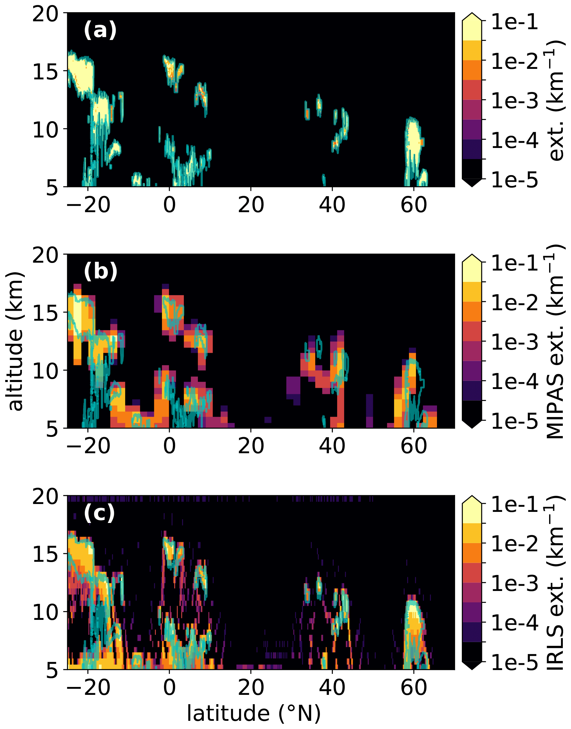
Figure 5 Retrieval of extinction from simulated measurements using CALIOP extinctions reduced by a factor of 10. Panel (a) shows the true extinction while Panel (b) shows the retrieved values for a MIPAS-like instrument. Panel (c) gives the results for an instrument with higher measurement density such as the IRLS. The contour line for a “true” extinction value of 10⁻³ km⁻¹ is shown as a light blue line in all panels. The satellite looks northwards in these simulations.

4.3 Comparison of 2-D cloud top detection accuracy

This section aims to quantify the performance of the 2-D convex hull CI and the 2-D tomographic extinction retrieval algorithms with respect to cloud top height estimation. We focus here on the capabilities of the IRLS instrument. Figure 6 shows an exemplary CALIOP orbit with detected cloud extent according to the CALIOP extinctions (extinction larger than 10⁻⁴ km⁻¹), cloud index (CI), convex hull cloud index (convex hull CI), and tomographic extinction retrieval (extinction larger than $\mathrm{3}\times {\mathrm{10}}^{-\mathrm{4}}$ km⁻¹). A slightly larger threshold is employed here, as the smoothing by the regularization extends the rather large extinctions vertically, and a smaller threshold would thus lead to a systematic overestimation of cloud extent. One can immediately see that all methods typically agree within about 1 km, with larger errors occurring at the border of extended cloud regions.

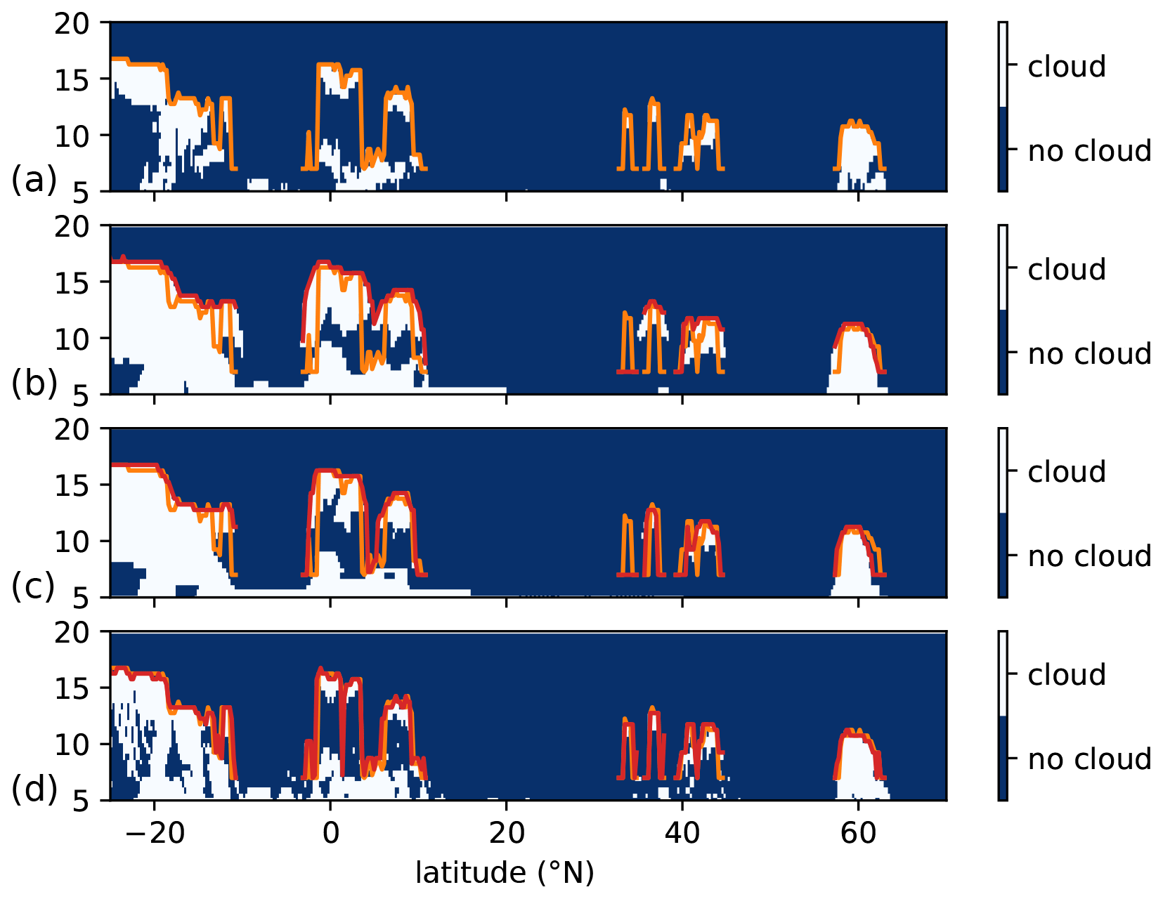
Figure 6 Comparison of cloud top detection capability for the various discussed methods and the IRLS instrument. Panel (a) shows the cloud extent contained in the CALIOP data. Panel (b) shows the cloud extent according to the CI. Panel (c) shows the cloud extent according to the convex hull CI algorithm. Panel (d) shows the cloud extent according to the tomographic extinction retrieval. In all panels, the orange line shows the true cloud top altitude, where clouds are present above 7 km with a lower limit of 7 km. The red line shows the cloud top altitude according to the depicted algorithm. The satellite looks northwards in these simulations.

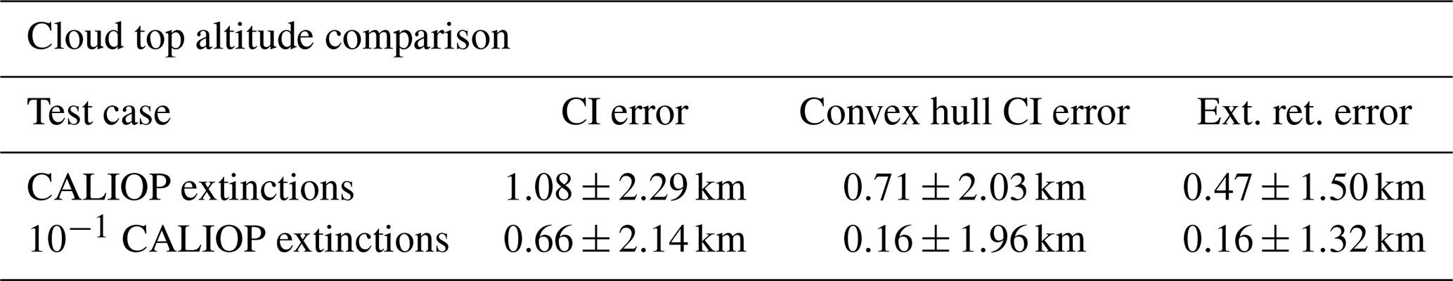
Table 1 shows the numerical results for the cloud top height derived by the three algorithms for 440 semi-randomly selected CALIOP orbits (we arbitrarily picked 1 month of data). Using unmodified CALIOP extinctions, the CI shows a positive bias of 1.08 km with a standard deviation of 2.29 km. There are two major sources for a high bias. First, the field of view of the instrument causes an overestimation of cloud top altitude, especially for thicker clouds (e.g., Griessbach et al., 2020a). Second, and more importantly, the cloud is horizontally extended, causing cloud detection events beside the actual cloud, where no cloud is in the original data (e.g., Kent et al., 1997). The second effect mainly causes the large variance in the results. As expected, the convex hull CI algorithm significantly reduces this bias, whereby the tomographic extinction retrieval even seems to be superior. Both are capable of reducing the impact of “horizontal cloud lengthening”. For thinner clouds, the situation improves all around. Using clouds that are an order of magnitude thinner, here, the CI shows a bias of only 0.66 km. For optically thinner clouds the general cloud top height overestimation is reduced or even turns into an underestimation (Griessbach et al., 2020a), and the horizontal cloud lengthening is also reduced (Fig. 5). The bias of the convex hull CI algorithm and the tomographic extinction retrieval are both on the order of 160 m, whereby the extinction retrieval has a reduced standard deviation compared to the convex hull algorithm.

Table 1 This table aggregates the difference between true cloud top altitude and determined cloud top altitude for 440 CALIOP orbits acquired in December 2012 for simulated IRLS measurements.

As the overestimation of the horizontal extent of clouds strongly affects the cloud top altitude comparison, we examined more closely how well the shape of the cloud top is reproduced. In a first step the true cloud top is determined from CALIOP extinctions. Using the tomographic extinction retrieval grid, all cloud top grid boxes plus all boxes within two squares' distance (Manhattan norm, ±1 km vertically, ±50 km horizontally) are selected for comparison. The results are collected in Table 2. The table shows an increase for correctly identified cloudy pixels for the three methods, with the conventional CI being worst and the tomographic extinction retrieval being best. False positives decrease accordingly. However, there is a slight increase for false negatives, which is caused by horizontally small clouds that are filtered away by the convex hull CI as the CI is pushed below the threshold and for which the tomographic extinction retrieval determines an extinction below the threshold (potentially due to slightly smearing out the cloud). This is confirmed by the numbers for the scaled extinction test cases, for which the number of false negatives increases across the board.

Table 2 This table aggregates the difference between the true cloud top shape and determined cloud top shape for 440 CALIOP orbits acquired in December 2012 for simulated IRLS measurements. All values are in percent.

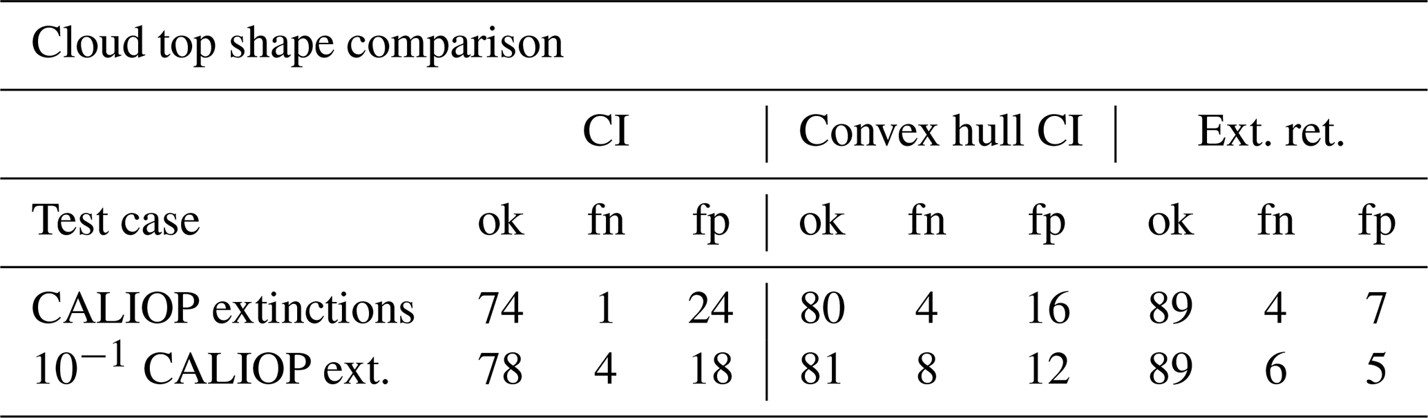
The label “ok” means correctly detected, “fn” false negative, and “fp” false positive.

4.4 3-D IRLS scenario – spatial detection capabilities

This section describes the result for the convex hull algorithm CI for the CLaMS-ICE-model-based simulations that allow for the simulation of the across-track coverage of the IRLS instrument in contrast to the CALIOP-based simulations that allow for only a simulation of the center track.

Figure 7 shows horizontal cross sections at several pressure levels through the extinctions derived from the 3-D CLaMS-ICE ice water content simulation. The center of the simulated IRLS measurements follows the 19^∘ W meridian. Actual satellite measurements of the instrument will not follow a perfect polar orbit, but for the simulations, the difference is negligible and simplifies the simulation setup. One can see a cloud field on the left-hand side on lower altitudes and a second cloud field on the right-hand side at different altitudes. At higher latitudes, the two cloud fields merge. This situation gives a nice across-track variation over the images of the IRLS that can be examined in the following.

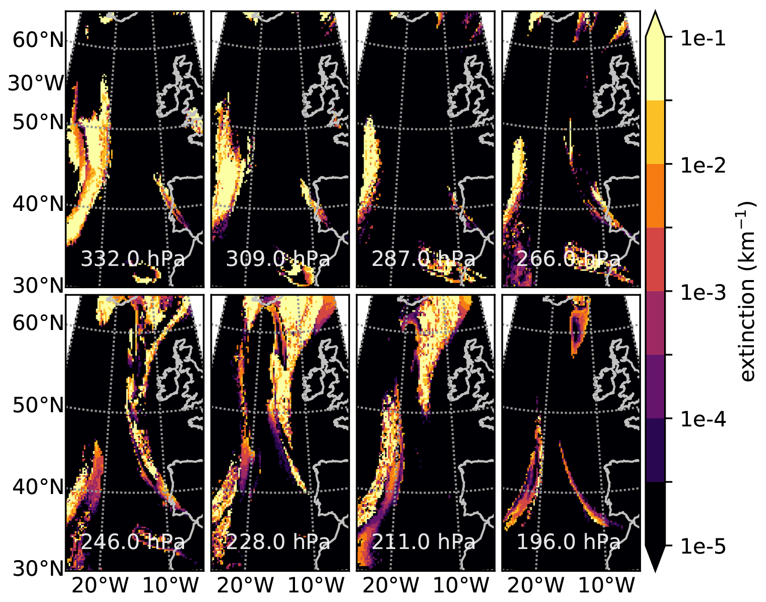
Figure 7 Extinction of a cirrus cloud simulated by CLaMS-ICE and computed from ice water content and particle radii.

This variation can be seen better in Fig. 8 that shows the CLaMS-ICE extinction as “images” as the IRLS would see them. Each “pixel” of the picture corresponds to one pixel of the IRLS, but the horizontal coverage is slightly larger by 2 pixels. The IRLS would take roughly twice as many images of the situation than depicted here. The depicted images cover the latitudes from 39.1 to 64.6^∘ N. The simulation ends shortly beyond these latitudes. The images show a two-layered structure on the left-hand side between 42.7 and 51.9^∘ N. Northward of 46.4^∘ N, one can see the second cloud structure to the right, first with rather faint extinctions and then higher ones until the two structures join around 61^∘ N.

Figure 8 Cross section through CLaMS-ICE extinction data corresponding roughly to the field of view of the IRLS. Only every second image of the IRLS is depicted.

The measurements of the individual tracks can be treated individually as singular cross sections and may be assembled in a second step. As MIPAS only measured a single track, no MIPAS simulations are shown here for comparison as the results will not be different from those of Sect. 4.1.

The computation of the conventional CI and the application of the cloud index threshold are depicted in Fig. 9a and b. Similar to the simulations of Sect. 4.1, the cloud extent is overestimated to the sides of the clouds and below. The result of the convex hull CI algorithm is shown in Fig. 9c and d. One can see again that the new algorithm follows the true extinction more closely. In the case of the central track (Fig. 9e), it becomes apparent that the chosen value for extinction of 10⁻³ km⁻¹ is not the true detection limit as the faint cloud structure in the center track below that limit is also detected by the CI.

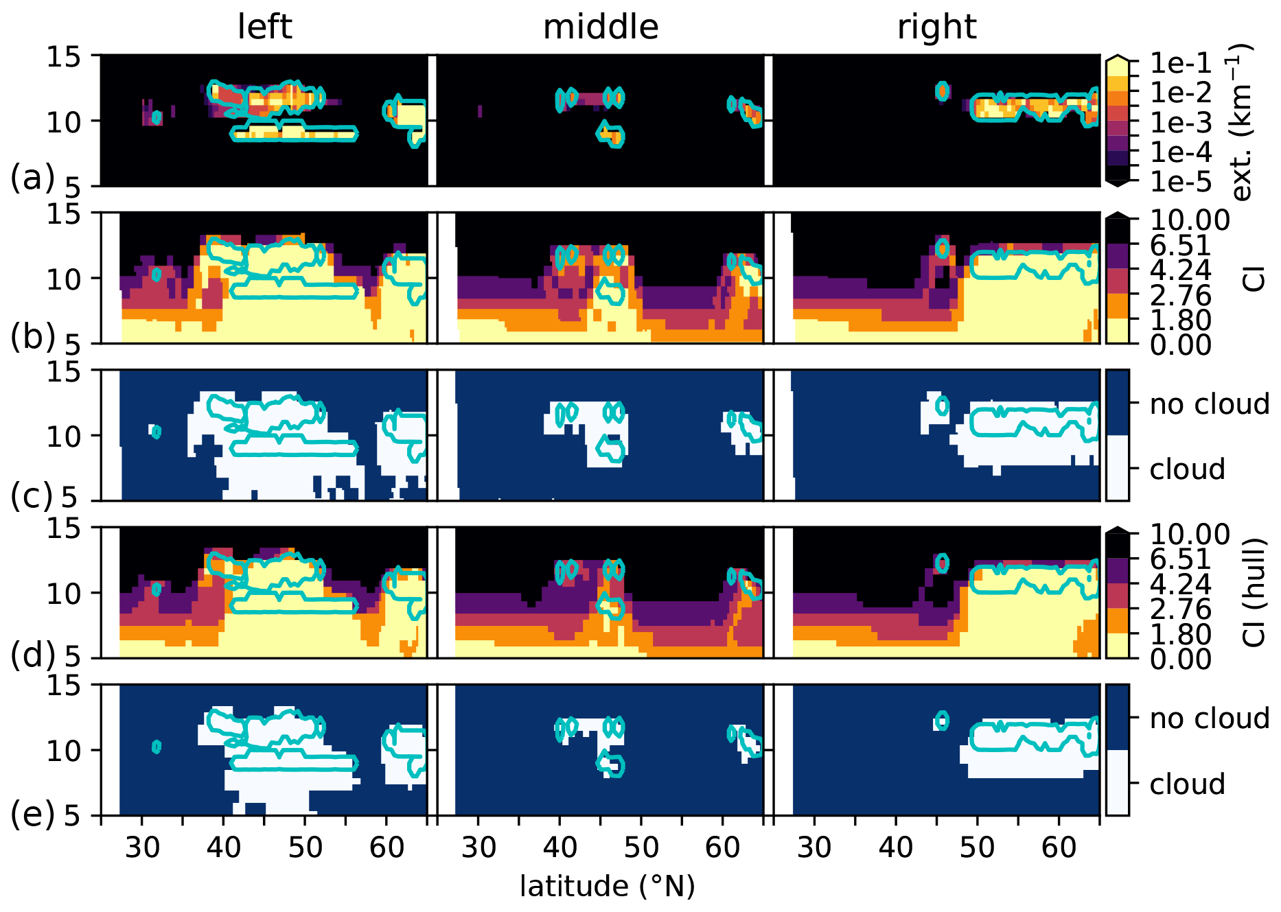
Figure 9 Cloud index and convex hull CI for three measurement tracks of a simulated IRLS instrument (left, center, and right). Panel (a) shows the extinction values used for generating the simulated measurements. Panel (b) shows the cloud index, and (c) shows the corresponding cloud detection. Panel (d) shows the CI as derived from the convex hull CI algorithm, whereas (e) shows the cloud detection for the convex hull CI. The contour line for a “true” extinction value of 10⁻³ km⁻¹ is shown as a light blue line in all panels.

The individual tracks can then be assembled into a three-dimensional view on the cloud structure. Figure 10a shows a three-dimensional representation of the true extinction distribution. The zonal extent is limited by the measurement coverage of the IRLS. One can see the across-track and along-track variation as well as the vertical structure. The result of the convex hull CI algorithm is presented in Fig. 10b. The three-dimensional results agree similarly to the cross sections discussed before. The cloud extent is slightly overestimated horizontally, and the vertical structure of the cloud is lost; the bottom of the cloud is often located lower than in the actual extinction structure. Also, the very small spot of a cloud to the south was not detected.

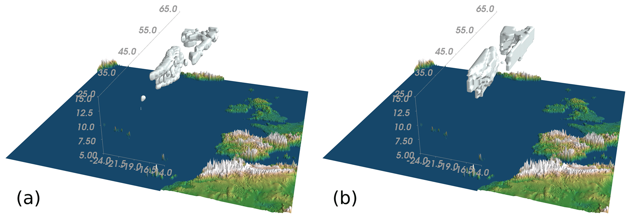
Figure 10 The true (a) and derived (b) cloud structure using the convex hull CI algorithm. A white contour surface is shown for 10⁻³ km⁻¹ in the measurement track of the IRLS. The vertical dimension is stretched by a factor of roughly 100. Due to the employed cylindrical projection, the measurements expand towards the back.

5 3-D retrievals using GLORIA measurements

The final section applies the extinction retrieval approach to real measurements. While currently no limb sounding satellite instrument with a sufficient measurement density in the UTLS exists, the airborne GLORIA instrument can serve well for a feasibility study, even though the 3-D retrieval of GLORIA is more complicated than the one needed for satellite-borne instruments. In fact, it resembles techniques to reconstruct 3-D cloud structures from ground-based cloud imagers more closely (Mejia et al., 2018) but with a horizontal viewing geometry and a moving single instrument instead of multiple stationary ones. We determine a spatially resolved extinction value that does not allow us to distinguish between trace gas, ice cloud, and aerosol emission. In the given spectral range, emission from trace gases is negligible compared to that of ice clouds, and we know from closer inspection of spectra and other sources of information that there was no strong aerosol load such as that generated by a volcanic eruption or biomass burning.

This numerical experiment uses measurements acquired on 18 September 2017 during the WISE campaign. Here, the GLORIA instrument operated with a spectral sampling of 0.2 cm⁻¹ and panning from 45 to 132^∘ in 6^∘ steps while following a straight flight path.

We used all images taken between 11:10 UTC and 12:35 UTC in the reconstruction. The 3-D retrieval is computationally significantly more expensive compared to the 2-D retrievals as the number of unknowns is much higher, and the algorithms involved scale with a power of given unknowns. The atmospheric volume is also much less constrained by the measurements as the number of unknowns vastly outnumbers the measurements, and the distribution of information is far from homogeneous. We found that deriving temperature and extinction similar to the 2-D setup works well within the volume covered by tangent points but quickly deteriorates outside. Thus, we neglect the temperature retrieval here, as this improved the retrieval on three fronts. First, this allows the 792 cm⁻¹ window to be discarded and any trace gas emissions to not be taken into account in the forward modeling, drastically improving the forward model speed by orders of magnitude. Second, it halved the number of unknowns, thereby increasing convergence speed of iterative solvers by a factor of roughly 4 and decreasing memory consumption by half. Third, this also stabilized the extinction retrieval such that the extinction values outside the core volume are less affected by retrieval artifacts. The single microwindow employed averaged all spectral samples between 831.2 and 835.0 cm⁻¹ (GLORIA operated in a mode that allows for a spectral sampling of 0.2 cm⁻¹ during this portion of the flight). Measurements with tangent points below ≈9 km altitude were discarded as they do not contribute to the reconstruction of the cirrus clouds at higher altitudes. Thus, 629 separate images with 61 611 radiance values in total were employed in the retrieval. Figure 11 shows one exemplary cloud scene. While the camera in the visible samples a viewing angle of about 11^∘ and shows an extended cirrus cloud at ≈10.5 km, the infrared camera only samples a section of about 1.5^∘. Here, the employed horizontal averaging over the IR pixels is useful, but other imaged clouds exhibit finer structures within an image, similar to the filament at 319.3^∘ azimuth. But, even with the fine retrieval grid described below, they would remain inaccessible. Future work will encompass a measurement scheme that reduces the horizontal gaps between images and exploits the full resolution capabilities of the detector.

Figure 11 A superposition of a visible and infrared image taken at 11:50:31 UTC, showing a cirrus cloud located at 10.5 km. The visible image has a much wider field of view than the infrared one. The infrared image has been extracted from the spectrally resolved GLORIA measurements and shows the averaged radiance over the spectral range from 831.2 to 835.0 cm⁻¹; it has also been shifted to the right for better comparability, and the radiance is depicted on a logarithmic scale with arbitrary units. The black frame marks the original position. The altitude axis on the right gives an approximate tangent point altitude.

The retrieval grid used a vertical sampling of 125 m and a horizontal sampling of 10 km in both horizontal directions. The grid is rectilinear in a stereographic projection centered around the center point of the volume rotated in such a fashion that one axis of the grid is parallel to the flight path. The grid covered the volume of ±1000 km in the horizontal direction and between 8 and 16 km altitude in the vertical direction. The grid was extended further to encompass the whole measured volume up to 64 km altitude at a reduced sampling¹. Altogether, this resulted in 3 235 925 extinction values to be reconstructed. This number is significantly larger than the number of measurements, making this a drastically underdetermined problem.

The inverse problem, i.e., identifying an atmospheric state fitting to the measurements, is an ill-posed problem. To solve it, we approximate it by a well-posed, regularized formulation. To regularize the problem, we employ constraints of zeroth and first order. We used a standard deviation for extinction of 10⁻³ km⁻¹ for atmospheric samples with an ECMWF potential vorticity (PV) below 3 PVU and $\mathrm{5}\times {\mathrm{10}}^{-\mathrm{5}}$ km⁻¹ for atmospheric samples with an ECMWF potential vorticity above 5 PVU. In between, a linearly interpolated value was used. This setup avoids strong cloud signals in the stratosphere, which might otherwise appear as artifacts outside the well-measured volume and it does not affect the reconstructed extinctions in the well-resolved region. We assumed extinction structures to be typically ≈100 times longer horizontally than vertically and scaled the first derivative accordingly. The well-resolved volume surrounds the locations of the tangent points and is highlighted in the retrieval results. See Krisch et al. (2018) for a more involved discussion on this kind of linear-flight tomography and its capabilities.

Figure 12 shows the measured brightness temperatures of the averaged microwindow used in the retrieval taken at different azimuth angles. Just these three given angles already give some insight into the real cloud structure (while the retrieval also has access to the full set of angles). The thin structure at 10.5 km at 11:45 UTC in Fig. 12a is the increased radiance emitted by a cirrus cloud. From this figure alone, it is not determined if the cloud extends vertically over several kilometers or moves away from the aircraft at earlier measurements. The images taken at different azimuth angles deliver the missing information. The image taken at 126^∘ shows the cloud shrunk to nearly a single blob. This tells us the angle of the elongated cirrus cloud with respect to the flight path. Taken together, we can compute that this cloud nearly runs in a perfect north–south direction. In combination with the slanted structure of the cloud at other angles, the horizontal extent orthogonal to the flight path can be computed. Further information could be discerned from the vertical structure at 11:45 UTC in Fig. 12b. A similar structure is given in all measurements taken at this time. This is caused by a cloud very close to the aircraft as it is seen at all azimuth angles around this same time but not present at times more than a couple of minutes before and after. The retrieval is a mathematical method to extract this and more information from the measurements in an optimal fashion.

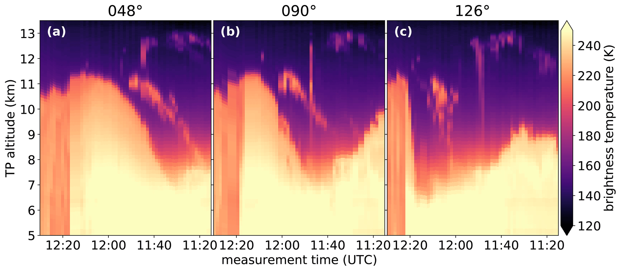
Figure 12 Brightness temperature of GLORIA measurements averaged over the wavenumber range from 831.2 to 835 cm⁻¹ (the same that is used as in the tomographic retrieval) over time, sorted according to azimuth angle in relation to aircraft heading.

The volume can best be reconstructed close to the tangent points of the radiance measurements (e.g., Krisch et al., 2018). Atmospheric samples much closer to the flight path were not measured at all. Atmospheric samples beyond the volume covered by tangent points could also be reconstructed but with quickly deteriorating quality. As in all tomographic reconstructions, measured structures are smeared along the lines of sight of the measurements if not constrained by measurements taken at different angles. Due to the curvature of the Earth, thick clouds measured at low altitudes are smeared along the line of sight, which curves upwards from the tangent points and causes high extinction values at implausible altitudes — which is one of the reasons we employed the PV-dependent regularization scheme. Please note that due to the geometry of satellite measurements, the overlap of the lines of sight is much better, which prevents such artifacts. The results of the reconstruction are depicted in Fig. 13. The two horizontal cross sections show retrieved extinction values at two altitudes. At 10.5 km, one can see two cloud structures close to Iceland, a vertically thick and horizontally extended cloud at 20^∘ W and the thin cirrus cloud previously discussed at 16^∘ W. The north–south extension already visible from Fig. 12 is also present here. Neither of the clouds visible at 10.5 km extends up to 12.5 km, where several small clouds close to the flight path are reproduced by the retrieval, which are associated with the vertically elongated areas of increased radiance in Fig. 12.

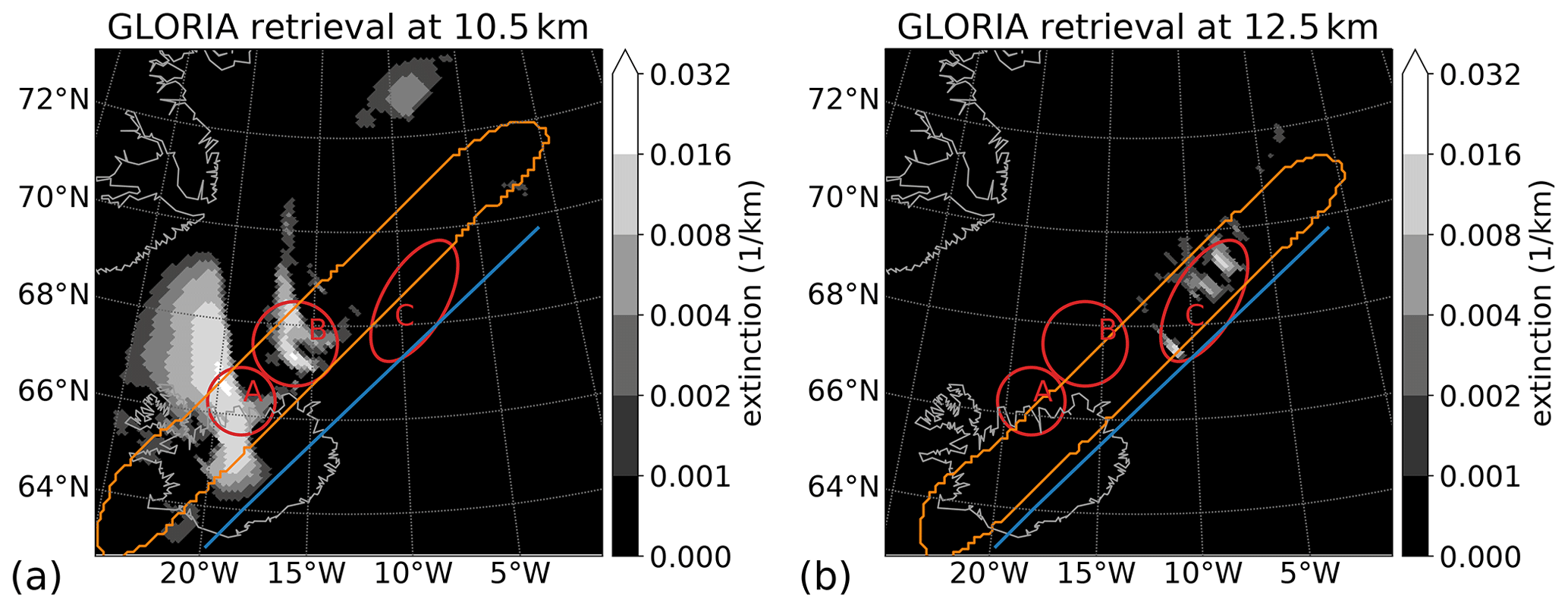
Figure 13 Cross sections of extinction retrieved from GLORIA measurements. Panel (a) shows a horizontal cross section at 10.5 km and (b) one at 12.5 km. The flight path is shown in blue; the trust region with high confidence in retrieval results around the tangent points of measurements is marked in orange. The three red ellipses mark areas of interest.

A theoretical analysis of the achieved resolution gives similar results to our previous work on deriving temperature structures (Krisch et al., 2018). Within the well-resolved volume the analysis shows an information content of about 0.05; i.e., 20 samples share about 1 degree of freedom; outside it drops to an order of magnitude less, but numerical instabilities of the involved equation systems make this difficult to compute precisely. Some systematic uncertainty due to uncertainty in the line of sight might bias the cloud tops' estimate². The vertical resolution in the area of the cirrus clouds is in the order of 300 m, decreasing to 400 m for lower levels. The horizontal resolution is on the order of 30 km in the flight-track direction and 70 km orthogonal to that. Circular flight patterns, or, better, a backwards-viewing limb satellite, could further improve the horizontal resolution (Ungermann et al., 2011; Krisch et al., 2017).

While the vertical extent, especially the cloud top, can be deduced with very high precision compared to nadir-viewing instruments, it is not obvious that the horizontal extent was properly derived. For verification and comparison of the quality of both, we used nadir-viewing images of the Spinning Enhanced Visible and Infrared Imager (SEVIRI; Schmetz et al., 2002) on the second-generation operational weather satellite Meteosat (MSG) and the Moderate Resolution Imaging Spectroradiometer (MODIS; Platnick et al., 2015, 2017) on the Terra satellite. Due to its geostationary orbit, SEVIRI offers a good temporal coverage. Two spectral channels are shown in Fig. 14. The image from the visible spectrum at 0.8 µm shows scattered light from clouds at all altitudes. The second channel at 12.0 µm shows the brightness temperature of infrared light emitted by the ground and clouds. (While scattering also plays a role here, we believe its influence to be small enough such that we can neglect it for this qualitative discussion.) The 12 µm channel was selected as it uses the same spectral region that is also used in the GLORIA extinction retrieval. Clouds at higher altitude have a smaller brightness temperature than clouds at lower altitudes due to their lower temperature. Both images were taken at 12:00 UTC, which corresponds roughly to the midpoint of GLORIA measurements. In addition, we used the cloud top product from the MODIS instrument that passed over our measurement area in low Earth orbit around 13:08 UTC, which is only slightly beyond GLORIA's measurement period and is still reasonably close to compare the cloud top altitudes. However, the horizontal position might have been shifted due to advection, and small clouds may also appear and disappear due to condensation and evaporation. Figure 15 shows the level 2 cloud top altitude product.

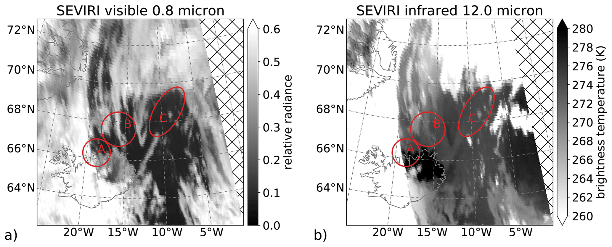
Figure 14 Two images taken by SEVIRI on Meteosat on 18 September 2017 at 12:00 UTC. Panel (a) shows the 0.8 µm visible channel in a relative scale, and (b) shows the 12.0 µm infrared channel as brightness temperature. The three red ellipses mark areas of interest. Hatched areas indicate missing data.

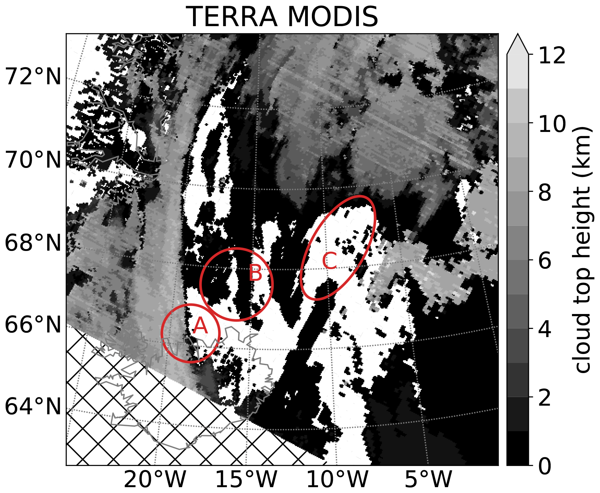
Figure 15 The cloud top altitude L2 product of MODIS on TERRA taken on 18th September 2017 around 13:08 UTC. White indicates no recognized cloud. The three red ellipses mark areas of interest. Hatched areas indicate missing data.

We focus first on region A in Figs. 13, 14, and 15. The GLORIA radiance and extinction data show here an optically thick cloud within the jet stream, vertically ranging over several kilometers and topping out at ≈11 km. This agrees with the MODIS cloud top data (mostly 10.5 km, with some pixels slightly above 11.0 km) and is also consistent with the low brightness temperatures (<260 K) in the SEVIRI 12 µm band. In the horizontal, both SEVIRI and MODIS see the high-altitude cloud in the same position, filling approximately the same area in region A and indicating no significant horizontal movement between both measurements. However, the GLORIA measurements fill a larger fraction of region A, which we attribute to the horizontal and temporal smearing of the retrieval (also, here, a fast-moving satellite would be subject to less temporal smearing due to a changing scene). The SEVIRI time series shows that the front is moving quickly eastwards, and the 12:15 UTC image agrees already much better with our data (please note that the images containing most information were taken around 12:22 UTC pointing at 126^∘ in relation to aircraft heading).

Second, we compare the structures found in region B in the same figures. There is a cloud stretching in a north–south direction for several hundreds of kilometers, with a brightness temperature of 272±1 K according to SEVIRI. The structure and location of the cloud visible in SEVIRI data compare favorably with a cloud located at the same horizontal position at 10 to 10.75 km altitude in the GLORIA extinction retrieval (only one layer is depicted in Fig. 13). The magnitude of derived extinction indicates that the cloud is quite transparent in the nadir view such that the brightness temperature of SEVIRI is certainly largely caused by warmer air and haze of lower altitudes. This cloud (≈1.5 km thick, with an extinction of ≈0.014 km⁻¹) hence should reduce the measured nadir brightness temperature by ≈1.3 K, which is roughly consistent with the difference of 1.5 K observed by SEVIRI between the cloud and surrounding air. Please note that the cirrus cloud is well visible in the optical regime in Fig. 11. In addition, MODIS sees quite a similar cloud but assigns it a cloud top altitude of below 1000 m, consistent with the high brightness temperature visible in SEVIRI. For these thin layers of cirrus, a limb sounder provides much higher accuracy in cloud top determination than state-of-the-art cloud top products derived from nadir sounders (Weisz et al., 2007).

Third, region C is discussed. In contrast to the other, larger clouds, GLORIA detected very small clouds, bringing it to its spatial detection limits, as these clouds are small enough to fall into the gaps of the horizontal scans. However, the measurements indicate very thin cirrus clouds at an altitude of 12 to 13 km. The retrieval assembles the measurements in a region with small, spotty clouds of differing optical thickness with a top altitude of 12.75 km, which coincides with the cold point tropopause having a temperature here of ≈210 K. While SEVIRI and MODIS show similar small patchy clouds in region C, it is more difficult to assign the high-altitude clouds retrieved from GLORIA. The cloud feature at the southern tip of region C agrees with a cloud feature measured by SEVIRI and MODIS. While the low brightness temperature of SEVIRI's 12 µm channel indicates a high-altitude cloud, as in region A, the MODIS cloud top altitude is below 2 km. From this discrepancy we deduce that these patchy clouds are probably too small and/or optically thin for IR nadir measurements to properly assign a cloud top altitude. While some of these have a comparably low brightness temperature of 265 K (the bright spot at the lowermost corner of region C), it is quite different from the 210 K corresponding to the altitude of the clouds detected by GLORIA. Due to the location close to the flight path, it could even be that the clouds that are visible in SEVIRI are unrelated clouds at lower altitudes as they would be outside the field of view of GLORIA. While the large cloud of region B was detected by MODIS, albeit at much too low an altitude, these even thinner clouds have likely been missed totally. There are no high clouds in the MODIS data in region C, and it is not easy to construct a relationship between the very small low clouds in region C in MODIS and our high clouds.

6 Conclusions

We presented a new cloud index product, the convex hull cloud index, which can exploit the higher measurement density of current and future oversampling limb sounders. While it cannot improve upon the cloud identification for older limb sounders such as MIPAS, it offers a significantly better cloud identification for higher measurement densities. We could show that it can properly locate clouds along the line of sight for many cases involving cirrus clouds and thus reduce the number of false positive cloud detection events by about 30 %. This method does not require a radiative transfer model and is computationally very cheap.

In addition, we introduced a tomographic extinction retrieval for cloud detection based on recent advances in retrieval techniques for limb sounders. The method uses the same algorithms and models used for 3-D temperature and trace gas reconstructions. In its current state, the required computational time is small compared to the measurement time, thus allowing for real-time application. The tomographic extinction retrieval generated a statistically better result compared to the color ratio methods, with a reduction of false positive detection events of more than 60 % compared to the standard cloud index. It excels in optically thin conditions but could deal well with all typical cirrus clouds in the upper troposphere. For optically thick conditions present at lower altitudes, the algorithms are naturally limited by the lack of information on the measurements by the limb sounders. Here, synergy with available nadir sounders could be exploited.

We finally applied the extinction retrieval to real measurements by the GLORIA limb sounder and could reconstruct several high- and low-altitude clouds in three dimensions. The vertical and horizontal position of these clouds were compared to images of the SEVIRI instrument and the cloud top altitude product based on MODIS data. We found good agreement in the general structure of the detected thick cirrus clouds. For thinner cirrus clouds, horizontal extent agreed, but vertical positioning disagreed. For very small and high cirrus clouds, no strong correlation was found between the three products. Determining the cloud top altitude of the reconstructed clouds from GLORIA measurements is easily feasible, with an accuracy of less than 300 m, while the horizontal positioning is less certain. Due to the tomographic measurement principle, a resolution of 30 to 70 km can be achieved, which may be further worsened depending on advection due to strong winds.

In summary, we have shown that tomographic reconstruction schemes applied to densely sampled limb sounding observations allow a wealth of information to be extracted on high clouds, reaching beyond what standard methods can achieve. It demonstrates that these kind of observations are well suited to collect information on high clouds which are not accessible by other kinds of global measurements.