Estimation of cloud optical thickness, single scattering albedo and effective droplet radius using a shortwave radiative closure study in Payerne

We have used a method based on ground-based solar radiation measurements and radiative transfer models (RTMs) in order to estimate the following cloud optical properties: cloud optical thickness (COT), cloud single scattering albedo (SSAc) and effective droplet radius (r_eff). The method is based on the minimisation of the difference between modelled and measured downward shortwave radiation (DSR). The optical properties are estimated for more than 3000 stratus–altostratus (St–As) and 206 cirrus–cirrostratus (Ci–Cs) measurements during 2013–2017, at the Baseline Surface Radiation Network (BSRN) station in Payerne, Switzerland. The RTM libRadtran is used to simulate the total DSR as well as its direct and diffuse components. The model inputs of additional atmospheric parameters are either ground- or satellite-based measurements. The cloud cases are identified by the use of an all-sky cloud camera. For the low- to mid-level cloud class St–As, 95 % of the estimated cloud optical thickness values using total DSR measurements in combination with a RTM, herein abbreviated as COT_DSR, are between 12 and 92 with a geometric mean and standard deviation of 33.8 and 1.7, respectively. The comparison of these COT_DSR values with COT_Barnard values retrieved from an independent empirical equation results in a mean difference of $-\mathrm{1.2}\pm \mathrm{2.7}$ and is thus within the method uncertainty. However, there is a larger mean difference of around 18 between COT_DSR and COT values derived from MODIS level-2 (L2), Collection 6.1 (C6.1) data (COT_MODIS). The estimated r_eff (from liquid water path and COT_DSR) for St–As are between 2 and 20 µm. For the high-level cloud class Ci–Cs, COT_DSR is derived considering the direct radiation, and 95 % of the COT_DSR values are between 0.32 and 1.40. For Ci–Cs, 95 % of the SSAc values are estimated to be between 0.84 and 0.99 using the diffuse radiation. The COT for Ci–Cs is also estimated from data from precision filter radiometers (PFRs) at various wavelengths (COT_PFR). The herein presented method could be applied and validated at other stations with direct and diffuse radiation measurements.

1 Introduction

Clouds are a major component of the climate system and have a significant influence on the Earth's radiation budget (Boucher et al., 2013). Cloud optical thickness (COT) is a key parameter of the cloud optical properties, which in turn are of interest for determination of the cloud radiative effect (Jensen et al., 1994; Chen et al., 2000; Baran, 2009; Hong and Liu, 2015). The radiative or optical properties of clouds are determined by their macrophysical and microphysical properties. The accurate parametrisation of these optical properties in climate models is a challenge because the small-scale physical processes of clouds are difficult to explicitly represent in global climate models (e.g. Waliser et al., 2009; Baran, 2012; Taylor, 2012; Zelinka et al., 2013; Ceppi et al., 2017). Thus, the introduction of methodologies using long-term observation aiming at the improvement of COT retrieval are important for estimations of the magnitude of the influence of the diverse and variable cloud situations on the climate system.

A common practice to determine COT values is with the use of satellite-based instruments and the so-called bi-spectral method (Nakajima and King, 1990; Platnick et al., 2017). Although this approach has shown good results on a global scale, there are also a number of potential uncertainty sources, namely in the spectral radiation calibration, horizontal and vertical inhomogeneities and inappropriate use of cloud microphysics (Zeng et al., 2012). In addition, satellite-based lidar systems such as the Cloud-Aerosol Lidar with Orthogonal Polarization (CALIOP) provide high-resolution vertical profiles of clouds (Winker et al., 2009), including products such as cloud extinction and backscatter profiles (Amiridis et al., 2015). Other studies describe a COT retrieval method from satellites using neural-network-based approaches (Kox et al., 2014; Minnis et al., 2016).

Cloud optical properties can also be estimated from airborne measurements (e.g. Finger et al., 2016; Krisna et al., 2018). Flying directly below or above clouds allows both accurate measurements and direct comparisons and validations of the COT values retrieved from satellite sensors. However, these campaigns are cost-intensive and thus the spatial and temporal resolution of data is poor.

A number of studies have presented methods for the retrieval of COT using data from ground-based instruments, for example, from lidars (Gouveia et al., 2017), broadband pyranometers (Leontyeva and Stamnes, 1994; Barnard and Long, 2004; Qiu, 2006), sunphotometers (Min and Harrison, 1996; Chiu et al., 2010) or UV radiometers (Serrano et al., 2014). With ground-based microwave instruments the liquid water path (LWP) is determined (Dupont et al., 2018), which can be used to calculate the cloud optical thickness, knowing or assuming r_eff (Stephens, 1994). An advantage of surface-based determinations of COT in comparison to satellite-based retrieval is that transmitted radiation is less sensitive to uncertainties in cloud droplet-size distributions than reflected radiation (Rawlins and Foot, 1990). Ground-based and airborne retrieval methods can be combined in order to achieve more accurate results for COT retrieval (Schäfer et al., 2018). Chiu et al. (2010) compared COT values retrieved from a sunphotometer with Moderate Resolution Imaging Spectroradiometer (MODIS) level-2 (L2) data with reasonable results in the COT agreement in a few cases. In order to compare COT retrievals on a global scale, networks with large global coverage and density as well as easily accessible data are needed. Barnard and Long (2004) showed a first approach in this direction by using only broadband diffuse shortwave radiation, surface albedo, solar zenith angle (SZA) and a clear-sky model in order to estimate COT. Matamoros et al. (2011) presented another empirical equation to estimate COT from the atmospheric transmittance at 415 nm, SZA, surface albedo, r_eff and aerosol optical depth (AOD). It has been proven that both empirical equations can be used for homogeneous low-level clouds (COT >10) but not for high-level clouds. The aim of our study is to use a method which is based on a radiative closure study and which allows the determination of COT independent of the cloud level.

In principle, radiative closure studies assess the difference between modelled and measured shortwave or longwave radiation. Among other things they allow estimation of the importance of accurate input variables and can be used to evaluate the accuracy of the retrieval of cloud optical properties (Wang et al., 2011). Nowak et al. (2008b) pointed out that in most cloud cases, radiative closure can only be achieved by having information about the cloud microphysical properties. This because e.g. stratus nebulosus can have large variations in cloud extent, cloud droplet concentrations, optical thickness and liquid water path (Dong et al., 2000).

With data from an airborne measurement campaign, Ackerman et al. (2003) achieved an agreement in the total shortwave radiation of within 8 % to 14 % for three single-layered stratus cases only by iteratively determining r_eff. McFarlane and Evans (2004) presented a study where they included r_eff and liquid water content (LWC) from microwave and cloud radar measurements in the model resulting in a difference of 10 % between simulated and measured total downward shortwave radiation (DSR). Nevertheless, this fairly good agreement was only achieved after averaging the data over a time period of 60 min. Nowak et al. (2008b) achieved an agreement between the modelled and observed shortwave radiation within measurement uncertainty in one-third of 32 selected and well-defined stratus nebulosus cases without adjusting any cloud properties. For the other cases, the cloud vertical extinction had to be adjusted in order to obtain an agreement within instrumental uncertainty. Wang et al. (2011) found a mean difference to within 5 % ±13 % for shortwave radiation for more than 600 well-defined thick low-level cloud cases at the Baseline Surface Radiation Network (BSRN) site Cabauw. They calculated COT according to the formula from Stephens (1994) using r_eff from MODIS data and LWP from a ground-based microwave instrument.

In the current study we estimate cloud optical thickness for stratus–altostratus (St–As) and cirrus–cirrostratus (Ci–Cs) using broadband shortwave radiation measurements, a RTM and ancillary ground- and satellite-based data from the BSRN station in Payerne, Switzerland, by performing a radiative closure study. This allows determination of COT by minimisation of the difference between modelled and measured DSR values. The COT values determined with this method are abbreviated with COT_DSR. The COT_DSR values for St–As and Ci–Cs are estimated using the diffuse and direct components of DSR, respectively. For Ci–Cs, we show an attempt to estimate the cloud single scattering albedo (SSAc) from the diffuse component of DSR. The r_eff for St–As is estimated from COT_DSR and measured LWP by using the equation from Stephens (1994). Additionally, we investigate the sensitivity of the model input parameters as well as the robustness of the COT_DSR and SSAc retrievals. Results of such a model validation, combined with the measurement uncertainty, can provide the limits of the best possible agreement among modelled and measured solar radiation quantities under cloud-free and cloudy conditions. The retrieved COT_DSR values are compared with COT_Barnard values retrieved by applying the empirical equation from Barnard and Long (2004), COT_MODIS values derived from MODIS level-2 (L2) Collection 6.1 (C6.1) data for different spatial resolutions and COT_PFR values determined with a ground-based sun-pointing instrument.

The observational data and the case selection are presented in Sect. 2. Section 3 describes the radiative transfer, the RTM used and its input parameters, as well as the methods for the retrieval of the COT_DSR, SSAc and r_eff values. In Sect. 4 the expanded combined uncertainty of the COT_DSR and SSAc retrievals is estimated. Section 5 shows the obtained COT_DSR, SSAc and r_eff values. Section 6 compares the COT_DSR values with COT values determined using other methods (COT_Barnard, COT_MODIS and COT_PFR). Finally, Sect. 7 summarises the main findings and gives a brief outlook.

2 Data

2.1 Observational data

The aerological station of Payerne (46.81^∘ N, 6.94^∘ E; 490 m a.s.l.) is located in the western midlands of Switzerland between two mountain ridges. This station is managed by the Swiss Federal Office of Meteorology and Climatology (MeteoSwiss) and belongs to the BSRN (Ohmura et al., 1998; König-Langlo et al., 2013; Driemel et al., 2018). For the current study, high-accuracy radiation measurements from Payerne between 1 January 2013 and 31 December 2017 are used (Vuilleumier et al., 2014). The total DSR (0.3–3 µm) is measured with a Kipp and Zonen CMP22 pyranometer. This instrument is traceable to the World Standard Group (WSG) located at the Physikalisch-Meteorologisches Observatorium Davos/World Radiation Center (PMOD/WRC) in Davos, Switzerland, and measures within an uncertainty of 1 Wm⁻² and a relative uncertainty of 2 %, whichever is larger (Vuilleumier et al., 2014). The diffuse and direct radiation values are measured with a CMP22 pyranometer and a CHP1 pyrheliometer, respectively, both installed on a sun tracker. The upward shortwave radiation (USR) is measured with a CMP21. All radiation data are corrected for the thermal offset (Philipona, 2002), homogenised (Vuilleumier et al., 2014) and are available at a temporal resolution of 1 min. The cloud base height (CBH) data are available in Payerne at a 1 min temporal resolution from a CHM15k ceilometer (Wiegner and Geiß, 2012). The cloud fraction and cloud type are determined from images of an all-sky cloud camera (Schreder VIS-J1006), sensitive in the visible range of the spectrum with a 5 min temporal resolution (Wacker et al., 2015; Aebi et al., 2017).

The AODs at 550 nm wavelength are daily mean level-3 (L3) Collection 6 (C6) data from MODIS instruments installed on the Terra and Aqua satellites (Kaufman et al., 1997). The overpasses over Europe are around 10:30 UTC ±1 h (Terra) and around 13:30 UTC ±1 h (Aqua). The horizontal resolution of these data is a $\mathrm{1}{}^{\circ }\times \mathrm{1}{}^{\circ }$ grid cell. In order to validate these low spatial resolution data, they are compared with ground-based AOD measurements from a precision filter radiometer (PFR; Wehrli, 2000; Kazadzis et al., 2018). In Payerne, for the cloud-free cases in the analysed time period, the mean difference in AOD between the two data sets is 0.00 ±0.07, showing that no significant bias between the two data sets is present. In Payerne, considering the MODIS L3 C6 AOD values, in the aforementioned time period, 90 % of the data have AOD values between 0.02 and 0.25, with lower values in winter than in summer (Fig. 1a).

Figure 1 Time series of a daily mean value of the following parameters: (a) aerosol optical depth (AOD) (in case of a missing daily value, the monthly mean value is shown), (b) integrated water vapour (IWV), (c) ozone (O₃) and (d) surface pressure (p).

The integrated water vapour (IWV) is retrieved from GPS signals operated by the Federal Office for Topography. These data are then archived in the Studies in Atmospheric Radiation Transfer and Water Vapour Effects (STARTWAVE) database hosted at the Institute of Applied Physics at the University of Bern (Morland et al., 2006a). The 5th and 95th percentile values of the measured IWV values in Payerne are 6.0 and 30.6 mm, respectively. The values show a seasonal variation with larger values in summer than in winter (Fig. 1b).

The total column ozone (O₃) content is retrieved from the Ozone Monitoring Instrument (OMI) on the Aura satellite (Levelt et al., 2006, 2018). For Payerne, there are one to two data points available per day. The spatial resolution of the OMI total column ozone is 100 km in radius with Payerne in the centre. Ozone data from the OMI satellite show good agreement with the results retrieved from ground-based Dobson and Brewer instruments at other stations (e.g. Vanicek, 2006; Antón et al., 2009). The total column ozone in Payerne has a seasonal cycle with high early spring and low autumn values (Fig. 1c). The 5th and 95th percentiles are 266 and 397 DU, respectively.

The surface pressure is taken from a state-of-the-art measurement at the aerological station in Payerne. The mean surface pressure value is 960 hPa ±7 hPa (Fig. 1d), with only small variations throughout the year.

Twice a day (at 12:00 and 00:00 UTC), the aerological station in Payerne launches a radiosonde, measuring among other parameters the profiles of pressure, temperature and relative humidity. The LWP is measured by a HATPRO (Humidity And Temperature PROfiler) instrument, also installed at MeteoSwiss in Payerne.

For the comparison of our COT_DSR data, COT L2 C6.1 data from the MODIS instrument on the Aqua satellite are used (Nakajima and King, 1990; Platnick et al., 2017). These COT_MODIS values are calculated using the measurements of the 1.6 µm channel of the MODIS instrument and are determined in the range 0 to 150. For our comparison we used COT_MODIS data retrieved for grid cells including Payerne with the dimensions of 3×3, 5×5 and 7×7 km. From PFR data an optical thickness value (COT_PFR) under cirrus–cirrostratus conditions is determined and compared to the COT_DSR values.

2.2 Case selection

The herein presented analysis is shown for stratus–altostratus and cirrus–cirrostratus, which both have a distinct radiative behaviour. These two cloud classes were chosen due to their homogeneous cloud layer, along with the representation of a low- to mid-level water cloud class as well as a high-level ice cloud class. In order to validate the atmospheric model input variables, a shortwave radiative closure study is also performed for cloud-free conditions. The cloud coverage and the cloud type are selected using images from the all-sky cloud camera in Payerne. From the RGB information of the image, an automatic algorithm calculates a ratio per pixel which is subsequently compared to a reference threshold value. On the basis of this comparison it is decided whether a pixel is classified as cloudy or cloud-free. Also, the cloud classes are automatically determined from the images of the visible all-sky camera using an algorithm considering 12 spectral, textural and radiative features of the images (Wacker et al., 2015). All analysed data points have SZA values of maximum 65^∘. This maximum limit is defined in order to avoid cloud misclassifications due to the darker camera images that correspond to higher solar angles. Another reason for this threshold is the possible overestimation of the ground albedo estimation for high SZAs (Manninen et al., 2004).

Table 1 summarises the number of measurements in total and the number of days during which they are found, the cloud fractions considered and the distribution throughout the year per cloud class separately.

Table 1 Summary of the total number of measurements, number of days, cloud fraction considered and the occurrences per season (DJF: winter, MAM: spring, JJA: summer, SON: autumn) for cloud-free (Cf), stratus–altostratus (St–As) and cirrus–cirrostratus (Ci–Cs).

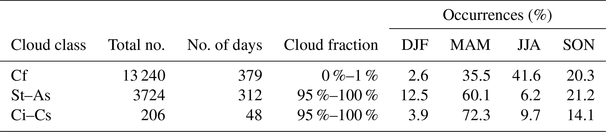
With 13 240 measurements spread over 379 d, the cloud-free data set is the largest. The visual checking of a part of the cloud-free data set allows the conclusion to be drawn that the cloud-free situations are determined with an accuracy of more than 90 %. The same number was also reported in Wacker et al. (2015). The distribution of these measurements per month is slightly different from the one reported in Aebi et al. (2017).

For St–As, in addition to the cloud fraction, further selection criteria are that the direct shortwave radiation does not exceed 1 Wm⁻² (in order to avoid cases of 95 % cloudiness but a clear solar path to the instrument) and that the CBH is equal to or below 5 km. Also, the images of this data set were visually checked and the thick and homogeneous appearance of the cloud layer is confirmed in the remaining data set of 3724 measurements at 312 d.

As reported in Aebi et al. (2018), there are some uncertainties with the automatic detection of thin high-level clouds. Therefore, for the final Ci–Cs data set of 206 measurements, only situations with a measured CBH of at least 5 km are considered. Additionally, the remaining cases were checked visually to avoid misclassifications. This data set is much smaller than the one for St–As clouds due to the fact that the occurrence of overcast Ci–Cs is less frequent in Payerne (Aebi et al., 2017).

3 Methods

In the present study, we use radiative closure in shortwave radiation as a tool to retrieve COT_DSR values. The optical thickness (τ) is defined as the extinction (β_e) of radiation along a path from the surface (z_surf) to the top of atmosphere (z_TOA),

$$\begin{array}{}\text{(1)}& \mathit{\tau }(z_{\mathrm{surf}},z_{\mathrm{TOA}})=\underset{z_{\mathrm{surf}}}{\overset{z_{\mathrm{TOA}}}{\int }}{\mathit{\beta }}_{\mathrm{e}}\left(z\right)\mathrm{d}z,\end{array}$$

where τ is the sum of the optical thickness of the different atmospheric components at a certain wavelength λ,

$$\begin{array}{}\text{(2)}& \begin{array}{rl}\mathit{\tau }\left(\mathit{\lambda }\right)& ={\mathit{\tau }}_{\mathrm{cloud}}\left(\mathit{\lambda }\right)+{\mathit{\tau }}_{\mathrm{AOD}}\left(\mathit{\lambda }\right)+{\mathit{\tau }}_{\mathrm{IWV}}\left(\mathit{\lambda }\right)+{\mathit{\tau }}_{{\mathrm{O}}_{\mathrm{3}}}\left(\mathit{\lambda }\right)\\ & +{\mathit{\tau }}_{\mathrm{Rayleigh}}\left(\mathit{\lambda }\right)+{\mathit{\tau }}_{\mathrm{g}}\left(\mathit{\lambda }\right)\end{array}\end{array}$$

where τ_cloud(λ) is the optical thickness of clouds (in this paper abbreviated as COT), τ_AOD(λ) the optical thickness of aerosols, τ_IWV(λ) the optical thickness of water vapour, ${\mathit{\tau }}_{{\mathrm{O}}_{\mathrm{3}}}\left(\mathit{\lambda }\right)$ the optical thickness of ozone, τ_Rayleigh(λ) the optical thickness due to Rayleigh scattering and τ_g(λ) the optical thickness of other absorbing gases depending on the wavelength.

Assuming spherical droplets in a water cloud, the optical properties COT, SSAc and the asymmetry factor (which is the first moment of the droplet phase function) can be calculated from Mie theory (Stephens, 1978). However, assuming a homogeneous and plane-parallel water cloud layer, the SSAc and the phase function of the cloud droplets play a minor role in the determination of the transmission of the cloud layer, in contrast to COT (Rawlins and Foot, 1990). Under this consideration, the shortwave radiative effect of a water cloud can be either characterised by the COT alone or by a combination of the r_eff and the LWC (Leontyeva and Stamnes, 1994). For the shortwave radiation range, the extinction coefficient in clouds, and thus also COT, has a weak dependence on the wavelength (Slingo and Schrecker, 1982). When r_eff increases, the transmitted flux would decrease because of the larger absorption. However, at the same time, the transmitted flux would also increase because of more forward scattering. The cloud droplet size distribution plays only a minor role in determining the extinction coefficient (Rawlins and Foot, 1990).

Whereas for thick water clouds the transmitted flux only comprises diffuse radiation, the transmitted flux for thin ice clouds comprises direct and diffuse radiation. In this case the Beer–Lambert law could be used to calculate the direct component of the shortwave radiation:

$$\begin{array}{}\text{(3)}& I\left(\mathit{\lambda }\right)=I_{\mathrm{0}}\left(\mathit{\lambda }\right)e^{-m\mathit{\tau }\left(\mathit{\lambda }\right)},\end{array}$$

where λ is the wavelength, I(λ) is the direct transmitted radiation at the surface and I₀(λ) is the irradiance at the top of the atmosphere, m the air mass and τ the sum of the optical thickness as shown in Eq. (2). To determine the cloud optical properties of ice clouds, the microphysical properties particle shape, particle size distribution and ice water content are of interest.

The single scattering albedo (SSA) is defined as the ratio between the scattering and total extinction coefficients and is wavelength dependent. The SSA is the weighted sum of the different components in the atmosphere, namely the single scattering albedo of clouds, of aerosols, of molecules, etc. The SSAc is mainly of importance for the simulation of ice clouds and its values differ depending on the size and shape of the ice crystals (Key et al., 2002). A more complete explanation of the relationships between the optical properties of water and ice clouds is for example given in Kokhanovsky (2004).

3.1 Radiative transfer model and its input parameters

The libRadtran (library of radiative transfer routines and programmes) radiative transfer model version 2.0.2 (Mayer and Kylling, 2005; Emde et al., 2016) is used to simulate the total DSR as well as the direct and diffuse shortwave radiation. Our calculations use the discrete ordinate radiative transfer solver (DISORT) (Stamnes et al., 1988), which solves the one-dimensional plane-parallel radiative transfer equation. The number of streams is six. Increasing the number of streams to the libRadtran maximum of 16 streams would result in a negligible difference in radiation estimations of less than 0.2 % in our calculations. The modelling is performed with the representative wavelength approach (REPTRAN) (Gasteiger et al., 2014) at a coarse resolution (15 cm⁻¹ band width). The calculated spectral range for DSR is 250–3000 nm.

The following atmospheric input parameters are defined for the libRadtran simulations.

Aerosols. For cloud-free cases, the AOD is a daily mean value from the two MODIS instruments at 550 nm. For cloudy conditions, when AOD can not be measured from the ground or from space, or in cases of missing AOD values during cloud-free conditions, the AOD is a monthly mean value from MODIS data over the whole time period analysed. The aerosol profile is assumed to be a standard profile for a rural area described in Shettle (1989) and the aerosol SSA value is assumed to be 0.95.

IWV. For all cases, the IWV is a daily mean (or, if missing, the interpolated mean) value from GPS measurements in Payerne.

Ozone. The total column ozone is the daily mean (or, if missing, the interpolated mean) of measured values of the OMI satellite.

Atmospheric profiles and surface pressure. The surface pressure is a daily mean value from measurements in Payerne. A standard mid-latitude atmospheric profile for either winter or summer is used with standard profiles of pressure, temperature, air density and concentrations of different atmospheric gases (Anderson, 1986). The profiles are scaled to the input values IWV, ozone, surface temperature and pressure. The use of measured profiles of pressure, temperature and relative humidity from radiosondes has a negligible effect on the cloud-free diffuse radiation (0.3 %), and therefore the analyses are performed with the standard profiles.

Albedo. The shortwave surface albedo is calculated from the ratio of the USR to the DSR with 1 min resolution. The mean shortwave surface albedo is 0.24 with a variability of 0.15 and 0.45 (covering 90 % of the data set) in the period analysed. In the few cases of snow the albedo can reach values up to 0.8. Due to the homogeneous landscape around the aerological station of Payerne, the albedo derived from point measurements may be extrapolated to a larger region around the station.

SZA. The SZA is retrieved with a solar position algorithm for every measurement. The analysed data set includes SZA values between 23 and 65^∘.

Water clouds. The low- to mid-level St–As are water clouds simulated with the parametrisation described in Hu and Stamnes (1993). They are assumed to be a plane-parallel and homogeneous cloud layer. The extinction coefficient for shortwave radiation is approximated from a vertical profile of LWC, r_eff and the water density (Slingo and Schrecker, 1982). Assuming a constant LWC of 0.28 g m⁻³ (Hess et al., 1998), r_eff of 10 µm (Stephens, 1994), and a cloud vertical thickness of 2 km and knowing the CBH from the ceilometer measurements result in a large relative mean difference (modelled minus measured divided by measured) and standard deviation of the total DSR of $-\mathrm{54}\mathit{\%}\pm \mathrm{21}\mathit{\%}$, clearly demonstrating that a simulation with these default values does not provide adequate results.

Ice clouds. The high-level Ci–Cs clouds are assumed to be complete ice clouds and are modelled with the parametrisation by Key et al. (2002). The optical property COT of ice clouds is parametrised using a vertical profile of ice water content (IWC) and effective ice crystal radius. The IWC is assumed to be 0.03 g m⁻³ (Korolev et al., 2007; Navas-Guzmán et al., 2014) and the effective ice crystal radius 20 µm (Stubenrauch et al., 2013). The CBH is taken from ceilometer measurements and the cloud vertical thickness is assumed to be 1.5 km, which is a typical value for these high-level clouds (IPCC, 2013). The assumed shape of the ice crystals is a solid column. Using these default values to estimate the total DSR results in a relative mean difference between the modelled and measured total DSR values of $-\mathrm{24}\mathit{\%}\pm \mathrm{8}\mathit{\%}$, also demonstrating that these default values do not produce reliable results.

COT and SSAc. For the simulation of the cloud cases, in addition to the profiles of LWC and r_eff, a COT and/or a SSAc value can also be explicitly defined as input to the model. To iteratively derive COT_DSR, we used COT as an input (see Sect. 3.2). To iteratively derive SSAc for the Ci–Cs cases, we used the estimated COT_DSR as well as SSAc as inputs.

3.2 COT_DSR, SSAc and r_eff retrieval

The aim of our study is to determine COT_DSR (for St–As and Ci–Cs), SSAc (for Ci–Cs) and r_eff (for St–As). In order to retrieve COT_DSR and SSAc, we derive the total DSR as well as its components, direct and diffuse radiation, from libRadtran and compare these simulated values with the corresponding measured DSR data. For St–As, we simulate the DSR (in this case it is composed only of diffuse radiation) with one free RTM input parameter, the COT. The COT input values vary from 1 to 160. The value of COT that minimises the difference between the measured and modelled diffuse DSR is taken as our COT_DSR. Similarly for Ci–Cs, a lookup table is created for two RTM outputs (diffuse and direct radiation), with two free RTM input parameters (COT and SSAc). The COT input values for Ci–Cs vary between 0 and 5. The SSAc input values are between 0.8 and 1. Also here, the COT and SSAc input values that minimise the difference between the measured and modelled direct and diffuse radiation are taken as our COT_DSR and SSAc values, respectively.

In addition, for St–As, we estimate r_eff,

$$\begin{array}{}\text{(4)}& r_{\mathrm{eff}}\approx {\displaystyle \frac{\mathrm{3}\mathrm{LWP}}{\mathrm{2}{\mathit{\rho }}_{\mathrm{lw}}{\mathrm{COT}}_{\mathrm{DSR}}}},\end{array}$$

where LWP is the liquid water path, COT_DSR the cloud optical thickness estimated with the aforementioned method and ρ_lw the density of liquid water (Stephens, 1994).

4 Sensitivity analysis

The aim of the method-related sensitivity analysis is to examine the robustness of the estimated variables COT_DSR and SSAc. In a first step, we examine the uncertainties as well as the sensitivities of the RTM input parameters. For our analysis, we assume that all input variables are independent and uncorrelated, and hence their influence on the radiation output can be estimated by varying each input parameter separately. This assumption is true for a large part of the data set; however, for example, the snow cases with high albedo values have an influence on the sensitivity and thus on the uncertainty of COT_DSR and are thus not completely independent. In a second step, we multiply the standard uncertainties u by the estimated sensitivities, resulting in an uncertainty value u_xxx per parameter. In a third step, we calculate the combined uncertainties u_c and thereafter the expanded combined uncertainties U_c, defining with which uncertainty 95 % of the radiation data can be simulated under the different sky conditions (assuming a normal distribution). These U_c values are thereafter used to estimate the uncertainties of the COT_DSR and SSAc retrieval.

Table 2 Uncertainty analysis for the downward shortwave radiation variables (tot: total, dir: direct, dif: diffuse) under different cloud conditions in absolute (Wm⁻²) and relative (%) numbers (in brackets). Cf: cloud-free, St–As: stratus–altostratus, Ci–Cs: cirrus–cirrostratus, u: standard uncertainty of the variables, u_xxx: u multiplied by the sensitivity value, u_c: combined standard uncertainty, and U_c: expanded combined uncertainty (covering 95 % of the data set). The sensitivities were estimated with assumed COT input values of 38 (for St–As) and 0.8 (for Ci–Cs). Estimated irradiances to calculate the relative numbers: Cf tot: 942 Wm⁻², St–As dif: 156 Wm⁻², Ci–Cs dir: 202 Wm⁻², Ci–Cs dif: 443 Wm⁻².

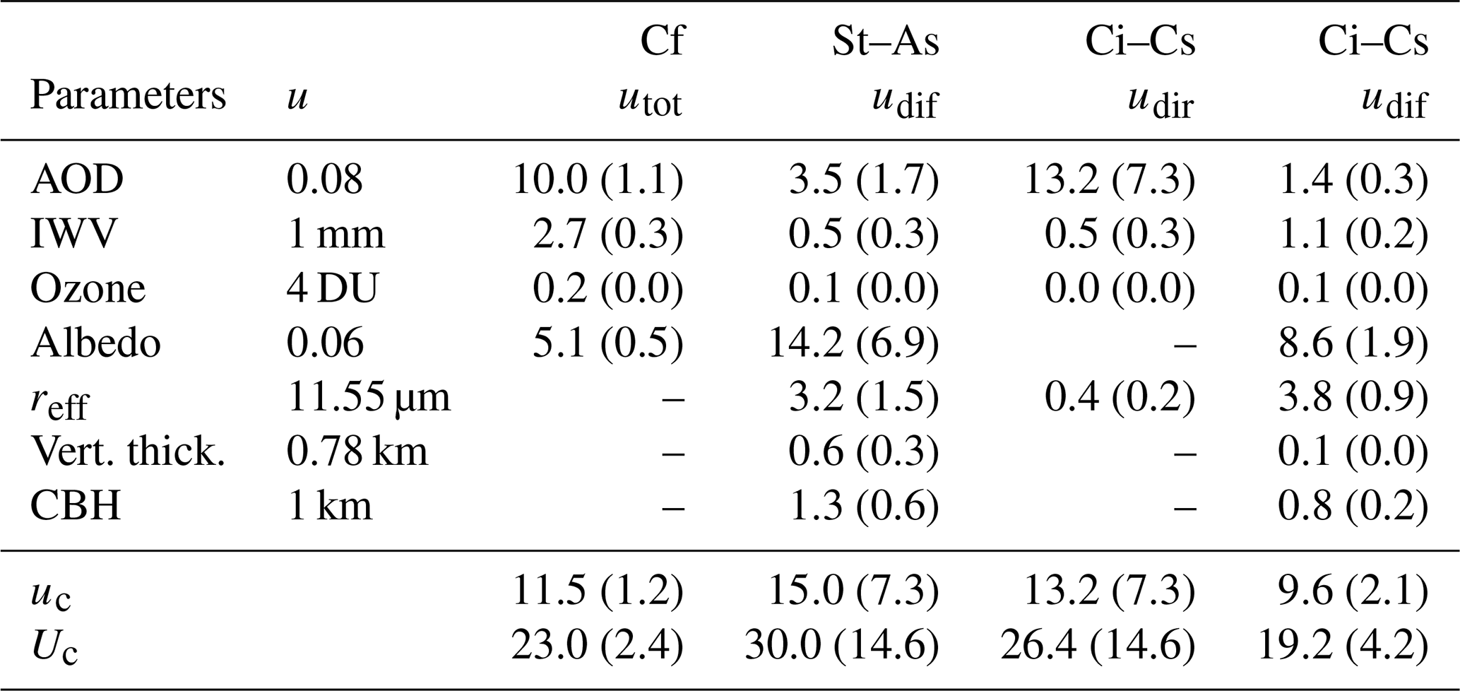
Table 3 Uncertainty analysis for estimated COT_DSR values for stratus–altostratus (St–As) and cirrus–cirrostratus (Ci–Cs) and SSAc for Ci–Cs. Dif: diffuse, Dir: direct radiation, meas: measured, mod: modelled, U: standard uncertainty of the variables, U_xxx: U multiplied by the sensitivity value, and U_c: expanded combined uncertainty. The values were estimated with assumed COT input values of 38 (for St–As) and 0.8 (for Ci–Cs).

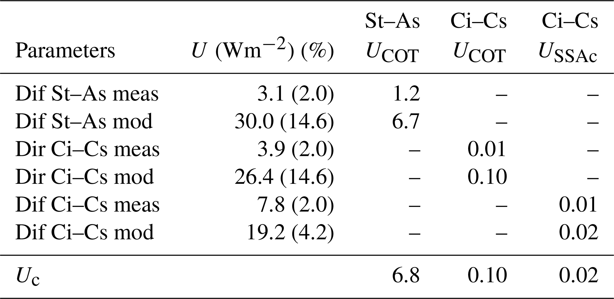
The assumed uncertainties are Type B uncertainties, which are uncertainties that are not based on statistical analysis, but rather on uncertainties specified in the literature, experience or previous measurements (Guide to the Expression of Uncertainty in Measurement (GUM); BIPM, 2008). The uncertainties for the cloudy cases presented in Tables 2 and 3 are estimated for the example cases for which COT input values are equal to 38 and 0.8 for St–As and Ci–Cs, respectively. The expanded combined uncertainties for COT_DSR values were additionally estimated for other COT input values between 10 and 100 (St–As) and 0 and 5 (Ci–Cs), but are not presented here. In summary, for St–As, the larger the estimated COT_DSR value, the larger the absolute expanded combined uncertainty value U_c. However, in relative uncertainties, independent of the estimated COT_DSR value, the uncertainty is around 18 %. For Ci–Cs the opposite applies: the absolute U_c in COT_DSR retrieval is 0.1 for all cases, independent of the COT input value. Similar behaviours of the uncertainties of COT_DSR estimations are also presented in Serrano et al. (2014).

The estimated standard uncertainties u for the specified input parameters in the libRadtran model are shown in Table 2 (second column). The standard uncertainty for IWV is taken from the literature (Morland et al., 2006b).

The AOD data set consists of daily and monthly mean values, respectively. Therefore, the uncertainty u for the AOD values under cloud-free conditions is estimated from the standard deviation comparing the used MODIS L3 C6 AOD values with the measured PFR AOD data, where the mean difference is zero with a standard uncertainty of 0.07. For cloudy conditions, AOD can be measured by neither the PFRs nor by satellites. Assuming a rectangular distribution of the data, the uncertainty u is calculated by dividing the half width of 95 % of the data set (a) by the root of 3 ($u=\frac{a}{\sqrt{\mathrm{3}}}$). For AOD, under cloudy conditions, u was estimated with this formula for different seasons separately. The resulting uncertainty is 0.08, which is the standard uncertainty value used for AOD.

The uncertainty u for albedo was calculated with the same equation, also taking into account 95 % of the data set, assuming a rectangular distribution and for different seasons separately, but neglecting the occasional snow events. The resulting u value for albedo is 0.06.

The uncertainty of total column ozone is assumed to be 1 % (Levelt et al., 2018), which corresponds to an uncertainty of about 4 DU.

The effective droplet and ice crystal radius values are assumed to be between 5 and 45 µm, also with a rectangular distribution and thus resulting in u=11.55 µm.

The sensitivities of the input parameters under cloudy conditions in Table 2 were calculated with cloud optical thickness values defined in the libRadtran input file. Consequently, in the analysed cases, the LWC has a negligible influence on the calculation of the COT_DSR and is therefore not listed in Table 2. Also not listed are all variables that were not specifically defined in our analysis due to lack of available measurement data.

The total DSR under cloud-free conditions can be simulated with an expanded combined uncertainty of 2.4 %. Thus, this uncertainty is in a similar range to the instrument-related shortwave radiation measurement uncertainty. Almost half of the estimated expanded combined uncertainty is caused by the uncertainty of the AOD (1.1 %) (Table 2, third column). The contribution to the uncertainty of the input parameters IWV and total column ozone is negligible.

For the simulation of the diffuse DSR under a St–As cloud with a COT_DSR value of 38, the parameter contributing most to the standard uncertainty of 7.3 % is the albedo with 6.9 %. The second largest contributor to the uncertainty budget is AOD with 1.7 % and hence represents a variable which in practice can not be measured in the presence of a stratus cloud. The influence of the macrophysical properties, both cloud vertical thickness and CBH, on the DSR is negligible. The expanded combined model uncertainty (14.6 %) of the diffuse DSR under a stratus–altostratus cloud is thereafter used to estimate the uncertainty of the retrieved COT_DSR values shown in Table 3.

For the simulation of the direct radiation under a cirrus–cirrostratus cloud with COT_DSR equal to 0.8, the expanded combined uncertainty is, at 14.6 %, much larger than the model uncertainty of the diffuse radiation (4.2 %) under the same cloud conditions. Whereas for the direct radiation the dominant contributor to the expanded uncertainty is AOD (7.3 %), the main contributor to the expanded uncertainty of the diffuse radiation is the albedo (1.9 %).

The estimated model uncertainties presented in Table 2 are then used to calculate the expanded combined uncertainties of the COT_DSR retrieval (summarised in Table 3). The retrieval method of the COT_DSR values for St–As conditions presented here has a U_c of 6.8. The expanded combined uncertainties under Ci–Cs are for COT_DSR and SSAc 0.10 and 0.02, respectively.

5 Results

The optical thickness τ in the radiative transfer equation is a sum of optical thickness values of different atmospheric components (see Eq. 2). Therefore, to determine the optical thickness of clouds, the model is first validated for cloud-free values (τ_clouds=0) by assuring that including all other input parameters in the model leads to a reasonable calculation of the downward shortwave radiation.

5.1 Cloud-free

In the period 1 January 2013 to 31 December 2017, 13 240 cloud-free measurements on 379 d with SZA below 65^∘ are available. The simulations of the total DSR for cloud-free cases show a very good agreement in comparison to the measurements. The absolute and relative (absolute difference divided by the measured value) mean differences between the modelled and measured total DSR are 6 ${\mathrm{Wm}}^{-\mathrm{2}}\pm \mathrm{12}{\mathrm{Wm}}^{-\mathrm{2}}$ and 0.9 %±2.1 %, respectively. Thus the model slightly overestimates the total DSR measurement, but the agreement is within the measurement uncertainty of the instrument (2 %) (Vuilleumier et al., 2014) as well as within the estimated expanded combined uncertainty of 2.4 % (discussed in Sect. 4). The good agreement between the modelled and measured total DSR is also demonstrated in the high correlation coefficient (r=0.996). There is no temporal trend in the difference between the modelled and measured total DSR throughout the whole time period, which confirms the stability of the instrument as already discussed in Vuilleumier et al. (2014). Analysis of the difference between the simulated and measured total DSR values per day of year shows no seasonal dependence of the agreement. Consequently, we can conclude that the simulation of the total DSR under cloud-free conditions is excellent.

Comparing separately the two components of the total DSR (direct and diffuse) shows that, in general, the direct radiation has a larger correlation (r=0.98) between measurements and simulations than the diffuse component (r=0.73). The better agreement of the direct radiation is also reflected in the relative mean difference (modelled minus measured divided by measured) of $-\mathrm{0.2}\mathit{\%}\pm \mathrm{6.2}\mathit{\%}$ in comparison to the relative mean difference of the diffuse radiation of 10.0 %±21.5 %.

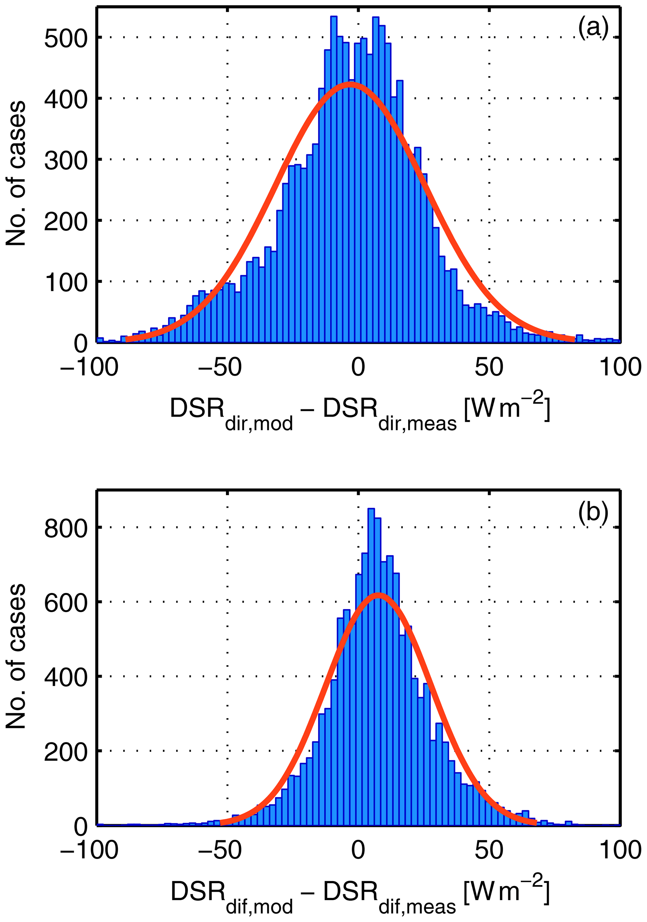
Figure 2 Distribution of the differences between modelled and measured downward shortwave radiation (DSR) for cloud-free cases for the (a) direct and (b) diffuse components.

Figure 2 shows the distribution of the absolute differences between the modelled and measured direct (top) and diffuse (bottom) radiation. On average, the model slightly underestimates the measured direct radiation by −3 ${\mathrm{Wm}}^{-\mathrm{2}}\pm \mathrm{29}$ Wm⁻² and the modelled diffuse radiation slightly overestimates the measurement by 8 ${\mathrm{Wm}}^{-\mathrm{2}}\pm \mathrm{20}$ Wm⁻². The small difference between the modelled and measured direct radiation can for example be explained by uncertainties due to differences in the forward scattering due to different fields-of-view of the instrument and the model (Blanc et al., 2014) or by differences in the actual and RTM-used extraterrestrial solar irradiance. However, the good agreement in the direct radiation confirms the proper use of the RTM AOD inputs under cloud-free conditions. Part of the larger difference in the diffuse radiation can be explained by the use of default values for the atmospheric profiles instead of radiosonde data. However, as discussed in Sect. 3.1, this difference is small. Adjusting the aerosol SSA in each case also decreases the difference in the diffuse radiation. However, due to the lack of aerosol SSA measurements, no further improvement in such deviations is possible in the current study. In summary, we found a similar agreement in the total and direct shortwave radiation as other groups in the past (e.g. Kato et al., 1997; Michalsky et al., 2006; Nowak et al., 2008a; Wang et al., 2009; Ruiz-Arias et al., 2013; Dolinar et al., 2016).

Consequently, because the simulation of DSR under cloud-free conditions achieved an agreement with the measured DSR within measurement and model uncertainty, we assume that all input parameters in Eq. (2), except the COT, are well-defined. Subsequently, a similar model layout is used to simulate the DSR under cloudy conditions.

5.2 COT_DSR, SSAc and r_eff estimations

5.2.1 Stratus–altostratus

The data set of St–As consists of 3724 measurements collected on 312 d. In cases of thick, low-level water clouds, the direct component of the radiation is less than 1 Wm⁻². Thus, for these cases the total DSR is nearly only diffuse radiation due to multiple scattering in and around the cloud. In the case of low-level clouds, the most relevant optical property for the simulation of cloudy conditions is the COT. The default SSAc value used for the simulation of radiation can be a source of uncertainty in the COT_DSR determination. Nevertheless, Rawlins and Foot (1990) pointed out that it is an input parameter of minor importance for this cloud class.

The resulting distribution of the estimated COT_DSR values for our data set in Payerne is shown in Fig. 3. The arithmetic mean COT_DSR value and standard deviation retrieved from our analysis is 39±21. Considering a lognormal distribution, the geometric mean of 33.8 with a geometric standard deviation of 1.7 represents a range in COT_DSR values between 20 and 56. The variability of COT_DSR values is much larger than the expanded combined uncertainty U_c of the COT_DSR retrieval. Thus, the large variability in COT_DSR values for St–As cases in Payerne reflects the inhomogeneity of these clouds and is not due to the uncertainty in the retrieval method. Ninety-five percent of the COT_DSR values for the St–As data set are between 12 and 92. This finding of a minimum COT_DSR value of 12 agrees with the findings of Bohren et al. (1995) stating that the direct shortwave radiation is blocked if COT is larger than 10.

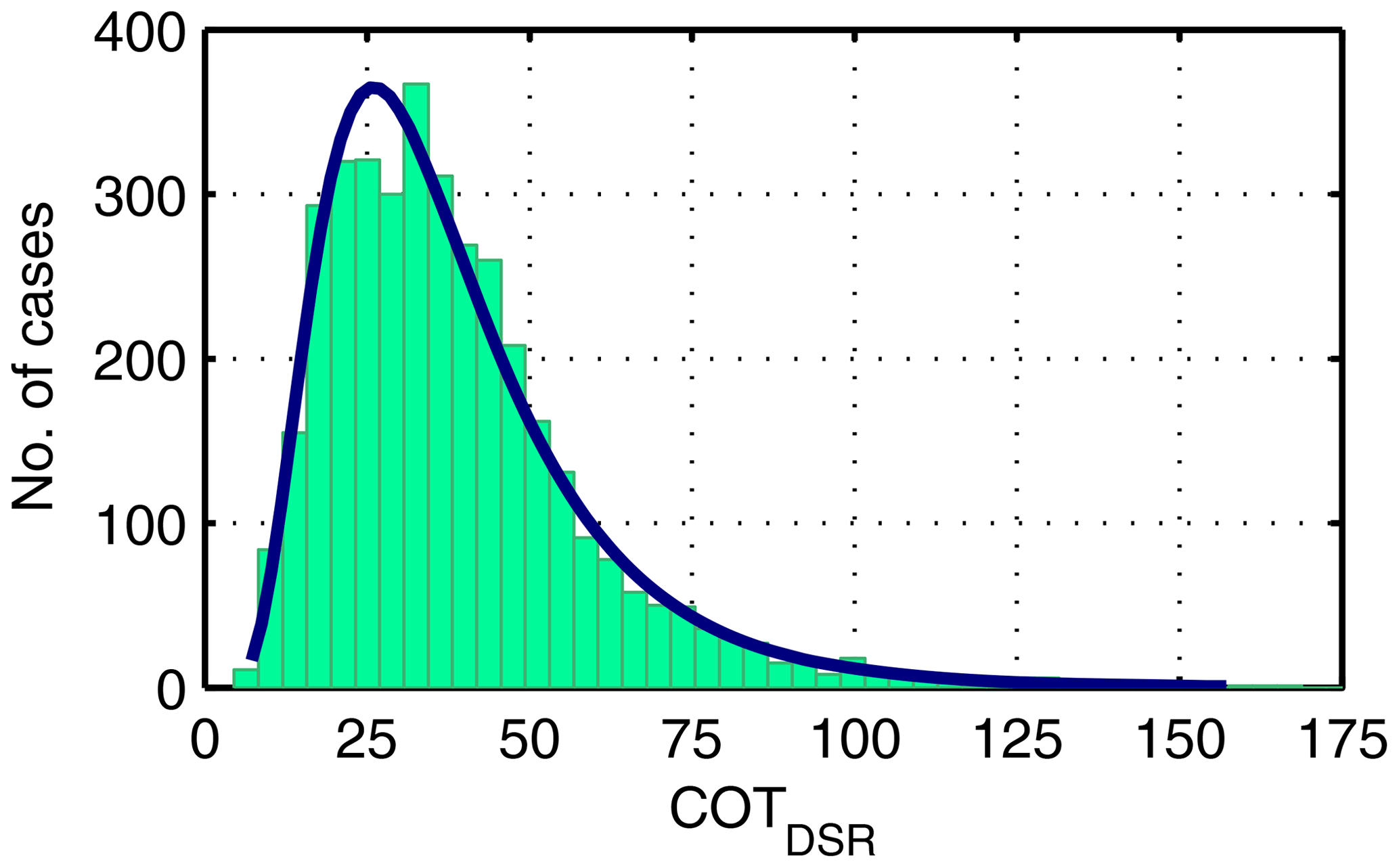
Figure 3 Distribution of COT retrieved from DSR (COT_DSR) for stratus–altostratus cases in Payerne. The geometric mean COT_DSR value is 33.8 with a geometric standard deviation of 1.7.

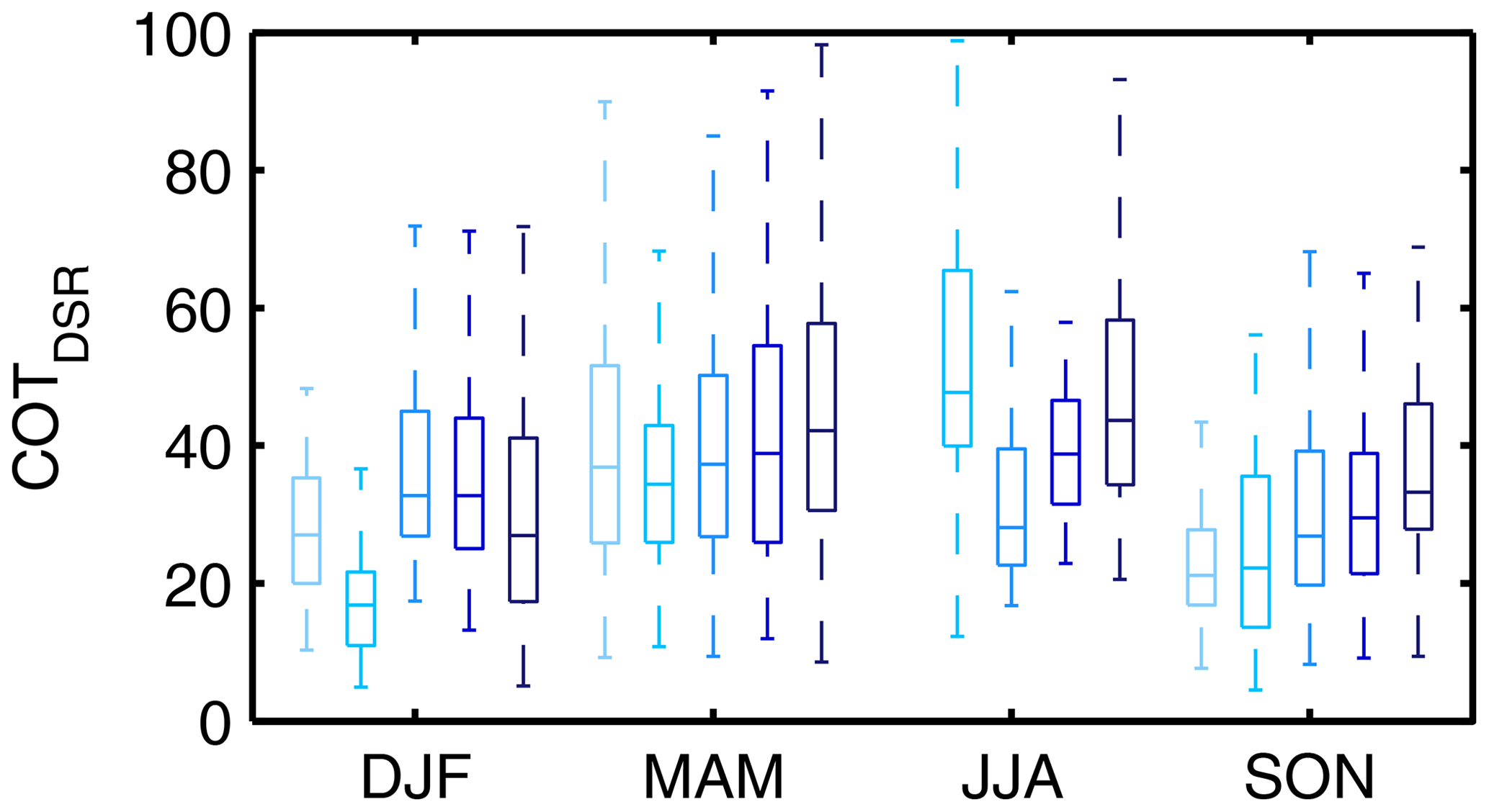
Figure 4 Distribution of the COT_DSR values per season (DJF: winter, MAM: spring, JJA: summer, SON: autumn) and years (light to dark blue: 2013 to 2017) of St–As in Payerne. The boxplots show the median, the interquartile range and the 95 % intervals of the COT_DSR values. No data in JJA 2013.

Figure 4 shows the distribution of the COT_DSR values in different seasons and years. The boxplots show the median, the interquartile range and the 95 % intervals of the COT_DSR values. It demonstrates that the COT_DSR values are in general higher in spring (MAM) and summer (JJA) than in autumn (SON) and winter (DJF). This finding is consistent with a study presenting the COT distribution over the seasons at different stations in China (Li et al., 2019). Also Lindfors and Vuilleumier (2005) found higher COT values in summer than in winter at two different stations (Davos and Sodankylä). One potential explanation is discussed in Barker et al. (1998) that in winter the air is colder and thus also drier, which leads to optically thinner clouds. In our St–As data set it seems that in spring and autumn the COT_DSR values increase with time. But our data set is too small to draw any conclusions about a trend. Nevertheless, Barker et al. (1998) also presented a weak increasing trend in COT values at different stations in Canada over a 30-year period.

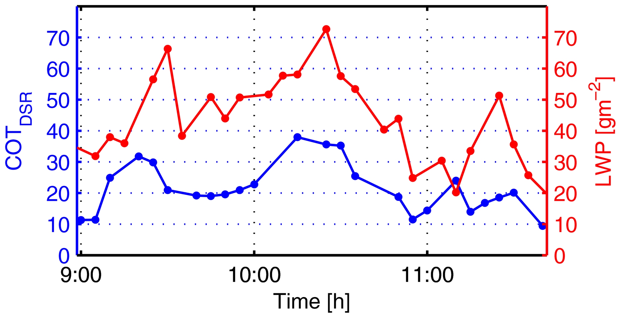
Figure 5 Time series of the COT_DSR (blue) and LWP (red) during St–As conditions in Payerne on 15 March 2015 from 09:00 to 11:45 UTC.

Figure 5 shows the fluctuation of COT_DSR (blue) and LWP (red) within a few hours on 15 March 2015 during St–As conditions. Within a short time period (less than 40 min), the COT_DSR decreases about 20–30 units (in Fig. 5 between around 10:15 and 10:45 UTC). The visual checking of the corresponding images confirms nicely the dissipation of the thick cloud layer to a thinner one. This dissolving of the cloud layer in Payerne around local noon also matches the typical meteorological situation of the location. The change in COT_DSR also correlates with independent measurements of LWP from a HATPRO instrument: the smaller the COT_DSR, the smaller the LWP value. The short-term changes in COT_DSR values (two consecutive measurements 5 min apart) of less than 5 are within the COT_DSR retrieval uncertainty, which is discussed in Sect. 4.

The COT_DSR values of St–As are thereafter used to estimate r_eff using Eq. (4). For this estimation all LWP data with values greater than 400 g m⁻² are neglected due to the presence of rain as well as all values below 30 g m⁻² because this threshold corresponds to cloud-free conditions (Löhnert and Crewell, 2003). The determined mean r_eff for our St–As data set is 7 µm ±5 µm. The mean value agrees with the value presented in Hess et al. (1998) for continental stratus clouds. The 2.5th and 97.5th percentiles of the determined r_eff are 2 and 20 µm, respectively.

5.2.2 Cirrus–cirrostratus

A similar analysis to the one for St–As is also performed for the high-level cloud class Ci–Cs. As already mentioned in Sect. 2.2, the data set of Ci–Cs consists of 206 measurements on 48 d. The distribution of the COT_DSR values estimated from the direct shortwave irradiance is shown in Fig. 6.

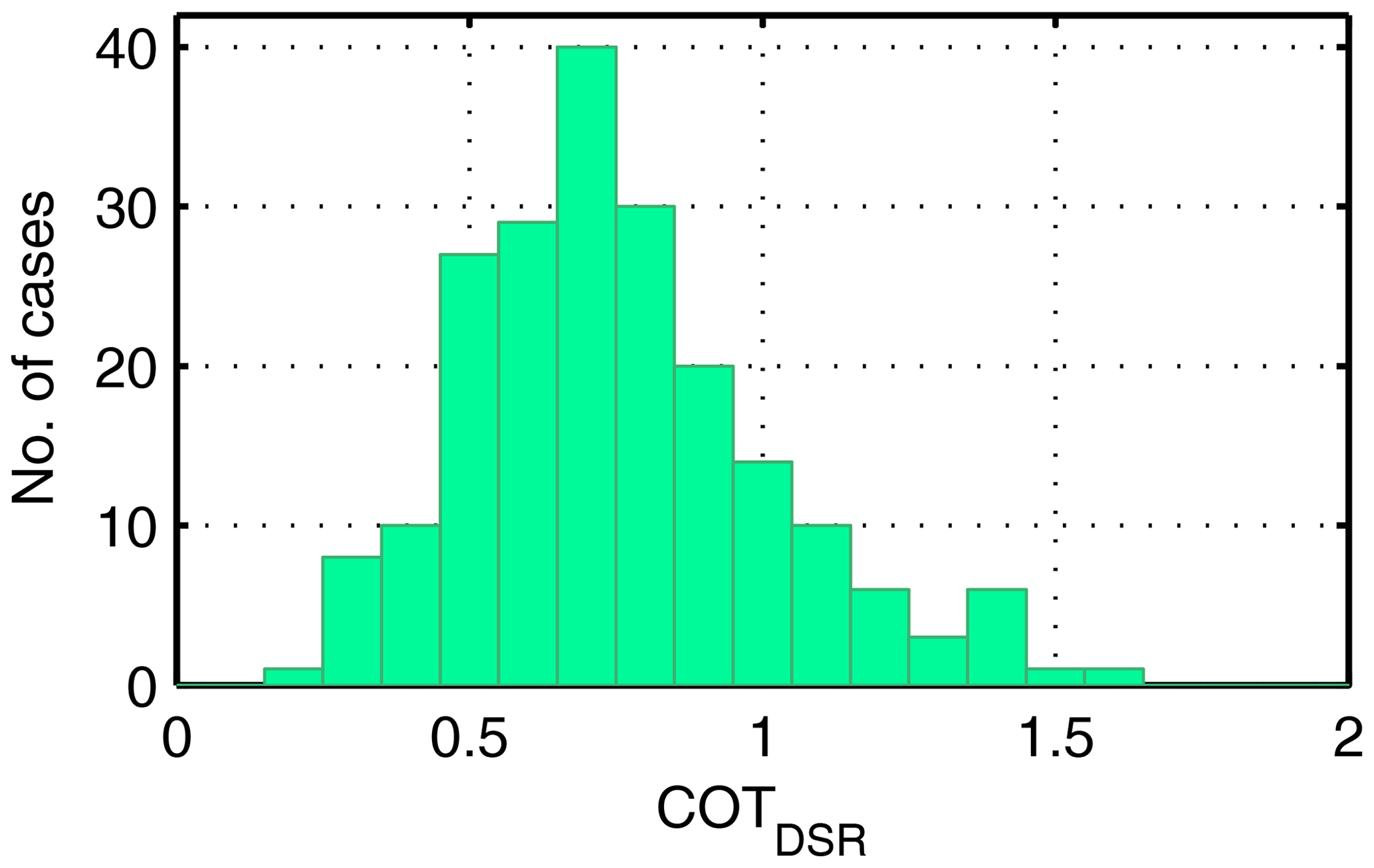
Figure 6 Distribution of COT_DSR retrieved from direct DSR for cirrus–cirrostratus cases in Payerne. The mean COT_DSR value is 0.75±0.26.

The mean COT_DSR is 0.75±0.26 and 95 % of the COT_DSR values vary between 0.32 and 1.40 and are thus in a similar range to that, for example, presented in Giannakaki et al. (2007) and Hong and Liu (2015). Also, the expanded combined uncertainty of the COT_DSR retrieval method under Ci–Cs conditions (0.10) is much smaller than the 1-sigma COT_DSR variability (0.26). The latter therefore also reflects the large variability in the COT_DSR values in the Ci–Cs data set.

The COT_DSR values retrieved are used as input to libRadtran in order to estimate the SSAc values for Ci–Cs. The mean SSAc value and its standard deviation retrieved are 0.92±0.04 (Fig. 7) and therefore slightly larger than the libRadtran default value of 0.87 (Key et al., 2002).

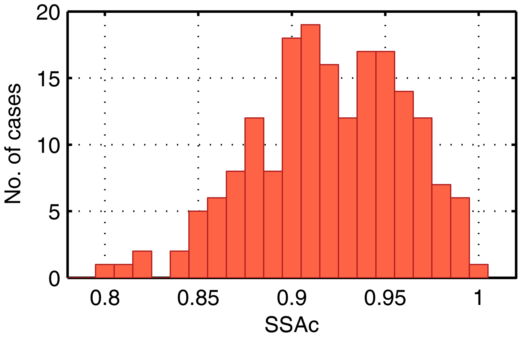
Figure 7 Distribution of SSAc retrieved from diffuse DSR for cirrus–cirrostratus cases in Payerne. The mean SSAc value is 0.92±0.04.

Ninety-five percent of the SSAc data are between 0.84 and 0.99. Therefore, we can conclude that the SSAc values defined by Key et al. (2002) mostly underestimate the extinction by scattering for the cirrus–cirrostratus data set in Payerne.

The SSAc under Ci–Cs conditions can be determined with an uncertainty of 0.02, which is smaller than the 1-sigma variability of 0.04. Thus, the variability in the results for SSAc is larger than the model uncertainty and confirms the importance of accurate knowledge of the SSAc values for high-level clouds.

6 Comparison of COT_DSR with independent data sets

6.1 Barnard and Long equation

Our retrieved COT_DSR values for St–As are compared to COT values estimated by applying the empirical equation by Barnard and Long (2004),

$$\begin{array}{}\text{(5)}& {\mathit{\tau }}_{\mathrm{c}}=\exp \left[\mathrm{2.15}+A+\mathrm{1.91}\times \mathrm{arctanh}\left(\mathrm{1}-\mathrm{1.74}\times {\displaystyle \frac{D}{C{\mathit{\mu }}_{\mathrm{0}}^{\frac{\mathrm{1}}{\mathrm{4}}}}}\right)\right],\end{array}$$

where τ_c is the cloud optical thickness (here COT_Barnard), A is the surface albedo, D the measured broadband diffuse radiation, C a radiation value from a clear-sky model and μ₀ the air mass. In the current study the clear-sky model values are estimated according to Aebi et al. (2017).

The correlation between the COT_DSR and COT_Barnard is very high (r=0.99) (Fig. 8). The mean COT difference between these two retrieval methods is $-\mathrm{1.2}\pm \mathrm{2.7}$, showing a slight underestimation of COT_Barnard. However, this difference is within the model uncertainty.

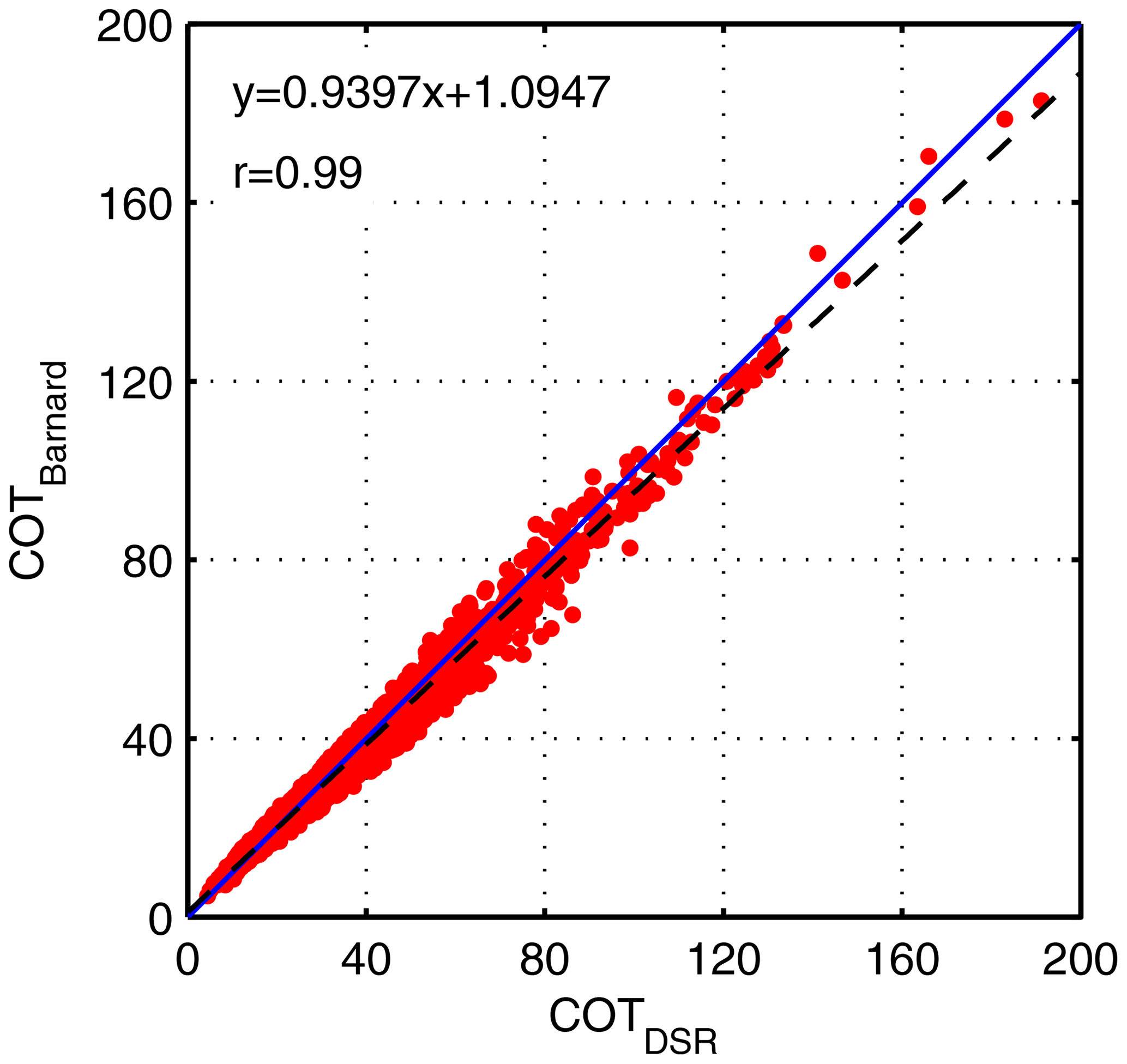
Figure 8 Correlation between COT values retrieved from DSR (COT_DSR) and from the equation presented in Barnard and Long (2004) (COT_Barnard) for St–As in Payerne.

The COT estimation formula presented in Barnard and Long (2004) is only valid for thick clouds with COT values larger than 10. Consequently, this formula can not be applied to Ci–Cs cases because the diffuse radiation is not the correct component for estimation of the COT.

6.2 MODIS

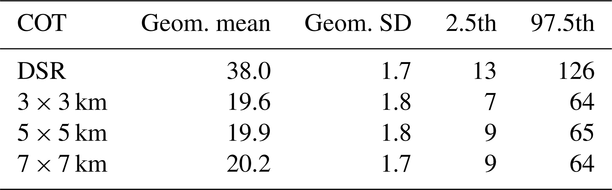
The COT_DSR values are also compared with L2 C6.1 COT values from MODIS Aqua (COT_MODIS). The comparison is performed for a subset of the St–As data set, taking into account the overpass time of the MODIS satellite. The analysis is done for MODIS grid cells of 3×3, 5×5 and 7×7 km including Payerne. Considering the mean COT_DSR value from data ± 30 min around the overpass times of the satellite and the highest spatial resolution results in a matching in 169 cases. At 37.6 (geometric standard deviation 1.7), the geometric mean of COT_DSR for this subset is much higher than the geometric mean and standard deviation of COT_MODIS (17.4 and 1.9, respectively).

Considering only the COT_DSR values which have an exact time-match with the COT_MODIS measurements decreases the subset to 60 measurements but does not decrease the difference between COT_DSR and COT_MODIS. The geometric mean, geometric standard deviation and 2.5th and 97.5th percentiles for COT_DSR and COT_MODIS with the different satellite resolutions are shown in Table 4. The COT_DSR is higher than the value mentioned in Sect. 5.2.1 because here only a subset of 60 measurements is taken into account. It is noteworthy that the difference in the mean of COT_MODIS with different resolutions is small. However, at around 18, the difference in the geometric mean between COT_DSR and COT_MODIS is rather high. The correlation between COT_DSR and COT_MODIS for the 3×3 km resolution is r=0.74 (Fig. 9).

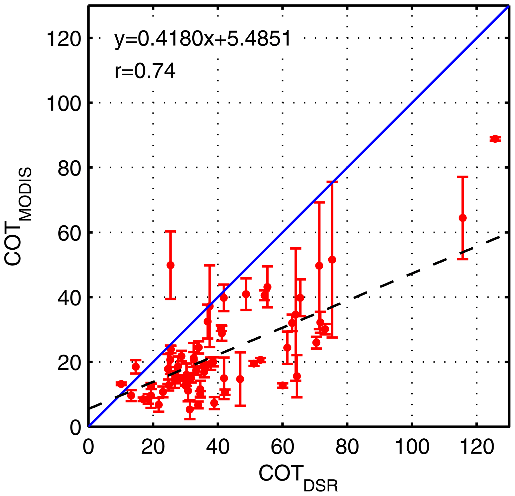
Figure 9 Correlation between COT values retrieved from DSR (COT_DSR) and from MODIS L2 C6.1 data (COT_MODIS), with error bars showing the standard deviation, in a grid cell of 3 × 3 km for St–As including Payerne.

Li et al. (2019) found similar correlation coefficients for stations in China for instantaneous matching of COT data from MODIS and radiometers. In their study the COT_MODIS values are in general also lower than the ground-based COT values. The satellite analysis may only take into account the highest cloud layer, while the values derived from DSR take into account all layers, even though the camera did not allow identification of multiple cloud layers. Another explanation might be the slight difference in the wavelength considered (Baum et al., 2014). Other potential explanations of differences between surface- and satellite-based estimations of COT values are presented in Barker et al. (1998). The same study also shows larger COT values from surface-based data than from satellite-based data.

We also used the COT_MODIS and r_{eff, MODIS} (also L2) and a grid of 3×3 km to calculate the DSR_MODIS with libRadtran. This analysis results in a mean overestimation of the total DSR_MODIS of 88 Wm⁻² in comparison to the measured total DSR during St–As conditions in Payerne.

Other studies (e.g. Painemal and Zuidema, 2011; McHardy et al., 2018) show a better agreement between ground- and satellite-based COT values, but mainly for averaged data over a longer time period (for example monthly means). Our sample of 60 data points is too small to calculate a monthly mean COT_DSR.

Table 4 Geometric mean, geometric standard deviation and 2.5th and 97.5th percentiles of COT retrieved from ground-based broadband shortwave radiation (DSR) and from MODIS L2 data with different spatial resolutions (3×3, 5×5 and 7×7 km) for St–As above Payerne.

Comparing the COT_DSR and COT_MODIS values for Ci–Cs shows only three time-matches. For these three situations, the COT_MODIS is larger than COT_DSR. But the data set is too small to draw any conclusions from this comparison.

6.3 PFR

The COT_DSR values derived for the cirrus–cirrostratus cases are compared with the cloud optical thickness values derived from measurements of direct solar irradiance obtained from four collocated PFR sunphotometers measuring at 16 wavelengths between 305 and 1024 nm (COT_PFR). The COT_PFR values are retrieved at the different channels of the instruments and corrected by the corresponding AOD values for the corresponding day. It is difficult to estimate the effective wavelength that corresponds to the COT_DSR values derived from broadband measurements.

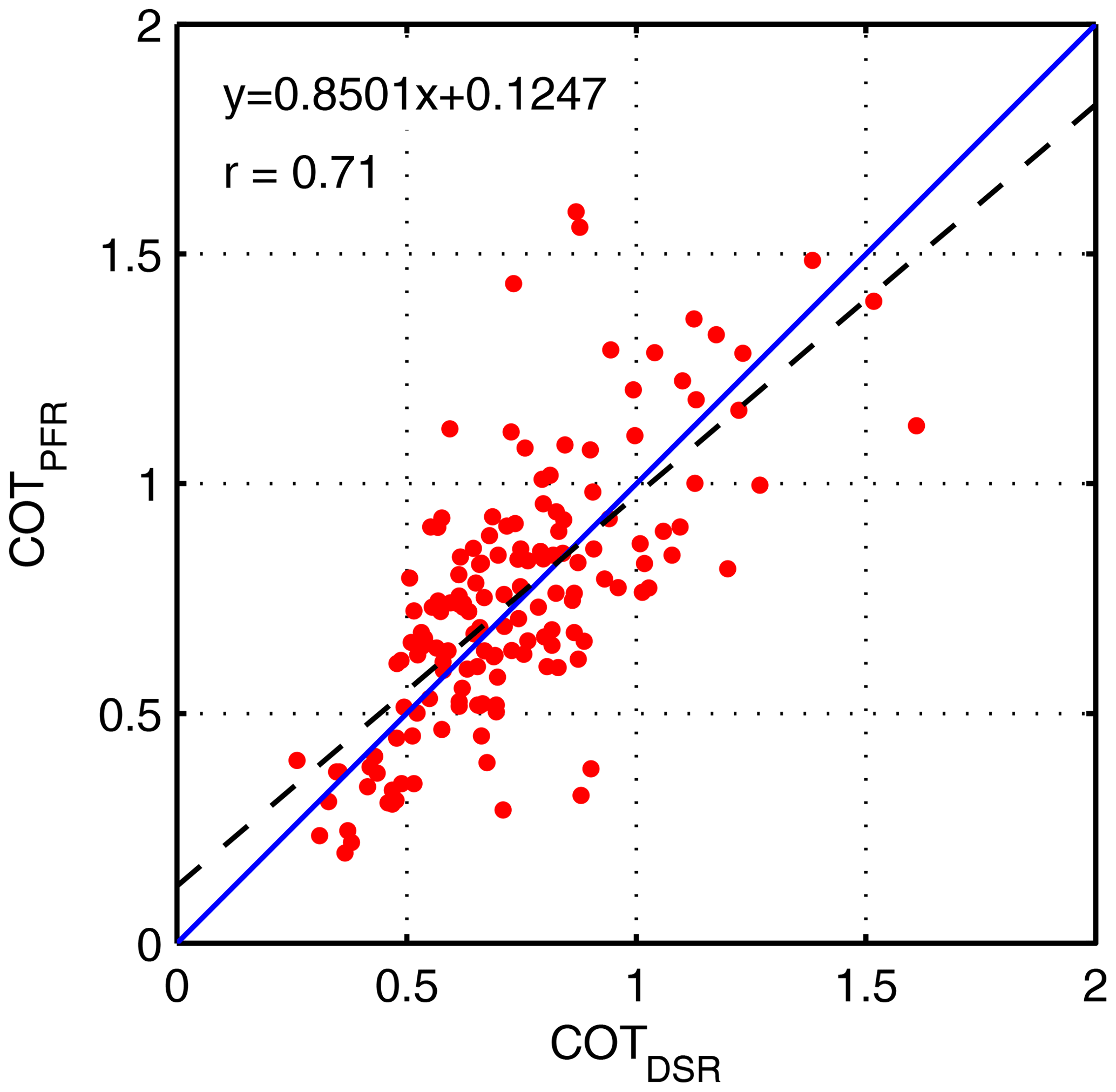
Figure 10 Correlation between COT values retrieved from DSR (COT_DSR) and COT values retrieved from PFR measurements at λ=412 nm (COT_PFR) for Ci–Cs in Payerne.

As an example, Fig. 10 shows a scatter plot of the COT_PFR derived at 412 nm versus COT_DSR. The correlation of the COT between these two independent methods is r=0.71. The slightly higher values of COT_PFR relative to COT_DSR might result from the different spectral regions used to retrieve the cloud optical thickness: the 412 nm channel for the PFR and the complete shortwave spectrum for COT_DSR. The correlation between COT_DSR and COT_PFR at 500 nm is slightly lower (r=0.60). A slight dependence of the wavelength on the retrieved COT values is also confirmed by the analysis of the COT_PFR values retrieved at other wavelengths of the PFRs. Another explanation for the discrepancy might be the enhanced forward scattering entering the field-of-view of the instrument, which causes an overestimation of the measured direct shortwave radiation compared to the modelled one (Blanc et al., 2014). This fact results in an underestimation of COT_DSR of Ci–Cs clouds.

7 Summary and conclusions

The current study presents a method to retrieve COT_DSR, SSAc and r_eff values for the two cloud types stratus–altostratus and cirrus–cirrostratus by combining broadband solar shortwave radiation (total as well as the direct and diffuse components) measurements and simulations with a radiative transfer model. The study is performed with radiation data from the BSRN station, Payerne, Switzerland, which can be seen as a reference station for radiation measurements, and thus our method can also be applied at other stations. In total, more than 3000 St–As measurements and 206 Ci–Cs measurements collocated in the time period 1 January 2013 to 31 December 2017 and in situations with a SZA lower than 65^∘ are analysed.

In order to test the model–measurement combination performance, in a first step more than 13 000 cloud-free measurements were analysed. With a relative mean difference of 0.9 %±2.1 %, the simulated cloud-free total DSR is in agreement with the measured total DSR within instrument uncertainty. The sensitivity analysis shows an expanded model uncertainty (covering 95 % of the data set) of DSR retrieval of less than 2.5 %, and thus the difference is also within the model uncertainty.

Ninety-five percent of the estimated St–As COT_DSR values are between 12 and 92 with a geometric mean and geometric standard deviation of 33.8 and 1.7. The COT_DSR values are higher in spring and summer than in autumn and winter. These estimated COT_DSR values are in very good agreement with the COT_Barnard values estimated using the empirical equation of Barnard and Long (2004). At $-\mathrm{1.2}\pm \mathrm{2.7}$, the mean difference in the COT values between these two methods is within model uncertainty. However, for a subset of the St–As data set, COT_MODIS with a resolution of 3×3 km clearly underestimates our determined COT_DSR values. Using COT_MODIS and r_eff from MODIS to estimate DSR results in a mean overestimation of the total shortwave irradiance of more than 50 % of the measured DSR values under St–As conditions in Payerne. Changing the spatial resolution and/or the matching in time does not result in a smaller difference in the mean COT. These large discrepancies can not be explained at present, but were also shown in other studies (e.g. Li et al., 2019). Therefore, we conclude that for a specific location (in this case Payerne) and for high temporal resolution data, COT_MODIS is not reliable.

The 2.5th and 97.5th percentiles of r_eff under St–As conditions in Payerne are 2 and 20 µm, respectively, and thus are comparable to values presented in other studies (e.g. Hess et al., 1998).

The retrieved mean COT_DSR value under Ci–Cs conditions in Payerne is 0.75±0.26 and thus in a similar range to that described in other studies (e.g. Qiu, 2006; Giannakaki et al., 2007; Hong and Liu, 2015). The comparison of the COT_DSR and COT_PFR values retrieved from PFRs shows correlation coefficients at r=0.60 (500 nm) and r=0.71 (412 nm). The retrieved mean cloud single scattering albedo value for Ci–Cs is 0.92±0.04.

It has been demonstrated that with the herein presented method COT_DSR, SSAc and r_eff can be estimated from state-of-the-art data sets in Payerne and for different cloud conditions. The same method could also be applied at other BSRN stations in order to validate the method. In the case of similar results in the COT_DSR estimation, a long-term data set in cloud properties could be produced and could be of use to increase the availability of cloud optical properties for e.g. climate models.

An extension of this study would be to perform a radiative closure study for longwave radiation for a similar data set. This analysis would be an extension of the study presented by Wacker et al. (2011) which describes a longwave closure study for well-defined stratus nebulosus cases in Payerne. This future analysis is important in order to analyse the effect of cloud microphysical and optical properties on longwave radiation as well and to develop thereafter a more complete picture of the influence of cloud parameters on the surface radiation budget.