Intercomparison of MAX-DOAS vertical profile retrieval algorithms: studies on field data from the CINDI-2 campaign

The second Cabauw Intercomparison of Nitrogen Dioxide measuring Instruments (CINDI-2) took place in Cabauw (the Netherlands) in September 2016 with the aim of assessing the consistency of multi-axis differential optical absorption spectroscopy (MAX-DOAS) measurements of tropospheric species (NO₂, HCHO, O₃, HONO, CHOCHO and O₄). This was achieved through the coordinated operation of 36 spectrometers operated by 24 groups from all over the world, together with a wide range of supporting reference observations (in situ analysers, balloon sondes, lidars, long-path DOAS, direct-sun DOAS, Sun photometer and meteorological instruments).

In the presented study, the retrieved CINDI-2 MAX-DOAS trace gas (NO₂, HCHO) and aerosol vertical profiles of 15 participating groups using different inversion algorithms are compared and validated against the colocated supporting observations, with the focus on aerosol optical thicknesses (AOTs), trace gas vertical column densities (VCDs) and trace gas surface concentrations. The algorithms are based on three different techniques: six use the optimal estimation method, two use a parameterized approach and one algorithm relies on simplified radiative transport assumptions and analytical calculations. To assess the agreement among the inversion algorithms independent of inconsistencies in the trace gas slant column density acquisition, participants applied their inversion to a common set of slant columns. Further, important settings like the retrieval grid, profiles of O₃, temperature and pressure as well as aerosol optical properties and a priori assumptions (for optimal estimation algorithms) have been prescribed to reduce possible sources of discrepancies.

The profiling results were found to be in good qualitative agreement: most participants obtained the same features in the retrieved vertical trace gas and aerosol distributions; however, these are sometimes at different altitudes and of different magnitudes. Under clear-sky conditions, the root-mean-square differences (RMSDs) among the results of individual participants are in the range of 0.01–0.1 for AOTs, (1.5–15) $\times {\mathrm{10}}^{\mathrm{14}}\mathrm{molec}.{\mathrm{cm}}^{-\mathrm{2}}$ for trace gas (NO₂, HCHO) VCDs and (0.3–$\mathrm{8})\times {\mathrm{10}}^{\mathrm{10}}\mathrm{molec}.{\mathrm{cm}}^{-\mathrm{3}}$ for trace gas surface concentrations. These values compare to approximate average optical thicknesses of 0.3, trace gas vertical columns of $\mathrm{90}\times {\mathrm{10}}^{\mathrm{14}}\mathrm{molec}.{\mathrm{cm}}^{-\mathrm{2}}$ and trace gas surface concentrations of $\mathrm{11}\times {\mathrm{10}}^{\mathrm{10}}\mathrm{molec}.{\mathrm{cm}}^{-\mathrm{3}}$ observed over the campaign period. The discrepancies originate from differences in the applied techniques, the exact implementation of the algorithms and the user-defined settings that were not prescribed.

For the comparison against supporting observations, the RMSDs increase to a range of 0.02–0.2 against AOTs from the Sun photometer, (11–$\mathrm{55})\times {\mathrm{10}}^{\mathrm{14}}\mathrm{molec}.{\mathrm{cm}}^{-\mathrm{2}}$ against trace gas VCDs from direct-sun DOAS observations and (0.8–$\mathrm{9})\times {\mathrm{10}}^{\mathrm{10}}\mathrm{molec}.{\mathrm{cm}}^{-\mathrm{3}}$ against surface concentrations from the long-path DOAS instrument. This increase in RMSDs is most likely caused by uncertainties in the supporting data, spatiotemporal mismatch among the observations and simplified assumptions particularly on aerosol optical properties made for the MAX-DOAS retrieval.

As a side investigation, the comparison was repeated with the participants retrieving profiles from their own differential slant column densities (dSCDs) acquired during the campaign. In this case, the consistency among the participants degrades by about 30 % for AOTs, by 180 % (40 %) for HCHO (NO₂) VCDs and by 90 % (20 %) for HCHO (NO₂) surface concentrations.

In former publications and also during this comparison study, it was found that MAX-DOAS vertically integrated aerosol extinction coefficient profiles systematically underestimate the AOT observed by the Sun photometer. For the first time, it is quantitatively shown that for optimal estimation algorithms this can be largely explained and compensated by considering biases arising from the reduced sensitivity of MAX-DOAS observations to higher altitudes and associated a priori assumptions.

1 Introduction

The planetary boundary layer (PBL) is the lowest part of the atmosphere, whose behaviour is directly influenced by its contact with the Earth's surface. Its chemical composition and aerosol load are driven by the exchange with the surface, transport processes and homogeneous and heterogeneous chemical reactions. Monitoring of both trace gases and aerosols, preferably simultaneous, is crucial for the understanding of the spatiotemporal evolution of the PBL composition and the chemical and physical processes.

Multi-axis differential optical absorption spectroscopy (MAX-DOAS) (e.g. Hönninger and Platt, 2002; Hönninger et al., 2004; Wagner et al., 2004; Heckel et al., 2005; Frieß et al., 2006; Platt and Stutz, 2008; Irie et al., 2008; Clémer et al., 2010; Wagner et al., 2011; Vlemmix et al., 2015b) is a widely used ground-based measurement technique for the detection of aerosols and trace gases particularly in the lower troposphere: ultraviolet (UV) and visible (Vis) absorption spectra of skylight are analysed to obtain information on different atmospheric absorbers and scatterers, integrated over the light path (in fact, a superposition of a multitude of light paths). The amount of atmospheric trace gases along the light path is inferred by identifying and analysing their characteristic narrow spectral absorption features, applying DOAS (Platt and Stutz, 2008). Gases that have been analysed in the UV and Vis spectral ranges are nitrogen dioxide (NO₂), formaldehyde (HCHO), nitrous acid (HONO), water vapour (H₂O), sulfur dioxide (SO₂), ozone (O₃), glyoxal (CHOCHO) and halogen oxides (e.g. BrO, OClO). The oxygen-collision-induced absorption (in the following treated as if it is an additional trace gas species, O₄) can be used to infer information on aerosols: since the concentration of O₄ is proportional to the square of the O₂ concentration, its vertical distribution is well known. The O₄ absorption signal can therefore be utilized as a proxy for the light path with the latter being strongly dependent on the atmosphere's aerosol content. An appropriate set of spectra recorded under a narrow field of view (FOV, full aperture angle around 10 mrad) and different viewing elevations (“multi-axis”) provide information on the trace gas and aerosol vertical distributions. Profiles can be retrieved from this information by applying numerical inversion algorithms, typically incorporating radiative transfer models. These profile retrieval algorithms are the subject of this comparison study.

Today, there are numerous retrieval algorithms in regular use within the MAX-DOAS community which rely on different mathematical inversion approaches. This study involves nine of these algorithms (listed in Table 2), of which six use the optimal estimation method (OEM), two use a parameterized approach (PAR) and one relies on simplified radiative transport assumptions and analytical calculations (ANA). The main objective of this study is to assess their consistency and to review strengths and weaknesses of the individual algorithms and techniques. Note that this study is strongly linked to the report by Frieß et al. (2019), who performed similar investigations on nearly the same set of profiling algorithms with synthetic data, whereas the underlying data here were recorded during the second Cabauw Intercomparison for Nitrogen Dioxide measuring Instruments (CINDI-2; Apituley et al., 2020). The CINDI-2 campaign took place from 25 August to 7 October 2016 on the Cabauw Experimental Site for Atmospheric Research (CESAR; 51.9676^∘ N, 4.9295^∘ E) in the Netherlands, which is operated by the Royal Netherlands Meteorological Institute (KNMI). In total, 36 spectrometers of 24 participating groups from all over the world were synchronously measuring together with a wide range of supporting observations (in situ analysers, balloon sondes, lidars, long-path DOAS, direct-sun DOAS, Sun photometer and meteorological instruments) for validation. This study compares MAX-DOAS profiles of NO₂ and HCHO concentrations as well as the aerosol extinction coefficient (derived from O₄ observations) from 15 of the 24 groups. The results are compared with each other and validated against CINDI-2 supporting observations. For HONO and O₃ profiling results, please refer to Wang et al. (2020) and Wang et al. (2018), respectively. In a recent publication by Bösch et al. (2018), CINDI-2 MAX-DOAS profiles retrieved with the Bremen Optimal estimation REtrieval for Aerosols and trace gaseS (BOREAS) algorithm were already compared against supporting observations but regarding a few days only. Finally, it shall be mentioned that already in the course of the precedent CINDI-1 campaign in 2009, there were comparisons of MAX-DOAS aerosol extinction coefficient profiles, e.g. by Frieß et al. (2016) and Zieger et al. (2011); however, these are also over shorter periods and a smaller group of participants.

The paper is organized as follows: Sect. 2 introduces the campaign setup, the MAX-DOAS dataset with the participating groups and algorithms (Sect. 2.1), the available supporting observations for validation (Sect. 2.2) and the general comparison strategy (Sect. 2.3). The comparison results are shown in Sect. 3. A compact summarizing plot and the conclusions appear in Sect. 4.

2 Instrumentation and methodology

Figure 1 shows an overview of the CINDI-2 campaign setup, including the supporting observations relevant for this study. Instrument locations, pointing (remote sensing instruments) and flight paths (radiosondes) are indicated on the map. Details on the instruments and their data products can be found in the following subsections. For further information, refer to Kreher et al. (2019) and Apituley et al. (2020).

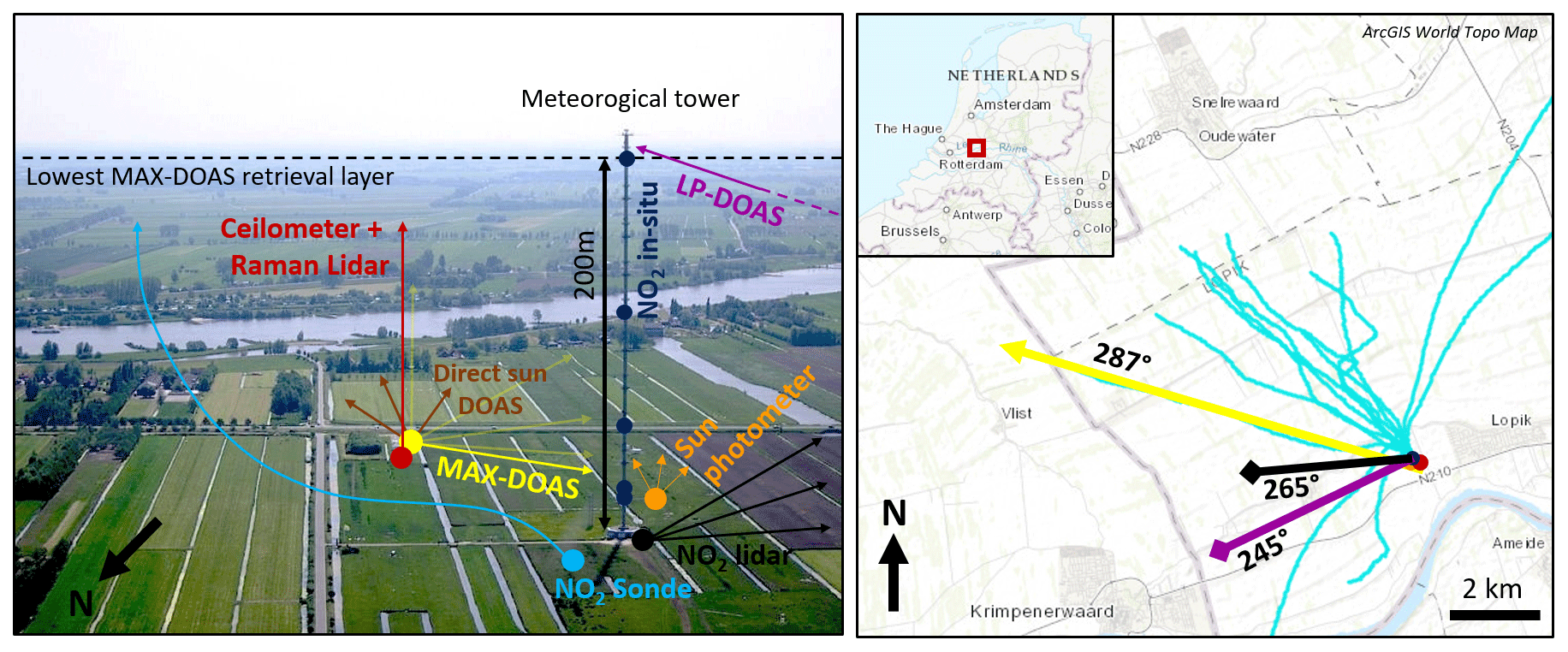
Figure 1 Left: image of the CESAR site with position and approximate viewing directions of the MAX-DOAS instruments and supporting observations of relevance for this study. Right: map with instrument locations, viewing geometries and sonde flight paths indicated (credit: Esri 2018).

2.1 MAX-DOAS dataset

2.1.1 Underlying dSCD dataset

Deriving vertical gas concentration and aerosol extinction profiles from scattered skylight spectra can be regarded as a two-step process: the first step is the DOAS spectral analysis, where the magnitude of characteristic absorption patterns of different gas species in the recorded spectra is quantified to derive the so-called “differential slant column densities” (dSCDs; definition in the following paragraph). These provide information on integrated gas concentrations along the lines of sight. The second step is the actual profile retrieval, where inversion algorithms incorporating atmospheric radiative transfer models (RTMs) are applied to retrieve concentration profiles from the dSCDs derived in the first step.

The very initial data in the MAX-DOAS processing chain are intensities of scattered skylight I_λ(α) at different wavelengths λ (ultraviolet and visible spectral ranges, typical resolutions of 0.5 to 1.5 nm) recorded under different viewing elevation angles α (ideally the telescope's FOV is negligible compared to the elevation angle resolution). Along the light path l from the top of the atmosphere (TOA) to the instrument on the ground, each atmospheric gas species i imprints its unique spectral absorption pattern (given by the absorption cross section σ_i,λ) onto the TOA spectrum I_λ,TOA with the optical thickness

$$\begin{array}{}\text{(1)}& {\mathit{\tau }}_{\mathit{\lambda }}\left(\mathit{\alpha }\right)=\log \left({\displaystyle \frac{I_{\mathit{\lambda },\mathrm{TOA}}}{I_{\mathit{\lambda }}\left(\mathit{\alpha }\right)}}\right)=\sum _i{\mathit{\sigma }}_{i,\mathit{\lambda }}{S}_i\left(\mathit{\alpha }\right)+C.\end{array}$$

S_i(α) is the slant column density (SCD), which is the trace gas concentration integrated along l. C represents terms accounting for other instrumental and physical effects than trace gas absorption (for instance, scattering on molecules and aerosols) that will not be further discussed in this context. S_i(α) is inferred by spectrally fitting literature values of σ_i,λ to the observed τ_λ(α). Since normally I_λ,TOA is not available for the respective instrument, optical thicknesses are instead assessed with respect to the spectrum recorded in zenith viewing direction to obtain

$$\begin{array}{}\text{(2)}& \mathrm{\Delta }{\mathit{\tau }}_{\mathit{\lambda }}\left(\mathit{\alpha }\right)=\log \left({\displaystyle \frac{I_{\mathit{\lambda }}(\mathit{\alpha }=\mathrm{90}{}^{\circ })}{I_{\mathit{\lambda }}\left(\mathit{\alpha }\right)}}\right).\end{array}$$

Then the spectral fit yields the so-called differential slant column densities (dSCDs):

$$\begin{array}{}\text{(3)}& \mathrm{\Delta }S\left(\mathit{\alpha }\right)=S\left(\mathit{\alpha }\right)-S(\mathit{\alpha }=\mathrm{90}{}^{\circ }),\end{array}$$

which are the typical output of the DOAS spectral analysis when applied to MAX-DOAS data. For further details on the DOAS method, refer to Platt and Stutz (2008).

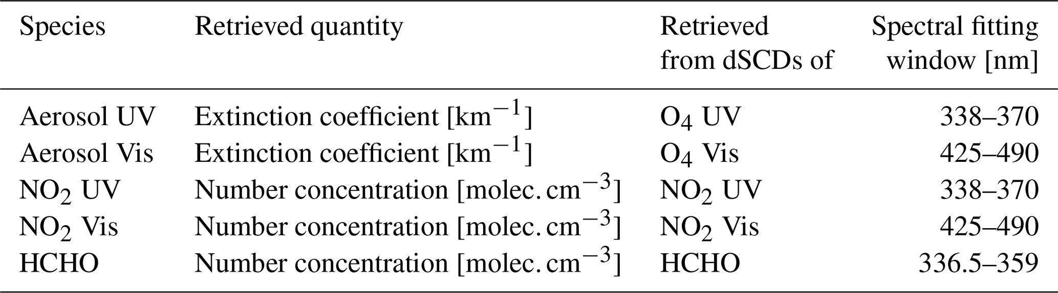
During the CINDI-2 campaign, each participant measured spectra with their own instrument and derived dSCDs applying their preferred DOAS spectral analysis software. The pointings (azimuthal and elevation) of all MAX-DOAS instruments were aligned to a common direction (Donner et al., 2019) and all participants had to comply with a strict measurement protocol, assuring synchronous pointing and spectra acquisition under highly comparable conditions (Apituley et al., 2020). A detailed comparison and validation of the dSCD results was conducted by Kreher et al. (2019). In the course of their study, Kreher et al. (2019) identified the most reliable instruments to derive a “best” median dSCD dataset. This dataset – in the following referred to as the “median dSCDs” – was distributed among the participants. All participants used the median dSCDs as the input data for their retrieval algorithms and retrieved the profiles that are compared in this study. The “median dSCD” approach was chosen for the following reasons: (i) it enables us to compare the profiling algorithms independently from differences in the input dSCDs, which is necessary to assess the individual algorithm performance; (ii) it makes this study directly comparable to the report by Frieß et al. (2019). Among others, this allows us to assess to what extent MAX-DOAS profiling studies on synthetic data (with lower effort) can be used to substitute studies on real data. (iii) Two decoupled studies are obtained (Kreher et al., 2019 and this study), each confined to a single step in the MAX-DOAS processing chain (the DOAS spectral analysis to obtain dSCDs and the actual profile inversion). A disadvantage of the median dSCD approach is that the reliability of a typical MAX-DOAS observation undergoing the whole spectra acquisition and processing chain cannot be assessed. Therefore, a comparison of profiles retrieved with the participant's own dSCDs was also conducted but is not a substantial part of this study. However, these results and a corresponding short discussion can be found in Supplement Sect. S10 and Sect. 3.7, respectively. The median dSCDs cover the campaign core period from 12 to 28 September 2016, considering only data from the first 10 min of each hour between 07:00 and 16:00 UT, where the CINDI-2 MAX-DOAS measurement protocol scheduled an elevation scan in the nominal 287^∘ azimuth viewing direction with respect to the north. Hence, the total number of processed elevation scans was 170. An elevation scan consisted of 10 successively recorded spectra at viewing elevation angles α of 1, 2, 3, 4, 5, 6, 8, 15, 30 and 90^∘, at an acquisition time of 1 min each. dSCDs were provided for three chemical species, namely O₄, NO₂ and HCHO. O₄ and NO₂ were each provided for two different spectral fitting ranges, in the UV and Vis spectral regions, resulting in five data products (see Table 1). From the median dSCDs, the participants retrieved profiles for the species listed in Table 1. Not all participants retrieved all species and therefore do not necessarily appear in all plots.

Table 1 List of the retrieved species and fitting ranges. For further details on the spectral analysis, please refer to Kreher et al. (2019).

2.1.2 Participating groups and algorithms

Table 2 lists the compared algorithms including the underlying method (OEM, PAR or ANA) and the participating groups with corresponding labels and plotting symbols as they are used throughout the comparison. OEM and PAR algorithms rely on the same idea: a layered horizontally homogeneous atmosphere is set up in a RTM with distinct parameters (aerosol extinction coefficient, trace gas amounts, temperature, pressure, water vapour and aerosol properties) attributed to each layer. This model atmosphere is then used to simulate MAX-DOAS dSCDs under consideration of the viewing geometries. To retrieve a profile from the measured dSCDs, the model parameters are optimized to minimize the difference between the simulated and measured dSCDs based on a predefined cost function.

Regarding profiles, typically only 2 to 4 degrees of freedom for signal (DOFS or p) can be retrieved from MAX-DOAS observations, such that general profile retrieval problems with more than p independent retrieved parameters are ill-posed and prior information has to be assimilated to achieve convergence. For OEM algorithms, this is provided in the form of an a priori profile and associated a priori covariance (Rodgers, 2000), defining the most likely profile and constraining the space of possible solutions according to prior experience. They constitute a portion of the OEM cost function such that with decreasing information contained in the measurements, layer concentrations are drawn towards their a priori values. PAR algorithms implement prior assumptions by only allowing predefined profile shapes which can be described by a few parameters.

For OEM algorithms, the radiative transport simulations are performed online in the course of the retrieval, whereas the PAR algorithms in this study rely on look-up tables, which are precalculated for the parameter ranges of interest. Therefore, PAR algorithms are typically faster than OEM algorithms but also require more memory. The ANA approach by NASA was developed as a quick-look algorithm and assumes a simplified radiative transport, based on trigonometric considerations. Since the model equations can be solved analytically for the parameters of interest, neither radiative transport simulation nor the calculation of look-up tables is necessary, and an outstanding computational performance is achieved compared to other algorithms (factor of ≈10³ in processing time; see Frieß et al., 2019).

For further descriptions of the methods and the individual algorithms, please refer to Frieß et al. (2019). Besides the algorithms described therein, our study includes results from the M³ algorithm by LMU (see Table 2 for definition). Its description can be found in Supplement Sect. S1. For details, refer to the references given in Table 2.

Note that two versions of aerosol results from the MAPA algorithm (see Table 2 for definition) with different O₄ scaling factors (SFs) are discussed within this paper, referred to as mp-0.8 (retrieved with SF=0.8) and mp-1.0 (SF=1.0), respectively. The scaling factor is applied to the measured O₄ dSCDs prior to the retrieval and was initially motivated by previous MAX-DOAS studies which reported a significant yet debated mismatch between measured and simulated dSCDs (e.g. Wagner et al., 2009; Clémer et al., 2010; Ortega et al., 2016; Wagner et al., 2019, and references therein). Also for MAPA during CINDI-2, a scaling factor of 0.8 was found to improve the dSCD agreement, enhance the number of valid profiles and significantly improve the agreement with the Sun photometer aerosol optical thickness (Beirle et al., 2019). However, in the course of this study, it was found that for OEM algorithms the disagreement between Sun photometer and MAX-DOAS can largely be explained by smoothing effects (see Sect. 3.4) and that (at least averaged over campaign) there are no clear indications that a SF is necessary (see Supplement Sect. S2).

Table 2 Groups who retrieved and provided profiling results for this study.

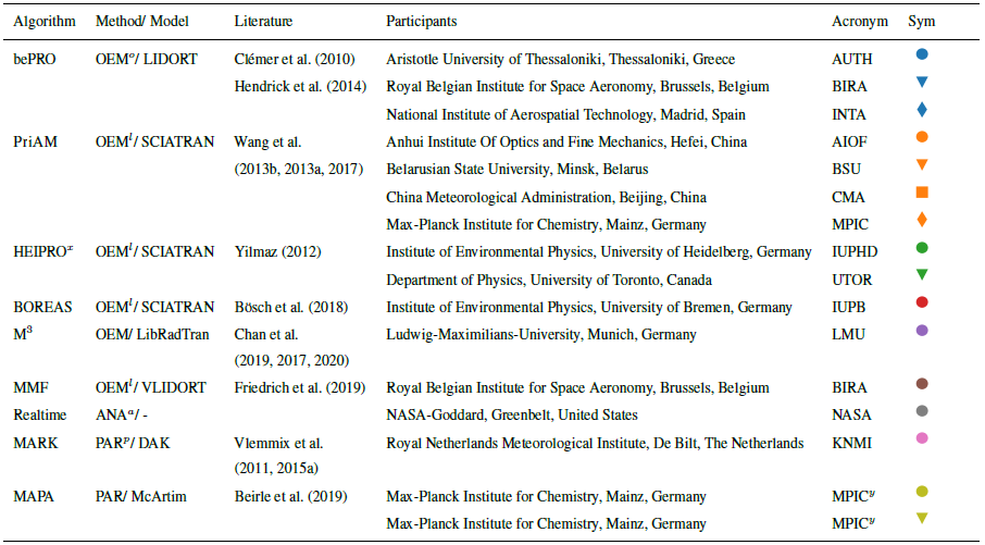
^o OEM: optimal estimation. ^a ANA: analytical approach without radiative transfer model. ^p PAR: parameterized approach. ^x IUPHD and UTOR used different versions of HEIPRO (1.2 and 1.5/1.4, respectively). ^y Two versions of MAPA (labelled mp-10 and mp08) with different O₄ scaling factors (0.8 and 1.0) are included in the comparison. ^l Aerosol extinction is retrieved in logarithmic space. This removes negative values and allows larger values.

2.1.3 Retrieval settings

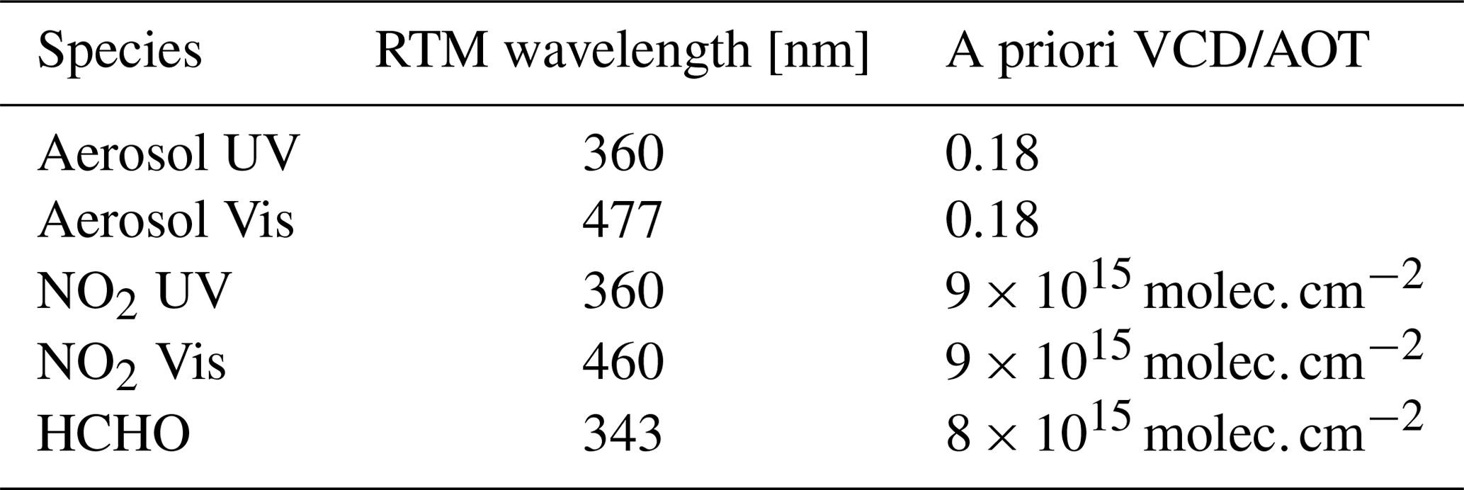
To reduce possible sources of discrepancies, all profiles shown in this study were retrieved according to predefined settings similar to those of the intercomparison study by Frieß et al. (2019): pressure, temperature, total air density and O₃ vertical profiles between 0 and 90 km altitude were averaged from O₃ sonde measurements performed in De Bilt by KNMI during September months of the years 2013–2015. A fixed altitude grid was used for the inversion, consisting of 20 layers between 0 and 4 km altitude, each with a height of Δh=200 m. The results of the parameterized approaches and OEM algorithms where the exact grid could not readily be applied during inversion were interpolated and averaged accordingly afterwards. Note that, for radiative transfer simulations, the atmosphere was represented by finer (25 to 100 m) layers close to the surface, increasing with altitude) and farther extending (up to 40 to 90 km altitude) grids, inherently defined by the individual retrieval algorithms. Surface and instruments' altitudes were fixed to 0 m, which is close to the real conditions: the CESAR site and most of the surrounding area lie at 0.7 m b.s.l., whereas the instruments were installed at 0 to 6 m above sea level. The model wavelengths were fixed according to Table 3. In the case of the HCHO retrieval, the aerosol profiles retrieved at 360 nm were extrapolated to 343 nm using the mean Ångström exponent for the 440–675 nm wavelength range derived from Sun photometer measurements (see Sect. 2.2.1) on 14 September 2016 in Cabauw. For the aerosol parameters, the single scattering albedo was fixed to 0.92 and the asymmetry factor to 0.68 for both 360 and 477 nm. These are mean values for 14 September 2016 derived from Aerosol Robotic Network (AERONET) measurements at 440 nm in Cabauw. The standard CINDI-2 trace gas absorption cross sections were applied (see Kreher et al., 2019). Scaling of the measured O₄ dSCDs prior to the retrieval was not applied. An exception is the parameterized MAPA algorithm for which two datasets, one without and one with a scaling (SF=0.8), were included in this study. The OEM a priori profiles for both aerosol and trace gas retrievals were exponentially decreasing profiles with a scale height of 1 km and aerosol optical thicknesses (AOTs) and vertical column densities (VCDs) as given in Table 3. For the AOTs, the mean value at 477 nm for the first days of September 2016 derived from AERONET measurements are used. Trace gas VCDs are mean values derived from Ozone Monitoring Instrument (OMI) observations in September 2006–2015. A priori variance and correlation length were set to 50 % and 200 m, respectively.

Table 3 Prescribed settings for the radiative transfer simulation wavelengths and a priori total columns (OEM algorithms only).

2.1.4 Requested dataset

All participants were requested to submit the following results of their retrieval: (i) profiles and profile errors, optionally with errors separated into contributions from propagated measurement noise and smoothing effects; (ii) modelled dSCDs as calculated by the RTM for the retrieved atmospheric state; (iii) averaging kernels (AVKs) for assessment of information content and vertical resolution (only available for OEM approaches); (iv) optional flags, giving participants the opportunity to mark profiles as invalid. The flagging must be based on inherent quality indicators, which typically are the root-mean-square difference between measured and modelled dSCDs or the general plausibility of the retrieved profiles. Note that only four institutes submitted flags (INTA/bePRO, BIRA/bePRO, KNMI/MARK and MPIC/MAPA). It is assumed that an accurate aerosol retrieval is necessary to infer light path geometries; thus, trace gas profiles are generally considered invalid if the underlying aerosol retrieval is invalid. A detailed description of the flagging criteria and flagging statistics can be found in Supplement Sect. S3.

2.2 Supporting observations

This section introduces the supporting observations that were used for comparison and validation of the MAX-DOAS retrieved results. It shall be pointed out that a general challenge here was to find compromises between (i) using only accurate and representative data with good spatiotemporal overlap and (ii) keeping as much supporting data as possible to have a large comparison dataset. Considerations and investigations on this issue (e.g. comparisons between the supporting observations, spatiotemporal variability and overlap) which lead to the decisions finally taken are mentioned in the following subsections and described in more detail in the Supplement they refer to.

2.2.1 Aerosol optical thickness

Independent aerosol optical thickness measurements τ_aer were performed with a Sun photometer (CE318-T by Cimel) located close to the meteorological tower of the CESAR site (see Fig. 1), which is part of AERONET (see Holben et al., 1998). AOTs were derived from direct-sun radiometric measurements in ≈ 15 min intervals at 1020, 870, 675 and 440 nm wavelength. The AERONET level 2.0 data were used, which are cloud screened, recalibrated and quality filtered (according to Smirnov et al., 2000). For the extrapolation of τ_aer to the DOAS retrieval wavelengths of 360 and 477 nm, a dependency of τ_aer on the wavelength λ according to

$$\begin{array}{}\text{(4)}& \ln {\mathit{\tau }}_{\mathrm{s}}\left(\mathit{\lambda }\right)={\mathit{\alpha }}_{\mathrm{0}}+{\mathit{\alpha }}_{\mathrm{1}}\cdot \ln \mathit{\lambda }+{\mathit{\alpha }}_{\mathrm{2}}\cdot (\ln \mathit{\lambda }{)}^{\mathrm{2}}\end{array}$$

was assumed, following Kaskaoutis and Kambezidis (2006). The parameters α_i were retrieved by fitting Eq. (4) to the available data points. Note that α₁ corresponds to the Ångström exponent when only the first two (linear) terms on the right-hand side are used. The last quadratic term enables us to additionally account for a change of the Ångström exponent with wavelength. For the linear temporal interpolation to the MAX-DOAS profile timestamps, the maximum interpolated data gap was set to 30 min, resulting in a data coverage of about 30 %. Smirnov et al. (2000) propose a Sun photometer total accuracy in τ_s of 0.02. Each AOT is actually an average over three subsequently performed measurements. In this study, the proposed accuracy of 0.02 was enhanced by the variability between them (typically on the order of 0.008).

2.2.2 Aerosol profiles

Information on the aerosol extinction coefficient profiles (in the following referred to as “aerosol profiles”) was obtained by combining the Sun photometer AOT with data from a ceilometer (Lufft CHM15k Nimbus). The latter continuously provided vertically resolved information on the atmospheric aerosol content by measuring the intensity of elastically backscattered light from a pulsed laser beam (1064 nm) propagating in zenith direction (see, e.g. Wiegner and Geiß, 2012). The raw data are attenuated backscatter coefficient profiles over an altitude range from 180 m to 15 km, with a temporal and vertical resolution of 12 s and 10 m, respectively. These were converted to extinction coefficient profiles by scaling with simultaneously measured Sun photometer or MAX-DOAS AOTs. This is described in detail in Supplement Sect. S4.1. Note that the approach described there presumes a constant extinction coefficient for altitudes ≤180 m and that the aerosol properties like size distribution, single scattering albedo and shape remain constant with altitude. To check plausibility, Supplement Sect. S4.1 compares the resulting profiles at 360 nm to a few available extinction coefficient profiles, measured by a Raman lidar at 355 nm (the CESAR Water Vapor, Aerosol and Cloud Lidar “CAELI”, operated within the European Aerosol Research lidar Network (EARLINET; Bösenberg et al., 2003; Pappalardo et al., 2014) and described in detail in Apituley et al., 2009). The average root-mean-square difference (RMSD) between scaled ceilometer and Raman lidar profiles up to 4 km altitude is $\approx \mathrm{0.03}{\mathrm{km}}^{-\mathrm{1}}$. However, since there are only few Raman lidar validation profiles available and only for altitudes > 1 km, the ceilometer aerosol profiles should be consulted for qualitative comparison only.

2.2.3 NO₂ profiles

NO₂ profiles were recorded sporadically by two measurement systems: radiosondes (described in Sluis et al., 2010) and an NO₂ lidar (Berkhout et al., 2006). Radiosondes were launched at the CESAR measurement site during the campaign. For this study, only data from sonde ascents through the lowest 4 km (which is the MAX-DOAS profiling retrieval altitude range) were used. A sonde profile was considered temporally coincident to a MAX-DOAS profile, when the middle timestamps of MAX-DOAS elevation scan and sonde flight were less than 30 min apart. The horizontal sonde flight paths are indicated in Fig. 1. Typical flight times (lowest 4 km) were of the order of 10–15 min. Data were recorded at a rate of 1 Hz, typically resulting in a vertical resolution of approximately 10 m at an approximate measurement uncertainty in NO₂ concentration of $\mathrm{5}\times {\mathrm{10}}^{\mathrm{10}}\mathrm{molec}.{\mathrm{cm}}^{-\mathrm{3}}$. The horizontal travel distances varied strongly between 4 and 18 km. A detailed overview of the flights is given in Supplement Sect. S4.2.

The NO₂ lidar is a mobile instrument setup inside a lorry which was located close to the CESAR meteorological tower. It combines lidar observations at different viewing elevation angles to enhance vertical resolution and to obtain sensitivity close to the ground, despite the limited range of overlap between sending and receiving telescope (see also Sect. 2.2.2). The instrument is sensitive along its line of sight from 300 to 2500 m distance to the instrument. The azimuthal pointing was 265^∘ with respect to the north, and the operational wavelength is 413.5 nm. Typical specified uncertainties in the retrieved concentrations are around $\mathrm{2.5}\times {\mathrm{10}}^{\mathrm{10}}\mathrm{molec}.{\mathrm{cm}}^{-\mathrm{3}}$. Profiles were provided at a temporal resolution of 28 min, each profile consisting of a series of (occasionally overlapping) altitude intervals with constant gas concentration. For an exemplary profile and details on its conversion to the MAX-DOAS retrieval altitude grid, please refer to Supplement Sect. S4.3. A lidar profile was considered temporally coincident to a MAX-DOAS profile, when the middle timestamps of MAX-DOAS elevation scan and lidar profile were less than 30 min apart. This resulted in 25 suitable lidar profiles recorded on six different days during the campaign. Example profiles of both radiosonde and NO₂ lidar are shown in the course of a comparison between the two observations in Supplement Sect. S4.5.

2.2.4 Trace gas vertical column densities

Tropospheric trace gas VCDs were derived from direct-sun DOAS observations, which were performed between minutes 40 and 45 of each hour. NO₂ VCDs were retrieved from combined datasets of two Pandora DOAS instruments (instrument numbers 31 and 32) and calculated based on the Spinei et al. (2014) approach. The reference spectrum was created from the spectra with lowest radiometric error over the whole campaign and the residual NO₂ signal was determined by applying the so-called minimum Langley extrapolation (Herman et al., 2009). The temperature dependence of the NO₂ cross sections was used to separate the tropospheric from the stratospheric column.

HCHO VCDs were retrieved from data of the BIRA DOAS instrument (number 4). A fixed reference spectrum acquired on 18 September 2016 at 09:41 UTC and 55.6^∘ SZA was used. DOAS fitting settings were identical to those used for the CINDI-2 HCHO dSCD intercomparison (Kreher et al., 2019). The residual amount of HCHO in the reference spectrum of $(\mathrm{8.8}\pm \mathrm{1.6})\times {\mathrm{10}}^{\mathrm{15}}\mathrm{molec}.{\mathrm{cm}}^{-\mathrm{2}}$ was estimated using a MAX-DOAS profile retrieved on the same day and a geometrical air mass factor (AMF) corresponding to 55.6^∘ SZA. Because of that, the HCHO VCDs cannot be considered as a fully independent dataset. VCDs were calculated from total HCHO slant column densities (SCDs) using a geometrical AMF including a simple correction for the Earth's sphericity. Only spectra with DOAS fit residuals $<\mathrm{5}\times {\mathrm{10}}^{-\mathrm{4}}$ were considered as valid direct-sun data. As for AOTs, these observations can only be performed when the Sun is clearly visible; hence, the coverage for cloudy scenarios is scarce.

2.2.5 Trace gas surface concentrations

Note that in the following, “surface concentration” will not refer to measurements in the very proximity to the ground but to the average concentration in the lowest 200 m of the atmosphere, as retrieved for the MAX-DOAS first profile layer. Trace gas surface concentrations of HCHO and NO₂ were provided by a long-path DOAS system operated by IUP-Heidelberg (LP-DOAS; see Pikelnaya et al., 2007; Pöhler et al., 2010; Merten et al., 2011; Nasse et al., 2019). The LP-DOAS system consists of a light-sending and receiving telescope unit located at 3.8 km horizontal distance to a retro reflecting mirror mounted at the top (207 m altitude) of the meteorological tower (see Supplement Sect. S4.4). Light from a UV–Vis light source is sent by the telescope to the retroreflector and the reflected light is again received by the telescope unit and spectrally analysed applying the DOAS method. The fundamental difference to the MAX-DOAS instruments is the well-defined light path which enables very accurate determination of trace gas mixing ratios, averaged along the line of sight. Accordingly, with the retroreflector mounted at 207 m altitude, one obtains average mixing ratios over the lowest MAX-DOAS retrieval layer, as indicated in Fig. 1. Considering DOAS fitting errors and uncertainties in the applied literature cross sections (Vandaele et al., 1998; Meller and Moortgat, 2000; Pinardi et al., 2013) yields an average accuracy of the LP-DOAS of $\pm \mathrm{1.5}\times {\mathrm{10}}^{\mathrm{9}}\mathrm{molec}.{\mathrm{cm}}^{-\mathrm{3}}\pm \mathrm{3}\mathit{\%}$ ($\pm \mathrm{5}\times {\mathrm{10}}^{\mathrm{9}}\mathrm{molec}.{\mathrm{cm}}^{-\mathrm{3}}\pm \mathrm{9}$ %) for NO₂ (HCHO), respectively. Given the high accuracy, the total vertical coverage of the surface layer and a near-continuous dataset over the campaign period, the LP-DOAS provides the most reliable dataset for the validation of CINDI-2 MAX-DOAS trace gas profiling results.

Further observations for qualitative validation are the surface values of the NO₂ lidar and the radiosondes and also in situ monitors in the CESAR meteorological tower. Teledyne in situ NO₂ monitors (Teledyne API, model M200E) were located in the tower basement and were subsequently connected to different inlets located at 20, 60, 120 and 200 m altitude (switching intervals approx. 5 min). Further, a CAPS (type AS32M, based on attenuated phase shift spectroscopy, Kebabian et al., 2005) and a CE-DOAS (cavity-enhanced DOAS; Platt et al., 2009 and Horbanski et al., 2019) were continuously measuring at 27 m altitude. All the in situ measurements at the tower were combined to obtain another set of surface concentration measurements, more representative of concentrations close to the site. The data were combined by linearly interpolating over altitude between the instruments and subsequently averaging the resulting profile over the retrieval surface layer (0–200 m altitude). Note that this method gives a large weight to the uppermost measurements, as they are representative of the majority of the relevant layer.

2.2.6 Meteorology

Meteorological data for the surface layer (pressure, temperature and wind information) routinely measured at the CESAR site were taken from the CESAR database (CESAR, 2018) at a temporal resolution of 10 min. Cloud conditions were retrieved from MAX-DOAS data of instruments 4 and 28 according to the cloud classification algorithm developed by MPIC (Wagner et al., 2014; Wang et al., 2015). Basically, only two cloud condition states are distinguished in the statistical evaluation: “clear-sky” (green) and “presence of clouds” (red). Only in the overview and correlation plots, “presence of clouds” is further subdivided into “optically thin clouds” (orange) and “optically thick clouds” (red). According to this classification, 72 (98) of the 170 profiles were measured under clear-sky (cloudy) conditions. Over the whole campaign, there was only one rain event (precipitation > 0.01 mm) coinciding with the measurements on 25 September 2016 between 15:00 and 17:00 UT. At forenoon on 16 September, a heavy fog event strongly limited the visibility (see also Supplement Sect. S5).

2.3 Comparison strategy

2.3.1 General approach

Different MAX-DOAS retrieval algorithms were extensively compared in Frieß et al. (2019) using synthetic data. The crucial differences of the presented study are that (i) the underlying spectra are not synthetic but were recorded with real instruments, meaning that real noise and instrument artefacts propagate into the results. (ii) Independent information on the real profile can only be inferred from supporting observations with their own uncertainties and an imperfect spatiotemporal overlap with the MAX-DOAS measurements. (iii) The real conditions encountered can exceed the model's scope because horizontal inhomogeneities or the fact that many of the fixed forward model input parameters (such as aerosol properties, surface albedo, temperature and pressure profiles) are averaged quantities of former observations which might be inaccurate for specific days and conditions. (iv) In some cases, different participants used the same retrieval algorithms; this allows an assessment of the impact of different settings in the remaining parameters, which were not prescribed (see Sect. 2.1.3). The approaches chosen here are therefore limited to the examination of (i) the consistency among the participants, (ii) the consistency of the results with available supporting observations and (iii) inherent quality proxies of the retrieval (described in the next paragraph). Table 4 summarizes the quantities which are compared, together with the corresponding supporting observations if available.

Table 4 Overview of compared quantities and available supporting data.

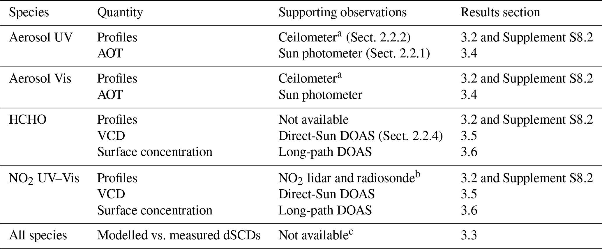
^a Elastic backscatter profiles scaled with the Sun photometer or MAX-DOAS AOT. ^b Scarce data coverage. ^c Inherent quality proxy.

In this study, agreement between different observations is statistically assessed by (i) weighted RMSDs, (ii) weighted “bias” as introduced below and (iii) weighted least-squares regression analysis. Discussions and summary are focused on RMSD, being the most fundamental quantity as it represents both statistical and systematic deviations. The bias was introduced as a general proxy for systematic deviations. Correlation coefficient, slope and offset from the regression analysis are provided and consulted for a more differentiated view.

Consider two time series of length N_T: the retrieval result x_p,t of a participant p at time t and some reference observation x_ref,t (either MAX-DOAS median results or data from supporting observations, as further described below) with associated uncertainties σ_p,t and σ_ref,t. Then the RMSD is defined as

$$\begin{array}{}\text{(5)}& \text{RMSD:}{\mathit{\sigma }}_{\mathrm{rms},p}=\sqrt{{\displaystyle \frac{\mathrm{1}}{N_T}}\cdot {\displaystyle \frac{\mathrm{1}}{{\sum }_t{w}_t}}\cdot \sum _t{w}_t{\left(x_{p,t}-x_{\mathrm{ref},t}\right)}^{\mathrm{2}}}.\end{array}$$

The weights w_t are defined according to

$$\begin{array}{}\text{(6)}& w_t={\displaystyle \frac{\mathrm{1}}{{\mathit{\sigma }}_{p,t}^{\mathrm{2}}+{\mathit{\sigma }}_{\mathrm{ref},t}^{\mathrm{2}}}}\end{array}$$

and are also applied for the bias calculation and regression analysis. The bias is defined as

$$\begin{array}{}\text{(7)}& \text{bias:}{\mathit{\sigma }}_{\mathrm{bias},p}={\displaystyle \frac{\mathrm{1}}{N_T}}\cdot {\displaystyle \frac{\mathrm{1}}{{\sum }_t{w}_t}}\cdot \sum _t{w}_t\left(x_{p,t}-x_{\mathrm{ref},t}\right).\end{array}$$

Sometimes, the term “average RMSD” (“average bias”) is used, which refers to the average over the RMSD (bias) values of the individual participants. We further introduce the “average bias magnitude” that averages the absolute values of the bias. When referring to “relative RMSDs” (“relative bias”), the underlying RMSD (bias) value was divided by the average of the investigated quantity. For the linear regression analysis, the vertical distance between the model and the data points is minimized and also here the weights w_t are applied.

To assess the consistency among the participants, the median result over the valid profiles of all participants is inserted as x_ref,t. The median is used instead of the mean value, since it is less sensitive to (sometimes unphysical) outliers. This comparison shows how far the choice of the retrieval algorithm or technique affects the results but it does not reveal general systematic MAX-DOAS retrieval errors. Outliers observed for distinct participants and algorithms are therefore not necessarily an indicator for poor performance.

To assess the consistency with supporting observations, the latter are inserted as x_ref,t. This comparison is a better indicator for the real retrieval performance. However, uncertainties of supporting instruments (see Supplement Sect. S4.5), smoothing effects (see Sect. 2.3.2) and imperfect spatial and temporal overlap of the different observations (see Sect. 2.3.3) complicate the interpretation.

An inherent quality indicator for the retrieval algorithms is the consistency of modelled and measured dSCDs. During the inversion, the goal is to minimize the deviation between the RTM-simulated dSCDs and the actually measured ones. If strong deviations remain after the final iteration in the minimization process, this indicates failure of the retrieval.

In a few cases (e.g. Sect. 3.2, where full profiles are compared), the scatter among several participants p (of number N_P) and several retrieval layers h (of number N_H) is of interest. For this purpose, we define the “average standard deviation” (ASDev) which is the standard deviation observed among the participants for individual profiles averaged over retrieval layers and time; hence,

$$\begin{array}{}\text{(8)}& \begin{array}{rl}\text{ASDev:}{\mathit{\sigma }}_{\mathrm{asdev}}=& {\displaystyle \frac{\mathrm{1}}{N_T}}\sum _t\\ & {\displaystyle \frac{\mathrm{1}}{N_H}}\sum _h\sqrt{{\displaystyle \frac{\mathrm{1}}{N_P-\mathrm{1}}}\sum _p{\left(x_{p,h,t}-{\overline{x}}_{h,t}\right)}^{\mathrm{2}}},\end{array}\end{array}$$

with ${\overline{x}}_{h,t}$ being the average (over participants) MAX-DOAS retrieved concentration for a given time t and layer h. If not stated otherwise, ASDev values of profiles are calculated considering the lowest five retrieval layers (up to 1 km altitude).

In the statistical evaluations, clear-sky and cloudy conditions as well as unfiltered and filtered data (according to the flags provided by the participants) are distinguished. The distinction between cloud conditions is of major importance, as particularly in the case of aerosol retrievals under broken clouds, the quality of the results is typically strongly degraded. A consequence of regarding these data subsets is that the number of contributing data points not only depends on the number of submitted profiles and the number of coincident data points from supporting observations but further on the filter settings. Any regression RMSD or bias value with less than five contributing data points is considered to be statistically unrepresentative and is omitted. If not stated otherwise, numbers given in the text were calculated considering valid data only.

2.3.2 Smoothing effects

As shown in Sect. 3.1 below, in particular in the UV range, the sensitivity of ground-based MAX-DOAS observations decreases rapidly with altitude, meaning that species above ≈2 km typically cannot be reliably quantified. At higher altitudes, OEM retrieval results are drawn towards the a priori profile (according to the definition of the cost function; see Rodgers, 2000), while the results of parameterized and analytical approaches are driven by the chosen parametrization and their implementation. Further, the vertical resolution is limited (from 100 to several hundred metres, increasing with altitude), which affects the profile shape and – of most importance in this study – the retrieved surface concentration. Both effects cause deviations from the true profile that are in the following referred to as “smoothing effects”.

For a meaningful quantitative comparison, they should be considered. This is possible for OEM retrievals, where the information on the vertical resolution and sensitivity is given by the averaging kernel matrix (AVK; see Sect. 3.1 for details). For a meaningful quantitative comparison of an OEM-retrieved profile and a validation profile x (assumed here to perfectly represent the true state of the atmosphere), the validation profile resolution and information content has to be degraded by “smoothing” it with the corresponding MAX-DOAS AVK matrix A according to the following equation (Rodgers and Connor, 2003; Rodgers, 2000):

$$\begin{array}{}\text{(9)}& \stackrel{\mathrm{̃}}{\mathit{x}}=\mathbf{A}\mathit{x}+(\mathbf{1}-\mathbf{A}){\mathit{x}}_a.\end{array}$$

Here, x_a is the a priori profile and $\stackrel{\mathrm{̃}}{\mathit{x}}$ represents the profile that a MAX-DOAS OEM retrieval (with the resolution and sensitivity described by A) would yield in the respective scenario. For layers with high (low) gain in information, $\stackrel{\mathrm{̃}}{\mathit{x}}$ is drawn towards x (x_a), while vertical resolution is degraded if A has significant off-diagonal entries (compare to Sect. 3.1). In this study, this has implications not only for the comparison of profiles but also the comparison of the total columns (AOTs and VCDs, which are derived simply by vertical integration of the corresponding profiles) and surface trace gas concentrations. For total columns, the dominant issue is the lack of information at higher altitudes. In contrast, there is reasonable information on the surface concentration; however, smoothing can have a severe impact here in the case of strong concentration gradients close to the surface. The impact on the individual observations is discussed in the corresponding sections below. A particularly important consequence of smoothing effects is the “partial AOT correction” (PAC), which is introduced and discussed in Sect. 3.4.

Finally, it shall be pointed out that the sensitivity and spatial resolution are strongly affected by the exact approach that is chosen to solve the ill-posed inversion problem. Frieß et al. (2006), for instance, demonstrates that the sensitivity to higher altitudes can be enhanced by relaxing the prior constraints and by retrieving profiles at several wavelengths simultaneously.

2.3.3 Spatiotemporal variability

It is obvious already from Fig. 1 and Sect. 2.2 that the MAX-DOAS instruments and the various supporting observations sample different air volumes at different times. In addition, the MAX-DOAS horizontal viewing distance (derived in Supplement Sect. S5) is highly variable, changing between 2 and 30 km during the campaign for the lowest viewing elevation angles. Similar investigations were already performed by Irie et al. (2011) using CINDI-1 data; however, they used a different definition of the viewing distance. Table S6 summarizes the spatial and temporal mismatches between MAX-DOAS and supporting observations. Spatial mismatches are of the order of 10 km; temporal mismatches vary between 0 and 20 min. Consequently, strong spatiotemporal variations of the observed quantities are expected to induce large discrepancies among the observations, independent of the data quality. Quantitative estimates of the impact on the comparison could only be derived for NO₂ surface concentrations and under strong simplifications (for details, see Supplement Sect. S6), yielding an RMSD of $\mathrm{3.5}\times {\mathrm{10}}^{\mathrm{10}}\mathrm{molec}.{\mathrm{cm}}^{-\mathrm{3}}$. This is indeed of similar magnitude as the average RMSD observed during the comparison (approx. $\mathrm{5}\times {\mathrm{10}}^{\mathrm{10}}\mathrm{molec}.{\mathrm{cm}}^{-\mathrm{3}}$). It shall further be noted that under strong spatial variability the horizontal homogeneity assumed by the retrieval forward models is inaccurate.

3 Comparison results

3.1 Information content

In the case of OEM retrievals, the gain in information on the atmospheric state can be quantified according to Rodgers (2000). Essentially speaking, this is done by comparing the knowledge before (represented by the a priori profile and its uncertainties) and after the profile retrieval. The gain in information for each individual vertical profile can be represented by the AVK matrix (denoted by A). A_ij describes the sensitivity of the measured concentration in the ith layer to small changes in the real concentration in the jth layer. Each row A_i can thus be plotted over altitude providing the following information: (1) the value in the layer i itself (the diagonal element A_ii with a value between 0 and 1) gives the gain in information while 1−A_ii represents the amount of a priori knowledge which had to be assimilated to obtain a well-defined concentration value. (2) The values in the other layers (off-diagonal elements of A) indicate the cross sensitivity of layer i to layer j. Typically, the cross sensitivity decreases with the distance to the layer i. The length of this decay (note that i can be converted to the corresponding altitude by multiplication with the retrieval layer thickness Δh) is an indicator for the vertical resolution of the retrieval. The trace of A is equal to the DOFS and hence the total number of independent pieces of information gained from the measurements compared to the a priori knowledge. Figure 2 visualizes the average AVK matrices (median over participants and mean over time) for all five species studied in this work. Note that the AVKs do not necessarily represent the real or total sensitivity and information content of MAX-DOAS observations as they only consider the gain of information with respect to the a priori knowledge. Hence, for stricter a priori constraints, less gain in information will be indicated by the AVKs.

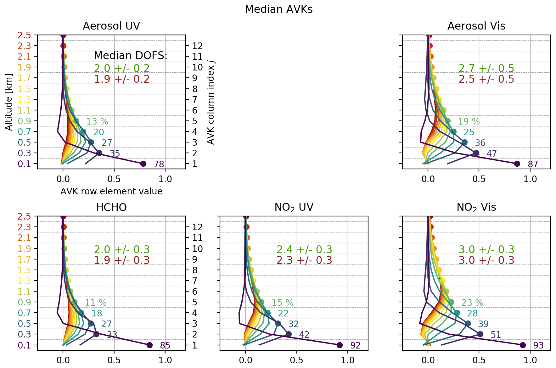
Figure 2 Mean AVKs for the retrieved species (median over participants, mean over time). Their meaning is described in detail in the text. Each altitude and corresponding AVK line A_i are associated with a colour, which is defined by the colour of the corresponding altitude-axis label. The dots mark the AVK diagonal elements. The numbers next to the dots show the exact value in percent, which corresponds to the amount of retrieved information on the respective layer. In each panel, the numbers indicate the DOFS (median among institutes, average over time) for clear-sky (green) and cloudy conditions (red).

With the a priori profiles and covariances used within this study, the sensitivity is limited to about the lowest 1.5 km of the atmosphere for all species. More information is obtained on the Vis species, as the differential light path increases with wavelength resulting in higher sensitivity. The obtained DOFS values are generally a bit lower as observed in former studies. This is related to the rather small a priori covariance (50 %; see Sect. 2.1.3), which implies a good knowledge on the atmospheric state prior to the retrieval and finally leads to less gain in information from the measurements. Figures S35, S36, S37, S38 and S39 in Supplement Sect. S8.1 show the average AVKs of the individual participants and reveal that there are significant differences (up to 1 DOFS) between the participants even when using the same algorithm (up to 0.5 DOFS in the case of PriAM). This indicates that the information content is not assessed consistently. BOREAS, for instance, states a very low gain in information especially for aerosol Vis. This is related to an additional Tikhonov term used as a smoother which was also applied during AVK assessment. Furthermore, all BOREAS results were retrieved on another grid and interpolated onto the submission grid, which leads to a decrease in all AVKs and therefore the DOFS. On average, the dependence of the total amount of information on the cloud conditions is small (typically decrease of 0.1 DOFS). Examination of the AVKs of individual profiles (not shown here), indicated that there are two competing effects: (1) the presence of clouds can increase the sensitivity to higher layers due to multiple scattering and thus light path enhancement in the clouds, whereas (2) a decrease in the horizontal viewing distance (e.g. due to fog, rain or high aerosol loads) reduces the information content, since the light paths are shorter and their geometry depends less on the viewing elevation.

3.2 Overview plots

Figures 3 to 7 show the retrieved profiles of all participants over the whole semi-blind period. They serve as the basis for a general qualitative comparison. For the trace gases, the altitude ranges (full range is 4 km) were reduced to 0–2.5 km for better visibility, considering the MAX-DOAS sensitivity range and the occurrence altitude of the respective species.

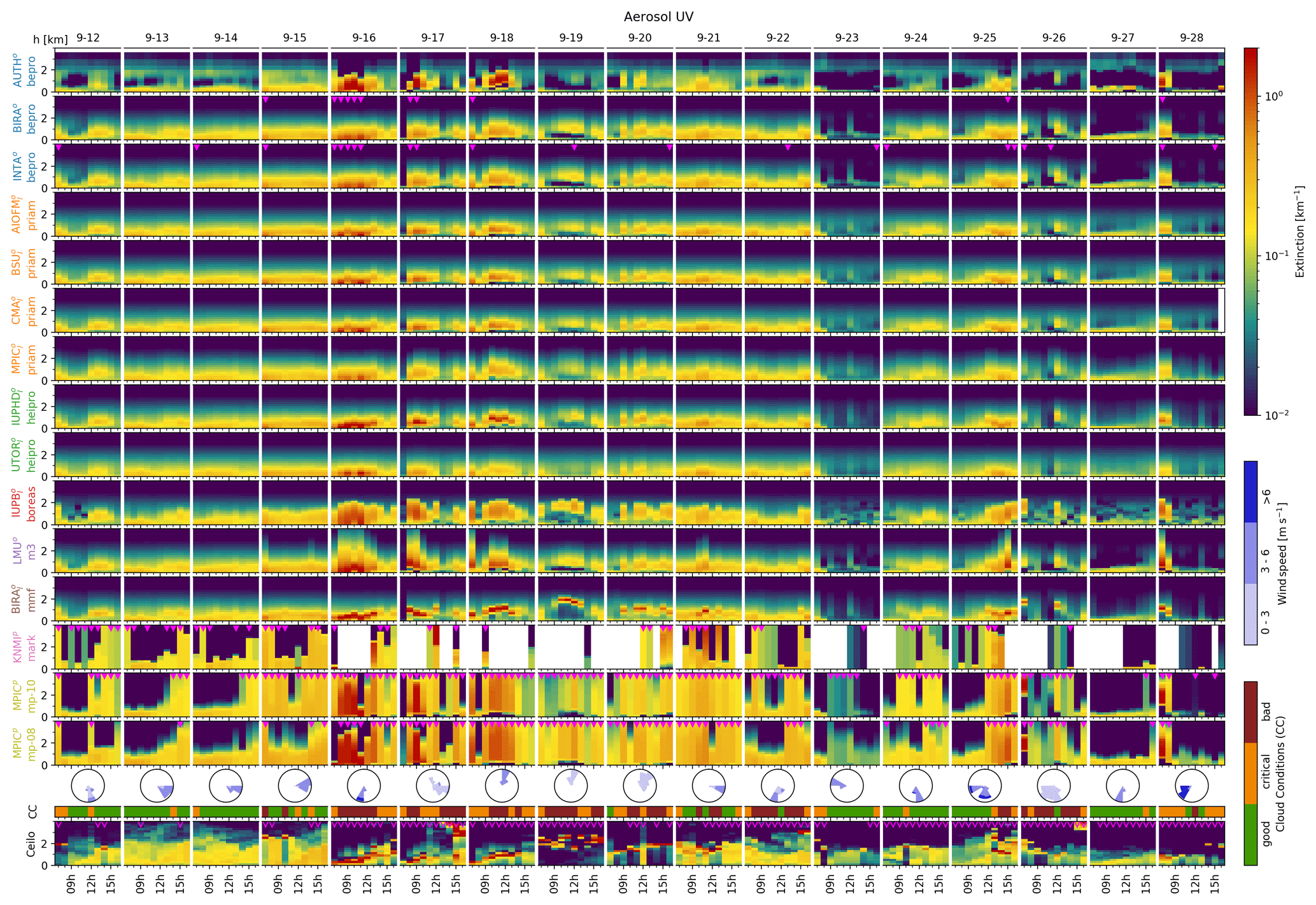
Figure 3 Aerosol UV extinction profiles. For MAX-DOAS profiles (plots above the wind roses), pink triangles at the top of the corresponding profile indicate invalid data. The lowest row shows AOT scaled ceilometer backscatter profiles, calculated as described in Sect. 2.2.2 (unsmoothed). Backscatter profiles, which were scaled from MAX-DOAS AOTs (and which are therefore not fully independent) are marked by pink triangles. Maximum extinction values reach 20 km⁻¹, exceeding the colour scale. Index letters behind the participant labels indicate whether an OEM (o) or parameterized (p) approach was used and whether aerosol was retrieved in the logarithmic space (l). The wind roses in the lower part of the panel show wind direction (azimuth), wind speed (see colour bar on the right) and occurrences (amplitude). The line close to the panel bottom marked with “CC” indicates the cloud conditions, as described in Sect. 2.2.6.

Figure 4 Aerosol Vis extinction profiles. Caption of Fig. 3 applies.

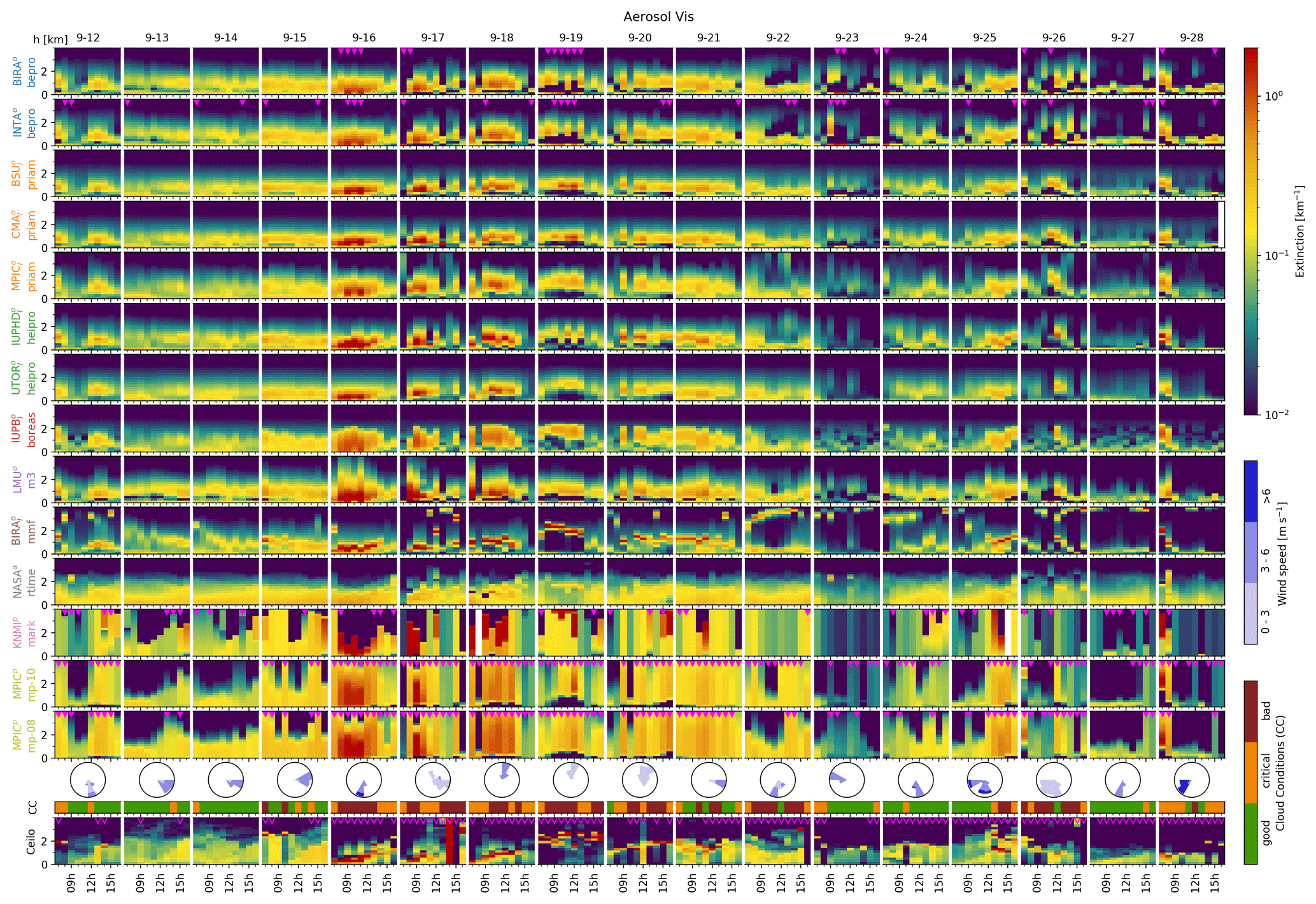
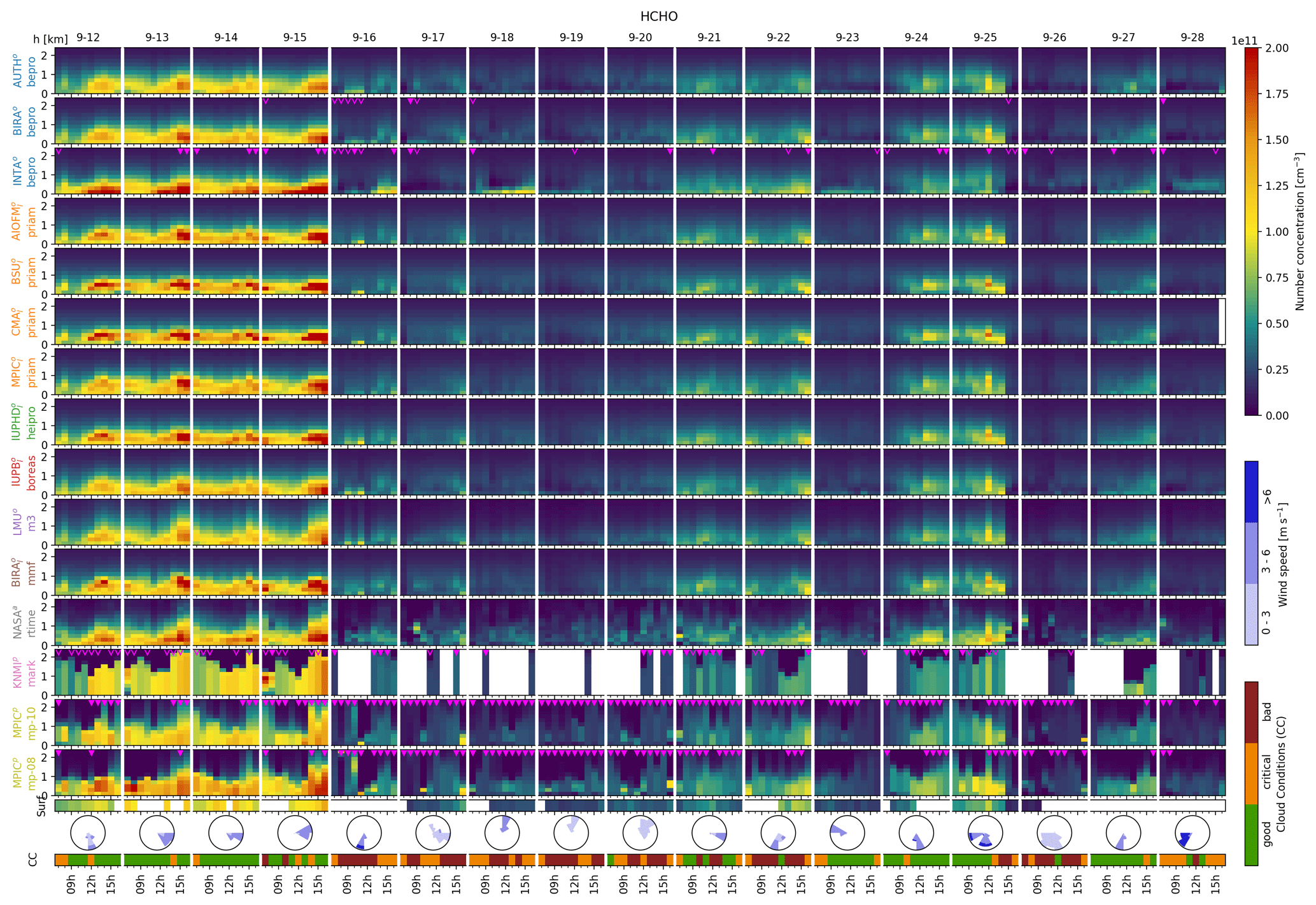
Figure 5 HCHO concentration profiles. The plot is similar to that in Fig. 3. Open pink triangles at the top of the MAX-DOAS profiles indicate that the underlying aerosol retrieval failed, whereas the trace gas profile retrieval itself was considered successful. The “surf” row shows LP-DOAS surface concentrations.

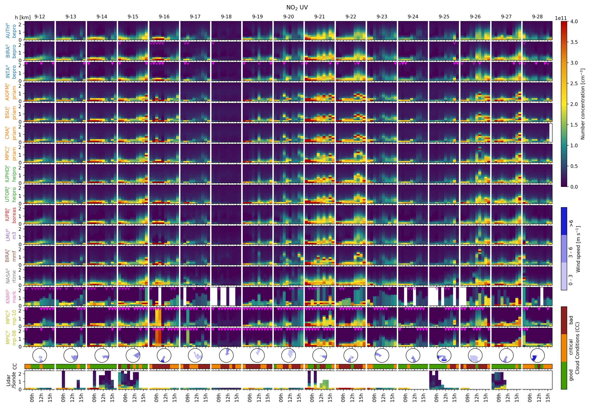
Figure 6 NO₂ UV concentration profiles. The lowest row shows a combined dataset of NO₂ lidar, radiosonde, LP-DOAS and tower in situ data. Redundant surface concentration measurements were averaged.

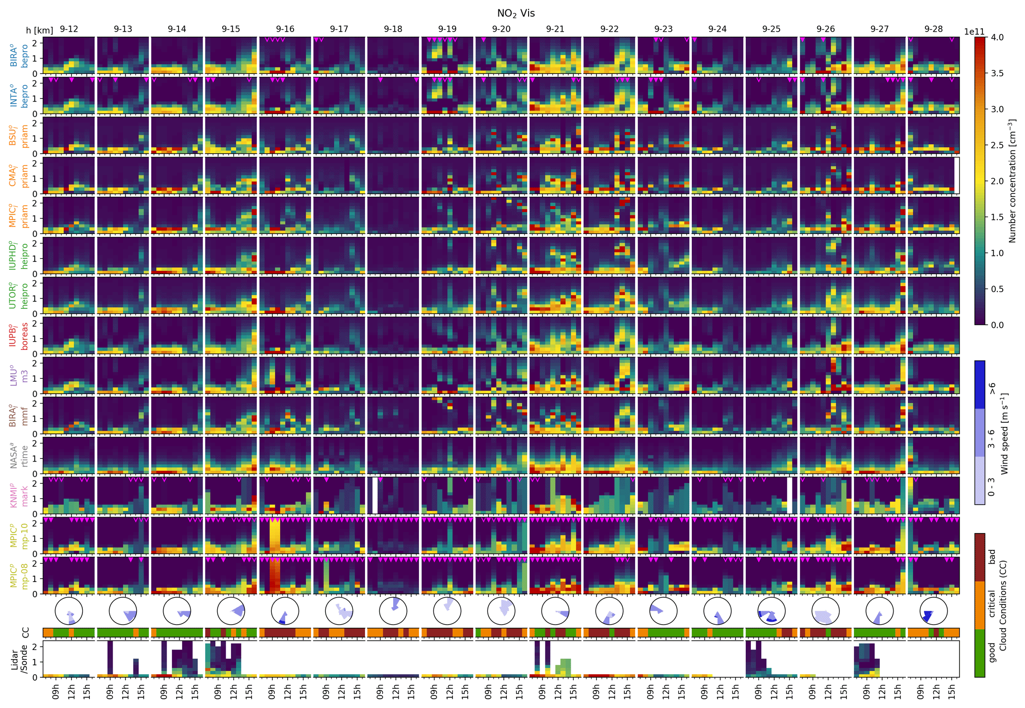
Figure 7 NO₂ Vis concentration profiles. The lowest row shows a combined dataset of NO₂ lidar, radiosonde, LP-DOAS and tower in situ data. Redundant measurements were averaged here.

Considering valid data only, all algorithms detect similar features in the vertical profiles but smoothed to different amounts and sometimes detected at different altitudes. For clear-sky conditions, the observed ASDevs are $\mathrm{3.5}\times {\mathrm{10}}^{-\mathrm{2}}{\mathrm{km}}^{-\mathrm{1}}$ for aerosol UV, $\mathrm{4.0}\times {\mathrm{10}}^{-\mathrm{2}}{\mathrm{km}}^{-\mathrm{1}}$ for aerosol Vis, $\mathrm{1.2}\times {\mathrm{10}}^{\mathrm{10}}\mathrm{molec}.{\mathrm{cm}}^{-\mathrm{3}}$ for HCHO, $\mathrm{2.4}\times {\mathrm{10}}^{\mathrm{10}}\mathrm{molec}.{\mathrm{cm}}^{-\mathrm{3}}$ for NO₂ UV and $\mathrm{4.4}\times {\mathrm{10}}^{\mathrm{10}}\mathrm{molec}.{\mathrm{cm}}^{-\mathrm{3}}$ NO₂ Vis. When regarding participants using the same algorithm, these values are reduced only by about 50 %, indicating that significant discrepancies are caused by differences in the user-defined retrieval settings that were not prescribed. The latter are, for instance, the accuracy criteria for the RTMs, the number of iterations in the inversion, the convergence criteria or the decision at which points of the iteration process the forward model Jacobians are (re)calculated. An example are the discrepancies between UTOR/HEIPRO and IUPHD/HEIPRO. In this case, the number of applied iteration steps in the aerosol inversion was identified as the main reason: UTOR and IUPHD used 5 and 20 iterations here, respectively. The consequences are evident throughout the comparison. Another example is the aerosol UV retrieval of AUTH/bePro, where in contrast to other bePRO users oscillations seem to appear. We suspect this to originate for similar reasons, which could not yet be identified.

In general, larger discrepancies appear for the species measured in the Vis spectral range than in the UV. For NO₂ (aerosol), the ASDev increases in the Vis by 50 % (90 %). In the case of OEM algorithms, a reason might be that there is lower information content in the UV, meaning that the retrievals are drawn closer to the collectively used a priori profile. Further, the larger viewing distance of the Vis retrievals (see Supplement Sect. S5) might be problematic, since the exact treatment of the viewing geometries (like the Earth's curvature or the treatment of the instrument field of view) gains influence. Note that the worsened performance in the Vis was also apparent in the study by Frieß et al. (2019) with synthetic data. The presence of clouds affects ASDevs very differently for different species: for aerosol UV and Vis, it is degraded by factors of 3 and 4, respectively, which is expected since clouds mostly feature high optical depths > 1 and are detected to very different extent by the individual participants. For HCHO, the ASDev decreases by 38 %, which can be well explained by the systematically lower (−36 %) HCHO concentrations observed under cloudy conditions. ASDevs for NO₂ increase by about 20 %, while the observed concentrations remain similar (increase <10 %).

Considering valid data only, the parameterized approaches are mostly in good agreement with the other algorithms. For MAPA, unrealistic results are reliably identified and flagged as invalid, whereas in the case of MARK some valid profiles do not look plausible, e.g. for aerosol Vis on 22 September 2016. For both algorithms, a large fraction (30 % to 70 %) of the profiles are discarded as invalid or look unrealistic if the retrieval conditions are not ideal (see also flagging statistics in Sect. 4). Gaps in the MARK data appear where no optimum solution could be found at all. For aerosol, OEM algorithms often see elevated layers in the Vis even in clear-sky scenarios that cannot be observed in the UV or the ceilometer profiles. On cloudy days, MMF (see Table 2 for definition) is capable of detecting clouds as very defined features with a good qualitative agreement with the ceilometer data. In the Vis, even high clouds are detected, e.g. on 17 and 22 September 2016, which indeed coincide with high-altitude clouds above the retrieval altitude range of 4 km. In contrast to the PAR approaches, OEM and Realtime algorithms yield realistic profiles also under less favourable measurement conditions (e.g. clouds); in particular, the OEM results are in qualitative agreement with the ceilometer profiles for many cases.

Regarding HCHO, the agreement of the profiles is exceptionally good considering the particularly low information content of the measurements (due to higher uncertainties in the dSCD data). This is probably because observed spatial and temporal concentration gradients are much smaller than for NO₂, which might partly be related to enhanced smoothing by the retrieval but is also very likely to be real, since HCHO sources (mainly the photolysis of volatile organic compounds) are less localized. High HCHO concentrations coincide with clear-sky conditions and wind from the continent, which is what would be expected from the current knowledge on the origin and chemistry of atmospheric HCHO. As in the case of aerosol, there are significant discrepancies among the bePRO participants, this time with INTA standing out of the group with slight overestimation.

For NO₂, very shallow layers and large vertical and horizontal gradients might complicate the retrievals. Nevertheless, good ASDev is achieved in the UV. Weekdays and weekends (17, 18, 24 and 25 September) can clearly be distinguished. The lowest concentrations are observed on 18 September, where a Sunday coincides with northerly winds from the sea.

The agreement with the supporting observations will be discussed in detail in the following sections.

3.3 Modelled and measured dSCDs

An intrinsic indicator for a successful profile retrieval is a good agreement between the measured and the modelled dSCDs, the latter being the dSCDs obtained from the RTM model for the finally retrieved aerosol and trace gas profiles. Poor agreement might indicate that only a local minimum of the cost function was found (OEM approaches) that inappropriate retrieval settings were chosen (e.g. too-low number of iterations in the minimization) or that the RTM is inaccurate for other reasons, for instance, because it cannot describe horizontal inhomogeneities. Figures 8 to 12 show the correlation of measured and modelled dSCDs for all profiles and elevations of each participant. The NASA/Realtime algorithm is not included since it does not use an RTM and therefore does not provide simulated dSCDs.

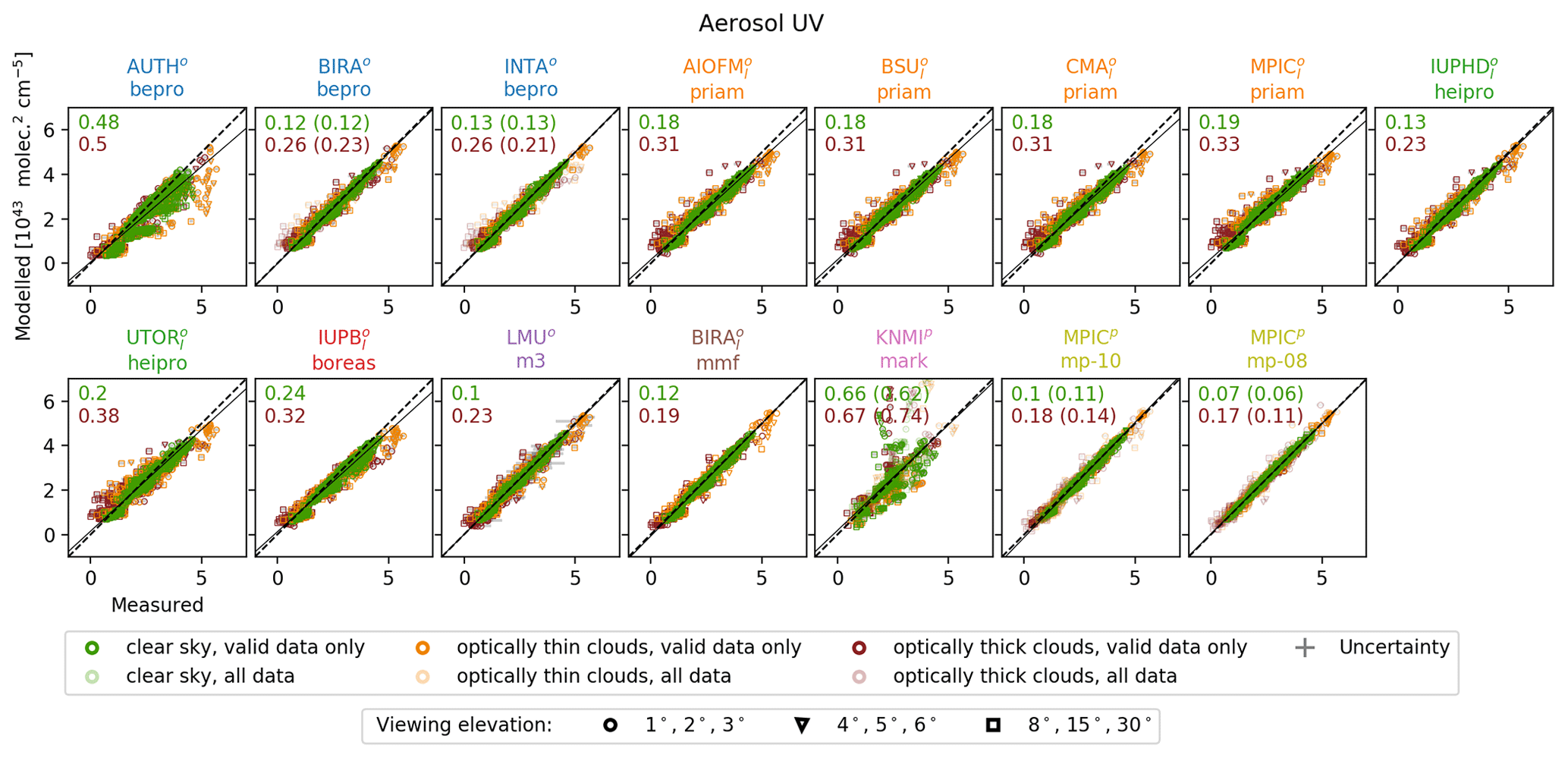
Figure 8 O₄ UV dSCD correlation. Marker colours and marker shapes indicate the cloud conditions and viewing elevation angles, respectively, as indicated in the legend. Numbers represent the measurement-error-weighted RMSD between measured and modelled dSCDs is in units of ${\mathrm{10}}^{\mathrm{43}}\mathrm{molec}{.}^{\mathrm{2}}{\mathrm{cm}}^{-\mathrm{5}}$ for clear-sky (green) and cloudy (red) conditions. Values in brackets were calculated only considering valid data.

Figure 9 O₄ Vis dSCD correlation. Legends and description of Fig. 8 apply.

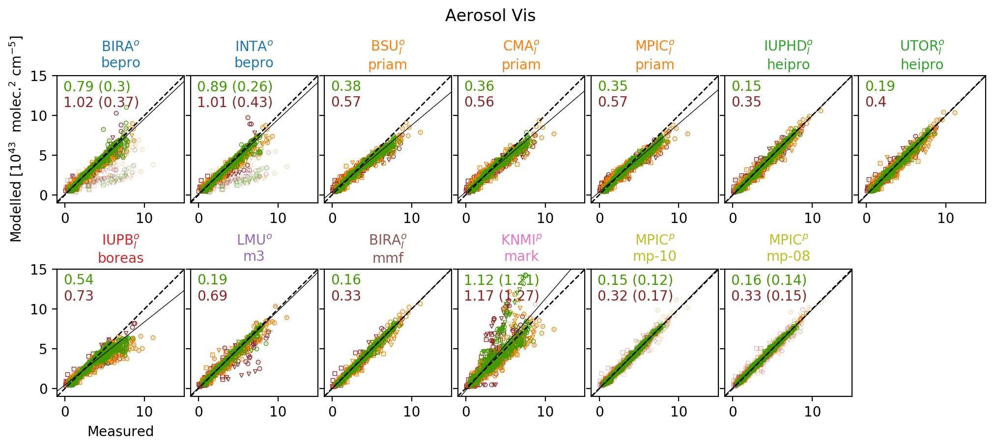
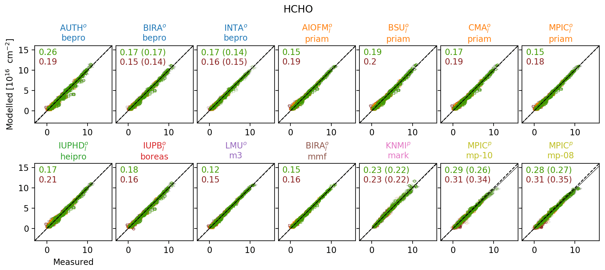
Figure 10 HCHO dSCD correlation. RMSD between measured and modelled dSCDs is in units of ${\mathrm{10}}^{\mathrm{16}}\mathrm{molec}.{\mathrm{cm}}^{-\mathrm{2}}$. Legends and description of Fig. 8 apply.

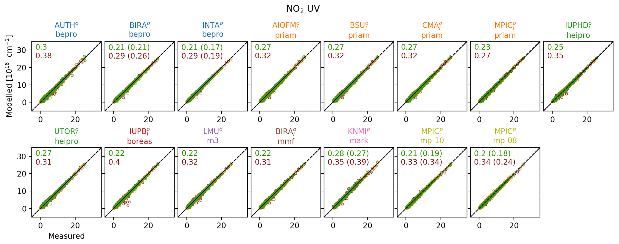
Figure 11 NO₂ UV dSCD correlation. RMSD between measured and modelled dSCDs is in units of ${\mathrm{10}}^{\mathrm{16}}\mathrm{molec}.{\mathrm{cm}}^{-\mathrm{2}}$. Legends and description of Fig. 8 apply.

Figure 12 NO₂ Vis dSCD correlation. RMSD between measured and modelled dSCDs is in units of ${\mathrm{10}}^{\mathrm{16}}\mathrm{molec}.{\mathrm{cm}}^{-\mathrm{2}}$. Legends and description of Fig. 8 apply.

For clear-sky conditions, good agreement is achieved by most participants. Only IUPB/BOREAS, AUTH/bePRO, BSU/PriAM and KNMI/MARK exceed relative RMSDs of 10 % and only for O₄ and NO₂ Vis dSCDs. MMF achieves the best overall performance, being the only algorithm with relative RMSDs <5 % for all species. Regarding HEIPRO, UTOR yields larger RMSD values than IUPHD, which is very likely related to the aforementioned smaller number of iterations applied by UTOR. For the trace gases, small relative RMSD values between 8 % and 8 % are achieved for all cloud conditions.

Regarding aerosol, PriAM and BOREAS feature slightly too-low slopes in the UV (approx. 0.9) and more pronounced in the Vis (0.8 to 0.85), interestingly almost exclusively caused by data recorded on 23 and 27 September where the atmospheric aerosol load is particularly low. RMSDs increase for cloudy scenarios by 10 % (HCHO), 30 % (NO₂ UV) and 50 % (NO₂ Vis, O₄), most likely because the horizontal inhomogeneity cannot be adequately reproduced by the 1-D models. This is supported by the comparison results from synthetic data by Frieß et al. (2019), where horizontal homogeneity is inherently assured and the scatter remains similar for all cloud scenarios. KNMI/MARK has problems reproducing O₄ dSCDs (relative RMSD>30 %), while for trace gases the performance is comparable to the other algorithms. Regarding Vis species, M³ shows outliers under cloudy conditions (while performing excellently in the UV) and bePRO seems to have convergence problems, which was also evident in the synthetic data (Frieß et al., 2019). This problem is overcome by flagging of approx. 10 % of the data, reducing the RMSD by >50 %. PriAM (except MPIC) shows outliers, in particular for NO₂ Vis. The O₄ scaling factor of 0.8 for MAPA improves O₄ dSCD agreement in the UV by about 35 % (for clear-sky and valid data) but not in the Vis spectral range (see also Supplement Sect. S2).

3.4 Aerosol optical thickness

This section compares vertically integrated MAX-DOAS aerosol extinction profiles with the AOTs observed by the nearby Sun photometer. In former publications (e.g. Irie et al., 2008; Clémer et al., 2010; Frieß et al., 2016; Bösch et al., 2018) and also during this comparison study, it was found that MAX-DOAS vertically integrated aerosol profiles systematically underestimate AOTs. It has already been proposed by Irie et al. (2008), Frieß et al. (2016) and Bösch et al. (2018) but not proven that this is related to smoothing effects, namely the reduced sensitivity of MAX-DOAS observations to higher altitudes and associated a priori assumptions. Even though the sensitivity to elevated layers was observed to be increased by the presence of optically thick aerosol layers at the corresponding altitudes (Frieß et al., 2006 and Sect. 3.1 of this study), high-altitude abundances of trace gases and aerosol typically cannot be reliably located and quantified by ground-based MAX-DOAS observations, while aerosol aloft may even introduce systematic errors (Ortega et al., 2016). Integrated profiles rather provide “partial AOTs” which basically only consider low-altitude aerosol and which are additionally biased by a priori assumptions on the aerosol extinctions at higher altitudes (for OEM algorithms defined by the a priori profile and covariance, for PAR algorithms partly in the form of prescribed profile shapes). Therefore, a comparison between MAX-DOAS and Sun photometer is not necessarily meaningful. However, for OEM approaches, information on the true aerosol extinction profile x (which is available from the ceilometer as described in Sect. 2.2.2) and the AVKs A can be used to account for this effect: inserting x and A into Eq. (9) yields a smoothed profile $\stackrel{\mathrm{̃}}{\mathit{x}}$ that can be used to estimate which fraction f_τ of the aerosol column is expected to be detected by the OEM retrievals:

$$\begin{array}{}\text{(10)}& f_{\mathit{\tau }}={\displaystyle \frac{{\mathit{\tau }}_{\mathrm{s}}^{\prime }}{{\mathit{\tau }}_{\mathrm{s}}}}={\displaystyle \frac{{\sum }_i{\stackrel{\mathrm{̃}}{x}}_i}{{\sum }_j{x}_j}},\end{array}$$

with ${\mathit{\tau }}_{\mathrm{s}}^{\prime }$ being the actually detectable “partial AOT”. The left panel of Fig. 13 shows an example of an extreme case during the campaign from 15 September, 15:00 UT. Shown are a ceilometer backscatter profile (x, black) and the same profile smoothed by the MAX-DOAS median OEM averaging kernels for aerosol UV and aerosol Vis (x_UV and x_Vis, blue and green), respectively. In this particular case, it is expected that a large fraction of the aerosol above 1 km altitude will hardly be detected by the MAX-DOAS instruments, resulting in factors $f_{\mathit{\tau }}=\frac{{\mathit{\tau }}_{\mathrm{s}}^{\prime }}{{\mathit{\tau }}_{\mathrm{s}}}$ of 0.67 and 0.78 for the UV and the Vis AOT, respectively. Note, however, that corresponding information actually seems to be present in the measurements, since part of the high-altitude aerosol appears to be shifted to lower altitudes which are accessible within the constraints of the a priori covariance. Multiplying the AOT observed by the Sun photometer with f_τ significantly improves the agreement between MAX-DOAS and Sun photometer observations in particular in the UV. In the following, this is referred to as the PAC. The right panels in Fig. 13 show information on f_τ and the improvement in the UV and Vis results (second and third columns of the figure) over the whole campaign. Average values are $f_{\mathit{\tau }}=\mathrm{0.81}\pm \mathrm{0.16}$ in the UV and (0.9±0.13) in the Vis (using the median AVKs of all OEM retrievals). It shall be pointed out that for OEM algorithms the necessity for the PAC can generally be reduced by using improved a priori profiles and covariances (e.g. from climatologies, supporting observations and/or model data). Also the values for f_τ will differ, when other a priori profiles and covariances than the ones prescribed for this study (see Sect. 2.1.3) are used.

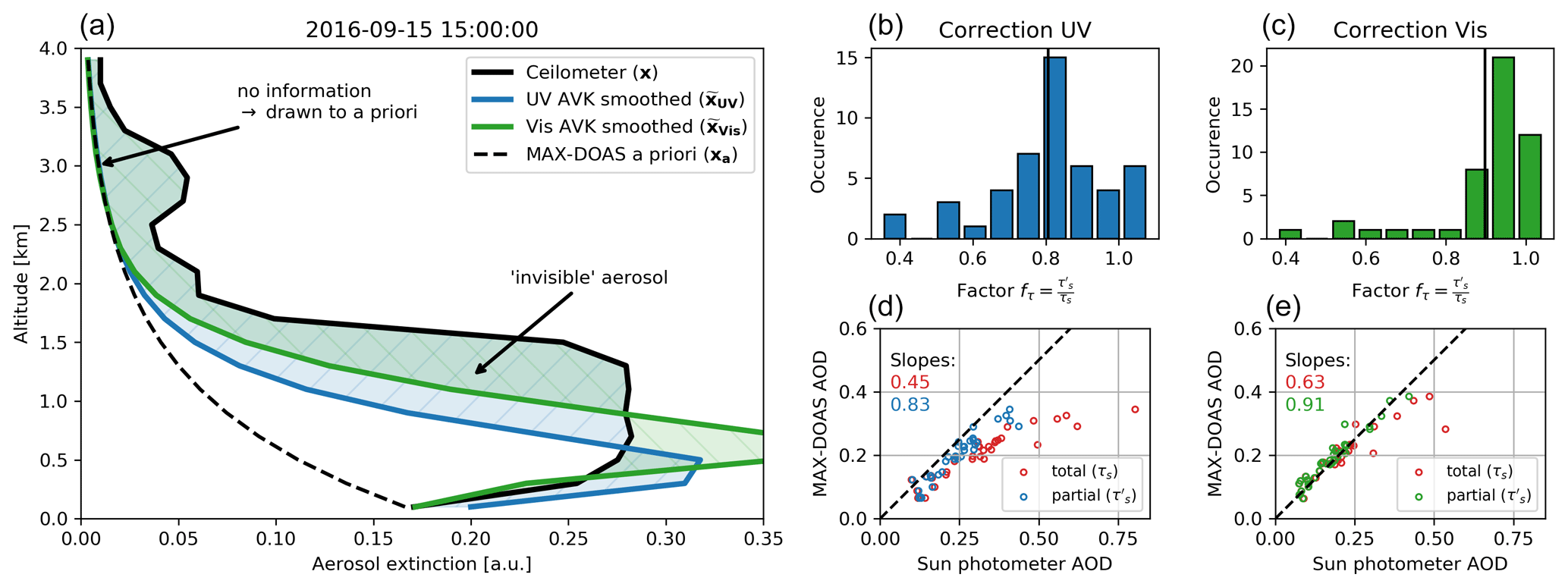
Figure 13 Panel (a) shows an example for the smoothing of a ceilometer backscatter profile x (according to Eq. 9) with particularly heavy aerosol load at high-altitudes retrieved in the UV and Vis, respectively. Panels (b–d) show the distribution and impact of the correction factor $f_{\mathit{\tau }}={\mathit{\tau }}_{\mathrm{s}}^{\prime }/{\mathit{\tau }}_{\mathrm{s}}$ for the UV and the Vis retrieval. Panels (b, c) show the distributions of f_τ with the solid lines indicating the mean values. At the bottom, panels (d, e) show the correlation plots between Sun photometer and MAX-DOAS median AOTs. Red circles represent Sun photometer total AOTs; other dots represent the partial AOT ${\mathit{\tau }}_{\mathrm{s}}=f_{\mathit{\tau }}\cdot {\mathit{\tau }}_{\mathrm{s}}^{\prime }$.

Parameterized and analytical approaches typically do not quantify the sensitivity, the effective resolution or the amount of assimilated a priori knowledge. For these algorithms, the correction could not be performed and the total Sun photometer AOT τ_s had to be used for the comparison in this section. However, the comparison results and further investigations in Supplement Sect. S2 indicate that a scaling of the measured O₄ dSCDs prior to the retrieval with SF≈f_τ might be used to at least partly account for the PAC for MAPA and probably other PAR and ANA algorithms (see Supplement Sect. S2), even though the motivations for the application of the PAC and the SF are different: the application of the PAC is necessary solely for mathematical reasons related to the concept of OEM and prior constraints applied therein. In contrast, publications that suggest or discuss the application of an SF (e.g. Wagner et al., 2009; Clémer et al., 2010, Sect. 2.2; Ortega et al., 2016; Wagner et al., 2019) directly compare forward-modelled O₄ dSCDs (using an atmosphere derived from supporting observations to reproduce the real conditions to the best knowledge) to measured O₄ dSCDs. For the determination of the SF, they do not make use of optimal estimation or prior constraints similar to those used in our study. Thus, their findings can be in general regarded as independent from any kind of PAC, even though PAC and SF have a similar impact on the MAX-DOAS AOT results with the a priori assumptions applied in this study. Particularly, it shall be pointed out that our findings regarding the PAC have no implications on whether elevated aerosol layers explain the necessity of the SF (as proposed by Ortega et al., 2016) or not.

Figure 14 shows the time series of the MAX-DOAS retrieved AOTs in comparison to their median and the Sun photometer data. For the Sun photometer, both the total AOT τ_s and the partial AOT ${\mathit{\tau }}_{\mathrm{s}}^{\prime }$ are shown. For the calculation of ${\mathit{\tau }}_{\mathrm{s}}^{\prime }$ in Fig. 14, the median AVKs of all OEM participants were used for the smoothing according to Eq. (9). In the correlation analysis (Fig. 15), AVKs of the individual participants and the individual profiles were applied. Keep in mind that the non-OEM approaches (NASA/Realtime, KNMI/MARK and MPIC/MAPA) are correlated against τ_s and are therefore expected to generally achieve worse agreement. For correlations of OEM algorithms against τ_s, please refer to Supplement Sect. S8.3. Correlation parameters, RMSD and bias values were derived as described in Sect. 2.3.

Figure 14 MAX-DOAS retrieved AOTs in comparison to Sun photometer data. Symbol and symbol colours are chosen according to Table 2. Transparent symbols indicate data flagged as invalid. (a) MAX-DOAS median results vs. the available supporting observations, according to the legend below the plot. The “institute scatter” areas show the scattering among the participants in terms of standard deviation with valid data considered only. (b, c) Comparison of the individual participants for the two spectral retrieval ranges. Here, the coloured area is the average retrieval error, as specified by the participants.

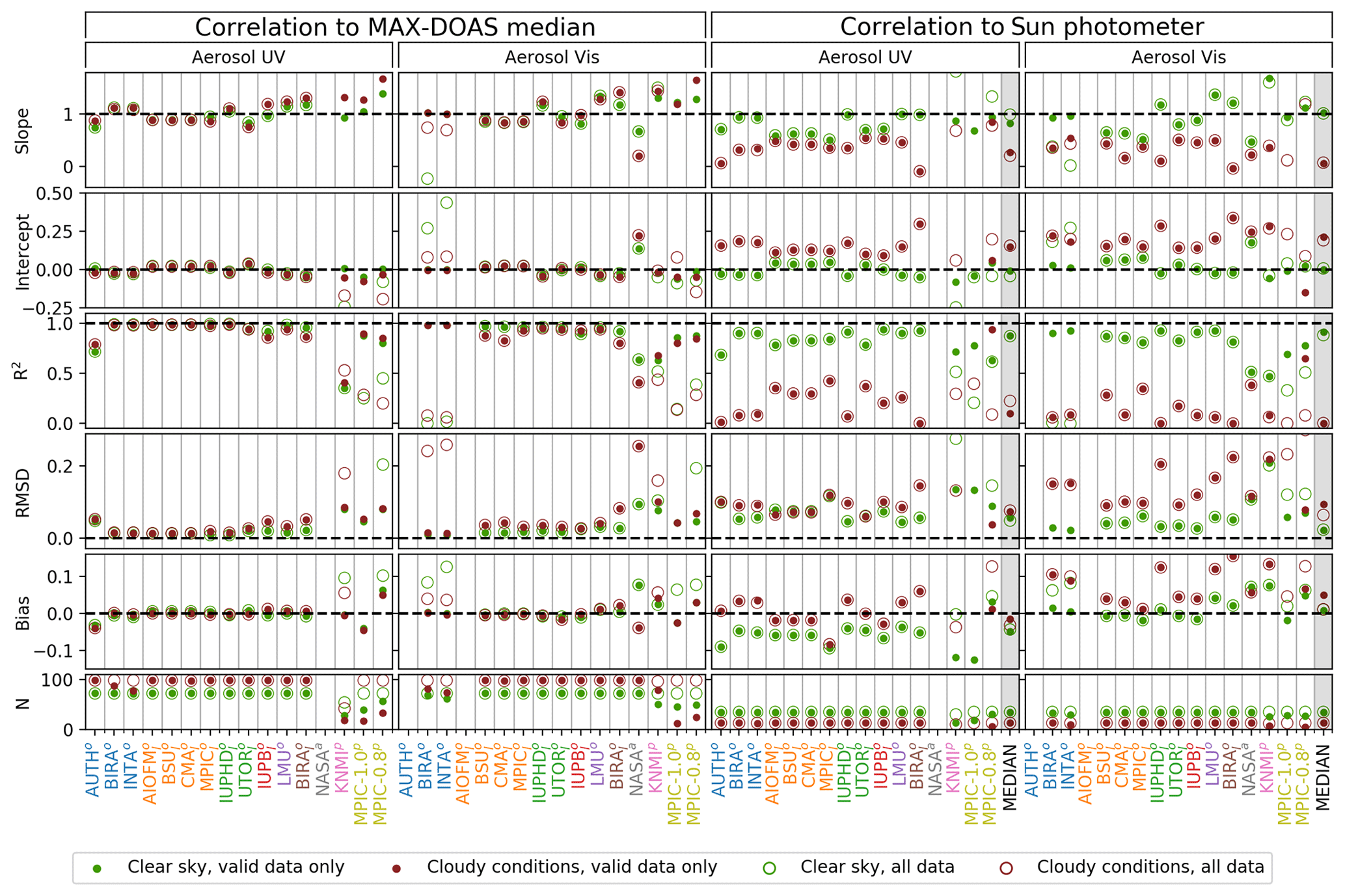
Figure 15 Correlation statistics for AOTs. The two left columns give an impression of the agreement among the institutes, as they show the correlation of the individual participant's retrieved AOT (ordinate of the underlying correlation plot) against the median (abscissa). The two right columns show the correlation against the Sun photometer AOT (partial AOT in the case of OEM retrievals) instead of the median. Green and red symbols represent cloud-free and cloudy conditions, respectively. Hollow circles represent values for all submitted data; the dots only consider data points flagged as valid. N is the number of profiles which contributed to the respective data points above. The total number of submitted profiles per participant and species was 170. On the right, also the correlations between the MAX-DOAS median results and supporting observations are included (grey shaded columns). The correlation plots are shown in Supplement Sect. S8.3.

Under clear-sky conditions, average RMSD values against the MAX-DOAS median are 0.028 in the UV and 0.032 in the Vis. In the presence of clouds, they increase by about 30 % and 80 %, respectively, which is to mainly due to the periods of particularly large scatter between 16 and 19 September 2016. As already shown in Sect. 3.2, different algorithms detect clouds to a very different extent. Especially in the presence of optically thick clouds (AOT > 10), this easily induces discrepancies of several orders of magnitudes. The observed average RMSDs are similar to the specified uncertainties (average is 0.025) that are derived from propagated measurement noise and smoothing effects. Keeping in mind that the retrievals were performed on a common dSCD dataset, this indicates that the choice of the retrieval algorithm and the remaining free settings have a severe impact on the results.

For the comparison to the Sun photometer, it shall be noted that the PAC induces further uncertainties, as it incorporates the extinction profiles derived from the ceilometer and the algorithms' AVKs, both being error prone. Further, the comparison to Sun photometer data under cloudy conditions might not be very meaningful as (1) there are only 13 measurements available in the presence of clouds and (2) it is very likely that these measurements were made by looking through very local cloud holes, such that they will not be representative of the MAX-DOAS retrieved AOTs with a typical horizontal sensitivity range of several kilometres (see Supplement Sect. S5). The following discussion of the Sun photometer comparison therefore refers to clear-sky conditions and valid data only. In general, there is reasonable agreement of the MAX-DOAS retrieved AOT with the Sun photometer, with average observed RMSDs of 0.08 (0.06) for aerosol UV (Vis). Best performance in the UV is observed for IUPHD/HEIPRO and LMU/M³ with RMSDs around 0.05; in the Vis, it is the participants using the bePRO (BIRA and INTA), the HEIPRO (IUPHD and UTOR) and the BOREAS (IUPB) algorithms. For all participants except MPIC-0.8/MAPA, negative biases $<-\mathrm{0.03}$ in the UV remain, even though the PAC has been applied for the OEM algorithms. The average bias in the UV is −0.06, indicating that the systematic underestimation dominates over random deviations here. Note that the slopes and intercepts vary significantly among the participants, however, in an anti-correlated manner, finally resulting in similar bias values.

The average bias in the Vis is only 0.02. Bias magnitudes are much smaller than RMSDs for many participants here, indicating that in these cases Vis AOTs mainly suffer from random discrepancies. BePRO suffers the aforementioned convergence problems during inversion in the Vis (see Sect. 3.3) but the affected results are reliably flagged. KNMI/MARK, NASA/Realtime and MPIC-1.0/MAPA feature the highest RMSDs around 0.1 and strongest biases below -0.1 in the UV. A particular case is KNMI/aerosol Vis with RMSD>0.2, with and without flagging being applied.

As described in Supplement Sect. S2, the PAC and the application of an O₄ dSCD scaling factor of SF≈f_τ have a very similar impact on the AOT correlation. Consequently, the application of SF=0.8 in the case of MPIC-0.8/MAPA significantly improves the agreement to the Sun photometer total AOT in the UV (f_τ≈0.8), whereas in the Vis (f_τ≈0.9) it leads to an overcompensation with a bias of about 0.05.

3.5 Trace gas vertical column densities

This section assesses the consistency of the VCDs for each of the trace gases HCHO and NO₂. Independent observations of VCDs are the direct-sun DOAS observations but also integrated columns of radiosonde and lidar profiles (NO₂ only). Time series comparisons of all observations are shown in Figs. 16 and 17. For the statistical evaluation in Fig. 18, from the supporting observations only direct-sun observations were considered, as they provide the most complete dataset.

As for AOTs, smoothing effects potentially affect the comparability of MAX-DOAS and direct-sun observations. In contrast to aerosol, only scarce (NO₂) or no (HCHO) information on the true profile is available, and a correction similar to the PAC cannot be performed. However, for NO₂, the available radiosonde profiles could be used for an impact estimate. Ignoring one problematic radiosonde profile on 27 September at 07:00 UT (where NO₂ concentration was close to the radiosonde detection limit and thus instrumental offsets became particularly apparent), correction factors of 1.06±0.05 in the UV and 1.03±0.03 in the Vis are obtained, indicating that the MAX-DOAS retrieved tropospheric NO₂ VCD is affected by smoothing effects to only a few percent. This is expected since NO₂ mostly appears close to the ground. Also in Figs. 6 and 7, NO₂ appears to be confined to the lowermost retrieval layers with concentrations dropping to around zero already at altitudes where MAX-DOAS sensitivity is still significant. Profiles from the NO₂ lidar were not used in this investigation as they often suffer from artefacts at higher altitudes. Regarding HCHO, the MAX-DOAS profiling results on some days show large concentrations over the whole altitude range where the information content of the measurements is significant (compare Figs. 2 and 5), indicating that there might be “invisible” HCHO at even higher altitudes. This is supported in Fig. 16, where MAX-DOAS observations tend to yield smaller VCDs than the direct-sun observations in particular in scenarios with high HCHO abundance.

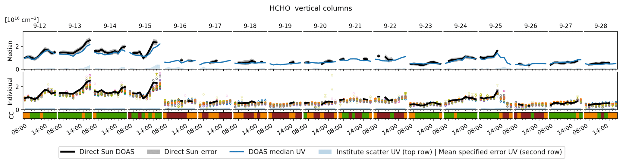
Figure 16 Comparison of MAX-DOAS retrieved HCHO VCDs vs. direct-sun DOAS. Basic descriptions of Fig. 14 apply.

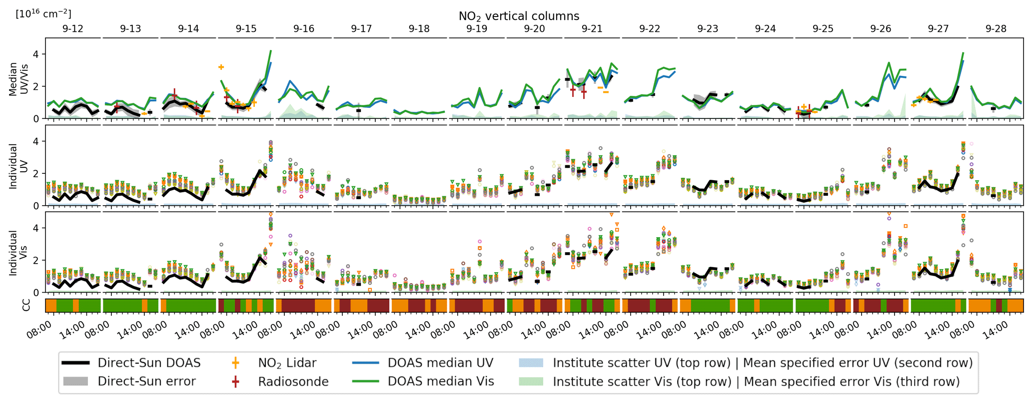
Figure 17 Comparison of MAX-DOAS retrieved NO₂ VCDs vs. direct-sun DOAS, NO₂ lidar and radiosonde. Basic descriptions of Fig. 14 apply.

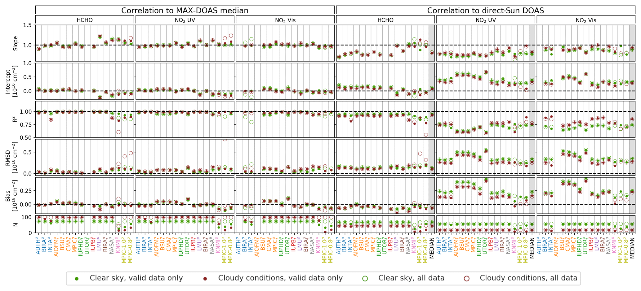
Figure 18 Correlation statistics of trace gas VCDs. The plot is similar to that in Fig. 15. In the underlying correlation plots, ordinates are MAX-DOAS VCDs of individual participants and abscissas are the MAX-DOAS median and direct-sun VCDs, respectively. The correlation plots are shown in Supplement Sect. S8.3.

Under clear-sky conditions, average RMSD values against the MAX-DOAS median are $\mathrm{5}\times {\mathrm{10}}^{\mathrm{14}}\mathrm{molec}.{\mathrm{cm}}^{-\mathrm{2}}$ for HCHO and $\mathrm{7}\times {\mathrm{10}}^{\mathrm{14}}\mathrm{molec}.{\mathrm{cm}}^{-\mathrm{2}}$ for NO₂ (both UV and Vis). In contrast to AOTs, these values do not increase significantly (<15 %) in the presence of clouds. For HCHO, it is even reduced by 25 % for the same reasons as discussed already in Sect. 3.2. Bias values are approximately of half the magnitude of RMSDs for all trace gases.

For HCHO, the comparison against the direct-sun DOAS observations yields an average RMSD of $\mathrm{1.4}\times {\mathrm{10}}^{\mathrm{15}}\mathrm{molec}.{\mathrm{cm}}^{-\mathrm{2}}$. Note, however, that the two observations are not fully independent, as for the direct-sun data, the residual HCHO amount in the reference spectrum was adapted from the MAX-DOAS VCD (see Sect. 2.2.4). Bias values are of the order of 35 % of the RMSDs, indicating that the deviations are mostly random.

For NO₂ UV (Vis), the comparison to the direct-sun DOAS yields an average RMSD of $\mathrm{3.7}\times {\mathrm{10}}^{\mathrm{15}}\mathrm{molec}.{\mathrm{cm}}^{-\mathrm{2}}$ ($\mathrm{3.8}\times {\mathrm{10}}^{\mathrm{15}}\mathrm{molec}.{\mathrm{cm}}^{-\mathrm{2}}$), which is about 5 times the average RMSD of the MAX-DOAS median comparison. Between 12 and 14 September, the direct-sun VCDs but also most radiosonde and lidar observation are systematically lower than the MAX-DOAS VCDs. This is also reflected in the correlation statistics: RMSDs and bias values of different participants appear strongly correlated in Fig. 18 and bias magnitudes are >70 % of the RMSDs for both UV and Vis. The reason could not yet be identified. Interestingly, this contrasts with findings on the surface concentration in the following section, where discrepancies to the LP-DOAS are dominated by random deviations.

In contrast to the AOTs, the RMSDs against the MAX-DOAS median here are smaller than the specified retrieval errors, which are $\mathrm{1.3}\times {\mathrm{10}}^{\mathrm{15}}\mathrm{molec}.{\mathrm{cm}}^{-\mathrm{2}}$ for HCHO, $\mathrm{1.3}\times {\mathrm{10}}^{\mathrm{15}}\mathrm{molec}.{\mathrm{cm}}^{-\mathrm{2}}$ for NO₂ UV and $\mathrm{1.2}\times {\mathrm{10}}^{\mathrm{15}}\mathrm{molec}.{\mathrm{cm}}^{-\mathrm{2}}$ for NO₂ Vis. On the other hand, NO₂ RMSDs against the direct-sun observations are about 3 times larger. For the less abundant HCHO, the signal-to-noise ratio in the median dSCDs is smaller than for other species, such that the specified uncertainties derived from the dSCD noise are larger and more representative of the actual retrieval accuracy.

3.6 Trace gas surface concentrations

This section compares the number concentration of NO₂ and HCHO observed at the surface. Note that in this paper “surface concentration” refers to the average concentration in the lowest MAX-DOAS retrieval layer extending from 0 to 200 m altitude. Independent observations are the LP-DOAS (NO₂ and HCHO) and the surface values of radiosonde and lidar profiles (NO₂), as well as integrated values of in situ measurements in the tower (described in Sect. 2.2.5). Comparisons of all observations are shown in Figs. 19 and 20. For the statistical evaluation (Fig. 21), only LP-DOAS data were considered since they provide a very accurate, representative and complete dataset (see Sect. 2.2.5). The impact of profile smoothing during the retrieval on the retrieved surface concentration was estimated for NO₂ in Supplement Sect. S9 from available radiosonde and lidar NO₂ profiles and was found to be around $\mathrm{5.5}\times {\mathrm{10}}^{\mathrm{9}}\mathrm{molec}.{\mathrm{cm}}^{-\mathrm{3}}$ ($\mathrm{4}\times {\mathrm{10}}^{\mathrm{9}}\mathrm{molec}.{\mathrm{cm}}^{-\mathrm{3}}$) in the UV (Vis). Typical RMSD values in the comparison with the LP-DOAS are about 1 order of magnitude larger, indicating that the impact of smoothing on the NO₂ surface concentration is negligible in this study.

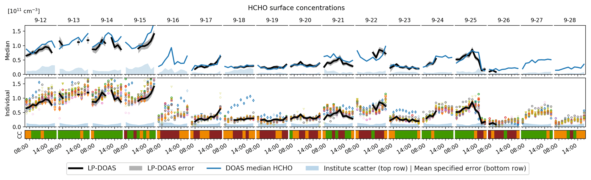
Figure 19 Comparison of MAX-DOAS retrieved HCHO surface concentrations. Basic descriptions of Fig. 14 apply. Note that the mean specified uncertainties in the two lower rows of the figure are very small and thus barely visible.

Figure 20 Comparison of MAX-DOAS retrieved NO₂ surface concentrations. Basic descriptions of Fig. 14 apply. Note that the mean specified uncertainties in the two lower rows of the figure are very small and thus barely visible.

Figure 21 Correlation statistics of trace gas surface concentrations. The plot is similar to that in Fig. 15. In the underlying correlation plots, ordinates are MAX-DOAS surface concentrations of individual participants and abscissas are the MAX-DOAS median and direct-sun VCDs, respectively. The correlation plots are shown in Supplement Sect. S8.3.

The comparisons of surface concentrations are particularly useful, because the largest set of validation data is available here and because in contrast to the comparison of AOT and VCDs, the surface concentration comparison requires an isolation of the surface layer from the layers above and therefore reflects the MAX-DOAS ability to actually resolve vertical profiles at least close to the surface.

Figures 19 and 20 show good qualitative agreement between all observations most of the time, even in the presence of clouds. Apparent exceptions for NO₂ are the fog event on 16 September (strong scatter among the participants) and at forenoon on 22 September (MAX-DOAS median shows large deviations compared to the tower measurements probably due to a very local NO₂ emission event close to the tower).

Under clear-sky conditions average RMSDs observed for the comparison to the MAX-DOAS median results are $\mathrm{8.8}\times {\mathrm{10}}^{\mathrm{9}}\mathrm{molec}.{\mathrm{cm}}^{-\mathrm{3}}$ for HCHO, $\mathrm{1.8}\times {\mathrm{10}}^{\mathrm{10}}\mathrm{molec}.{\mathrm{cm}}^{-\mathrm{3}}$ for NO₂ UV and $\mathrm{2.7}\times {\mathrm{10}}^{\mathrm{10}}\mathrm{molec}.{\mathrm{cm}}^{-\mathrm{3}}$ for NO₂ Vis. For the comparison to the LP-DOAS, these values increase to $\mathrm{1.8}\times {\mathrm{10}}^{\mathrm{10}}\mathrm{molec}.{\mathrm{cm}}^{-\mathrm{3}}$, $\mathrm{4.7}\times {\mathrm{10}}^{\mathrm{10}}\mathrm{molec}.{\mathrm{cm}}^{-\mathrm{3}}$ and $\mathrm{5.6}\times {\mathrm{10}}^{\mathrm{10}}\mathrm{molec}.{\mathrm{cm}}^{-\mathrm{3}}$, respectively. For the median comparison, bias magnitudes are about 40 % of the RMSD values. In contrast to the VCDs, deviations to the supporting observations (LP-DOAS) seem to be random to a large part, as bias magnitudes are about 3 times smaller than RMSDs. Significant biases are only observed for some participants, e.g. UTOR/HEIPRO in the UV.

Clouds have very different impacts on the results: the average RMSD to the median increases by 15 % for HCHO, 26 % for NO₂ UV and 38 % for NO₂ Vis, whereas the average RMSD to the LP-DOAS is even reduced by 4 %, 15 % and 17 %, respectively. A large fraction of the scatter in the comparison to the LP-DOAS might be related to the spatiotemporal variability of the gas concentrations, in particular in the Vis spectral range, where the MAX-DOAS viewing distance is large. The good agreement of the surface concentrations with the supporting observations during the first days is opposite to the VCD comparison, which at least for NO₂ points to a problem with the retrieval results in higher layers or the direct-sun data. For NO₂ Vis, the agreement is generally worse than for NO₂ UV. Convergence problems of bePRO appear again in the form of outliers (see in particular the RMSD values), which are efficiently removed by flagging. INTA shows strong systematic outliers over whole days (e.g. on 18 September), which are not observed for other bePRO users and are very likely produced by technical problems. Again, as for AOTs and VCDs, the scatter among the participants is similar to or larger than the specified errors even for clear-sky conditions (factors of about 1 for HCHO, 2 for NO₂ UV and 3 for NO₂ Vis; see Figs. 19 and 20).

3.7 Retrieval from dSCDs of individual participants

As described in Sect. 2.1.1, the results compared so far were retrieved from a common set of median dSCDs. Thus, the results only illustrate the performance of the different retrieval techniques. However, it is also interesting to compare colocated MAX-DOAS measurements which are fully independent to obtain an estimate of the reliability of a typical MAX-DOAS profile measurement undergoing the whole spectra acquisition and data processing chain. Therefore, the study above was once more conducted with each participant using their own measured dSCDs (see Kreher et al., 2019, for dataset details). Supplement Sect. S10 shows further details by means of figures that are equivalent to those shown before in the course of the median dSCD comparison. A summary is given in Table 5, which shows the increase in the average RMSD and average bias magnitude for the most important comparisons (as described in the preceding subsections for the median dSCDs) when participants use their own instead of the median dSCDs. Only valid data of participants appearing in both studies were considered, and BIRA/bePRO and KNMI were excluded because in contrast to the median dSCD study BIRA/bePRO and KNMI did not submit flags for the own dSCD study, which heavily impacted the results.

Table 5 Relative increase in the average RMSD (first value) and average bias magnitude (values in brackets) when participants retrieve profiles from their own dSCDs instead of using the median dSCDs. Values are given for clear-sky and cloudy conditions separately. Further, the comparisons among the participants (to the MAX-DOAS median) and the comparisons to the supporting observations (Sun photometer AOTs, direct-sun DOAS VCDs and LP-DOAS surface concentrations) are distinguished.

Regarding only the increase in RMSD in the MAX-DOAS median comparison (hence the degradation of consistency among the participants) is qualitatively consistent with what one would expect from the findings by Kreher et al. (2019) on the CINDI-2 dSCD consistency: for NO₂, almost all participating instruments were able to deliver good-quality dSCDs suitable for profile inversion, while for HCHO the quality was much more variable, resulting in the stronger degradation given in Table 5. Kreher et al. (2019) identified instrumental characterization (e.g. detector non-linearity and stray light in the spectrometer) and pointing issues as the main sources of discrepancy between the participant's own dSCD datasets. The degradation is smaller for the surface concentrations than for the trace gas VCDs and is very similar for different cloud conditions.

For the comparison to the supporting observations, the increase in the average RMSD is smaller (second and fourth columns of Table 5). This means that even though using their own dSCDs induces differences among the participants, the average quality of the dSCDs is basically maintained or at least small compared to the discrepancies induced by the retrieval techniques. Interestingly, the RMSD and bias values for the UV AOT and NO₂ VCD even decrease, indicating that the median dSCDs suffer from systematic errors. Under clear-sky conditions, low impact (≤10 %) was found for aerosol UV AOTs and NO₂ data products. Particularly large impact is observed for HCHO VCDs (66 %). Under cloudy conditions, the impact on NO₂ products remains small (again <10 %), whereas for all other products, the increase in the average RMSD exceeds 20 %.

It is also of interest to explicitly estimate which fractions of the total observed discrepancies among MAX-DOAS observations are caused either by the use of different retrieval algorithms or by inconsistencies in the dSCD acquisition. Note that the RMSD values from the median dSCD comparison represent the error arising solely from using different algorithms, while the RMSD values from the own dSCD comparison represent the combined effect of both aspects. For simplicity, we assume that the contributions of both aspects are random and independent so that the effect of using own dSCDs can be isolated by simple RMSD error calculations. For clear-sky conditions, we find that the differences in the measured dSCDs are responsible for approximately 40 % (for AOTs), 85 % (HCHO VCDs), 70 % (HCHO surface concentrations), 50 % (NO₂ VCDs), 40 % (NO₂ UV surface concentrations) and 20 % (NO₂ Vis surface concentrations) of the total variance observed among the participants. The residual variance can be attributed to the choice and setup of the retrieval algorithm.

4 Conclusions

Within this study, 15 participants used nine different profiling algorithms with three different technical approaches (optimal estimation (OEM), parameterized (PAR) and analytical (ANA) approach) to retrieve aerosol and trace gas (NO₂, HCHO) vertical profiles from a common set of dSCDs which was recorded during the CINDI-2 campaign. The results were compared and validated against colocated supporting observations with the focus on aerosol optical thicknesses (AOTs), trace gas vertical column densities (VCDs) and trace gas surface concentrations. Data from some supporting observations were used for qualitative comparison only (ceilometer, NO₂ radiosondes, NO₂ lidar, NO₂ in situ instruments), while for a statistical assessment AOTs from the Sun photometer, VCDs from direct-sun DOAS observations and surface concentrations from the LP-DOAS were used.

Figure 22 shows an overview of RMSD and bias values for the correlation between measured and modelled dSCDs and the comparisons to supporting observations. General strengths and weaknesses of different algorithms become particularly apparent here. Very good overall performance without the need for validity flagging is achieved by the MMF and the M³ algorithm. Note that the results for aerosol are of very similar quality, even though in contrast to M³, MMF retrieves aerosol in the logarithmic space. For valid data (about 20 % discarded), INTA also shows good overall performance apart from the outliers in the HCHO surface concentration, which are very likely related to technical problems. Very good performance for aerosol is observed for IUPHD/HEIPRO over the full dataset. For NO₂, the best performance is achieved by MAPA. The AOT comparison looks generally worse for parameterized approaches, which is expected since no partial AOT correction can be performed, and thus – with the MAX-DOAS integrated extinction profile and the Sun photometer total AOT – basically two different quantities are compared. Finally, the Realtime algorithm by NASA (being the only ANA algorithm) shall be pointed out: despite its simplified radiative transport and the associated outstanding computational performance, it provides reasonable results for trace gases (RMSD/average RMSD around unity).

Parameterized approaches appear to be less stable in the sense that for less favourable conditions no convergence is achieved or inconsistent results are returned (30 % to 70 % of all profiles). For MAPA, these cases are reliably identified and flagged as invalid such that the remaining results achieve very good RMSD and bias values. In contrast, for MARK, even some profiles considered valid do not look plausible. The instability of parameterized algorithms is likely related to the approach: in reality, a vertical profile can be described by an arbitrarily large set of parameters and the information on those contained in a MAX-DOAS measurement depends on the atmospheric conditions and hence the profiles themselves. For parameterized approaches, the number of retrieved parameters is reduced to the number of typically observed DOFS by describing the profile by a few prescribed (not necessarily orthogonal) parameters. Lack of information in those due to particular atmospheric conditions (also if information is available but only on parameters not covered by the chosen parametrization) leads to an underdetermined problem with ambiguous solution and the inversion fails. For OEM approaches, the information can be dynamically distributed to a larger number of parameters (20 in this study, namely the species abundances in the retrieval layers), while parameters of little or no information are constrained by a priori information. This is why OEM inversions converge under a broader range of atmospheric conditions even when information from the measurement is reduced or shifted between retrieved parameters. On the other hand, this means that OEM algorithms even provide plausibly looking profiles (basically the a priori profile) when little or no information is contained in the measurements. Even though such cases can be identified by examining the AVKs, this makes OEM retrievals prone to misinterpretations particularly by inexperienced users.

Regarding full profiles, the overview plots in Sect. 3.2 and figures in Supplement Sect. S8.2 show a good qualitative agreement between the algorithms for valid data and clear-sky conditions. In most cases, they detect the same features; however, these are sometimes at different altitudes and of different magnitude. Under clear-sky conditions, the RMSDs between individual participants and the MAX-DOAS median results are in the range of 0.01–0.1 for AOTs, (1.5–$\mathrm{15})\times {\mathrm{10}}^{\mathrm{14}}\mathrm{molec}.{\mathrm{cm}}^{-\mathrm{2}}$ for trace gas VCDs and (0.3–$\mathrm{8})\times {\mathrm{10}}^{\mathrm{10}}\mathrm{molec}.{\mathrm{cm}}^{-\mathrm{3}}$ for trace gas surface concentrations. These values compare to approximate average AOTs of 0.3, trace gas VCDs of $\mathrm{90}\times {\mathrm{10}}^{\mathrm{14}}\mathrm{molec}.{\mathrm{cm}}^{-\mathrm{2}}$ and trace gas surface concentrations of $\mathrm{11}\times {\mathrm{10}}^{\mathrm{10}}\mathrm{molec}.{\mathrm{cm}}^{-\mathrm{3}}$ observed over the campaign period. Note that profiles were retrieved from a common set of dSCDs, and thus these discrepancies solely arise from the choice of the retrieval algorithm and detailed settings that were not prescribed according to Sect. 2.1.3. An obvious source of discrepancies is the use of different techniques (OEM, PAR and ANA). Further, differences among the two PAR approaches are expected as they use different parameterizations. Note also that the compared algorithms have different priorities: the NASA/Realtime algorithm, for instance, is optimized for computational performance rather than accuracy. Discrepancies among the different OEM algorithms are expected as they retrieve aerosol extinction either in logarithmic or linear space and since the exact implementation might differ (consider, for instance, the Tikhonov regularization approach used by BOREAS). Interestingly, discrepancies among participants using the same OEM algorithm are only about 50 % smaller (regarding ASDevs of profiles as defined in Sect. 2.3) than the average discrepancies among all participants. This indicates that user-defined retrieval settings that were not prescribed within this study (e.g. number of applied iteration steps in the optimization process and RTM accuracy options) also have a significant impact. An example appearing in this study is the differences between IUPHD and UTOR (both using HEIPRO) that were found to mainly be caused by differences in the number of applied iteration steps in the optimization process of the aerosol inversions.

As discussed in more detail below and in Sect. 3.7, the discrepancies among the participants are of a very similar order of magnitude to discrepancies that are induced when participants retrieve profiles from their own measured dSCDs. It is an important finding that, at least for CINDI-2, the choice of the algorithm/settings has a similar impact on the profiling results as the inconsistencies have in the dSCD acquisition.

For the comparison against supporting observations (see Fig. 22), RMSDs increase to a range of 0.02–0.2 against AOTs from the Sun photometer, (11–$\mathrm{55})\times {\mathrm{10}}^{\mathrm{14}}\mathrm{molec}.{\mathrm{cm}}^{-\mathrm{2}}$ against trace gas VCDs from the direct-sun DOAS and (0.8–$\mathrm{9})\times {\mathrm{10}}^{\mathrm{10}}\mathrm{molec}.{\mathrm{cm}}^{-\mathrm{3}}$ against trace gas surface concentrations from the LP-DOAS. For Vis AOTs and trace gas surface concentrations, discrepancies are mostly random (average bias magnitude smaller than half the average RMSD), while for AOT UV and trace gas VCDs systematic deviations are dominant (compare Fig. 22). The average uncertainties of the supporting observations themselves are 0.022, 19×10¹⁴ and $\mathrm{0.74}\times {\mathrm{10}}^{\mathrm{10}}\mathrm{molec}.{\mathrm{cm}}^{-\mathrm{3}}$, respectively, and can therefore be regarded as major RMSD contributors at least in cases where RMSD values are low. Errors in the median dSCDs used as the input for the retrievals are also likely to significantly contribute (see discussion on the dSCD comparison below). Further, investigations on the spatiotemporal variability (see Sect. 2.3.3 and Supplement Sect. S6) indicate that a significant fraction of the RMSD observed between MAX-DOAS and supporting observations is caused by imperfect spatiotemporal overlap. For NO₂, surface concentrations the RMSD resulting from this could roughly be estimated to be around $\mathrm{3}\times {\mathrm{10}}^{\mathrm{10}}\mathrm{molec}.{\mathrm{cm}}^{-\mathrm{3}}$ (using strong simplifications though), which is indeed of the order of magnitude of the average RMSDs observed. Finally, simplified assumptions on the fixed RTM atmosphere were made (compare Sect. 2.1.3). While the choice of pressure and temperature profiles has little impact on the overall agreement with supporting observations (<5 %; see Supplement Sect. S7), the assumptions on the aerosol optical properties (Henyey–Greenstein approximation with constant single scattering albedo and asymmetry parameter over the whole campaign) are a likely source of error.

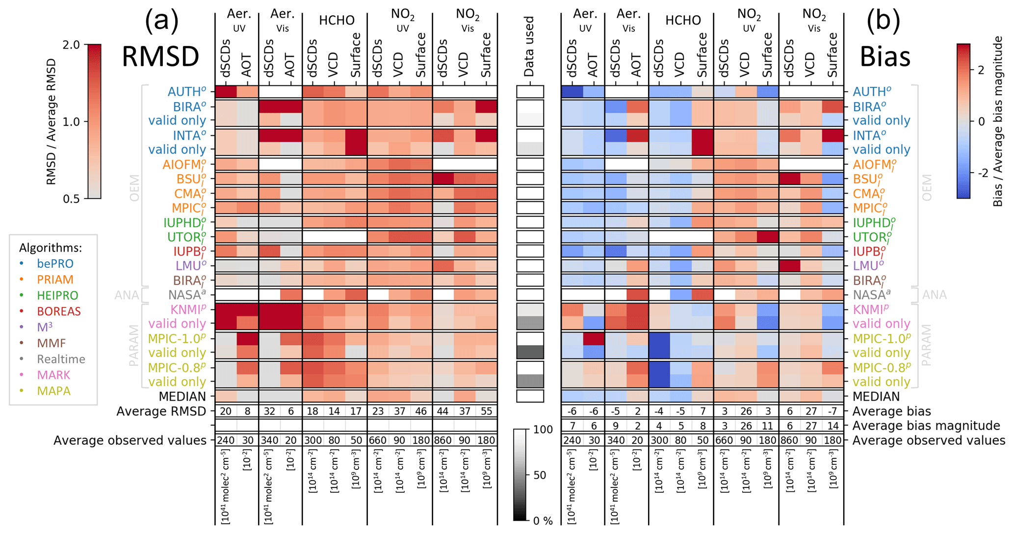
Figure 22 Summary of the comparisons in Sect. 3 for clear-sky conditions: (a) RMSD, (b) bias. Average values of RMSD (bias) define the colour scale of each column of the left (right) panel as indicated by the colour bars on the top left (top right) of the figure. Values of AOT, VCD and surface concentration are given with respect to the corresponding supporting observations (Sun photometer, direct-sun DOAS and LP-DOAS). White spaces indicate no data. Average observed values (bottom row) are rounded campaign averages of the supporting observations. Average bias and average bias magnitude values (third last and second last rows of right panel) represent the averages over the signed and the absolute bias values, respectively. The “data used” column in the centre indicates which fraction of the maximum number (170) of available profiles has been used. Participants who submitted flags are represented by two rows: one considering all data and one using only those flagged as valid (“valid only”).

The consistency of aerosol Vis and NO₂ Vis products (in particular the agreement among the participants) is typically worse in comparison to their UV counterparts by up to several tens of percent. Only the agreement with the Sun photometer AOT improves when going from the UV to the Vis spectral range. This might also be related to the reliability of the Sun photometer AOTs τ_s: while in the Vis the MAX-DOAS retrieval wavelength (477 nm) is close to the lowest Sun photometer wavelength channel (440 nm), in the UV extrapolation of τ_s down to 360 nm is required (see Sect. 2.2.1).

The presence of clouds strongly affects the agreement of aerosol retrieval results particularly in the visible spectral range. For AOTs, the increase in the average RMSD against the median is around 30 % in the UV and 80 % in the Vis, while RMSDs against the Sun photometer are degraded by 10 % and 130 %, respectively. This is expected as (i) high aerosol optical thicknesses at altitudes of low MAX-DOAS sensitivity make the results extremely susceptible to even small changes in the retrieval strategy and (ii) the few Sun photometer observations under cloudy conditions are likely recorded through local cloud holes and therefore not representative of MAX-DOAS measurements integrating horizontally over several kilometres. In contrast, the impact of clouds on average RMSDs for trace gas VCDs is <15 %. Surface concentration RMSDs against the median are degraded by around 25 %, whereas average RMSDs to supporting observations even decrease.

It could be shown that, in the case of CINDI-2, the average impact of smoothing effects on the NO₂ surface concentration is negligible (Supplement Sect. S9). In contrast to that, smoothing has a strong impact on the agreement of MAX-DOAS observations with AOTs and probably HCHO VCDs from supporting observations (Sect. 2.3.2). In particular, it was shown for the first time that formerly observed systematic discrepancies between MAX-DOAS integrated aerosol profiles and Sun photometer AOTs can be largely explained and compensated by considering biases arising from the reduced sensitivity of MAX-DOAS observations to higher altitudes and associated a priori assumptions (see Sect. 3.4).

For CINDI-2 data, there is no clear indication that an O₄ dSCD scaling is necessary. On the one hand, for OEM algorithms, the MAX-DOAS AOT is in good agreement with the Sun photometer partial AOT, and in contrast to Beirle et al. (2019), we find that a scaling factor of 0.8 is too small (Supplement Sect. S2) at least when applied to the whole campaign. On the other hand, a less extreme scaling ($\mathrm{0.8}<\mathrm{SF}<\mathrm{1.0}$) potentially removes remaining biases (see Fig. S3) and improves the agreement between forward model and reality (see Fig. S4). With the a priori settings applied in this study, O₄ scaling and PAC were found to have a similar impact on the MAX-DOAS AOT results. Scaling might therefore be used to at least partly replace the PAC in the case of retrieval approaches that do not quantify their sensitivity or the assimilated a priori information. At last, we think for this study the prescribed scaling factor of 1.0 is justified. Even though it might not be ideal, it is the most straightforward approach and yields reasonable and consistent results within the uncertainties introduced by other factors. To draw more concise conclusions, further studies as performed, e.g. by Wagner et al. (2019) and Ortega et al. (2016) are necessary.

In most comparisons, RMSDs of individual participants against the MAX-DOAS median results (even when using the same algorithm) were of the order of or larger than the uncertainties specified by the algorithms themselves (up to a factor of 3 for NO₂ Vis surface concentrations), indicating that the choice of the retrieval algorithm has a severe impact on the results. It shows further that the specified uncertainties (which typically take propagated measurement noise and smoothing errors into account but neglect other effects like model errors) are too optimistic as a measure for the MAX-DOAS retrieval accuracy and have to be regarded with care.

If the profiles are retrieved from the participant's individually measured dSCDs instead of using a common median dSCD dataset (see Sect. 3.7), the agreement of MAX-DOAS results with supporting observations (average RMSD) is degraded by very different amounts, depending on species and data product. Low impact (≤10 %) was found for aerosol UV AOTs and NO₂ data products. For aerosol UV AOTs and NO₂ UV VCDs, even improvements were observed, hinting at potential systematic errors in the median dSCDs. A particularly strong degradation was observed for HCHO VCDs (65 %). Further, we estimated what fractions of the observed discrepancies among the MAX-DOAS participants are caused either by the use of different retrieval algorithms or by inconsistencies in the dSCD acquisition. On average, the impact of both aspects is very similar: the effect of using own dSCDs can be estimated to contribute 40 % (for AOTs), 85 % (HCHO VCDs), 70 % (HCHO surface concentrations), 50 % (NO₂ VCDs), 40 % (NO₂ UV surface concentrations) and 20 % (NO₂ Vis surface concentrations) to the total variance introduced by both aspects. The high values for HCHO are expected, since according to Kreher et al. (2019), the acquisition of dSCDs was particularly challenging here and they varied widely among the participants.

We summarize our major findings as follows: besides the quality of the spectral data, the applied inversion strategy has a significant impact on the accuracy of MAX-DOAS retrieval results. Nevertheless, partial AOTs, VCDs and surface concentrations can be retrieved with good accuracy, if the algorithm, settings and quality filters are chosen carefully and ideally by experienced users. For the future, we therefore suggest to put a focus on further harmonization of MAX-DOAS retrievals, in particular with regard to their application by the broader scientific community.

For future campaign and comparison exercises, fixed model parameters (particularly aerosol optical properties) and prior constraints might be improved. Further, we suggest putting an enhanced focus on the coordinated operation of all (not only MAX-DOAS) instruments and incorporating techniques with more appropriate spatial kernels, e.g. limb DOAS measurements from unmanned aerial vehicles, to reduce the spatiotemporal mismatch between different observations.