the Creative Commons Attribution 4.0 License.
the Creative Commons Attribution 4.0 License.
 | 10 Feb 2021
Emission Monitoring Mobile Experiment (EMME): an overview and first results of the St. Petersburg megacity campaign 2019
Maria V. Makarova
Carlos Alberti
Dmitry V. Ionov
Frank Hase
Stefani C. Foka
Thomas Blumenstock
Thorsten Warneke
Yana A. Virolainen
Vladimir S. Kostsov
Matthias Frey
Anatoly V. Poberovskii
Yuri M. Timofeyev
Nina N. Paramonova
Kristina A. Volkova
Nikita A. Zaitsev
Egor Y. Biryukov
Sergey I. Osipov
Boris K. Makarov
Alexander V. Polyakov
Viktor M. Ivakhov
Hamud Kh. Imhasin
Eugene F. Mikhailov
Global climate change is one of the most important scientific, societal and economic contemporary challenges. Fundamental understanding of the major processes driving climate change is the key problem which is to be solved not only on a global but also on a regional scale. The accuracy of regional climate modelling depends on a number of factors. One of these factors is the adequate and comprehensive information on the anthropogenic impact which is highest in industrial regions and areas with dense population – modern megacities. Megacities are not only “heat islands”, but also significant sources of emissions of various substances into the atmosphere, including greenhouse and reactive gases. In 2019, the mobile experiment EMME (Emission Monitoring Mobile Experiment) was conducted within the St. Petersburg agglomeration (Russia) aiming to estimate the emission intensity of greenhouse (CO2, CH4) and reactive (CO, NOx) gases for St. Petersburg, which is the largest northern megacity. St. Petersburg State University (Russia), Karlsruhe Institute of Technology (Germany) and the University of Bremen (Germany) jointly ran this experiment. The core instruments of the campaign were two portable Bruker EM27/SUN Fourier transform infrared (FTIR) spectrometers which were used for ground-based remote sensing measurements of the total column amount of CO2, CH4 and CO at upwind and downwind locations on opposite sides of the city. The NO2 tropospheric column amount was observed along a circular highway around the city by continuous mobile measurements of scattered solar visible radiation with an OceanOptics HR4000 spectrometer using the differential optical absorption spectroscopy (DOAS) technique. Simultaneously, air samples were collected in air bags for subsequent laboratory analysis. The air samples were taken at the locations of FTIR observations at the ground level and also at altitudes of about 100 m when air bags were lifted by a kite (in case of suitable landscape and favourable wind conditions). The entire campaign consisted of 11 mostly cloudless days of measurements in March–April 2019. Planning of measurements for each day included the determination of optimal location for FTIR spectrometers based on weather forecasts, combined with the numerical modelling of the pollution transport in the megacity area. The real-time corrections of the FTIR operation sites were performed depending on the actual evolution of the megacity NOx plume as detected by the mobile DOAS observations. The estimates of the St. Petersburg emission intensities for the considered greenhouse and reactive gases were obtained by coupling a box model and the results of the EMME observational campaign using the mass balance approach. The CO2 emission flux for St. Petersburg as an area source was estimated to be 89 ± 28 , which is 2 times higher than the corresponding value in the EDGAR database. The experiment revealed the CH4 emission flux of 135 ± 68 , which is about 1 order of magnitude greater than the value reported by the official inventories of St. Petersburg emissions (∼ 25 for 2017). At the same time, for the urban territory of St. Petersburg, both the EMME experiment and the official inventories for 2017 give similar results for the CO anthropogenic flux (251 ± 104 vs. 410 ) and for the NOx anthropogenic flux (66 ± 28 vs. 69 ).
- Article
(12314 KB) - Full-text XML
- BibTeX
- EndNote


Global climate change is one of the most important scientific, societal and economic contemporary challenges. Fundamental understanding of the major processes driving climate change is the key problem which is to be solved not only on a global but also on a regional scale (IPCC, 2013; WMO Greenhouse Gas Bulletin, 2018). The accuracy of regional climate modelling depends on a number of factors. One of these factors is the adequate and comprehensive information on the anthropogenic impact which is highest in industrial regions and areas with dense population – modern agglomerations and megacities. Agglomerations and megacities are not only “heat islands”, but also significant sources of emissions of various substances into the atmosphere, including greenhouse and reactive gases (Zinchenko et al., 2002; Wunch et al., 2009; Ammoura et al., 2014; Hase et al., 2015; Turner et al., 2015; Viatte et al., 2017). Estimating emission intensity for industrial areas and cities requires precise measurements of gas composition in the troposphere with a high horizontal resolution on a regional scale. Existing ground-based observational networks, in particular ESRL (ESRL, 2019), ICOS (ICOS, 2020), NDACC (NDACC, 2019) and TCCON (TCCON, 2019), are mainly focused on detecting the background concentrations of greenhouse gases. Most of the observational stations are sparsely distributed and located relatively far from industrial and highly populated areas. EM27/SUN portable Fourier transform infrared (FTIR) spectrometers (Gisi et al., 2012; Frey et al., 2015) are very promising instruments for the detection and quantification of the emissions of greenhouse gases from mesoscale area sources like cities or industrial areas (Hase et al., 2015; Chen et al., 2016). The data provided by these instruments are less affected by the vertical exchange processes than the data obtained from in situ measurements. Also, in contrast to current space-based sensors, the ground-based portable FTIR spectrometer data are essentially unaffected by the aerosol burden transported by the pollution plume.
The quantification of the gas fluxes from the sources located on the earth's surface can be carried out using various methods: “forward” and “inverse” modelling (Maksyutov et al., 2013; Turner et al., 2015), the eddy covariance method (Helfter et al., 2011, 2014a), the mass balance approach (Zimnoch et al., 2010; Strong et al., 2011; Hiller et al., 2014a) and a technique based on radon measurements (Lopez et al., 2015). Depending on the method, the spatial coverage of investigated sources can vary from the local (for example, in the case of eddy covariance) to the mesoscale and the global scale (the assimilation of satellite data in atmospheric models). Each of these approaches has its own set of unique advantages and limitations depending on specific spatial and/or temporal scales. Therefore the efficacy and accuracy of many of these methods remain the subject of scientific debate (Cambaliza et al., 2014; Hiller et al., 2014a). Often, combinations of these methods can yield reduced uncertainty of target parameters; at the same time a combination of different techniques often requires special field campaigns and comprehensive analysis (Hiller et al., 2014a, b).
Recently, several studies were performed with the goal to estimate the emissions of industrial regions and cities by means of ground-based mobile measurements of tropospheric gaseous composition using FTIR and differential optical absorption spectroscopy (DOAS) techniques. Hase et al. (2015) and Zhao et al. (2019) applied portable FTIR spectrometers for detecting greenhouse gas emissions of the major city Berlin. In these studies, five portable EM27/SUN spectrometers were used for the accurate and precise observations of column-averaged abundances of CO2 and CH4 around the major city of Berlin. It has been demonstrated that the CO2 emissions of Berlin can be clearly identified in the observations. Chen et al. (2016) developed and used differential column methodology (downwind–upwind column differences) for the evaluation of CH4 emissions from dairy farms in the Chino area. Vogel et al. (2019) investigated the Paris megacity emissions of CO2 by coupling the COCCON observations and atmospheric transport model framework (CHIMERE-CAMS) simulations. Luther et al. (2019) explored the feasibility of estimating CH4 emissions for individual coal mine ventilation shafts and groups of shafts. They measured column-averaged dry-air mole fractions of methane XCH4 using the Bruker EM27/SUN FTIR spectrometer which was installed on a truck moving through the CH4 plumes in the Upper Silesian Coal Basin, while driving in stop-and-go patterns. De Foy et al. (2007), Mellqvist et al. (2010), Johansson et al. (2014) and Kille et al. (2017) have applied mobile FTIR (Solar Occultation Flux technique) and mobile DOAS techniques to large-scale flux measurements. Babenhauserheide et al. (2020) estimated CO2 emissions from Tokyo using the long-term statistical analysis of XCO2 amounts measured at the Tsukuba TCCON site located near Tokyo.
The motivation of the present study originated from the fact that the number of observational stations for greenhouse gas monitoring in the territory of Russia is very limited, and there are considerable uncertainties of the greenhouse gas flux estimations for the natural and anthropogenic sources in Russia. St. Petersburg is the second largest megacity in Russia, with a population of 5 million, and, in addition, it is the northernmost city in the world with a population of over 1 million people. The goal of the present study was to estimate the emissions of greenhouse (CO2, CH4) and reactive (CO, NOx) gases from St. Petersburg by means of mobile remote sensing techniques and direct in situ measurements. The study was based on the observational campaign EMME-2019 (Emission Monitoring Mobile Experiment) which was performed in March–April 2019 in the territory of the St. Petersburg agglomeration. St. Petersburg State University (Russia), Karlsruhe Institute of Technology (Germany) and the University of Bremen (Germany) jointly ran this experiment in the frame of the international project VERIFY (VERIFY, 2019). The idea and the methodology of EMME were based mainly on the studies by Hase et al. (2015), Ionov and Poberovskii (2015), Chen et al. (2016) and Viatte et al. (2017).
The concept of EMME is based on remote measurements of the total column amount of CO2, CH4 and CO from two mobile platforms located inside and outside the city plume (usually at upwind and downwind locations on opposite sides of the city of St. Petersburg) combined with the mobile circular measurements of the tropospheric column amount of NO2 from the third mobile platform moving in a non-stop mode; the latter measurements are used for the real-time control of the megacity plume evolution. The simplified illustration of the concept is given in Fig. 1. The experiment requires clear-sky conditions since the instruments for remote sensing measure direct and scattered solar radiation. The ancillary measurements include control of the meteorological parameters and sampling of air portions at locations inside and outside the city plume for subsequent laboratory analysis of concentrations of target gases. In order to assess the intensity of gas emissions by St. Petersburg, the mass balance approach is applied to the measurement data. The principal feature of EMME is its integrated character: several different instruments are used, and, additionally, the planning of the field experiment and data processing are performed with the help of numerical modelling of the transport of the megacity pollution plume.
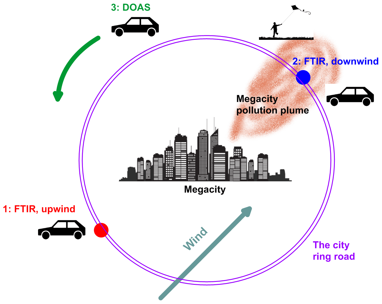
Figure 1Illustration of the concept of EMME: two FTIR spectrometers at the upwind and downwind locations on opposite sides of the city (no. 1 and no. 2, red and blue dots) and circular moving DOAS technique spectrometer (no. 3). Ground-level air samples were collected at locations no. 2 and no. 3. Collecting air portions with the help of a kite was done usually at the downwind location under suitable weather and landscape conditions. Pictogram png images: https://www.cleanpng.com/, last access: 6 November 2019.
The core instruments of the campaign are two portable Bruker EM27/SUN FTIR spectrometers (Gisi et al., 2012; Frey et al., 2015, Hase et al., 2016) which are used for ground-based remote sensing measurements of the total column amount of CO2, CH4 and CO. The EM27/SUN instrument has a sun-tracking system and records direct infrared solar radiation. The FTIR spectrometers are transported by cars to the measurement locations where they are unloaded and installed outside. The geographic coordinates are recorded by the GNSS (Global Navigation Satellite System) sensor. A detached car battery with an inverter is used as a power supply which ensures about 3 h operation time. Under cold weather conditions, the instruments are covered by electric heating blankets. The integration time for a single spectrum constitutes about 1 min. Within this period, about 10 interferograms are recorded and averaged, and then the corresponding spectrum is recorded.
The tropospheric NO2 column is derived from measurements of the scattered solar radiation in the zenith direction by the portable OceanOptics HR4000 automatic spectrometer. This spectrometer is mounted on board a car and connected to a portable computer to ensure uninterruptible recording of spectra. Measurements are fully automatic while the car is moving. The location of the car is controlled by the GNSS sensor and is routinely recorded by the onboard computer for instant referencing of the results of measurements to the car route. The sampling period of time (time of exposure) for a single spectrum is calculated by the software tool accounting for illumination conditions and constitutes about 60 ms on average for the observations at about noon. Recording of spectra is done every 1 min; all single spectra obtained within this period are co-added. Thus, each final measurement is the mean of about 1000 instant spectra. The route includes the entire city ringway (the highway around St. Petersburg); therefore the main emission sources are inside the route, and the position of the megacity plume can be detected with high accuracy. The described approach and the DOAS mobile experiment specific design have been implemented previously in St. Petersburg, and the results have been published by Ionov and Poberovskii (2012, 2015, 2017, 2019).
Air samples were collected at the locations of both FTIR spectrometers in two air bags: when FTIR measurements started (the first bag) and before completion of FTIR measurements (the second bag). Each bag was a 25 L Tedlar bag, sampled for about 40 min. In case of suitable weather and landscape conditions at the location of one of the FTIR spectrometers, sampling bags were lifted by a kite to an altitude of about 100 m. The laboratory analysis of the air samples was performed with the help of gas analysers. A Los Gatos Research GGA 24r-EP gas analyser was used for measuring the volume mixing ratio (vmr) of CH4, CO2 and H2O. A Los Gatos Research CO 23r gas analyser was used for measuring the vmr of CO and H2O. The concentration of NO and NO2 (NOx) was measured by a ThermoScientific 42i-TL gas analyser.
For the monitoring of meteorological parameters, two weather stations and the microwave radiometer RPG-HATPRO were used. One portable weather station was operating either at upwind or at the downwind location of FTIR spectrometers. The atmospheric pressure measurements were performed at both up- and downwind locations. The second stationary weather station was operating on the roof of the building (56 ) of the Institute of Physics of St. Petersburg State University (SPbU), located about 25 km west from the city centre. The RPG-HATPRO radiometer was operating also on the roof of this building and delivered information on the temperature and humidity vertical profiles together with the information on the cloud liquid water path (Kostsov, 2015; Kostsov et al., 2018).
The essential part of EMME was the preparatory stage which lasted for 3 months before the start of the campaign. During this stage the optimal set of FTIR measurement locations in the close vicinity of the St. Petersburg ringway was determined accounting for several criteria. First, this set of locations should have had sufficient spatial density to ensure the possibility to perform up- and downwind FTIR measurements for practically any wind direction. Second, every location should have been convenient for car parking in the ringway proximity and for the installation of the instruments. We tried to choose the locations at a certain distance from the highway and roads with intensive traffic in order to avoid contamination of air by local sources. The set of FTIR measurement locations around the St. Petersburg agglomeration which was chosen during the preparatory stage is shown in Fig. 2. It should be emphasised that during the preparatory stage a kind of rehearsal was carried out. This rehearsal has helped to reveal how time-consuming the following processes are: loading the equipment on cars at the Institute of Physics, unloading the equipment at a measurement location and setting up and tuning the instruments for data acquisition. This information is critical for understanding whether it is possible to reach the desired up- and downwind locations in proper time by different crews and to start simultaneous FTIR measurements.
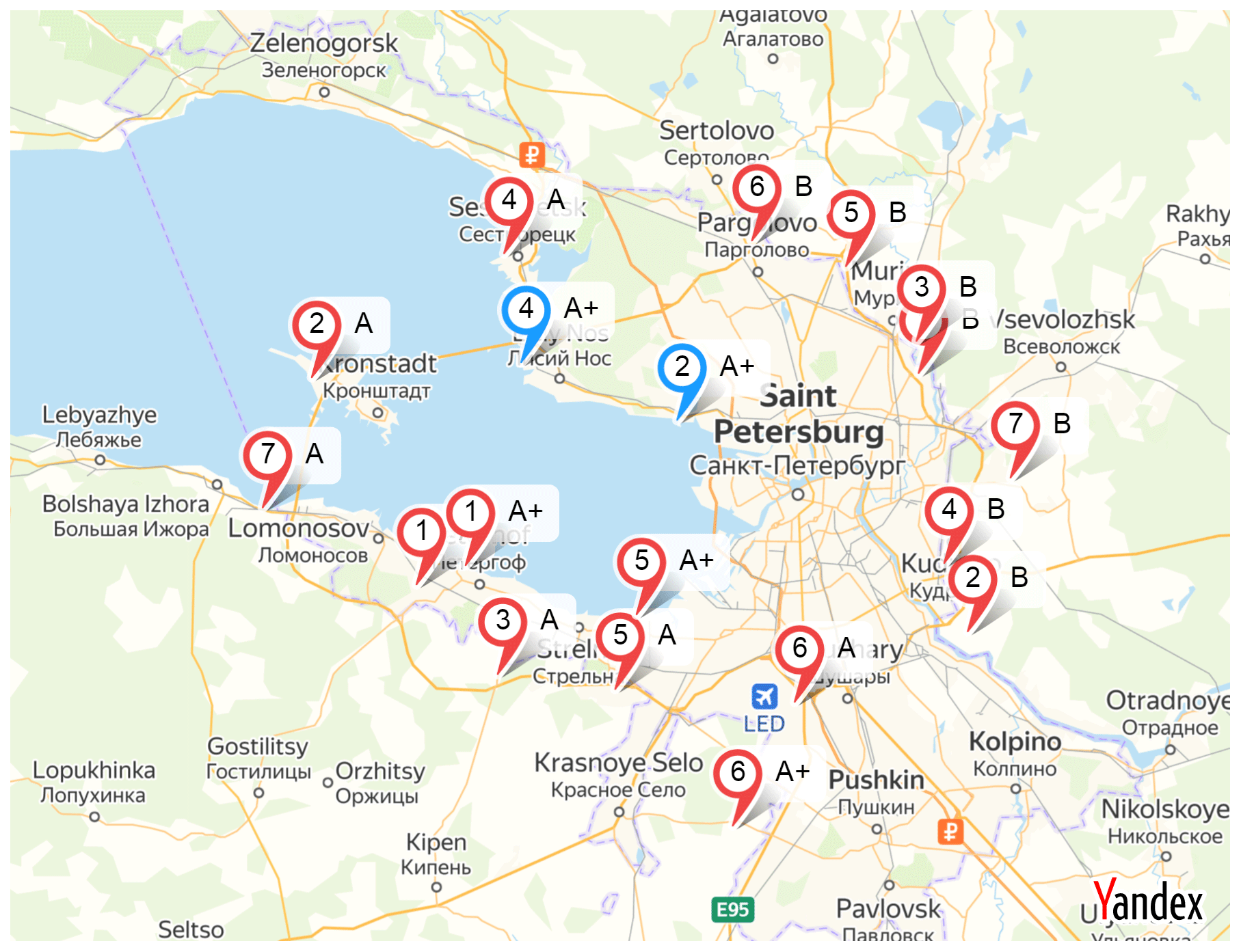
Figure 2The set of FTS locations around the St. Petersburg agglomeration. Locations are marked by letters “A” and “B” with numbers. The “plus” sign near a location mark denotes that there is a possibility to use a local power supply at this location. The red colour denotes primary locations, and the blue colour denotes secondary locations. Map data © 2019 Yandex.
Special attention was paid to the planning of the experiment a day before. We analysed the weather forecasts presented by different sources with special attention to cloud cover and wind direction. Mainly, we used the cloud maps from https://www.msn.com (last access: 12 November 2019). In order to determine FTIR measurement locations for a specific day, we made a forecast of the megacity plume using the HYSPLIT (HYbrid Single-Particle Lagrangian Integrated Trajectories) model (Draxler and Hess, 1998; Stein et al., 2015). In addition, in the morning of a measurement day we monitored the cloud cover using web cameras which operated nearby the planned measurement locations.
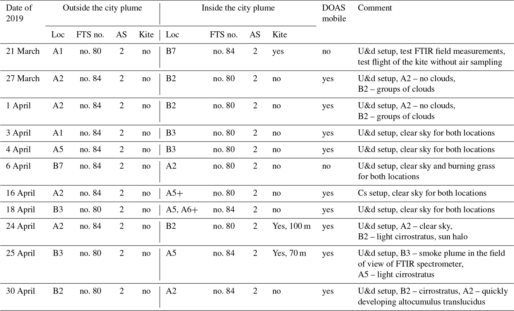
The EMME field campaign in 2019 consisted of 11 d of measurements in March–April. Table A1 (see Appendix A) presents daily information on the location of FTIR spectrometers during the campaign, the FTIR spectrometer identifier, number of bags of air samples, flight of a kite and air sampling altitude. Below, we refer to the two Fourier Transform spectrometers (FTSs) as FTS no. 80 and FTS no. 84. In Table A2 (please see Appendix A) we collect the main characteristics of weather conditions for each measurement day. The satellite images of cloud cover detected by the MODIS satellite instrument in the vicinity of St. Petersburg are presented in Fig. A1 (see Appendix A). They confirm daytime clear-sky conditions for the duration of the campaign, except the day of 30 April, when altocumulus translucidus clouds started to develop.
During EMME-2019 we implemented two types of field experiment setup regarding the position of FTIR spectrometers relative to the dominant air flow (wind) direction:
-
For most of the days of observations (10 of the 11), FTIR spectrometers were installed along the wind direction line – in up- and downwind locations on opposite sides of the city of St. Petersburg (Fig. 1, locations no. 1 and no. 2).
-
For 16 April, the cross-sectional setup was implemented. FTIR spectrometers were located on the line which is nearly perpendicular to the dominant wind direction line (not shown in Fig. 1).
In order to forecast the spatial distribution of urban air pollution on each day of campaign observations, we used the HYSPLIT model. Following our previous experience of simulating the dispersion of urban contamination from St. Petersburg, the NO2 content in the lower troposphere was set as a tracer of the polluted air mass distribution (Ionov and Poberovskii, 2019). This numerical modelling was done by means of the dispersion module within the offline version of HYSPLIT. It allowed the 3-D simulation of the generation and dispersion of the NO2 plume to be performed from a set of given sources of anthropogenic NOx emission. The model was configured in the same way as in our early studies (Ionov and Poberovskii, 2012, 2015, 2017). Similar to the most recent study by Ionov and Poberovskii (2019), the NOx emissions were specified according to the official municipal inventory of emission sources. The HYSPLIT grid domain was set with the centre at 58.20∘ N and 30.75∘ E, the grid spacing (horizontal spatial resolution) of 0.05∘ latitude and longitude and the grid span of 6.8∘ latitude and 14.1∘ longitude. The vertical grid consisted of 10 levels with the tops at 1, 25, 50, 100, 150, 250, 350, 500, 1000 and 1500 m. The forecast meteorology data (vertical distributions of the horizontal and vertical wind components, temperature and pressure, etc.) were taken from the National Centers for Environmental Prediction Global Forecast System (NCEP GFS; ftp://arlftp.arlhq.noaa.gov/forecast, last access: 2 March 2020) on the 1∘ × 1∘ latitude × longitude spatial grid. The maps of the NO2 plume, simulated by the HYSPLIT model for 13:00 LT on each day of campaign observations, are presented in Fig. 3. The colour scale represents the spatial distribution of the NO2 column amount integrated within the boundary layer (∼ 1500 m). An animated version of such a forecast, showing the plume evolution, was generated and shared among the campaign staff ∼ 12 h before each day of planned observations (an example of the animated forecast for 6 April 2019 is available at https://youtu.be/rgtq6JLPhig, last access: 2 March 2020).

Figure 3The HYSPLIT model output for each of the campaign days (10:00 UTC) used as the forecast of the megacity plume while planning the field campaign. The colour bar units for are [0–25] 1015 cm−2. The blue line in the southeast indicates the river Neva.
Based on the plume evolution forecasts, the optimal pair of the FTIR spectrometer locations for the upcoming day of measurements was chosen. This approach to the planning of the city campaign was implemented during 11 d of EMME-2019, and the necessity to change the location of the FTIR spectrometers occurred only once, on 18 April. For this day, the real-time information on the NO2 tropospheric column (TrC) acquired along the ring road by crew no. 3 using mobile DOAS observations showed that the actual location of the most polluted city plume area was different from one which had been predicted by the HYSPLIT simulations. It should be noted that the mobile DOAS observations were organised in such a way that the data on the TrC of NO2 for the location outside the city plume were collected first. There were 2 d of FTIR measurements without mobile DOAS observations due to technical issues. Our experience has shown that the HYSPLIT forecast was precise enough to ensure proper selection of FTIR locations on these days.
4.1 FTIR and DOAS data processing
The dual-channel EM27/SUN spectrometer can measure total column abundances (TCs) of O2, H2O, CO2, CH4 and CO (Gisi et al., 2012; Hase et al., 2016). The processing of the raw FTIR data (generation of spectra from raw interferograms and trace gas retrievals) is performed using the software tools provided by the COCCON (Frey et al., 2019; COCCON, 2019). The required software is open-source and freely available; the development of these tools has been supported by ESA. The interferograms recorded with FTS no. 80 and FTS no. 84 were the main input data. In the first processing step, spectra are generated from the recorded DC-coupled interferograms, including a DC correction (Keppel-Aleks et al., 2007) and quality filtering. In the second processing step, TCs of the target species are derived from the spectra. For the retrievals of the total columns of O2, CO2, CO, H2O and CH4, the spectral regions recommended by Frey et al. (2019) and Hase et al. (2016) were taken. We present these intervals in the respective order: 7765–8005 cm−1 (the main interfering gases are H2O, HF, CO2), 6173–6390 cm−1 (the main interfering gases are H2O, HDO, CH4), 4210–4320 cm−1 (the main interfering gases are H2O, HDO, CH4), 8353–8463 cm−1 and 5897–6145 cm−1 (the main interfering gases are H2O, HDO, CO2). The EM27/SUN spectrometer has a low spectral resolution of 0.5 cm−1. Therefore the TCs are derived from the FTIR spectra through scaling of the a priori profiles of target gases (Frey et al., 2019). The required auxiliary data are the local ground pressure, the temperature profile and the a priori mixing ratio profiles of the gases. For ensuring consistency with the TCCON reference network in this regard, these atmospheric profiles were provided by TCCON. The ratio of the target gas TC to the retrieved O2 TC, which is suggested to be known and constant, gives us the column-averaged dry-air mole fraction (Xgas) of the target gas (Wunch et al., 2011; Frey et al., 2015):
where Xgas is the column-averaged dry-air mole fraction of the target gas (unit: dimensionless quantity), TCgas is the total column of the target gas (unit: ), is the total column of O2 (unit: ) and TCdry air is the dry-air total column (unit: ). Using Xgas helps to reduce the effect of various possible systematic errors (Wunch et al., 2011). To provide the compatibility of EM27/SUN measurements with the WMO scale, and for consistency reasons, the retrieval software used for processing the EM27/SUN spectra also performs post-processing (Frey et al., 2015). Finally, we had both the TCgas and Xgas for each day of measurements at each observational location at our disposal.
For the interpretation of spectral UV–Vis measurements and the derivation of tropospheric NO2 content, the well known DOAS method is used (Platt and Stutz, 2008). Basically, the DOAS algorithm derives the NO2 atmospheric content by fitting a reference NO2 absorption cross-section to the measured zenith scattered radiance. The effective or slant column density (SCD) of NO2 is retrieved in the 425–485 nm fitting window. SCD is converted then to vertical column density (VCD) by means of a so-called air mass factor, AMF (VCD = SCD/AMF), precalculated with a radiative transfer model (RTM). The spatio-temporal variations of stratospheric NO2 are negligible compared to these in a polluted troposphere. Consequently, the variations of NO2 vertical column observed in the data of our mobile DOAS measurements are related to NO2 pollution in the boundary layer (below ∼ 1.5 km). In general, such observations have been proved to be an efficient technique to derive the anthropogenic NOx flux in many studies worldwide (see, for example, Johansson et al., 2008, 2009; Rivera et al., 2009, 2010; Ibrahim et al., 2010; Shaiganfar et al., 2011, 2015, 2017; Wang et al., 2012; Wu et al., 2017).
4.2 Side-by-side calibration of FTIR spectrometers
The target quantity of our observations is the small difference between two large values that are measured by different instruments of the same type. Therefore, a careful cross-calibration of the instruments is of primary importance for the considered experiment. Side-by-side calibrations of FTS no. 80 and FTS no. 84 were carried out on 12 April, 26 April, 15 May and 16 May 2019. The instruments were installed at the observational site of St. Petersburg State University in Peterhof and operated simultaneously for the time period of clear-sky weather, which lasted from half an hour to several hours. The total number of spectra acquired during cross-calibrations was 604. They were collected during about 10 h of simultaneous measurements. The scatter plots showing cross-comparison of the data are given in Fig. 4. For all considered gases (CO2, CH4, CO), the results for column-averaged dry-air mole fractions (Xgas) delivered by the two FTSs are in a very good agreement. The determination coefficients for CO2, CH4 and CO are 0.9999(99), 0.9999(99) and 0.9999(89), respectively. The calibration factors obtained as a result of the side-by-side comparison were used to convert XCO2, XCH4 and XCO measured by spectrometer no. 80 to the scale of spectrometer no. 84. The results of cross-calibration help to avoid an additional source of systematic error in the estimation of area fluxes. The root mean square (rms) differences between time series of simultaneous measurements by FTS no. 80 and FTS no. 84 are equal to 0.10 ppm (0.025 %) for CO2, 0.59 ppb (0.032 %) for CH4 and 0.38 ppb (0.38 %) for CO.
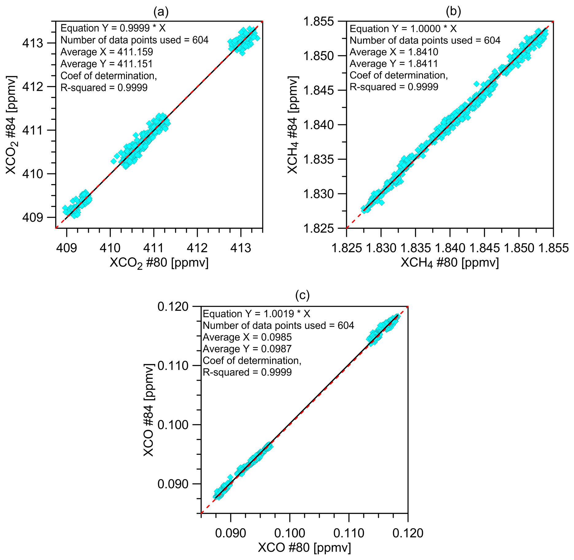
Figure 4The scatter plots of cross-comparison of the average mole fraction data during side-by-side calibrations.
The scaled results of the side-by-side measurements of XCO2, XCH4 and XCO by FTS no. 80 and FTS no. 84 on 12 April 2019 at the St. Petersburg observational site are presented in Fig. 5. The individual results and 15 min running average data are shown. We used the side-by-side measurements for estimating the optimal averaging period for the Xgas data. Averaging is the necessary prerequisite for using these data for the evaluation of emission and for comparison with the results of modelling. It should be emphasised that the data sampling for other input parameters varies considerably. In order that all datasets are consistent, the optimal sampling intervals were determined. For the FTIR measurements, the averaging interval has been selected in such a way that short-term variations of measured quantities can be detected. As an example, we point to three local maxima of XCH4 and XCO during the time period of 13:00–15:00. One can see that these maxima with a half width of about 15–20 min and with amplitudes of ∼ 0.5 ppbv and of 0.1 ppbv for XCH4 and XCO, respectively, are nicely covered as well as the increase of the greenhouse gases around noon, so the chosen value of an averaging interval of 15 min seems reasonable. The chosen averaging interval of 15 min is in good agreement with the estimation of the optimal integration time (10 min) obtained as a result of the Allan analysis implemented by Chen et al. (2016). Chen et al. (2016) applied this approach for the differential measurements of XCO2 and XCH4 performed by three EM27/SUN spectrometers within urban areas.

Figure 5The scaled results of the side-by-side measurements of XCO2, XCH4 and XCO by FTS no. 80 and FTS no. 84 on 12 April 2019.
4.3 Mass balance approach for area flux estimation
The estimation of the area fluxes F was obtained on the basis of a mass balance approach implemented in the form of a one-box model. Box models are a widely used technique for the evaluation of urban and other emission fluxes (Hanna et al., 1982; Reid and Steyn, 1997; Arya, 1999; Zinchenko et al., 2002; Zimnoch et al., 2010; Strong et al., 2011; Hiller et al., 2014a; Chen et al., 2016; Makarova et al., 2018). In our case the following equation for the calculation of area flux was used:
where F (unit: ) is the area flux, and ti denotes the day of a single field experiment in the frame of the observational campaign. It should be emphasised that we used the steady-state approximation for all processes involved within the duration of a single field experiment, so ΔTC (unit: ) is the mean TC difference between downwind (TCd) and upwind (TCu) observations ΔTC = TCd − TCu, V (unit: m s−1) is the mean wind speed and L (unit: m) is the mean length of a path of an air parcel which goes through the urban territory of St. Petersburg agglomeration. The k coefficient converts the value of area flux from units of to units of :
where mgas is the molecular mass of the target gas (unit: kg mol−1), NA is the Avogadro constant (unit: mol−1) and 31536 × 106 is the coefficient that converts the value of area flux from units of to units of . The data for the wind speed and the wind direction were taken from different sources of meteorological information (see Sect. 4.3), and these sources are identified as j in Eq. (2). So, as a result, we obtained the set of values of F(t) for each of the meteorological data sources and for each day of field measurements. We note that below we will use the units for the values of F(t).
4.4 Wind field data
Obviously, reliable wind field information is an important prerequisite to get an accurate estimate of the target emissions from the data of remote spectroscopic measurements. For instance, it has been noted by Ionov and Poberovskii (2015) that the uncertainty of the surface wind direction is the main contributor to the total error of NOx emission by the megacity of St. Petersburg, estimated from circular DOAS measurements. It was also found that the direction of the surface wind acquired by ground-based meteorological observations often does not match the results of modelling of the pollution plume and the results of the NO2 mobile measurements (Ionov and Poberovskii, 2017). Apparently, the routine wind observations in the city are subject to significant local perturbations due to unavoidable interactions of the wind flow and the adjacent city buildings. It should be emphasised that the HYSPLIT simulations of the fields of tropospheric NO2 demonstrate reasonable agreement with the plume dispersion observed by the circular mobile observations (Ionov and Poberovskii, 2017, 2019). The latter is also true for plume simulations, presented in the current study in Fig. 3. However, one can easily notice inconsistencies between the dominant directions of plume movement and the surface winds as specified in Table A2 (see Appendix A): e.g. on 21 and 27 March and 1 and 24 April, when the city plume was moving towards southeast but the surface wind was west-southwest (see Fig. 3). In order to get more accurate wind information, we have considered additional sources of wind data:
-
in situ measurements of a Vaisala WXT520 weather transmitter with an ultrasonic wind sensor, installed locally on the roof of the building of the Institute of Physics of SPbU (∼ 60 ; 59.88∘ N, 29.83∘ E; point A1 in Fig. 2), hereafter referred to as “LOCAL”;
-
the data of Global Data Assimilation System (GDAS) from the NCEP GFS model, which is similar to the one used to initialise the HYSPLIT dispersion calculations as specified in Sect. 3, hereafter referred to as “GDAS”;
-
the wind speed and direction data retrieved from the backward trajectory calculations of HYSPLIT at the location of downwind FTIR observation, hereafter referred to as “HYSPLIT”.
We selected HYSPLIT as one of the sources of the wind data since HYSPLIT is a widely used modelling system for the simulation of air parcel trajectories and the dispersion processes in the atmosphere which was tested in a lot of studies (HYSPLIT publications can be found using the following links: https://www.arl.noaa.gov/hysplit/hysplit-publications-meteorological-data-information/, last access: 2 March 2020). Stein et al. (2007) noted the following:
Grid models are the best-suited tools to handle the regional features of these chemicals. However, these models are not designed to resolve pollutant concentrations on local scales. Moreover, for many species of interest, having reaction timescales that are longer than the travel time across an urban area, chemical reactions can be ignored in describing local dispersion from strong individual sources making Lagrangian and plume-dispersion models practical.
Stein et al. (2007) classify HYSPLIT as a local model which provides “the more spatially resolved concentrations due to local emission sources”. Therefore, for modelling of the evolution of the St. Petersburg plume we used the HYSPLIT model as a tool which perfectly fits the scale of considered atmospheric processes. This was also the reason for using HYSPLIT as the source of the wind data.
Both GDAS and HYSPLIT wind data are taken at the altitude level that approximately corresponds to the middle of the daytime boundary layer height. An average wind is calculated for the time period of FTIR observations. Resulting wind speeds and directions from the three different data sources are given in Table A3 (see Appendix A). As expected, wind speeds at elevated altitude levels from GDAS and HYSPLIT are much higher than the surface wind speeds (see Appendix A, Table A2). On some days, e.g. 6 and 18 April, in situ wind directions (LOCAL) differ considerably from GDAS and HYSPLIT, although the latter two are consistent with each other. Note that compared to surface, the elevated wind directions better reproduce the city plume movement – e.g. northwest winds and west-northwest winds on 21 and 27 March and 1 April (see Fig. 3) instead of west-southwest winds at the surface (see Appendix A, Table A2).
4.5 Air parcel path length
The determination of the air parcel path length L (Eq. 2) is a sophisticated task due to the fact that the application of a box model suggests that the pollutants are well mixed in the entire air box volume, but this is not true, especially for megacities with a complex structure of urban terrain and distribution of emission sources. Thus, different approaches have been tested to calculate L:
-
A simplified box model setup with a constant path length was employed for each day of field observations. The box is designed to represent the major part of the high-density residential and industrial area of the St. Petersburg agglomeration, so that the respective L value is derived from the value of that area. Since the locations of our field observations are mostly placed on the outer side of the ring road, this road was set to be a boundary for the target emission area. Accordingly, given that the land area inside the ring is equal to 706 km2, we get an estimate of ≈ 27 km. Hereafter the results of data interpretation by means of this approach are indicated by “Lconst”.
-
The variable effective path is calculated using the actual wind direction and the land use pattern on the route of the linear air trajectory. Only those sections of path are being taken into account that cross the area of supposed anthropogenic emission. The input wind directions are those mentioned in Table A3 (see Appendix A), and the resulting path length calculations hereafter are indicated as “LLOCAL “, “LGDAS” and “LHYSPLIT”. The use of the effective path in Eq. (2) takes into account the inhomogeneity of the anthropogenic emissions in the megacity to some extent.
For the purpose of effective paths calculation, a special gridded model of land use coverage has been constructed on the basis of the visual classification of a publicly available map (https://yandex.ru/maps/2/saint-petersburg/?ll=30.163886%2C59.911377&z=11, last access: 28 January 2020) that covers the St. Petersburg agglomeration with its surroundings (see Fig. 6). The spatial domain of the model covers 76 km in a south–north direction and 128 km in an east–west direction (59.60–60.29∘ N, 29.05–31.33∘ E). It has been assumed that there are no significant emission sources outside this domain. The model resolution (grid size) is 25 m × 25 m. The following major land use classes are considered: residential buildings/industrial areas, roads/highways, water bodies, parks/forests/fields and swamps/wetlands. In Fig. 6 these land use classes are shown in different colours: blue for the water bodies, grey for the residential buildings/industrial areas and green for the parks and forests. Effective path length is calculated as the sum of elementary paths through the urbanised grid pixels which contain residential buildings, industrial areas and roads/highways. Pixels containing water bodies, swamps and parks are excluded from the variable path calculations. A similar approach was implemented by Hase et al. (2015). The total urbanised area of the St. Petersburg agglomeration according to the developed land use classification occupies the area of 984 km2, while the entire area of St. Petersburg is officially reported to be 1439 km2. The target gases can originate from different emission source categories; i.e. CH4 could partly come from the waterways (sewers and water canals), wetlands and pipelines rather than mobile and point combustion sources which are relevant for CO, CO2 and NO2. The EMME-2019 was carried out during March–April when the water bodies and earth surface were fully or partly covered by ice and snow (see Appendix A, Fig. A1), and soils were still frozen. Therefore we suggest that CH4 emission from the excluded pixels (water bodies, swamps, parks, and forests) was negligible in comparison to other anthropogenic sources (landfills, pipelines and sewage treatment plants, etc.) which are distributed over the urbanised pixels.
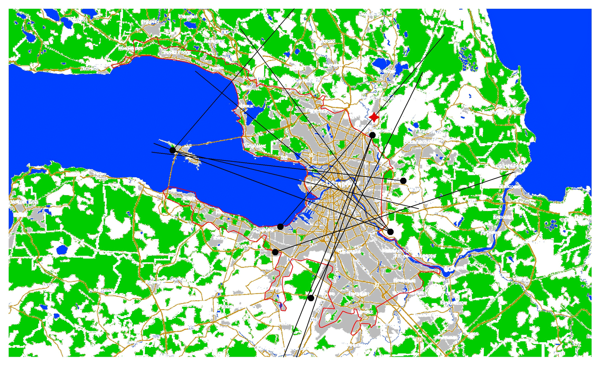
Figure 6An example of linear backward paths (black straight lines; black dots show the downwind FTS locations) for the days of FTIR observations. The major land use classes are shown by different colours (blue for the water bodies, grey for the residential buildings/industrial areas and green for the parks and forests). The path lengths on the map are plotted as equal only for illustrative purposes. In fact they are all different since the FTIR observation locations and the wind field change from day to day. The red line designates the official administrative boundary of the St. Petersburg agglomeration. The red star indicates the location of a the major thermal power station (TPS) located to the north of St. Petersburg. Map data © 2019 Yandex.
To minimise errors that may occur due to the land use misclassification, and to take into account the airflow spatial extension, the 10 km wide band of 11 equidistant and parallel paths is analysed, and an average path length is calculated. Finally, the difference between the “polluted” path (backward from the downwind location) and “clean” path (backward from the upwind location) provides an estimate of the effective path L. Figure 6 presents an example of linear backward paths for the days of FTIR observations with the major land use classes shown by different colours.
4.6 Case study: two examples
In order to illustrate the interpretation of experimental data and describe the main error sources of final results, we consider 2 d of field measurements. The first one, 4 April, seems to be the most successful in terms of observational conditions, functioning of the equipment, data quality and clarity of the interpretation. It is characterised by stable weather conditions with a moderate south-southwest wind, similarly identified by different wind data sources – from the surface (see Appendix A, Table A2) to higher altitude levels (see Appendix A, Table A3). The simulated city plume picture demonstrates a jet-like flow of air mass on that day, with an almost perfect location of both FTSs, upwind and downwind almost on one line (see Fig. 3). In addition, according to the model simulation for 4 April, the upwind FTS was located in the clean area, while the downwind one was installed very close to the plume jet. Another example is 25 April, when both FTS locations appeared to be inside the polluted area. This happened due to the specific weather conditions that contribute to the accumulation of air pollutants in the boundary layer: a calm night before and light winds of 1 m s−1 in the daytime (see Appendix A, Tables A2 and A3). Moreover, the wind direction on 25 April at the surface (south-southwest, Table A2) is very different from that in the middle of the boundary layer (east and east-northeast; Table A3).
According to the analysis of the air samples collected in air bags, the surface air on 25 April was extremely polluted. The downwind NO2 concentration was found to be 138 µg m−3, while it was varying within the range of 12–74 µg m−3 during the other days of field observations. Another indication of heavy anthropogenic pollution comes from the data of our mobile DOAS measurements: the maximum of NO2 TrC recorded along the circular route was 92 × 1015 on 25 April, while it was in the range of 15–58 × 1015 on the other days of field observations. According to the data of municipal air quality monitoring, the daily average concentration of the particulate matter (PM10) was very high and exceeded 60 µg m−3 (http://www.infoeco.ru/, last access: 4 March 2020). A high-pollution event was also recorded by the CIMEL sun photometer installed at St. Petersburg State University (point A1, Fig. 2) within the AERONET international programme (Volkova et al., 2018): the daily averaged value of aerosol optical thickness (AOT) at 500 nm was found to be 0.40 on 25 April, which is considerably higher than its long-term average value (0.12 for the period of 2013–2019); a similar increase of AOT was recorded by the satellite measurements of the MODIS satellite instrument over St. Petersburg on that day.
The TC data of CO2 measurements on 4 and 25 April, with 15 min running averages, are presented in Fig. 7. Compared to 4 April, the TC of CO2 on 25 April demonstrates higher levels and variation, both at upwind and downwind locations. Although the upwind TC is generally below the downwind level, as expected, the upwind TC starts to exceed the downwind level at the end of FTS observations on 25 April. Accordingly, while the “downwind–upwind” difference is relatively stable within the range of 2–4 × 10¹⁹ on 4 April, it reaches 10 × 1019 at 12:00 on 25 April but becomes zero and then negative (up to −1 × 10¹⁹ ) after 14:30. In order to explain this behaviour, a special run of the HYSPLIT dispersion model was performed, with an output of CO2 TC within a boundary layer every 15 min, at both FTS locations, upwind and downwind (see Fig. 7). As the first approximation, the CO2 emission sources were assumed to be located similarly to the NOx emission sources but scaled to match the level of our FTS measurements. These calculations qualitatively reproduce the time series of the CO2 measurements and the different character of the results of field experiments on 4 and 25 April. Moreover, we can suggest that the origin of high CO2 TC values observed at the upwind FTS location on 25 April was the thermal power station located about 5 km towards north from the upwind point (see Fig. 6). When the emission by the thermal power station is turned off in the HYSPLIT calculation, the CO2 TC drops down to the level of upwind FTS measurements on 4 April (see Fig. 7b, dashed blue line).
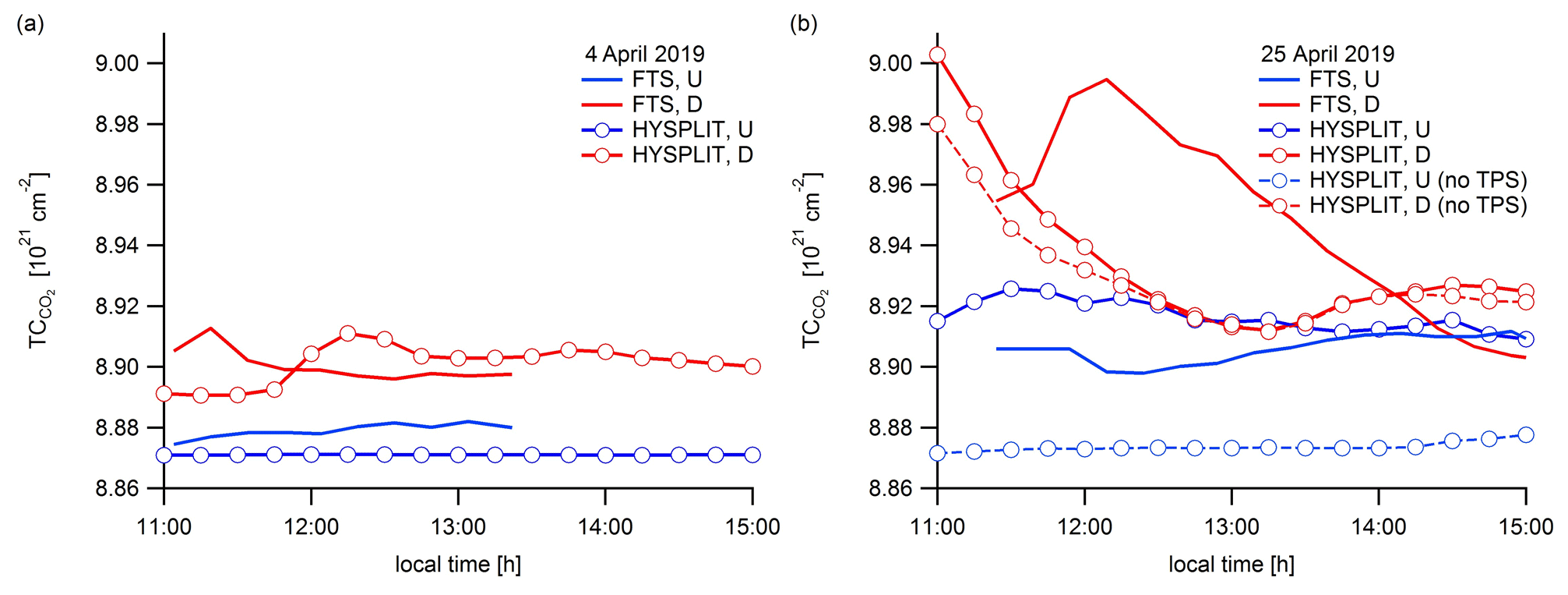
Figure 7Time series of the CO2 TC measurements by mobile FTSs at upwind (U, blue) and downwind (D, red) locations on 2 d, (a) 4 and (b) 25 April 2019. The measurements are compared with the results of the HYSPLIT simulations at both locations, upwind and downwind. For the day of 25 April, a special HYSPLIT scenario is added for comparison: the emission of the major thermal power station (TPS) of St. Petersburg nearby the upwind FTS location is turned off (“no TPS”; see Fig. 8 and the text for details).
The time series of Xgas for CO2, CO and CH4 obtained from the data of FTS measurements on 4 and 25 April are shown in Fig. 8. Since the Xgas variability at clean location (upwind) is usually much smaller as compared to a polluted location, it is possible to use time extrapolation of measured data for the periods with data gaps. Figure 9 demonstrates the difference between TC for each of three gases measured by upwind and downwind FTS on 4 and 25 April; the extrapolated data are specially marked. Figure 9 also shows the wind speed and wind direction for the time period of FTS observations by the LOCAL weather station (see Sect. 4.3).

Figure 8Time series of Xgas for 4 April (a) and 25 April (b) at the clean location of FTSs (blue dots) and at the polluted location of FTSs (red dots). Solid lines of corresponding colours denote the 15 min running average.
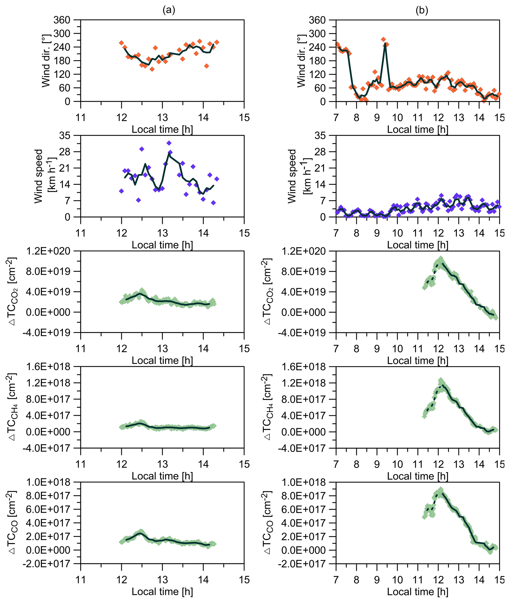
Figure 9The difference between the TC values at the polluted and clean locations of FTSs on 4 April (a) and 25 April (b). The wind speed and direction are also shown. Solid lines denote the 15 min running average. Dashed lines denote the time interval when extrapolated input data from the clean location were used (see text).
5.1 Overview of obtained results
The campaign consisted of 11 d of field measurements. On 30 April clouds (altocumulus translucidus) started to develop quickly during the field experiment (see Appendix A, Table A1 and Fig. A1). On 18 April the upwind FTS location was close to the thermal power station. Owing to the prevailing north-northeast wind (see Appendix A, Table A3), the upwind FTS location appeared to be polluted on 18 April (see Fig. 3). Consequently, 18 and 30 April were excluded from final analysis, and the evaluation of the target fluxes (F) of the investigated gases was limited to the remaining 9 d of campaign. For these 9 d the cross-correlations (Pearson's correlation coefficient r) between ΔTC values obtained for the pairs and were calculated: = (0.88 ± 0.02) and = (0.82 ± 0.03). The high correlation is the evidence of the fact that the measurements in most cases were conducted inside the plume coming from a regional/mesoscale, relatively compact powerful source of emission. We can attribute this source to the centre of St. Petersburg.
To further consolidate our flux estimates, some additional restrictions were imposed on the experimental data, which resulted in keeping only 4 d out of 9: 21 and 27 March and 3 and 4 April. The first requirement was the wind field stability. The analysis of the wind field stability during each day was carried out using the GDAS and HYSPLIT meteorological data, as well as local meteorological observations. The second criterion was the homogeneity of the megacity pollution plume. It was estimated on the basis of the analysis of the daily variability of enhancement ratios . The EnhR values for the following pairs were considered: and . For selected days, the upper limit of the daily relative variability of EnhR was set to 30 %.
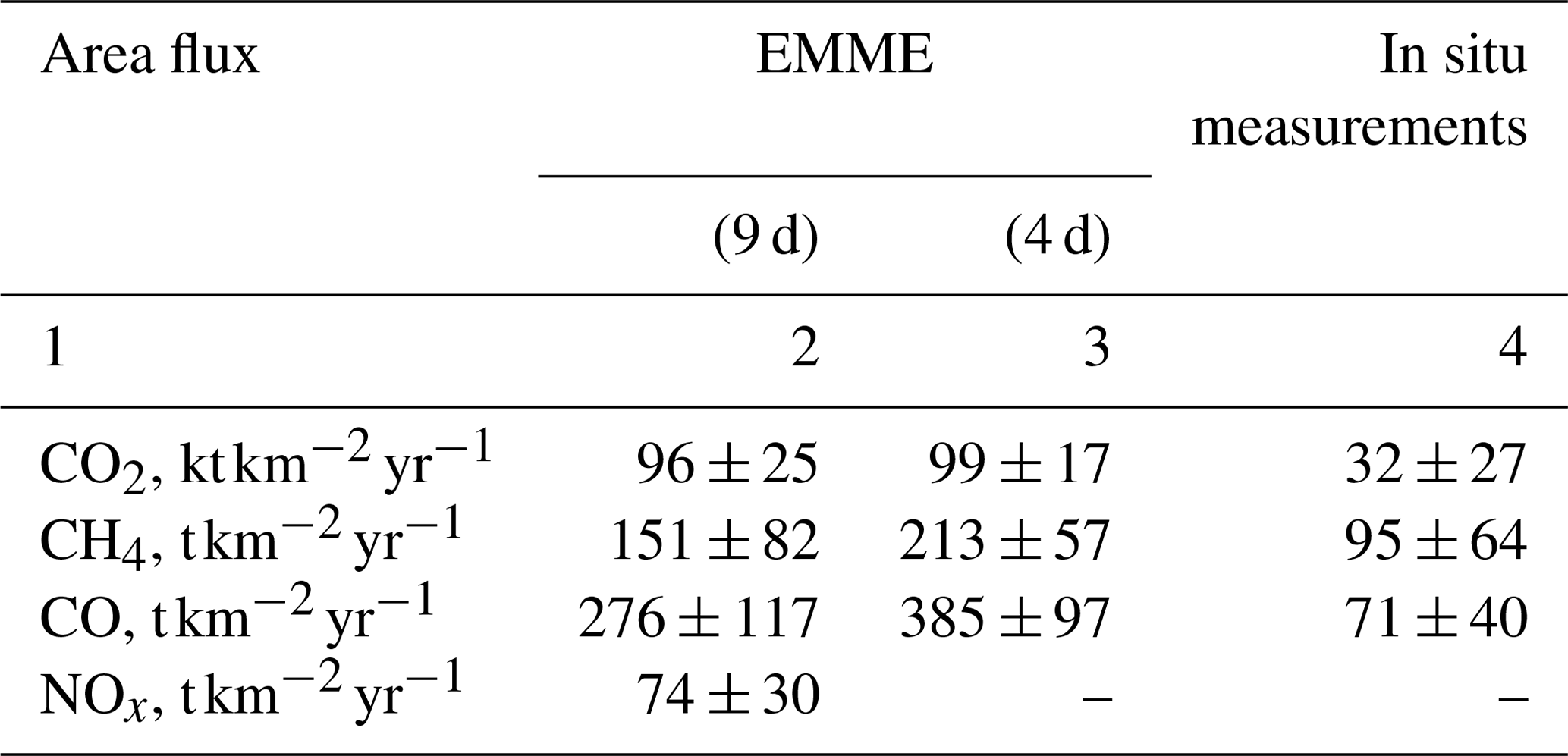
As has been described above, there were several different scenarios of the F calculations in which different sources of meteorological information (LOCAL, GDAS and HYSPLIT) and different methods of the air parcel path calculations were used. The comparison of the obtained results has shown that the minimum variability of F is observed when the HYSPLIT meteorological data are combined with the variable effective path L (see Sect. 4.5). When selecting the results for final analysis, we suggest that the application of the criterion of minimal variability is a good choice because in this case the corresponding estimates of area flux are more reliable. This statement can be confirmed in particular by comparison of the CO2 fluxes obtained for the 9 and 4 d sets (Table 1, columns 2 and 3). For the 4 d set, the variability is considerably lower (12 vs. 28 ), and we should reiterate that these 4 d were the days with the most favourable observational conditions during the observational campaign. So, we do not present the results of all scenarios and show in Table 1 (columns 2 and 3) the values obtained for the combination of HYSPLIT meteorological data with the variable effective path. As supplementary information, in Appendix B we provide Table B1, which contains the values of area fluxes for CO2, CH4, CO and NOx obtained using the constant path length approach.
If we compare the flux values obtained for the 4 and 9 d sets, we see that the fluxes for CO2 are the same, but the fluxes for CH4 and CO are different (Table 1, columns 2 and 3). The fluxes estimated for the selected 4 d appeared to be 1.3 times higher than corresponding values obtained for all 9 d of field observations. The uncertainty of the obtained flux values for the 4 d subset decreased for CO2 and CH4. We stress that during these selected 4 d not only did the specific meteorological conditions correspond in the best way to the assumptions of the box model, but also the locations of the observational points were nearly perfect.
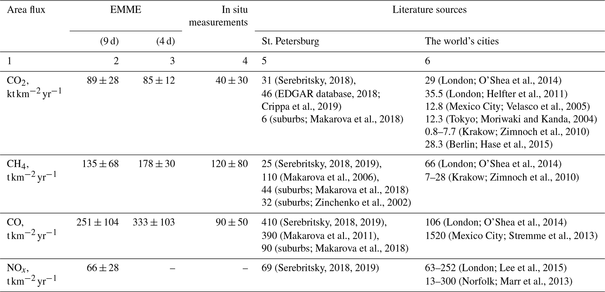
Table 1Area fluxes for CO2 (), CH4 (), CO () and NOx () obtained during EMME-2019 and the flux estimates for St. Petersburg based on in situ measurements. The values previously reported in literature are also presented.
The summary of the EMME-2019 results and the comparison with the flux estimates for St. Petersburg based on in situ measurements, as well as independent literature data, are presented in Table 1 for CO2, CH4, CO and NOx (the latter were derived from mobile DOAS measurements of tropospheric NO2 in the vicinity of upwind and downwind FTIR observations). Prior to analysis of the results, a short overview of the error and uncertainty analysis should be presented. The random uncertainty of mean F values of CO2, CH4, CO and NOx indicated in Table 1 was calculated as the standard deviation (SD) of daily means of area fluxes. This uncertainty includes two components. The first component is the natural flux variability, and the second component comprises the random measurement errors and the errors introduced by approximations and simplifications of the model approach which was used. It should be specially emphasised that these two components cannot be identified separately. Therefore, below we will use the terms “variability” or “uncertainty”, keeping in mind that these terms denote natural variations, measurement errors and model errors together. The relative random uncertainty of F for a single day of measurements (daily uncertainty) can be estimated using the following expression:
where δVis the relative variation of the wind speed over a day estimated using HYSPLIT meteorological data, δL is the relative uncertainty of the air parcel path length and δΔTC is the relative daily variation of ΔTC. The δF values calculated in this way can be considered as an upper limit of the F uncertainty. The average values of δL, δV and δΔTC estimated for 9(4) d of the city campaign are as follows: δL = 23(24) %, δV = 23(13) %, ΔTC(CO2) = 33(28) %, ΔTC(CH4) = 50(22) % and ΔTC(CO) = 42(28) %. Finally, the average values of the relative daily uncertainty of area fluxes are equal to = 79(65) %, = 96(59) % and δFCO = 88(65) %. As an example, daily mean values of the CO2 area flux obtained during the city campaign are presented in Fig. 10, where the error bars are the random uncertainties of F values derived from corresponding relative mean uncertainties for 9(4) d sets.
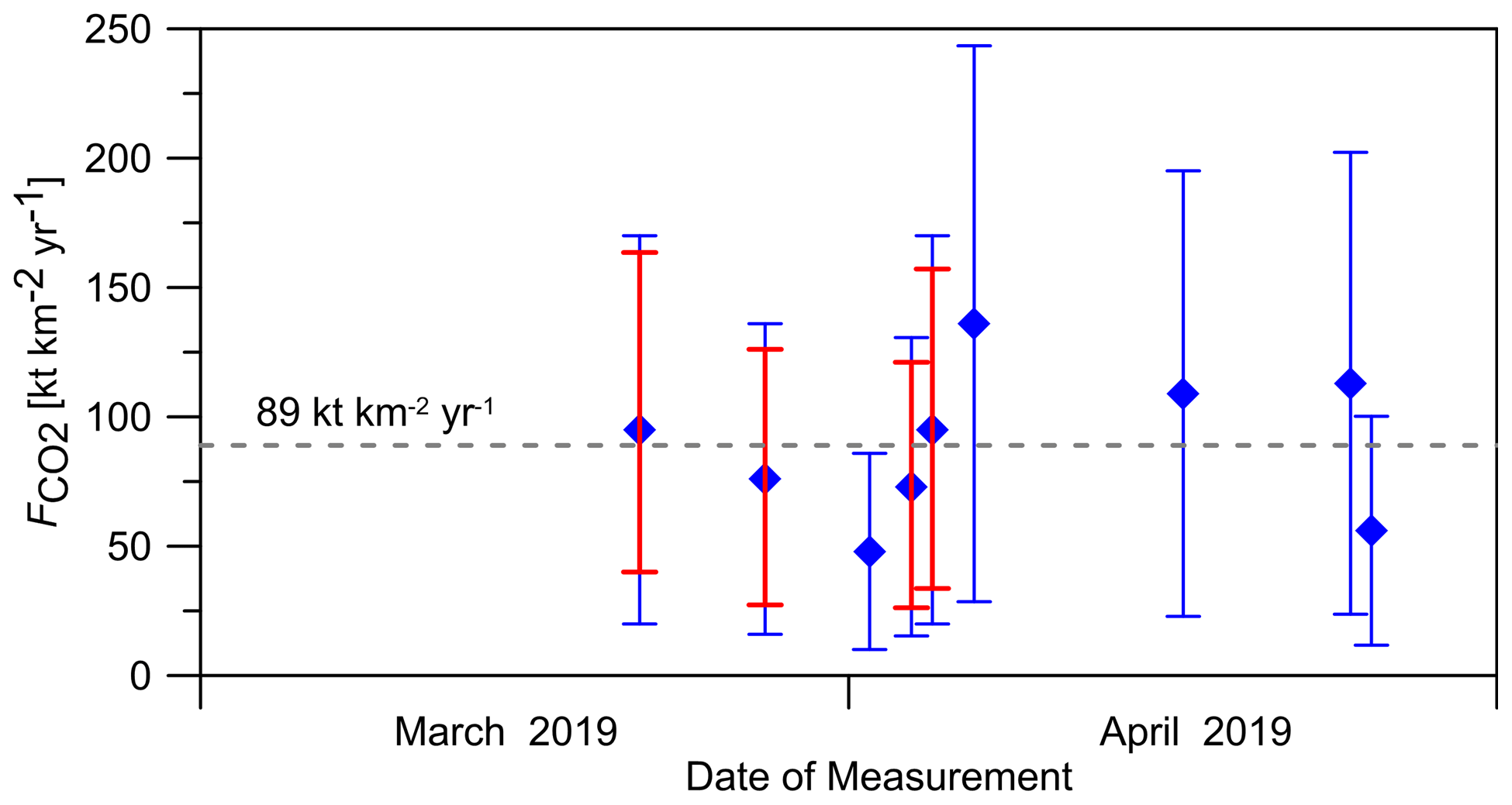
Figure 10Daily mean values of the CO2 area flux F obtained during the city campaign. Error bars show the uncertainties of F values estimated for the 9 and 4 d datasets (blue and red, respectively).
To evaluate the systematic error of the area flux (δFsys) we should first estimate the systematic errors, δLsys, δVsys and δΔTCsys, of corresponding parameters, L, V and ΔTC, in Eq. (2). In contrast to δLsys and δVsys, the contribution of systematic component of δΔTCsys into δFsys is negligible. This is due to the high accuracy of the COCCON observations of gas columns which are calibrated against the WMO scale. In Eq. (2) we use an assumption that an air parcel moves along a straight line, but obviously this is not true. For the whole ensemble of HYSPLIT trajectories simulated for all days of the city campaign, we calculated the maximum relative difference between the true lengths of HYSPLIT trajectories and our straight line approximations of L. This value is equal to ∼ 4 %, which is considered to be an estimation of the relative systematic error δLsys. According to the information on wind speed (see Appendix A, Table A3) observed during the field campaign, the mean relative difference between HYSPLIT and GDAS data on wind speed is of 14 ± 22 %. Hence, the estimation of the systematic error of area flux δFsys due to the systematic errors of all parameters in Eq. (2) gives the value 18 %.
5.2 Estimation of the CH4 emissions by means of in situ measurements of its mixing ratio
The fourth column of Table 1 contains the estimations of F for the territory of St. Petersburg, which were made on the basis of the joint analysis of the CH4 local concentrations monitored in the ambient air during March–April 2013 and April 2019 at the SPbU atmospheric monitoring station (point A1) (Makarova et al., 2018) and Voeikovo station (59.95∘ N, 30.70∘ E; 72 ) of the Voeikov Main Geophysical Observatory (MGO) (Zinchenko, 2002). The CH4 measurements are carried out by MGO in accordance with WMO recommendations for GAW stations (WMO, 2009, 2014). The high quality of the data obtained by MGO is confirmed by the results of WMO/IAEA Round Robin Comparison Experiment 2014/15 (https://www.esrl.noaa.gov/gmd/ccgg/wmorr/wmorr_results.php, last access: 3 March, 2020). The data of Voeikovo station together with 17 other European stations were used to estimate European methane emissions in the framework of the InGOS project (Bergamaschi et.al., 2018). The measurements of these stations have been rigorously quality-controlled (Lopez et al., 2015; Schmidt et al., 2014). The Voeikovo measurements are calibrated against the NOAA-2004 standard scale (which is equivalent to the World Meteorological Organization Global Atmosphere Watch WMO-CH4-X2004 CH4 mole fraction scale) (Dlugokencky et al., 2005). The comparability of the SPbU and Voeikovo station data was ensured by calibrating the SPbU equipment against the working standard prepared by MGO.
Table 2Emission ratios (ER), obtained during EMME-2019 and the ER estimates for St. Petersburg based on in situ measurements. The values previously reported in literature are also presented. In columns 2, 3 and 4, the values of the correlation coefficient (r) for corresponding datasets are given in parentheses.
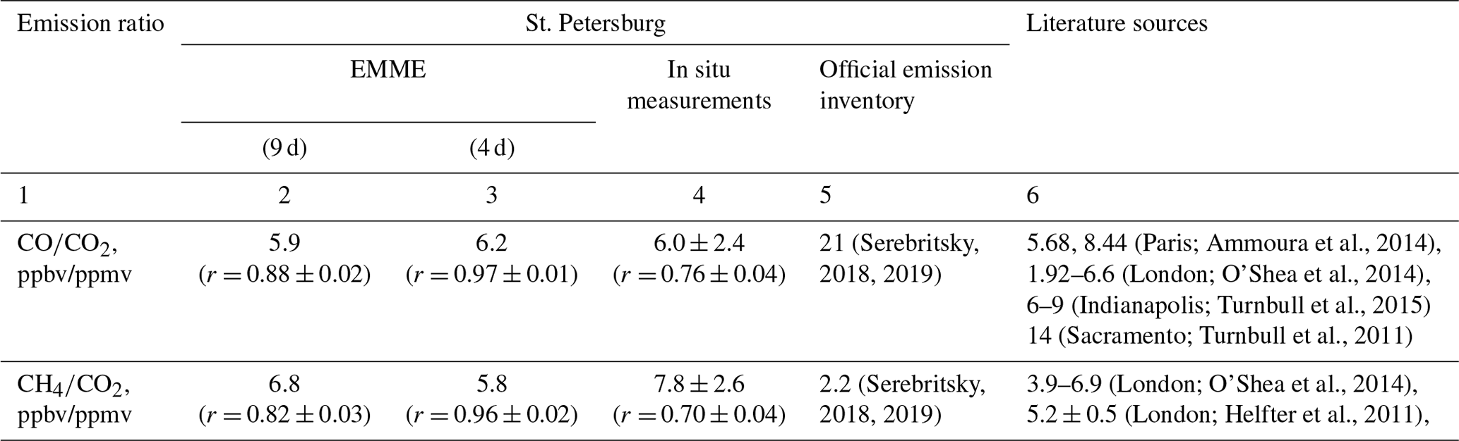
Table 3Comparison of the gas concentrations in air samples collected at the surface and elevated levels on 24 April 2019 and 25 April 2019 at the locations of FTS measurements inside the city plume.
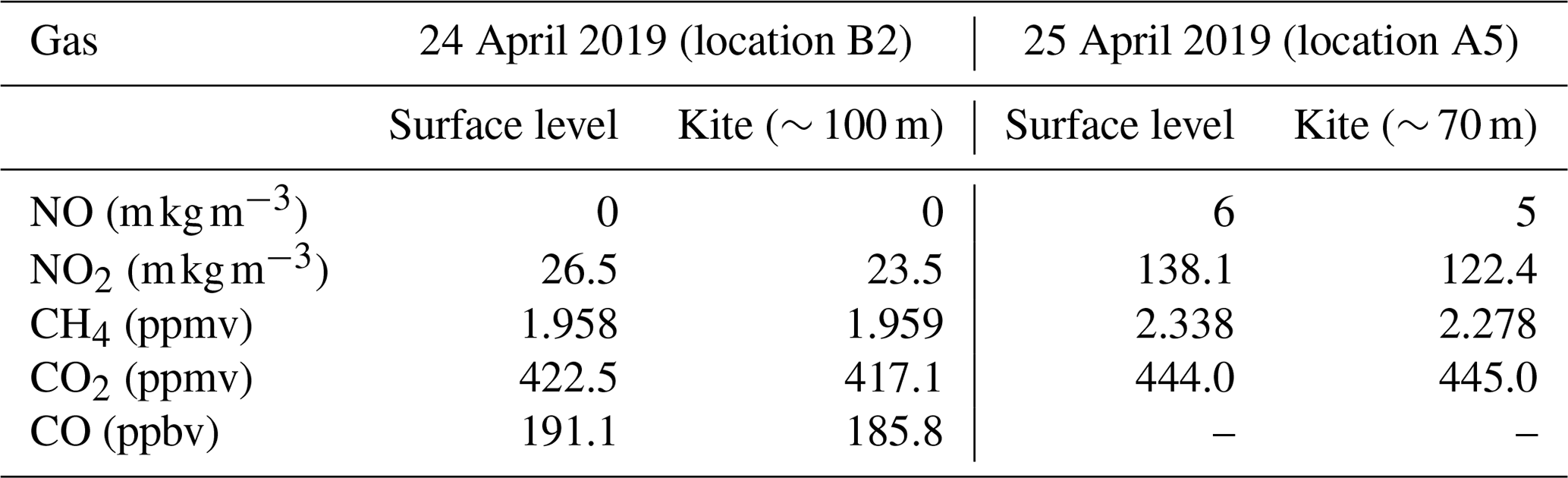
Determination of the CH4 fluxes is possible due to the beneficial location of the observational stations of SPbU and MGO – on the western and eastern sides of the megacity. For the wind directions of 75–85 and 255–265∘, the air mass on the way from one station to another passes through the centre of St. Petersburg. It should be emphasised that only the time periods with the wind speed of at least 2.5 m s−1 were considered. Using the difference in the CH4 concentrations obtained at the monitoring stations, it is possible to estimate the CH4 flux for the central part of the St. Petersburg agglomeration on the basis of a simple box model similar to that used in the present work. It was assumed that all contaminations emitted by St. Petersburg into the atmosphere stay within the boundary layer. The calculation of the variable effective path L between these two monitoring stations gives (21 ± 7) km. The HYSPLIT backward trajectory outputs were used as a source of meteorological data (wind field, boundary layer height data). Finally, the F values for CO2 and CO were estimated using the obtained average CH4 flux (120 ± 80 ) and average EnhR values derived from the in situ measurements of the CO2, CH4 and CO concentrations at SPbU atmospheric monitoring station (point A1) in 2013–2019 (Table 2, the third column). The flux values for CO2 and CO evaluated in this way are 2–3 times lower than the corresponding results of EMME-2019. First, we should emphasise that in situ measurements are more sensitive to very local effects and therefore less representative when compared to column observations. And second, this difference can be partially explained by the presence in the territory of St. Petersburg of a significant number of elevated stationary sources of CO2 and CO – industrial and power/heat plant chimneys (chimneys of the power plant stations can have a height of ∼ 200 m), which emit products of combustion and oxidation of various types of fossil fuels. The effect of elevated sources on gas concentrations measured at the surface layer is often minimal, but this impact can be considerable for total/tropospheric columns and can be detected using remote sensing techniques such as those used during the Berlin campaign (Hase, et al., 2015) and EMME-2019. We present more discussion on this topic in Appendix C. In order to detect the presence of the elevated sources, the air sampling using kite launches was performed during EMME-2019. The air sampling using the kite launching technique was possible only twice when suitable wind speed conditions occurred and there was enough free space for launching. The results of comparison of the gas concentrations in air samples collected at the surface and elevated levels on 24 and 25 April 2019 at the locations of FTS measurements inside the city plume are presented in Table 3. In most cases the concentrations of considered gases at the elevated level are lower when compared to the surface level. There were only two cases with the concentration enhancement in the air samples collected by the kite: for CH4 on 24 April and for CO2 on 25 April; however these enhancements were negligibly small (1 ppbv for CH4 and 1 ppmv for CO2). So, one can come to the conclusion that these two kite launches revealed no elevated pollution plumes.
5.3 Comparison with inventories
Official reports on the environmental conditions of St. Petersburg (Serebritsky, 2018, 2019) contain information on the annual emissions of CO2, CH4, CO and NOx for the entire territory of the metropolis. For comparison with our flux estimates, these total rates were divided by the urbanised area of St. Petersburg (984 km2; see Sect. 4.5). The best agreement of the results of the EMME-2019 campaign with the official emission inventory was obtained for NOx and CO. For NOx, the results of the field campaign and the official emission inventory demonstrated close values: 66 and 69 . The average CO flux for the territory of St. Petersburg, according to official data, is 410 , which is higher in comparison with the values obtained in the current work (251–333 ). At the same time, significant differences in the F estimates for CH4 and CO2 were obtained: the official data are by 5–7 and 3 times lower than the corresponding values obtained during field observations in March–April 2019. Hiller et al. (2014a) showed that the application of the boundary layer budget approach in the form of a box model could give the CH4 area fluxes about 1.5–2 times higher in comparison with corresponding values estimated using the eddy covariance technique and 2.5–6 times higher than F derived from the emission inventory data.
The results of independent studies of anthropogenic emissions reported in the scientific literature show that the estimates of the CO2, CH4, CO and NOx fluxes can vary in a very wide range depending on season, meteorological situation, location of observation points, measurement technique and approach used for estimation of emission (Vaughan et al., 2016; Hiller et al., 2014a; and also see the references indicated in Table 1). The CO2 flux for the St. Petersburg agglomeration obtained in this paper is approximately 3 times higher than for London and Berlin and ∼ 7 times higher than for Tokyo and Mexico City (see Table 1). We would like to note that when comparing the results of different observational campaigns, one should pay attention to the seasonal features of emissions. For example, the Berlin campaign took place in early summer when space heating was off. The EMME-2019 campaign in St. Petersburg was carried out in March–April. The space heating in St. Petersburg is mainly organised in a system of district heating, which is running in the winter mode during this period. The district heating in St. Petersburg is usually turned off at the beginning of May. For CH4, the emission intensity is about 2–3 times higher than the results for London. The CO fluxes for megacities, according to published data, can demonstrate a wide range of values, for example, varying from 106 (London) to 1520 (Mexico City). This range covers our estimates for St. Petersburg: ∼ 251–333 .
One of the most important characteristics of the air pollution source is the emission ratio ERgas1/gas2:
where Fgas is the gas flux, Mgas is the molecular weight of gas. For gases, such as CO2, CH4 and CO, whose lifetime in the troposphere is significantly longer than the duration of field measurements (several hours), the following equality is valid: ER=EnhR. The ER values obtained from the results of the EMME-2019 campaign and in situ measurements at the SPbU atmospheric monitoring station (point A1) in 2013–2019, as well as ER calculated for the official emission inventory and the ER taken from literature, are presented in Table 2. The emission ratios for St. Petersburg obtained as a result of the EMME-2019 campaign and of the in situ monitoring of CH4 at the observational stations located near St. Petersburg have similar values, which are in good agreement with the information on ER for the world's largest cities reported in literature. For the official emission inventory, the ER values for and correspond to the upper and lower limits of the given literature data, respectively. Thus, the relative contributions of CO2, CH4 and CO to the total emissions of the St. Petersburg agglomeration are very similar to the corresponding values for the world's megacities.
5.4 Identification of problems
When studying the application of the remote sensing instruments to the problem of the air pollution meteorology, Beran and Hall (1974) noted the following:
Every urban region is a unique entity and the correct location and sensor distribution for one city may be totally unacceptable for another. Certain features are, however, common to all and can be used to generate a hypothetical city.
Such a hypothetical city usually contains industrial region and line sources of emission in the form of highways. Beran and Hall (1974) also made the following important remark:
Terrain features are another important influence on urban meteorology, many times controlling the local flow which advects or concentrates effluent in a given region. For example, a river valley is a natural place for cold air drainage, while a coastline produces local land and sea breeze circulation, alternately cleansing a region and concentrating pollution at the sea breeze front.
All these mentioned terrain features are present in the territory of the St. Petersburg agglomeration. St. Petersburg is located at the estuary of the Neva River, which flows to the Gulf of Finland. The territory of St. Petersburg occupies northern, eastern and southern coastlines of the Gulf of Finland (Fig. 2). About 40 km to the northeast of the centre of St. Petersburg, the southern coastline of the Ladoga Lake is located. The Ladoga Lake is the largest lake in Europe. All these facts define the weather and climate in St. Petersburg. The complex terrain of the St. Petersburg agglomeration requires special attention due to its influence on the air pollution meteorology.
The number of sunny days in St. Petersburg is not large. We tried to use every clear-sky day. But the weather in St. Petersburg is unstable, and in several cases the forecast for clear sky was wrong. When it happened the field measurements which were already prepared for starting were cancelled. On the other hand, there were clear-sky periods which were not forecasted. In some of these cases we managed to quickly organise and perform the field observations. As a result of unstable weather, the experiment appeared to be time-consuming and interfered with other ongoing activities.
The measurement locations for two EM27/SUN instruments were appointed about 12 h prior to the day of the field campaign on the basis of the HYSPLIT forecast of the city plume dispersion. Moreover, during the field measurements there was a possibility to correct the locations on the basis of the NO2 tropospheric column mobile measurements along the ring road. Nevertheless, we could not implement the perfect setup of the experiment when both measurement locations of EM27/SUN were strictly on the straight line parallel to the wind direction. The problem arises from the sparsely distributed sites suitable for installing the equipment and making observations. Also, we were limited in time since the travel time to the initial destination points was about 1 h or more. The changing of position is also a time-consuming process, which includes the equipment loading, unloading and the travel time itself. The air sampling at different elevations by means of the kite launching technique was possible only twice when the wind speed was suitable and there was enough free space for launching.
There is a certain problem relevant to the meteorological data obtained from different sources. First of all, a kind of ambiguity exists in selecting the optimal data source. The reason for that is different spatial and temporal distribution of data provided by different sources. Second, the data can be updated; for example we noted the updates of GDAS datasets which contained the considerable alteration of information.
We presented the description and the first results of the Emission Monitoring Mobile Experiment (EMME-2019), which was carried out in March–April 2019 in St. Petersburg, Russia. The main goal of this activity was the evaluation of emissions of CO2, CH4, CO and NOx for the megacity with a population of 5 million. The field campaign was performed in the area of the St. Petersburg agglomeration by joint efforts of St. Petersburg State University (Russia), Karlsruhe Institute of Technology (Germany) and the University of Bremen (Germany). The principal feature of EMME is its integrated character: several different instruments are used, and in addition, the planning of the field experiment and data processing are performed with the help of numerical modelling of the transport of the megacity pollution plume. The concept of EMME is based on remote measurements of the total column amount of CO2, CH4 and CO from two mobile platforms located inside and outside the city plume, combined with mobile circular measurements of the tropospheric column amount of NO2 from the third non-stop-moving platform, the latter measurements are used for the real-time control of the megacity plume evolution.
The results demonstrate that a combination of daytime synchronous upwind and downwind FTIR observations by two well-calibrated ground-based EM27/SUN FTIR spectrometers allow for the reliable detection of XCO2, XCH4 and XCO enhancements due to urban emissions in the area of our study. The origin and temporal evolution of these enhancements were confirmed by simultaneous mobile DOAS measurements of tropospheric NO2 around the city, by the upwind and downwind in situ air sampling (with further analysis of CO2, CH4, CO and NOx concentrations) and by the simulations of urban pollution transport with the help of the HYSPLIT dispersion model calculations.
The collected data of our field campaign, supplemented with the precise in situ measurements of the CH4 local concentrations at two sites in the suburbs of the city, allowed us to get estimates of the emission fluxes of greenhouse (CO2, CH4) and reactive (CO, NOx) gases in the megacity of St. Petersburg. Resulting values reveal considerably higher emissions of CH4 (135 ± 68 ) and CO2 (89 ± 28 ) when compared to the existing inventories, while our estimates of the CO emission (251 ± 104 ) and NOx emission (66 ± 28 ) are in agreement with the inventories.
The terrain of the St. Petersburg agglomeration is complex. It comprises the Neva River estuary and the coastline of the Gulf of Finland which influence the urban meteorology. Additionally, multiple emission sources of different types and origin are inhomogeneously distributed over the main city and the suburbs. In the present study we used a simple box model approach for the derivation of the area fluxes of CO2, CH4, CO and NOx. Obviously, the application of more sophisticated models in combination with the detailed information on the emission inventory for the territory of St. Petersburg seems promising for the continuation of the present study.
Table A1 contains information for all days of the field campaign, such as the location of FTIR spectrometers, the FTIR spectrometer identifier, the number of bags of air samples, the flight of a kite and air sampling altitude. The last column of Table A1 includes information on the experiment setup (up- and downwind or cross-sectional setup) and FTIR spectrometer operator's notes about meteorological phenomena, changes in cloud cover and local air pollution events observed during FTIR field measurements.
Table A1EMME-2019 observation details: the field experiment setup (up- and downwind “u&d” or cross-sectional “cs”), the FTS location (Loc), the FTS identifier (FTS no.), the number of bags of air samples (AS), indication of the kite launch and the corresponding air sampling altitude.
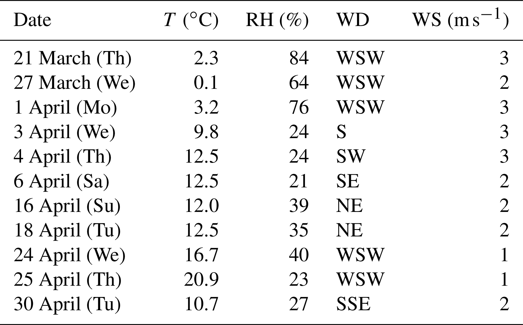
In Table A2 we collect the main characteristics of weather conditions for each measurement day. The weather information is provided for local noon from the observational data of the meteorological station located in the centre of St. Petersburg (index no. 26063, 59.97∘ N, 30.28∘ E). The daytime surface air temperature varied from ∼0 ∘C on 27 March to +21 ∘C on 25 April; relative humidity varied from 84 % on21 March to 21 % on 6 April. Generally, surface wind speed throughout the campaign was moderate in the range of 2–3 m s−1, except on 24 and 25 April, when light surface winds were recorded (1 m s−1). The prevailing winds for St. Petersburg are the southwesterly winds, and surface winds blowing from southwest and west-southwest were recorded during most days of the campaign; however, other wind directions were recorded, too (see Table A2). An average wind is calculated for the time period of FTIR observations. Resulting wind speeds and directions from the three different data sources are given in Table A3.
Table A2Basic meteorological data for the days of the field campaign: surface air temperature (T), relative humidity (RH), wind speed (WS) and wind direction (WD) at local noon. The meteorological data refer to one of the observational sites in the city of St. Petersburg (http://rp5.ru/Weather_archive_in_Saint_Petersburg, last access: 5 March 2020).
The satellite images of cloud cover detected by the MODIS satellite instrument in the vicinity of St. Petersburg are presented in Fig. A1. They confirm daytime clear-sky conditions for the duration of the campaign, except the day of 30 April, when altocumulus translucidus clouds started to develop.
Table A3The wind speed and the wind direction for the days of the field campaign, as retrieved from different data sources: in situ observations (LOCAL), globally gridded assimilated data (GDAS) and backward trajectory calculations (HYSPLIT).
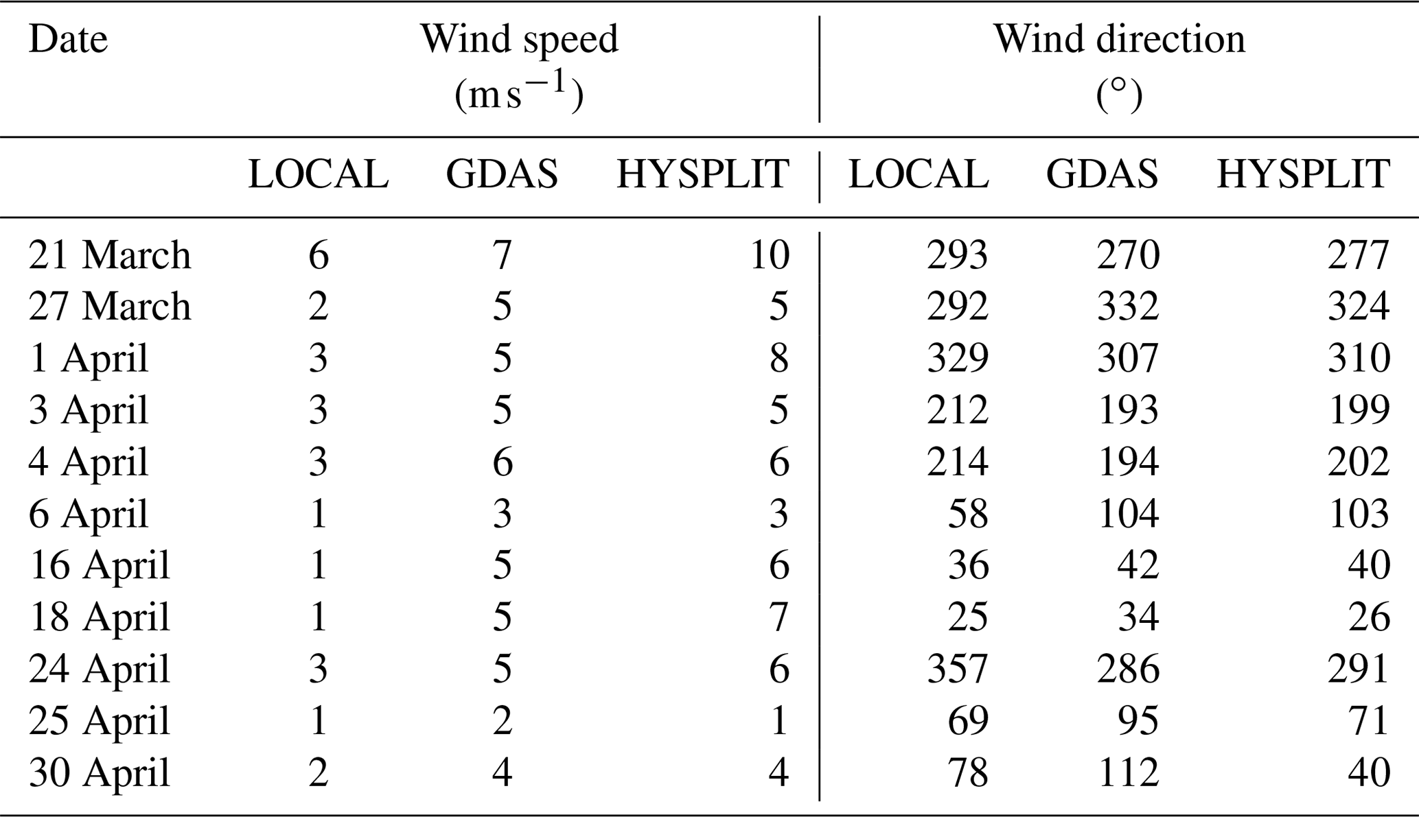
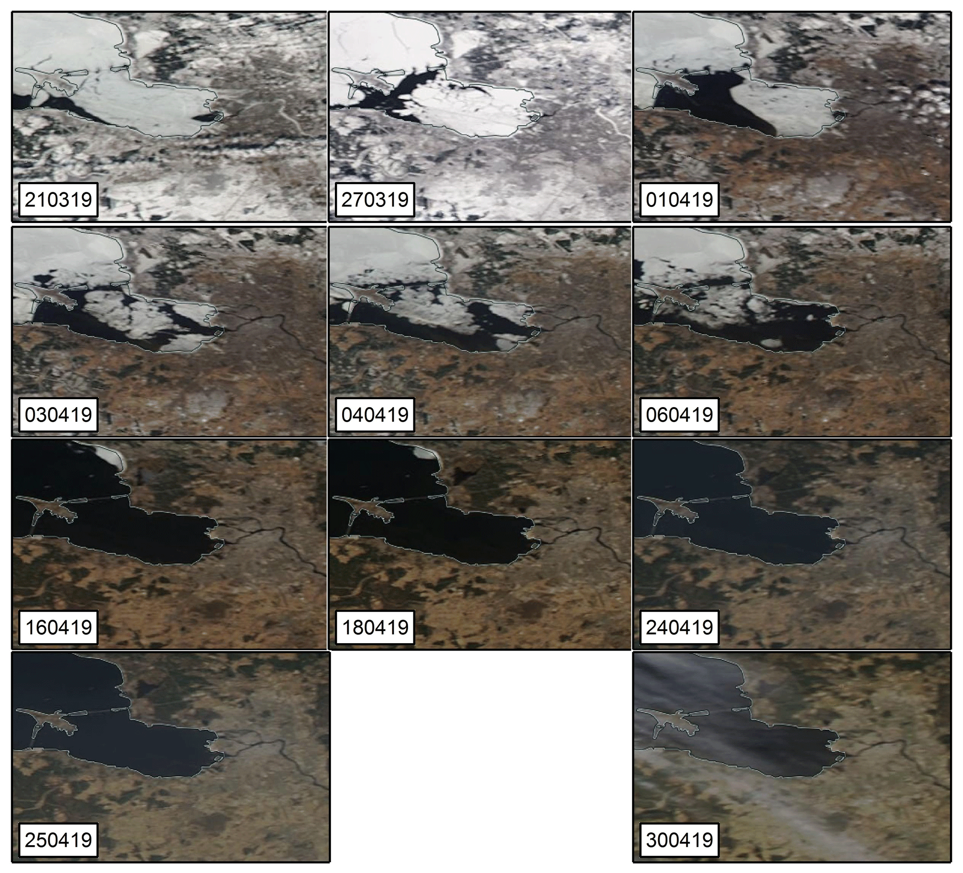
Figure A1The MODIS satellite images of cloud cover in the vicinity of St. Petersburg taken on the days of the field campaign.
Area fluxes for CO2, CH4, CO and NOx estimated using the simplified box model setup with a constant path length ( 27 km for each day of field observations) are given in Table B1.
Table B1Area fluxes for CO2 (), CH4 (), CO () and NOx () obtained using the constant path length approach.
We illustrate the transport of the pollutants from elevated sources with a HYSPLIT simulation (see Fig. C1). We selected one of the days of EMME (April 16, 2019) and simulated the CO2 emission from a 180 m chimney of the thermal power station mentioned above in the main text of the article. The plot presents a 34 h trajectory of the mass-weighted CO2 plume position (the centroid of the plume) on the geographical map (top panel) and using the altitude scale (bottom panel). One can see that the plume centroid starts its movement from the chimney location at ∼ 180 m altitude (12:00 of 15 April) and raises up to ∼ 500 m in 1 h; then it does not fall below the level of ∼ 350 m during its “flight” length of more than 300 km. The detailed analysis of respective vertical profiles of CO2 concentration shows its maximum at ∼ 500 m, being 1.2 times higher than that on the surface at the start and 3.6 times higher than that on the surface at the end of the plume trajectory. Thus, the probability of recording high concentrations corresponding to the centroid of the plume by surface-based observations can be estimated as being very low. Moreover, polluted air mass from a chimney is more likely to rise up rather than descend to the ground due to two reasons: (1) the vertical velocity of the air pollution jet emitted from a chimney can be rather high; (2) the temperature of a plume released from the chimney is usually significantly higher than the temperature of the ambient air, causing the buoyancy effect.
Elevated air sampling using kite launches was performed only twice during the EMME campaign; therefore the results of these kind of measurements could not be considered as a reliable confirmation of the absence of elevated plumes. The presence of the elevated plumes of CO and CO2 could also be confirmed by the following evidence. The comparison of the values of area fluxes (F; see Table 1) estimated using in situ measurements (column no. 4) and FTIR observations (column no. 2 and no. 3) shows that for CH4, of which sources are mainly located on the ground surface, we obtain a significantly lower difference in corresponding F values than for CO and CO2.
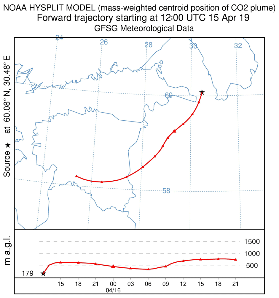
Figure C1Evolution of the mass-weighted centroid position of the CO2 plume taken as an example (see text).
The datasets containing the EM27/SUN measurements during EMME-2019 can be provided upon request; please contact Maria Makarova (m.makarova@spbu.ru) and Frank Hase (frank.hase@kit.edu).
MVM, FH, TB and DVI conceived the study together. MVM, DVI, YAV, CA, VSK, SCF, MF, TW, AnVP, KAV, NAZ, YMT, EYB, SIO, BKM, AlVP, EFM and HKhI contributed greatly to the experimental part of the study. SCF, CA and MVM were in charge of processing FTIR spectrometer data. DVI was in charge of the numerical modelling of gas plumes and of conducting the mobile DOAS measurements. Together MVM, FH, TB, DVI, SCF, CA, VSK, NNP and VMI analysed and interpreted the results. MVM, VSK, DVI and SCF prepared the original draft of the manuscript with contributions from FH, TB, CA, MF, YMT, NNP and VMI. MVM, FH, TB, DVI, VSK, MF, AlVP and YMT reviewed and edited the manuscript.
The authors declare that they have no conflict of interest.
Two portable EM27/SUN FTIR spectrometers were provided to St. Petersburg State University, Russia, by the owner, Karlsruhe Institute of Technology, Germany, in compliance with the conditions of temporary importation in the frame of the VERIFY project. The procedure of temporary importation of the instruments to the Russian Federation was conducted by the University of Bremen, Germany. Ancillary experimental data were acquired using the scientific equipment of the Research Center Geomodel of St. Petersburg State University. The authors gratefully acknowledge the NOAA ARL for the provision of the HYSPLIT transport and dispersion model and/or READY website (http://www.ready.noaa.gov, last access: 2 March 2020) used in this publication. The operation of the CIMEL sun photometer and Los Gatos Research GGA 24r-EP, Los Gatos Research CO 23r and ThermoScientific 42i-TL gas analysers was provided by the Research Center Geomodel of St. Petersburg State University (http://geomodel.spbu.ru/, last access: 2 March 2020).
This research has been supported by the European Commission, H2020 Observation-based system for monitoring and verification of greenhouse gases (VERIFY (grant no. 776810)) and the Russian Foundation for Basic Research (grant no. 18-05-00011).
The article processing charges for this open-access
publication were covered by a Research
Centre of the Helmholtz Association.
This paper was edited by Kimberly Strong and reviewed by two anonymous referees.
Ammoura, L., Xueref-Remy, I., Gros, V., Baudic, A., Bonsang, B., Petit, J.-E., Perrussel, O., Bonnaire, N., Sciare, J., and Chevallier, F.: Atmospheric measurements of ratios between CO2 and co-emitted species from traffic: a tunnel study in the Paris megacity, Atmos. Chem. Phys., 14, 12871–12882, https://doi.org/10.5194/acp-14-12871-2014, 2014.
Arya, S. P.: Air Pollution Meteorology and Dispersion, Oxford Univ. Press, New York, 310 pp., 1999.
Babenhauserheide, A., Hase, F., and Morino, I.: Net CO2 fossil fuel emissions of Tokyo estimated directly from measurements of the Tsukuba TCCON site and radiosondes, Atmos. Meas. Tech., 13, 2697–2710, https://doi.org/10.5194/amt-13-2697-2020, 2020.
Beran, D. W. and Hall Jr., F. F.: Remote sensing for air pollution meteorology, B. Am. Meteorol. Soc., 55, 1097–1105, 1974.
Bergamaschi, P., Karstens, U., Manning, A. J., Saunois, M., Tsuruta, A., Berchet, A., Vermeulen, A. T., Arnold, T., Janssens-Maenhout, G., Hammer, S., Levin, I., Schmidt, M., Ramonet, M., Lopez, M., Lavric, J., Aalto, T., Chen, H., Feist, D. G., Gerbig, C., Haszpra, L., Hermansen, O., Manca, G., Moncrieff, J., Meinhardt, F., Necki, J., Galkowski, M., O'Doherty, S., Paramonova, N., Scheeren, H. A., Steinbacher, M., and Dlugokencky, E.: Inverse modelling of European CH4 emissions during 2006–2012 using different inverse models and reassessed atmospheric observations, Atmos. Chem. Phys., 18, 901–920, https://doi.org/10.5194/acp-18-901-2018, 2018.
Cambaliza, M. O. L., Shepson, P. B., Caulton, D. R., Stirm, B., Samarov, D., Gurney, K. R., Turnbull, J., Davis, K. J., Possolo, A., Karion, A., Sweeney, C., Moser, B., Hendricks, A., Lauvaux, T., Mays, K., Whetstone, J., Huang, J., Razlivanov, I., Miles, N. L., and Richardson, S. J.: Assessment of uncertainties of an aircraft-based mass balance approach for quantifying urban greenhouse gas emissions, Atmos. Chem. Phys., 14, 9029–9050, https://doi.org/10.5194/acp-14-9029-2014, 2014.
Chen, J., Viatte, C., Hedelius, J. K., Jones, T., Franklin, J. E., Parker, H., Gottlieb, E. W., Wennberg, P. O., Dubey, M. K., and Wofsy, S. C.: Differential column measurements using compact solar-tracking spectrometers, Atmos. Chem. Phys., 16, 8479–8498, https://doi.org/10.5194/acp-16-8479-2016, 2016.
COCCON (COllaborative Carbon Column Observing Network): available at: http://www.imk-asf.kit.edu/english/COCCON.php, last access: 25 November 2019.
Crippa, M., Oreggioni, G., Guizzardi, D., Muntean, M., Schaaf, E., Lo Vullo, E., Solazzo, E., Monforti-Ferrario, F., Olivier, J. G. J., and Vignati, E.: Fossil CO2 and GHG emissions of all world countries – 2019 Report, EUR 29849 EN, Publications Office of the European Union, Luxembourg, ISBN 978-92-76-11100-9, JRC117610, https://doi.org/10.2760/687800, 2019.
de Foy, B., Lei, W., Zavala, M., Volkamer, R., Samuelsson, J., Mellqvist, J., Galle, B., Martínez, A.-P., Grutter, M., Retama, A., and Molina, L. T.: Modelling constraints on the emission inventory and on vertical dispersion for CO and SO2 in the Mexico City Metropolitan Area using Solar FTIR and zenith sky UV spectroscopy, Atmos. Chem. Phys., 7, 781–801, https://doi.org/10.5194/acp-7-781-2007, 2007.
Dlugokencky, E. J., Myers, R. C., Lang, P. M., Masarie, K. A., Crotwell, A. M., Thoning, K. W., Hall, B. D., Elkins, J. W., and Steele, L. P.: Conversion of NOAA atmospheric dry air CH4 mole fractions to a gravimetrically prepared standard scale, J. Geophys. Res., 110, D18306, https://doi.org/10.1029/2005JD006035, 2005.
Draxler, R. R. and Hess, G. D.: An overview of the HYSPLIT_4 modelling system for trajectories, dispersion, and deposition, Aust. Meteorol. Mag., 47, 295–308, 1998.
EDGAR (Emission Database for Global Atmospheric Research): available at: https://edgar.jrc.ec.europa.eu/overview.php?v=booklet2019&dst=CO2pc (last access: 21 November 2019), 2018.
ESRL (Earth System Research Laboratory) Global Monitoring Division: available at: https://www.esrl.noaa.gov/gmd/ccgg/ (last access: 12 November 2019), 2019.
Frey, M., Hase, F., Blumenstock, T., Groß, J., Kiel, M., Mengistu Tsidu, G., Schäfer, K., Sha, M. K., and Orphal, J.: Calibration and instrumental line shape characterization of a set of portable FTIR spectrometers for detecting greenhouse gas emissions, Atmos. Meas. Tech., 8, 3047–3057, https://doi.org/10.5194/amt-8-3047-2015, 2015.
Frey, M., Sha, M. K., Hase, F., Kiel, M., Blumenstock, T., Harig, R., Surawicz, G., Deutscher, N. M., Shiomi, K., Franklin, J. E., Bösch, H., Chen, J., Grutter, M., Ohyama, H., Sun, Y., Butz, A., Mengistu Tsidu, G., Ene, D., Wunch, D., Cao, Z., Garcia, O., Ramonet, M., Vogel, F., and Orphal, J.: Building the COllaborative Carbon Column Observing Network (COCCON): long-term stability and ensemble performance of the EM27/SUN Fourier transform spectrometer, Atmos. Meas. Tech., 12, 1513–1530, https://doi.org/10.5194/amt-12-1513-2019, 2019.
Gisi, M., Hase, F., Dohe, S., Blumenstock, T., Simon, A., and Keens, A.: XCO2-measurements with a tabletop FTS using solar absorption spectroscopy, Atmos. Meas. Tech., 5, 2969–2980, https://doi.org/10.5194/amt-5-2969-2012, 2012.
Hanna, S. R., Briggs, G. A., and Hosker, R. P.: Handbook on Atmospheric Diffusion, Department of Energy ReportDOE/TIC-11223, Washington, D.C., 102 pp., 1982.
Hase, F., Frey, M., Blumenstock, T., Groß, J., Kiel, M., Kohlhepp, R., Mengistu Tsidu, G., Schäfer, K., Sha, M. K., and Orphal, J.: Application of portable FTIR spectrometers for detecting greenhouse gas emissions of the major city Berlin, Atmos. Meas. Tech., 8, 3059–3068, https://doi.org/10.5194/amt-8-3059-2015, 2015.
Hase, F., Frey, M., Kiel, M., Blumenstock, T., Harig, R., Keens, A., and Orphal, J.: Addition of a channel for XCO observations to a portable FTIR spectrometer for greenhouse gas measurements, Atmos. Meas. Tech., 9, 2303–2313, https://doi.org/10.5194/amt-9-2303-2016, 2016.
Helfter, C., Famulari, D., Phillips, G. J., Barlow, J. F., Wood, C. R., Grimmond, C. S. B., and Nemitz, E.: Controls of carbon dioxide concentrations and fluxes above central London, Atmos. Chem. Phys., 11, 1913–1928, https://doi.org/10.5194/acp-11-1913-2011, 2011.
Hiller, R. V., Neininger, B., Brunner, D., Gerbig, C., Bretscher, D., Künzle, T., Buchmann, N., and Eugster, W.: Aircraft-based CH4 flux estimates for validation of emissions from an agriculturally dominated area in Switzerland, J. Geophys. Res.-Atmos., 119, 4874–4887, https://doi.org/10.1002/2013JD020918, 2014a.
Hiller, R. V., Bretscher, D., DelSontro, T., Diem, T., Eugster, W., Henneberger, R., Hobi, S., Hodson, E., Imer, D., Kreuzer, M., Künzle, T., Merbold, L., Niklaus, P. A., Rihm, B., Schellenberger, A., Schroth, M. H., Schubert, C. J., Siegrist, H., Stieger, J., Buchmann, N., and Brunner, D.: Anthropogenic and natural methane fluxes in Switzerland synthesized within a spatially explicit inventory, Biogeosciences, 11, 1941–1959, https://doi.org/10.5194/bg-11-1941-2014, 2014b.
Ibrahim, O., Shaiganfar, R., Sinreich, R., Stein, T., Platt, U., and Wagner, T.: Car MAX-DOAS measurements around entire cities: quantification of NOx emissions from the cities of Mannheim and Ludwigshafen (Germany), Atmos. Meas. Tech., 3, 709–721, https://doi.org/10.5194/amt-3-709-2010, 2010.
ICOS (Integrated Carbon Observation System): available at: https://www.icos-ri.eu, last access: 2 March 2020.
Ionov, D. V. and Poberovskii, A. V.: Nitrogen dioxide in the air basin of St. Petersburg: Remote measurements and numerical simulation, Izv. Atmos. Ocean. Phys.+, 48, 373–383, https://doi.org/10.1134/S0001433812040093, 2012.
Ionov, D. V. and Poberovskii, A. V.: Quantification of NOx emission from St. Petersburg (Russia) using mobile DOAS measurements around entire city, Int. J. Remote Sens., 36, 2486–2502, https://doi.org/10.1080/01431161.2015.1042123, 2015.
Ionov, D. V. and Poberovskii A. V.: Integral emission of nitrogen oxides from the territory of St. Petersburg based on the data of mobile measurements and numerical simulation results, Izv. Atmos. Ocean. Phys.+, 53, 204–212, https://doi.org/10.1134/S0001433817020049, 2017.
Ionov, D. V. and Poberovskii A. V.: Observations of urban NOx plume dispersion using the mobile and satellite DOAS measurements around the megacity of St. Petersburg (Russia), Int. J. Remote Sens., 40, 719–733, https://doi.org/10.1080/01431161.2018.1519274, 2019.
IPCC: Climate Change 2013: The Physical Science Basis. Contribution of Working Group I to the Fifth Assessment Report of the Intergovernmental Panel on Climate Change, Cambridge University Press, Cambridge, UK and New York, NY, USA, https://doi.org/10.1017/CBO9781107415324, 2013.
Johansson, J. K. E., Mellqvist, J., Samuelsson, J., Offerle, B., Lefer, B., Rappenglück, B., Flynn, J., and Yarwood, G.: Emission measurements of alkenes, alkanes, SO2, and NO2 from stationary sources in Southeast Texas over a 5 year period using SOF and mobile DOAS, J. Geophys. Res.-Atmos., 119, 1973–1991, https://doi.org/10.1002/2013JD020485, 2014.
Johansson, M., Galle, B., Yu, T., Tang, L., Chen, D., Li, H., Li, J. X., and Zhang, Y.: Quantification of total emission of air pollutants from Beijing using mobile mini-DOAS, Atmos. Environ., 42, 6926–6933, 2008.
Johansson, M., Rivera, C., de Foy, B., Lei, W., Song, J., Zhang, Y., Galle, B., and Molina, L.: Mobile mini-DOAS measurement of the outflow of NO2 and HCHO from Mexico City, Atmos. Chem. Phys., 9, 5647–5653, https://doi.org/10.5194/acp-9-5647-2009, 2009.
Keppel-Aleks, G., Toon, G. C., Wennberg, P. O., and Deutscher, N. M.: Reducing the impact of source brightness fluctuations on spectra obtained by Fourier-transform spectrometry, Appl. Optics, 46, 4774–4779, 2007.
Kille, N., Baidar, S., Handley, P., Ortega, I., Sinreich, R., Cooper, O. R., Hase, F., Hannigan, J. W., Pfister, G., and Volkamer, R.: The CU mobile Solar Occultation Flux instrument: structure functions and emission rates of NH3, NO2 and C2H6, Atmos. Meas. Tech., 10, 373–392, https://doi.org/10.5194/amt-10-373-2017, 2017.
Kostsov, V. S.: Retrieving Cloudy Atmosphere Parameters from RPG-HATPRO Radiometer Data, Izv. Atmos. Ocean. Phys.+, 51, 156–166, https://doi.org/10.1134/S0001433815020085, 2015.
Kostsov, V. S., Ionov, D. V., Biryukov, E. Yu., and Zaitsev, N. A.: Cross-validation of two liquid water path retrieval algorithms applied to ground-based microwave radiation measurements by the RPG-HATPRO instrument, Int. J. Remote Sens., 39, 1–22, https://doi.org/10.1080/01431161.2017.1404163, 2018.
Lee, J. D., Helfter, C., Purvis, R. M., Beevers, S. D., Carslaw, D. C., Lewis, A. C., Møller, S. J., Tremper, A., Vaughan, A., and Nemitz, E. G.: Measurement of NOx Fluxes from a Tall Tower in Central London, UK and Comparison with Emissions Inventories, Environ. Sci. Technol., 49, 1025–1034, https://doi.org/10.1021/es5049072, 2015.
Lopez, M., Schmidt, M., Ramonet, M., Bonne, J.-L., Colomb, A., Kazan, V., Laj, P., and Pichon, J.-M.: Three years of semicontinuous greenhouse gas measurements at the Puy de Dôme station (central France), Atmos. Meas. Tech., 8, 3941–3958, https://doi.org/10.5194/amt-8-3941-2015, 2015.
Luther, A., Kleinschek, R., Scheidweiler, L., Defratyka, S., Stanisavljevic, M., Forstmaier, A., Dandocsi, A., Wolff, S., Dubravica, D., Wildmann, N., Kostinek, J., Jöckel, P., Nickl, A.-L., Klausner, T., Hase, F., Frey, M., Chen, J., Dietrich, F., Nȩcki, J., Swolkień, J., Fix, A., Roiger, A., and Butz, A.: Quantifying CH4 emissions from hard coal mines using mobile sun-viewing Fourier transform spectrometry, Atmos. Meas. Tech., 12, 5217–5230, https://doi.org/10.5194/amt-12-5217-2019, 2019.
Makarova, M. V., Poberovskii, A. V., Yagovkina, S. V., Karol', I. L., Lagun, V. E., Paramonova, N. N., Reshetnikov, A. I., and Privalov, V. I.: Study of the formation of the methane field in the atmosphere over northwestern Russia, Izv. Atmos. Ocean. Phys.+, 42, 215–227, https://doi.org/10.1134/S0001433806020083, 2006.
Makarova, M. V., Rakitin, A. V., Ionov, D. V., and Poberovskii A. V.: Analysis of variability of the CO, NO2, and O3 contents in the troposphere near St. Petersburg, Izv. Atmos. Ocean. Phys.+, 47, 508–520, https://doi.org/10.1134/S0001433811040074, 2011.
Makarova, M. V., Arabadzhyan, D. K., Foka, S. C., Paramonova, N. N., Poberovskii, A. V., Timofeev, Yu. M., Pankratova, N. V., and Rakitin, V. S.: Estimation of Nocturnal Area Fluxes of Carbon Cycle Gases in Saint Petersburg Suburbs, Russ. Meteorol. Hydrol., 43, 449–455, https://doi.org/10.3103/S106837391807004X, 2018.
Maksyutov, S., Takagi, H., Valsala, V. K., Saito, M., Oda, T., Saeki, T., Belikov, D. A., Saito, R., Ito, A., Yoshida, Y., Morino, I., Uchino, O., Andres, R. J., and Yokota, T.: Regional CO2 flux estimates for 2009–2010 based on GOSAT and ground-based CO2 observations, Atmos. Chem. Phys., 13, 9351–9373, https://doi.org/10.5194/acp-13-9351-2013, 2013.
Marr, L. C., Moore, T. O., Klapmeyer, M. E., and Killar, M. B.: Comparison of NOx fluxes measured by eddy covariance to emission inventories and land use, Environ. Sci. Technol., 47, 1800–1808, https://doi.org/10.1021/es303150y, 2013.
Mellqvist, J., Samuelsson, J., Johansson, J., Rivera, C., Lefer, B., Alvarez, S., and Jolly, J.: Measurements of industrial emissions of alkenes in Texas using the solar occultation flux method, J. Geophys. Res., 115, D00F17, https://doi.org/10.1029/2008JD011682, 2010.
Moriwaki, R. and Kanda, M.: Seasonal and diurnal fluxes of radia-tion, heat, water vapor, and carbon dioxide over a suburban area, J. Appl. Meteorol., 43, 1700–1710, https://doi.org/10.1175/JAM2153.1, 2004.
NDACC (Network for the Detection of Atmospheric Composition Change): available at: http://www.ndaccdemo.org/, last access: 12 November 2019.
O'Shea, S. J., Allen, G., Fleming, Z. L., Bauguitte, S. J.-B., Percival, C. J., Gallagher, M. W., Lee, J., Helfter C., and Nemitz E.:. Area fluxes of carbon dioxide, methane, and carbon monoxide derived from airborne measurements around Greater London: A case study during summer 2012, J. Geophys. Res.-Atmos., 119, 4940–4952, https://doi.org/10.1002/2013JD021269, 2014.
Platt, U. and Stutz, J.: Differential Optical Absorption Spectroscopy (DOAS), Principles and Applications, Springer, Berlin-Heidelberg, 598 pp., https://doi.org/10.1007/978-3-540-75776-4, ISBN 978-3-540-21193-8, 2008.
Reid, K. H. and Steyn, D. G.: Diurnal variations of boundary-layer carbon dioxide in a coastal city–Observations and comparison with model results, Atmos. Environ., 31, 3101–3114, https://doi.org/10.1016/S1352-2310(97)00050-2, 1997.
Rivera, C., Sosa, G., Wöhrnschimmel, H., de Foy, B., Johansson, M., and Galle, B.: Tula industrial complex (Mexico) emissions of SO2 and NO2 during the MCMA 2006 field campaign using a mobile mini-DOAS system, Atmos. Chem. Phys., 9, 6351–6361, https://doi.org/10.5194/acp-9-6351-2009, 2009.
Rivera, C., Mellqvist, J., Samuelsson, J., Lefer, B., Alvarez, S., and Patel, M. R.: Quantification of NO2 and SO2 emissions from the Houston Ship Channel and Texas City industrial areas during the 2006 Texas Air Quality Study, J. Geophys. Res., 115, D08301, https://doi.org/10.1029/2009JD012675, 2010.
Schmidt, M., Lopez, M., Yver Kwok, C., Messager, C., Ramonet, M., Wastine, B., Vuillemin, C., Truong, F., Gal, B., Parmentier, E., Cloué, O., and Ciais, P.: High-precision quasi-continuous atmospheric greenhouse gas measurements at Trainou tower (Orléans forest, France), Atmos. Meas. Tech., 7, 2283–2296, https://doi.org/10.5194/amt-7-2283-2014, 2014.
Serebritsky, I. A. (Ed.): The Report on Environmental Conditions in St. Petersburg for 2017, available at: https://www.gov.spb.ru/static/writable/ckeditor/uploads/2018/06/29/Doklad_EKOLOGIA2018.pdf (last access: 2 March 2020), 2018 (in Russian).
Serebritsky, I. A. (Ed.): The Report on Environmental Conditions in St. Petersburg for 2018, available at: https://www.gov.spb.ru/static/writable/ckeditor/uploads/2019/08/12/42/doklad_za_2018_EKOLOGIA2019.pdf (last access: 2 March 2020), 2019 (in Russian).
Shaiganfar, R., Beirle, S., Sharma, M., Chauhan, A., Singh, R. P., and Wagner, T.: Estimation of NOx emissions from Delhi using Car MAX-DOAS observations and comparison with OMI satellite data, Atmos. Chem. Phys., 11, 10871–10887, https://doi.org/10.5194/acp-11-10871-2011, 2011.
Shaiganfar, R., Beirle, S., Petetin, H., Zhang, Q., Beekmann, M., and Wagner, T.: New concepts for the comparison of tropospheric NO2 column densities derived from car-MAX-DOAS observations, OMI satellite observations and the regional model CHIMERE during two MEGAPOLI campaigns in Paris 2009/10, Atmos. Meas. Tech., 8, 2827–2852, https://doi.org/10.5194/amt-8-2827-2015, 2015.
Shaiganfar, R., Beirle, S., Denier van der Gon, H., Jonkers, S., Kuenen, J., Petetin, H., Zhang, Q., Beekmann, M., and Wagner, T.: Estimation of the Paris NOx emissions from mobile MAX-DOAS observations and CHIMERE model simulations during the MEGAPOLI campaign using the closed integral method, Atmos. Chem. Phys., 17, 7853–7890, https://doi.org/10.5194/acp-17-7853-2017, 2017.
Stein, A. F., Isakov, V., Godowitch, J., and Draxler, R. R.: A hybrid modeling approach to resolve pollutant concentrations in an urban area, Atmos. Environ., 41, 9410–9426, https://doi.org/10.1016/j.atmosenv.2007.09.004, 2007.
Stein, A. F., Draxler, R. R., Rolph, G. D., Stunder, B. J. B., and Cohen, M. D., and Ngan F.: NOAA's HYSPLIT atmospheric transport and dispersion modeling system, B. Am. Meteorol. Soc., 96, 2059–2077, https://doi.org/10.1175/BAMS-D-14-00110.1, 2015.
Stremme, W., Grutter, M., Rivera, C., Bezanilla, A., Garcia, A. R., Ortega, I., George, M., Clerbaux, C., Coheur, P.-F., Hurtmans, D., Hannigan, J. W., and Coffey, M. T.: Top-down estimation of carbon monoxide emissions from the Mexico Megacity based on FTIR measurements from ground and space, Atmos. Chem. Phys., 13, 1357–1376, https://doi.org/10.5194/acp-13-1357-2013, 2013.
Strong, C., Stwertka, C., Bowling, D. R., Stephens, B. B., and Ehleringer J. R.: Urban carbon dioxide cycles within the Salt Lake Valley: A multiple-box model validated by observations, J. Geophys. Res., 116, D15307, https://doi.org/10.1029/2011JD015693, 2011.
TCCON: Total Carbon Column Observing Network, available at: http://tccon.caltech.edu/, last access: 12 November 2019.
Turnbull, J. C., Karion, A., Fischer, M. L., Faloona, I., Guilderson, T., Lehman, S. J., Miller, B. R., Miller, J. B., Montzka, S., Sherwood, T., Saripalli, S., Sweeney, C., and Tans, P. P.: Assessment of fossil fuel carbon dioxide and other anthropogenic trace gas emissions from airborne measurements over Sacramento, California in spring 2009, Atmos. Chem. Phys., 11, 705–721, https://doi.org/10.5194/acp-11-705-2011, 2011.
Turnbull, J. C., Sweeney, C., Karion, A., Newberger, T., Lehman, S. J., Cambaliza, M. O., Shepson, P. B., Gurney, K., Patarasuk, R., and Razlivanov, I.: Toward quantification and source sector identification of fossil fuel CO2 emissions from an urban area: Results from the INFLUX experiment, J. Geophys. Res.-Atmos., 120, 292–312, https://doi.org/10.1002/2014JD022555, 2015.
Turner, A. J., Jacob, D. J., Wecht, K. J., Maasakkers, J. D., Lundgren, E., Andrews, A. E., Biraud, S. C., Boesch, H., Bowman, K. W., Deutscher, N. M., Dubey, M. K., Griffith, D. W. T., Hase, F., Kuze, A., Notholt, J., Ohyama, H., Parker, R., Payne, V. H., Sussmann, R., Sweeney, C., Velazco, V. A., Warneke, T., Wennberg, P. O., and Wunch, D.: Estimating global and North American methane emissions with high spatial resolution using GOSAT satellite data, Atmos. Chem. Phys., 15, 7049–7069, https://doi.org/10.5194/acp-15-7049-2015, 2015.
Vaughan, A. R., Lee, J. D., Misztal, P. K., Metzger, S., Shaw, M. D., Lewis, A. C., Purvis, R. M., Carslaw, D. C., Goldstein, A. H., Hewitt, C. N., Davison, B., Beevers, S. D., and Karl, T. G.: Spatially resolved flux measurements of NOx from London suggest significantly higher emissions than predicted by inventories, Faraday Discuss., 189, 455–472, https://doi.org/10.1039/C5FD00170F, 2016.
Velasco, E., Pressley, S., Allwine, E., Westberg, H., and Lamb, B.: Measurements of CO2 fluxes from the Mexico City urban land-scape, Atmos. Environ., 39, 7433–7446, https://doi.org/10.1016/j.atmosenv.2005.08.038, 2005.
VERIFY – VERIFYING GREENHOUSE GAS EMISSIONS: available at: https://verify.lsce.ipsl.fr/, last access: 12 November 2019.
Viatte, C., Lauvaux, T., Hedelius, J. K., Parker, H., Chen, J., Jones, T., Franklin, J. E., Deng, A. J., Gaudet, B., Verhulst, K., Duren, R., Wunch, D., Roehl, C., Dubey, M. K., Wofsy, S., and Wennberg, P. O.: Methane emissions from dairies in the Los Angeles Basin, Atmos. Chem. Phys., 17, 7509–7528, https://doi.org/10.5194/acp-17-7509-2017, 2017.
Vogel, F. R., Frey, M., Staufer, J., Hase, F., Broquet, G., Xueref-Remy, I., Chevallier, F., Ciais, P., Sha, M. K., Chelin, P., Jeseck, P., Janssen, C., Té, Y., Groß, J., Blumenstock, T., Tu, Q., and Orphal, J.: XCO2 in an emission hot-spot region: the COCCON Paris campaign 2015, Atmos. Chem. Phys., 19, 3271–3285, https://doi.org/10.5194/acp-19-3271-2019, 2019.
Volkova, K. A., Poberovsky, A. V., Timofeev, Yu. M., Ionov, D. V., Holben, B. N., Smirnov, A., and Slutsker, I.: Aerosol Optical Characteristics Retrieved from CIMEL Sun Photometer Measurements (AERONET) near St. Petersburg, Atmos. Ocean Opt., 31, 635–641, https://doi.org/10.1134/S1024856018060180, 2018.
Wang, S., Zhou, B., Wang, Z., Yang, S., Hao, N., Valks, P., Trautmann, T., and Chen, L.: Remote sensing of NO2 emission from the central urban area of Shanghai (China) using the mobile DOAS technique, J. Geophys. Res., 117, D13305, https://doi.org/10.1029/2011JD016983, 2012.
WMO: Guidelines for the Measurement of Methane and Nitrous Oxide and their Quality Assurance, WMO TD No. 1478, 49 p., 2009.
WMO: 17th WMO/IAEA Meeting on Carbon Dioxide, Other Greenhouse Gases, and Related Measurement Techniques (GGMT-2013), Beijing, China, 10–13 June 2013, 158 p., 2014.
WMO: Greenhouse Gas Bulletin, 22 November 2018, 14, 1–8, available at: https://library.wmo.int/doc_num.php?explnum_id=5455 (last access 2 March 2020), 2018.
Wu, F., Li, A., Xie, P., Chen, H., Hu, Z., Zhang, Q., Liu, J., and Liu, W.: Emission flux measurement error with a mobile DOAS system and application to NOx flux observations, Sensors, 17, 231, https://doi.org/10.3390/s17020231, 2017.
Wunch, D., Wennberg, P. O., Toon, G. C., Keppel-Aleks, G., and Yavin, Y. G.: Emissions of greenhouse gases from a North American megacity, Geophys. Res. Lett., 36, L15810, https://doi.org/10.1029/2009GL039825, 2009.
Wunch, D., Toon, G. C., Blavier, J. F., Washenfelder, R. A., Notholt, J., Connor, B. J., Griffith, D. W., Sherlock, V., and Wennberg, P. O.: The total carbon column observing network, Philos. T. R. Soc. A, 369, 2087–112, https://doi.org/10.1098/rsta.2010.0240, 2011.
Zhao, X., Marshall, J., Hachinger, S., Gerbig, C., Frey, M., Hase, F., and Chen, J.: Analysis of total column CO2 and CH4 measurements in Berlin with WRF-GHG, Atmos. Chem. Phys., 19, 11279–11302, https://doi.org/10.5194/acp-19-11279-2019, 2019.
Zinchenko, A. V., Paramonova, N. N., Privalov, V. I., and Reshetnikov, A. I.: Estimation of methane emissions in the St. Petersburg, Russia, region: An atmospheric nocturnal boundary layer budget approach, J. Geophys. Res., 107, 4416, https://doi.org/10.1029/2001JD001369, 2002.
Zimnoch, M., Godlowska, J., Necki, J. M., and Rozanski, K.: Assessing surface fluxes of CO2 and CH4 in urban environment: a reconnaissance study in Krakow, Southern Poland, Tellus B, 62, 573–580, https://doi.org/10.1111/j.1600-0889.2010.00489.x, 2010.
- Abstract
- Introduction
- Concept of EMME, instruments and the experiment planning
- Overview of the 2019 campaign
- Methods and algorithms of the experimental data processing
- Results and discussion
- Summary and outlook
- Appendix A: Description of the experiment details and meteorological conditions
- Appendix B: Area fluxes for simplified box model setup
- Appendix C: Comments on transport of the pollutants from elevated sources
- Data availability
- Author contributions
- Competing interests
- Acknowledgements
- Financial support
- Review statement
- References