the Creative Commons Attribution 4.0 License.
the Creative Commons Attribution 4.0 License.
 | 10 Feb 2021
Hydrometeor classification of quasi-vertical profiles of polarimetric radar measurements using a top-down iterative hierarchical clustering method
David Dufton
Jonathan Crosier
Joshua M. Hampton
Lindsay Bennett
Ryan R. Neely III
Correct, timely and meaningful interpretation of polarimetric weather radar observations requires an accurate understanding of hydrometeors and their associated microphysical processes along with well-developed techniques that automatize their recognition in both the spatial and temporal dimensions of the data. This study presents a novel technique for identifying different types of hydrometeors from quasi-vertical profiles (QVPs). In this new technique, the hydrometeor types are identified as clusters belonging to a hierarchical structure. The number of different hydrometeor types in the data is not predefined, and the method obtains the optimal number of clusters through a recursive process. The optimal clustering is then used to label the original data. Initial results using observations from the National Centre for Atmospheric Science (NCAS) X-band dual-polarization Doppler weather radar (NXPol) show that the technique provides stable and consistent results. Comparison with available airborne in situ measurements also indicates the value of this novel method for providing a physical delineation of radar observations. Although this demonstration uses NXPol data, the technique is generally applicable to similar multivariate data from other radar observations.
- Article
(7333 KB) - Full-text XML
- BibTeX
- EndNote


The task of radar-based hydrometeor classification (HC) can be broadly defined as the recognition of different hydrometeor types in the atmosphere as represented by the various observed moments collected by weather radar. In general, HC is able to label radar signatures observed at any one time with physical properties, and, over a period of time, the evolution of these labels can provide insight into the underlying atmospheric processes. As such HC has many impactful applications: HC simplifies the detection of the melting layer (Baldini and Gorgucci, 2006), HC is necessary for obtaining accurate estimates of precipitation quantities (Giangrande and Ryzhkov, 2008) and HC provides critical information for improving modelling of physical processes in the atmosphere (Vivekanandan et al., 1999).
Radar-based HC requires an extensive and accurate (i.e. expert) knowledge of the physical properties of both multivariate polarimetric observations and the hydrometeor particles themselves (Hall et al., 1984). Achieving an accurate and precise radar-based HC is difficult due to the deficiencies (such as low spatial–temporal resolution) and inaccuracies (such as attenuation) that are inevitable in all radar measurements. The process of HC is made even more difficult when this analysis needs to be performed during the operational processing of the radar observations where there is a lack of time for expert assessment. Therefore, automatization of spatial and temporal analysis of multivariate polarimetric data is an important task for which an advanced and well-tested technique should be developed and utilized.
The development of radar-based HC started in the 1980s and 1990s with the works of Hall et al. (1984), Hendry and Antar (1984), Aydin et al. (1986), Straka and Zrnić (1993), and Straka (1996). Further refinement and development of automatic HC algorithms included the application of fuzzy logic (Straka et al., 2000; Liu and Chandrasekar, 2000), machine-learning techniques (such as the identification of clusters representing data-wise similarities) (Wen et al., 2015; Grazioli et al., 2015; Besic et al., 2016; Ribaud et al., 2019) and neural networks (Wang et al., 2017).
Modern radar-based HC methods (Straka et al, 1996; Liu and Chandrasekar, 2000; Al-Sakka et al., 2013; Grazioli et al., 2015; Besic et al., 2016, 2018; Bechini and Chandrasekar, 2015; Wang et al., 2017) are based on the multivariate data of polarimetric Doppler radar observations. This includes (but is not limited to) the horizontal reflectivity factor ZH, differential reflectivity ZDR, the co-polar correlation coefficient ρHV, differential phase shift on propagation ΦDP, and specific differential phase KDP (for definitions, see Bringi and Chandrasekar, 2001) as well as associated derived variables (e.g. standard deviation). Additionally, temperature and other meteorological data, retrieved from radiosondes or numerical weather prediction (NWP) models, are often utilized (Grazioli et al., 2015; Wen et al., 2015).
In most existing radar-based HC methods, the multivariate input data are analysed per measurement voxel, and determined classes are assigned to the hydrometeor types only according to their characteristics. Such an approach neglects intra-class relationships and the temporal evolution of the identified classes. This valuable information can also be used in the labelling of the hydrometeor types and the identification of corresponding microphysical processes. Additionally, almost all methods within the existing literature are based on theoretical assumptions on the scattering properties of observed particles and/or are only applicable for a defined (i.e. previously recognized) number and type of classes. Both of these aspects of existing HC methods are limitations. For example, theoretical assumptions about the scattering properties of ice-phase hydrometeors are very uncertain due to unknown size distributions, varying dielectric properties, fall orientation, and their diverse and often complex geometry (Johnson et al., 2012). A predefined number of classes or hydrometeor types is subjective and creates artificial boundaries for algorithms; therefore, subtle differences in undefined sub-classes are masked, which inhibits identification of the underlying microphysical processes.
Thus, in this study we take a different approach and ask the following question: can a data-driven HC approach provide an optimal number of classes from the observations? We define the optimal number as the lowest number of classes representing all pronounced dissimilarities in the input data. Once the optimal set of classes is identified, the burden of analysis in this approach is to relate the identified clusters of radar signatures to possible physical properties of hydrometeors. Thus, this approach does not impose a predefined physical view on the observations but provides a framework for a more efficient physical interpretation of the properties of the resulting clusters of observed multivariate data in which subtle differences and intra-cluster relations are easier to identify. In this sense, this approach inverts the procedure of existing methods. Additionally, we ask whether such an approach can be used to provide information on the temporal evolution of the identified hydrometeors and reveal relationships between the identified classes. Such information is key for identifying the processes that lead to high-impact weather (i.e. flooding) and improving the physical parameterizations in NWP.
The point of this study is not to create a set of cluster characteristics that could be applied to other datasets; rather, the goal is to demonstrate the viability of this type of data-driven methodology for creating a set of labelled clusters (i.e. hydrometeor classes) based on quasi-vertical profile (QVP) data. As such, the comparison to in situ data and labelling done as part of this study is only shown as an example of how this tool can be used.
The existing data-driven unsupervised (Grazioli et al., 2015; Ribaud et al., 2019; Tiira and Moisseev, 2020) and semi-supervised approaches (Bechini and Chandrasekar, 2015; Besic et al., 2016; Wang et al., 2017; Roberto et al., 2017; Besic et al., 2018) only partially provide an answer to the first question (Grazioli et al., 2015) and do not consider the temporal evolution or dependencies between the identified classes. The approach described here performs an unsupervised clustering of QVPs. QVPs were first used in Kumjian et al. (2013) and Ryzhkov et al. (2016) as a way of constructing a substitute for a vertical profile from a scan conducted at constant elevation, which is a typical mode of scanning for radars used in operational networks. Calculation of the QVPs requires horizontal homogeneity of the observed atmospheric processes. The height vs. time format of QVPs represents the general structure of the storm or its evolution. Note that this is a novel application of the QVP data product and the interpretation of QVP polarimetric variables differs from that of plan position indicator (PPI) or range height indicator (RHI) scans due to the averaging used to construct them.
The QVP input is used in this work to build a hierarchical structure based on the identified clusters and deliver an optimal number of clusters based solely on internal properties of the multivariate polarimetric data. The optimal clustering is then used to label the hydrometeor classes and to analyse the temporal evolution of the labelled microphysical processes.
The paper is organized as follows: in Sect. 2, we introduce the clustering methods we employ, Sect. 3 contains a description of the polarimetric radar data and their processing, Sect. 4 describes the iterative clustering approach, leading to the development of the hierarchical structure, Sect. 5 is devoted to the characterization of the clusters and their labelling, and Sect. 6 concludes with a summary, discussion, and thoughts on further perspectives.
The proposed hierarchical clustering algorithm identifies the optimal number of groups of data points (clusters) in a recursive loop and organizes the clusters in a hierarchical structure (undirected weighted graph). The two main steps of this approach are the cluster identification and the optimality check. The cluster identification is achieved after performing dimensionality reduction by principal component analysis followed by spectral clustering. The optimality check uses validity indexes to identify the final set of clusters, which best classifies the provided set of data. The description of the dimensionality reduction and clustering methods with background information about the validity indexes employed can be found in this section directly after a short introduction to the hierarchical clustering.
2.1 Hierarchical clustering
Hierarchical clustering is a type of clustering technique that splits or combines the data through an iterative process. Unlike “flat” clustering techniques, hierarchical clustering is not performed in one stage; rather, it repeats the clustering process iteratively and keeps the information about each iteration of clustering in a hierarchical structure. In general, for a given set of multivariate data points, a hierarchical clustering algorithm, depending on top-down or bottom-up direction, either partitions (divides) or merges (agglomerates) the data into groups (a set of clusters) where data points assigned to the same cluster show similarity in multivariate values (depending on the context, it could be, for example, having a small distance to each other if the points are in Euclidean space). The direction of the process (top-down or bottom-up) may be chosen and depends on the number of individual points in the multivariate dataset and the requirements of the underlying problem.
The top-down method begins with all available data points organized in one cluster and splits this cluster into sub-clusters until a certain criterion is reached or only solely singleton clusters of individual points remain in the set. The bottom-up method, on the other hand, begins with all points assigned to individual clusters and, at each step, merges the most similar pairs of clusters into one until all the sub-clusters are agglomerated into a single cluster.
The optimal number of clusters in both approaches can be identified using a termination criterion. The hierarchical structure in the bottom-up approach needs to be completely finished before the optimal number of clusters can be identified, otherwise the upper part of the tree will remain unknown. The top-down approach allows for the iterative process to be stopped at any point whilst preserving the upper part of the hierarchical structure. Another advantage of the top-down approach is the possibility to have more than two sub-clusters belonging to one parent cluster. This allows an optimal number of sub-clusters for each parent cluster, representing the data-driven inheritances in the resulting hierarchical structure. Although this advantage is often not used, and the bottom-up methods are preferred (Grazioli et al., 2015; Rimbaud et al., 2019), the method presented here fully exploits it for the identification of an optimal number of sub-clusters in each iteration.
2.2 Eigenvectors and principal components
Principal component analysis (PCA) is a statistical technique mostly utilized in exploratory analysis of multivariate data. It extracts the most important information from the multivariate dataset, generating a simplified view of the original data by dimensionality reduction.
To reduce a dataset's dimensionality, a set of new orthogonal, non-correlated variables called principal components is calculated as linear combinations of the original variables. The first component with the largest possible variance is selected, so it best represents the diversity of the given data. The second component is generated under the assumption of orthogonality to the first component whilst also having the largest possible variance. This process is continued until the number of principal components is equal to the number of original variables (d). These components are exactly the eigenvectors of the correlation matrix and are employed as a basis for a new coordinate system (Wold, 1976; Abdi and Williams, 2010). The first q calculated coordinates having satisfactory representativeness (e.g. 85 %) can be used to preserve the most important characteristics of the original data. These q principal components can replace the initial d variables (q<d), and the original dataset, consisting of N measurements on d variables, is reduced to a dataset consisting of N measurements on q principal components.
2.3 Clustering method
One of the most popular clustering methods is the k-means algorithm (Steinhaus, 1956). Through its simple interpretability, it is often used either as a single method or as a part of more computationally expensive clustering methods (e.g. Gaussian mixtures or spectral clustering). As a single method, it has difficulties with non-convex clusters and is known to perform poorly if the input variables are correlated (von Luxburg, 2007). As the basis of a more complex method (e.g. spectral clustering), it allows a solution of non-linear cluster shapes to be found (any low-dimensional manifolds of high-dimensional spaces).
The input data herein are multidimensional and were found to have non-convex cluster shapes; therefore, the spectral clustering method was applied (Shi and Malik, 2000; Ng et al., 2002; von Luxburg, 2007). It works by approximating the problem of partitioning the nodes in a weighted graph as an eigenvalue problem of eigenvectors described above and by applying the k-means algorithm to this representation in order to obtain the clusters. This work implements the Ng et al. (2002) approach and analyses the eigenvectors of the normalized graph Laplacian.
Spectral clustering has several appealing advantages. First, embedding the data in the eigenvector space of a weighted graph optimizes a natural cost function by minimizing the pairwise distances between similar data points, and such an optimal embedding is analytically deducible. Secondly, as was shown in von Luxburg (2007), the spectral clustering variants arise as relaxations of graph balanced-cut problems. Finally, spectral clustering was shown to be more accurate than other clustering algorithms such as k-means (von Luxburg, 2007).
2.4 Determining optimal number of clusters
Clustering algorithms can be roughly divided into two groups based on whether the number of clusters to be found is predetermined or undetermined. Spectral clustering is a rather flexible technique in the sense that it can be used with a relaxation (i.e. when the number of clusters to be found is provided) or without it (when the number of clusters is determined by the multiplicity of the eigenvalue 0). As the approach chosen here is not interested in a flat partitioning of the data (rather we want to determine hierarchical structures), the determination of the optimal number of clusters is important. To identify this optimal number of clusters, two evaluation scores are used in our method: the Wemmert–Gançarski (WG) index (Hämäläinen et al., 2017) and the Bayesian information criterion (BIC) index (Pelleg and Moore, 2000; Hancock, 2012). The WG index was chosen as best performing according to comparison studies (Niemelä et al., 2018; Hämäläinen et al., 2017). The BIC is best for the calculation of the posterior probability of a clustering. While the exact use of the indexes is described in Sect. 4, the WG and BIC indexes can be defined as follows:
let the dataset have clustering , (K<N), where nk denotes the number of samples or points in the cluster ck, and denotes the indexes of the points in X belonging to the cluster ck.
- 1.
For the WG index, let R(xi) represent the mean of relative distances between the points belonging to the cluster ck and the centre of its barycentric weight gk. The R(xi) value is calculated for each point xi
after that the WG index,
is calculated, representing the WG index for the set X of points partitioned into K clusters (Desgraupes, 2017). The WG index is a measure of compactness based on the distances between the points and the barycenters of all clusters.
- 2.
For the BIC index, let us model each cluster ck as a multivariate Gaussian distribution N(μk,Σk), where μk can be estimated as the sample mean vector, and can be estimated as the sample covariance matrix. Hancock (2012) showed that the optimal clustering is presented by maximum
The BIC is an estimate of a function of the posterior probability of a clustering being true, under a certain Bayesian set-up, so that a higher BIC in (2) means that a clustering is considered to be more likely to be the optimal clustering.
This section presents a description of the polarimetric radar data used by the hierarchical algorithm in this study as well as some details of the data preprocessing that is applied before the QVP calculation processing. Note that the method presented here is generally applicable with similar multivariate data from other sources. In addition, in situ observations from the FAAM Airborne Laboratory (FAAM BAe 146) are presented in this section. These data will be used for assigning the labels of the hydrometeor classes to the detected clusters or cluster groups in the radar observations.
3.1 X-band radar observations
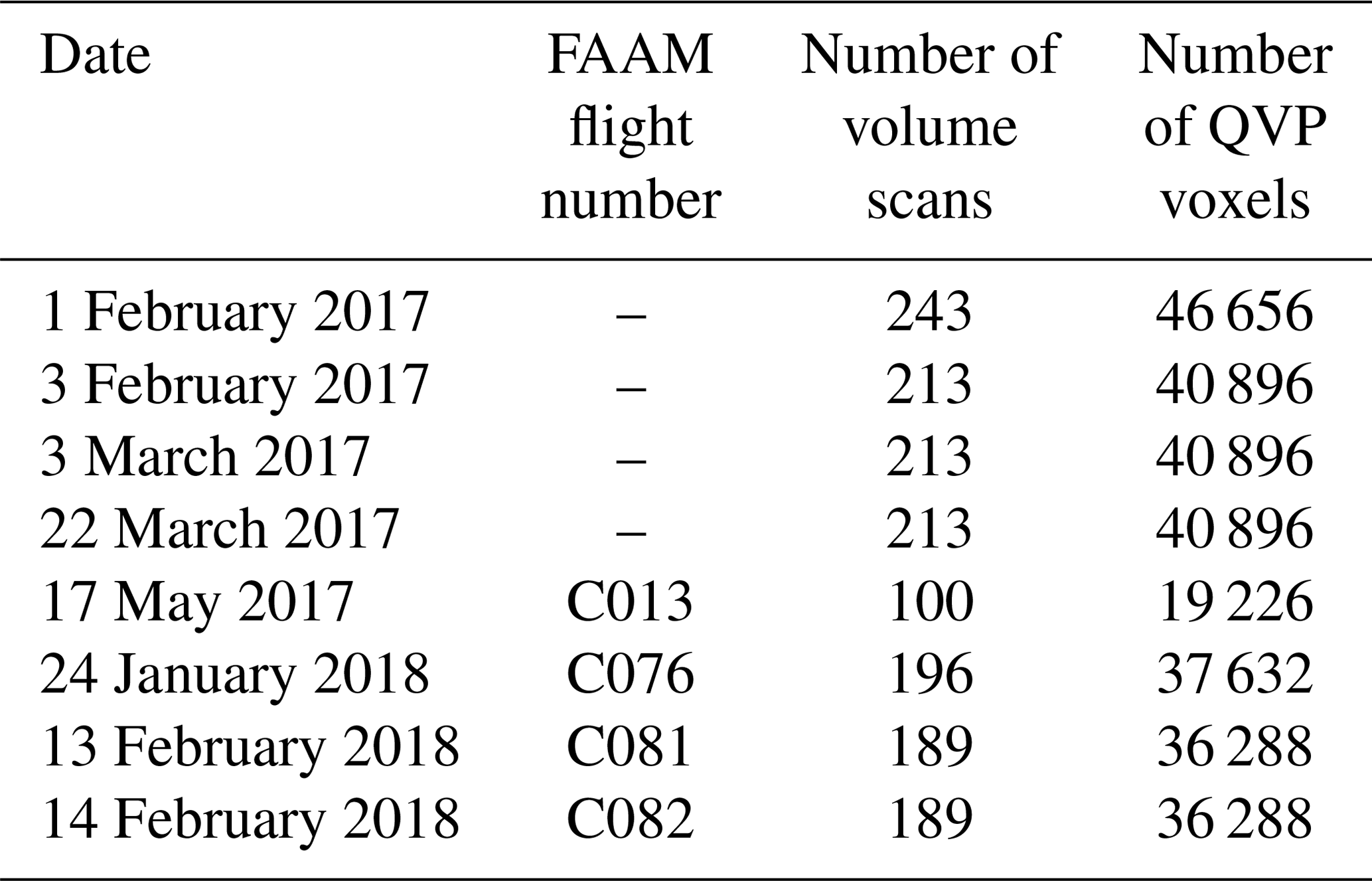
The polarimetric data employed to demonstrate the method developed in this study were collected by the NXPol radar whilst it was located at the Chilbolton Atmospheric Observatory (CAO), part of the UK's National Centre for Atmospheric Science's Atmospheric Measurement and Observation Facility (AMOF), in southern England (51.145∘ N, 1.438∘ W) from November 2016 to May 2018 (Fig. 1). The NXPol is a mobile Meteor 50DX (Leonardo Germany GmbH) X-band, dual-polarization, Doppler weather radar with a 2.4 m diameter antenna. The radar is a magnetron-based system and operates at a nominal frequency of 9.375 GHz (λ∼3.2 cm). The detailed characteristics of the NXPol radar can be found in Neely et al. (2018). From the observations made in 2017–2018 we selected eight dates with the longest precipitation events occurring within a 30 km range of the radar presented on Fig. 1. The exact dates and the total number of volume scans per date can be found in Table 1. Radar data selected for this study can be found in the list of mobile X-band radar observations on the Centre for Environmental Data Analysis (CEDA) archive (Bennett, 2020).
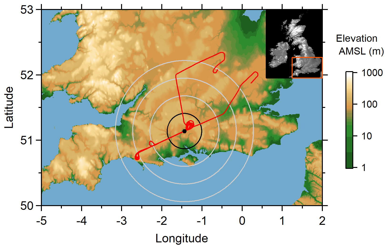
Figure 1NXPol radar location at the Chilbolton Atmospheric Observatory. Circles with their centre on the radar position represent a 30, 60, 90 and 120 km range. Credit: USGS (2006).
3.2 Polarimetric variables and temperature data
Here, we chose to use the polarimetric variables ZH [dBZ], ZDR [dB], ρHV [–], and KDP [∘ km−1] as well as temperature T [∘C] to demonstrate the described clustering technique. The four polarimetric variables were selected as a subset of all the possible variables as they provide complementary information about the observed hydrometeor properties. Here, KDP is calculated as the linear gradient of differential phase shift, where the phase shift has been filtered to remove non-meteorological targets (ρHV>0.85) and progressively smoothed using decreasing length averaging windows, and ZH and ZDR are corrected for attenuation using the standard ZPHI method (Testud et al., 2000), where α=0.27, b=0.78 and specific differential attenuation is 0.14 times the specific horizontal attenuation. Temperature was added to the set of input variables following the reasoning of similar studies in which either the height relative to the 0 ∘C isotherm (Grazioli et al., 2015) or the index representing the ice- or liquid-phase of observed precipitation (Besic et al., 2016) was included. The full input vector used in this study can be represented as follows:
Note that this does not preclude the use of differing sets of variables in future studies. The input data used here were preprocessed before being utilized in the clustering algorithm: all range bins that were located at distances of less than 400 m from the radar were removed from all input variables' data to reduce the influence of side lobe noise.
The temperature data were taken from the Met Office Unified Model (UM) and interpolated onto the polar grid of the radar's observations. The original data can be found on the CEDA archive (Met Office, 2016). Past assessments of the accuracy of these temperature values suggest that the gridded temperatures are within 1 ∘C of coincident profiles measured by radiosondes except in the case of strong inversions or frontal boundaries. An example of observations from 1 d (17 May 2017) represented in the height vs. time format of the QVPs of four polarimetric variables with the temperature presented as isotherms is found in Fig. 2. Similarly, other dates from our list of cases (Table 1) are in Fig. B1.
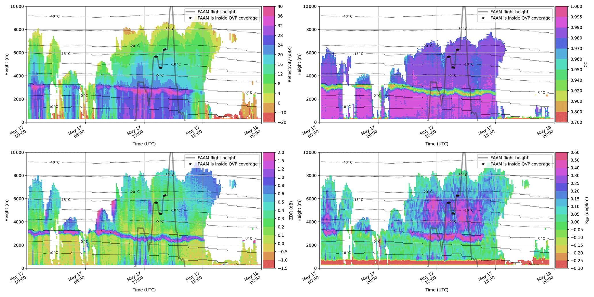
Figure 2The height vs. time QVPs of ZH [dBZ], ZDR [dB], ρHV [–] and KDP [∘ km−1] retrieved from the NXPol radar observations at Chilbolton on 17 May 2017. Overlaid by temperature isotherms T [∘C].
3.3 QVPs and thresholding
QVPs of the input variables are obtained as the azimuthal average of the data from a standard plan position indicator (PPI) scan at a 20∘ antenna elevation angle (Ryzhkov et al., 2016). The 20∘ PPI is the highest of 10 PPIs of the volume scanning strategy used by NXPol which starts the scanning from a 0.5∘ elevation angle. The use of the 20∘ PPI minimizes the effects of radar beam broadening and horizontal inhomogeneity. The beam-broadening effect becomes dominant at higher altitudes when observed by a low-elevation scan as was shown in Ryzhkov et al. (2016). The radar beam of 1∘ opening at 20∘ elevation is about 100 m at 2 km height, 240 m at 5 km height, and reaches almost 480 m at 10 km height. The resulting profiles have 197 voxels in each QVP at the altitudes between 0 and 10 km above mean sea level (a.m.s.l.) and covering about a 30 km range from the radar. It was also shown in Ryzhkov et al. (2016) that the decrease in ZDR from the oblate spheroidal hydrometeors at a 20∘ elevation is within the common measurement error of ZDR (0.1–0.2 dB).
An advantage of QVPs is that they reduce statistical errors within the input dataset, while the height vs. time format of QVPs naturally represents the temporal dynamics of microphysical processes observed in the radar data. To ensure the observations are representative of large-scale meteorological features that may be averaged together, the QVP voxels are used in the analysis only if more than 270 of the 360 azimuthal bins at the range in the PPI scan contain valid data.
3.4 In situ observations
For the labelling of the clusters, in situ observations can be used to assess any of the clusters within the hierarchical structure produced by the clustering algorithm. This allows for flexibility in the granularity used to examine the observations. In this study, the in situ FAAM BAe 146 observations are used to demonstrate the labelling and assessment of the final set of clusters. The FAAM BAe 146 is a publicly funded research facility that, as part of the National Centre for Atmospheric Science (NCAS), supports atmospheric research in the UK by providing a large instrumented Atmospheric Research Aircraft (ARA) and the associated services. The ARA is a modified British Aerospace 146-301 aircraft. Further details of the FAAM BAe 146 aircraft instrument systems are available at https://www.faam.ac.uk/the-aircraft/instrumentation/ (last access: 25 January 2021). In situ data for this study come from FAAM BAe 146 flights C013, C076, C081 and C082 (FAAM, 2017, 2018a, b, c), and observational data are available on the CEDA archive. The dates of the flights and their corresponding flight numbers can be found in Table 1.
For the cases examined, FAAM BAe 146 was equipped with two cloud imaging probes (CIP), which are manufactured by Droplet Measurement Technologies and described in Baumgardner et al. (2001). The CIPs are mounted underneath the aircraft wings and provide 2-bit grayscale images of cloud particles as they pass through the instrument sample volumes. Each CIP houses a 64-element photodiode detector, with one CIP having an effective pixel size of 15 µm (referred to as CIP15) and the other having an effective pixel size of 100 µm (referred to as CIP100). Therefore, the CIPs provide images of particles in size ranges from 7.5 to 952.5 µm for CIP15 and from 50 to 6350 µm for CIP100. All probes have “Korolev” anti-shatter tips – the width of which is 70 mm for the CIP100 and 40 mm for the CIP15.
Particle size distributions are calculated based on CIP data where particle size is defined as being the maximum recorded length in either the axis of the detector array (X) or along the direction of motion (Y). All particles with inter-arrival times s are rejected as indicative of shattering, as in Field et al. (2006). The centre-in approach (Heymsfield and Parrish, 1978) for the estimation of particle concentrations from the sample volume is used to calculate the size of partially imaged particles. It should be noted that despite using the centre-in method with the CIP data, which increases the effective sample volume for larger particles at the expense of uncertainty in particle size, the ability to measure particles with a size >6 mm is negligible with this configuration. An indication of the potential presence of such large particles can be obtained through a visual inspection of the particle images, but no conclusions can be drawn. Also, there are significant uncertainties associated with the derived properties from the CIPs, which are of the order of 20 % for number-based properties (Baumgardner et al., 2017). In our analysis, we are not concerned with absolute concentrations from the CIPs; instead, we are using the CIP data in a qualitative manner to provide a general framework for comparison with the HC results obtained from the radar observations.
As we base our clustering on the QVPs of radar observations, which at each range from the radar are averaged over all available azimuths, a direct comparison to aircraft observations taken at an exact position and time stamp would not make a representative comparison. Thus, for the comparison, we have selected the 20 s intervals from the CIP15 and CIP100 data that correspond to the spatial domain and times of the individual 20∘ PPI scans that are used to create the QVPs. Over these 20 s intervals, the mean number concentrations per particle size bin are calculated (Fig. 10). Figure 9 presents examples of particle imagery from the CIPs, which typically represents less than 1 s of the total 20 s of data and shows derived properties of the particles over the entire 20 s sampling period when the airplane observed the atmosphere over the QVP domain.
In order to provide insight into the nature of the particle imagery, we have separated the particle concentrations in Fig. 10 into three categories, two of which are based on an analysis of the particle shapes and another which is for partially imaged particles. “Round” particles are those which have a circularity between 0.9 and 1.2, and particles with a larger circularity are labelled as “Irregular” – this gives a rough separation into particles that are likely to be liquid water vs. ice (Crosier et al., 2011). “Edge” particles are those which are only partially imaged, as indicated by pixels at the extreme edge of the array being triggered. For the particles that are considered round, the particle size and subsequent concentration is corrected for out-of-focus effects (Korolev, 2007). This out-of-focus correction is not applied to the “irregular” or “edge” images, as there is no evidence to show that this is an appropriate correction to make. For two key reasons, no attempts have been made to classify particle images. (1) The larger particles, which have the greatest influence on the polarimetric properties, are poorly sampled by the CIPs. (2) A recent study by O'Shea et al. (2020) suggests that existing procedures to classify particle images using the CIP can lead to inaccurate results due to the effects of diffraction when particles are imaged more than a few millimetres off the focal plane, which is the most common scenario. A thorough assessment of the accuracy of these image classification algorithms, with respect to particle size and probe configuration, is much needed.
Here, the clustering steps are described in general. A corresponding overview of the approach is provided in Fig. 3. The proposed approach uses QVP voxels and temperature data that have been interpolated to the same volume. These data form the points of a five-dimensional space (d=5). The PCA (Sect. 2.2) reduces the number of dimensions to q. The q-dimensional data are partitioned into K clusters, where K iteratively increases () until the optimal number of clusters is reached, according to the WG index Eq. (1) in Sect. 2.4. With each of the clusters achieved in this level (“outer loop” in Fig. 3), the process is recursively repeated starting with the PCA calculation and continuing until the optimal partitioning of the sub-clusters is reached (“inner loop” in Fig. 3). The total partitioning is confirmed with the BIC index Eq. (2) in Sect. 2.4. When the BIC's local maximum is reached, the partitioning is considered to be optimal. A detailed description of each of these steps can be found in the following subsections, and the code can be made available upon request.
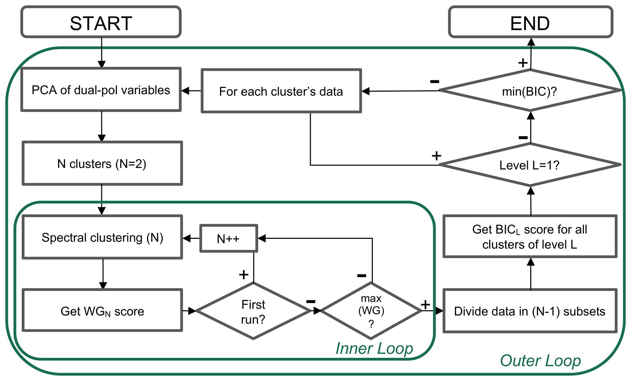
4.1 Start of hierarchical clustering
The hierarchical clustering starts with data standardization and dimensionality reduction of the original five-variable input data X Eq. (3) into a q-dimensional dataset of principal components (Sect. 2.2). The non-parametric transformation based on the quantile function maps the data to a uniform distribution. This standardization helps to deal with outliers and satisfy PCA data assumptions.
To start the loop, all N pixels of the input data are used. In later loops, only subsets of the original five-variable data () belonging to active cluster ck are processed in the inner loop (Fig. 3). The first q principal components with the largest variance, which have at least 85 % representativity of the original dataset in total, are selected in this step.
The representativity threshold of 85 % was chosen arbitrarily as it reduces the initial five-variable input space up to three-dimensions (q=3) in most cases, which effectively simplifies the clustering problem and does not influence the overall outcome. The threshold can be reduced to further decrease the dimensionality, but it was found that this negatively influences the clustering accuracy. A higher threshold will retain the high dimensionality of the original dataset but will slow down the clustering process without gaining further information from the dataset.
4.2 Iterative process to find the optimal number of clusters (inner loop)
At the start of the hierarchical clustering, we begin directly with the first call of the inner loop (Fig. 3). The iterative process in the inner loop commences with all N QVP pixels represented by the first q principal components. The spectral clustering processes these input data starting with the number of clusters K=2. The number of clusters increases () with each cycle of spectral clustering within the inner loop, and the WG index Eq. (1) is calculated at the end of each iteration for the achieved clustering CK. At the moment the local maximum is achieved in the WG index values, the clustering in which it was reached () is accepted as the main cluster set of the current level of the hierarchical tree, and these clusters become the set of active clusters (A). Set A will be used in the outer loop of the implemented hierarchical algorithm. The active clusters detected in the first level of the hierarchical structure by spectral clustering for the data on 17 May 2017 are shown in Fig. 4.
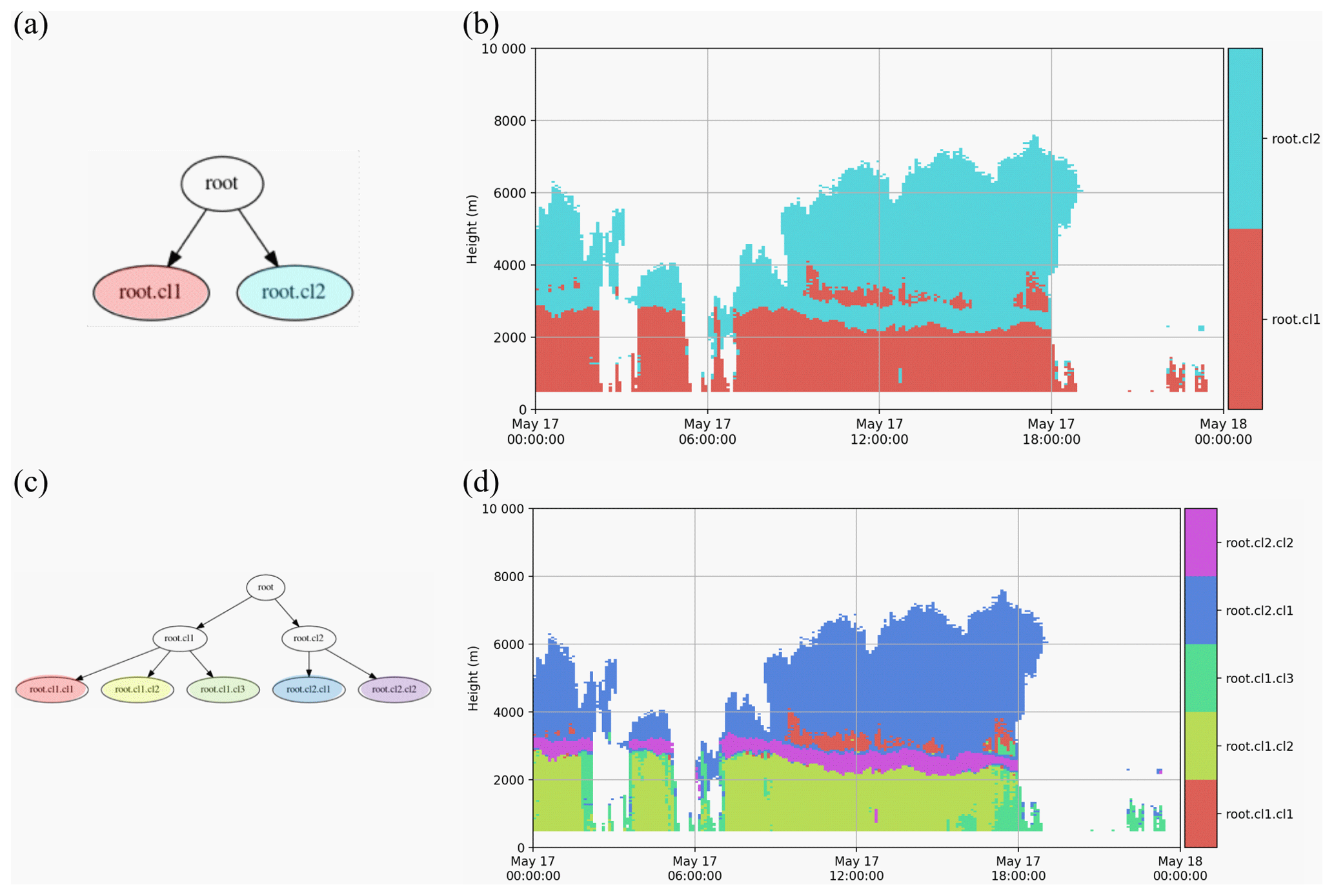
Figure 4The active clusters at the end of the first (a, b) and second (c, d) cycle of the outer loop of the hierarchical clustering algorithm. Panels (a) and (c) are plotted in the hierarchical (tree) structure, and panels (b) and (d) are plotted in height vs. time format of the observations on 17 May 2017.
4.3 Optimal number of clusters for the total dataset (outer loop)
In the outer loop of the hierarchical algorithm, the BIC index Eq. (2) is calculated for the active clusters produced by the inner loop (Fig. 3). If the BIC index is calculated for the first time (i.e. the start of the algorithm run, j=1) or the BIC index values do not show any local maximum, the algorithm continues by calling the inner loop for each individual cluster from the set of active clusters (Aj) formed by the calls of the inner loop described above.
For the first level of hierarchical clustering, all are immediately accepted as active . In the outer loop, after calculating the BIC, the original five-dimensional data belonging to each cluster are sent to the inner loop and clustering () achieved by the inner loop is used to replace the cluster in the set of active clusters A1. If the BIC index calculated on this “suggested set” shows that the clusters introduced to the A1 increase the value of BIC, the suggested replacement is accepted and the set of active clusters is updated as . The outer loop then continues with the next cluster from the original set A1. When the BIC value does not increase with the “suggested set”, the set of active clusters does not change, and the algorithm continues with the next cluster from the set A1.
4.4 Next recursion or finalization of results
The final set of active clusters is reached when the value of the BIC index does not increase with any further suggested split in the current active set of clusters. At this level of “detailization”, the optimal clustering for the provided input data has been reached. For the QVP dataset described in Sect. 3, a final set of 13 active clusters is reached (see Figs. 5 and 6). The relations between these final clusters (f_cl1,…, f_cl13) and the three parent clusters from the first inner loop run (Fig. 4a) are shown in Fig. 5.
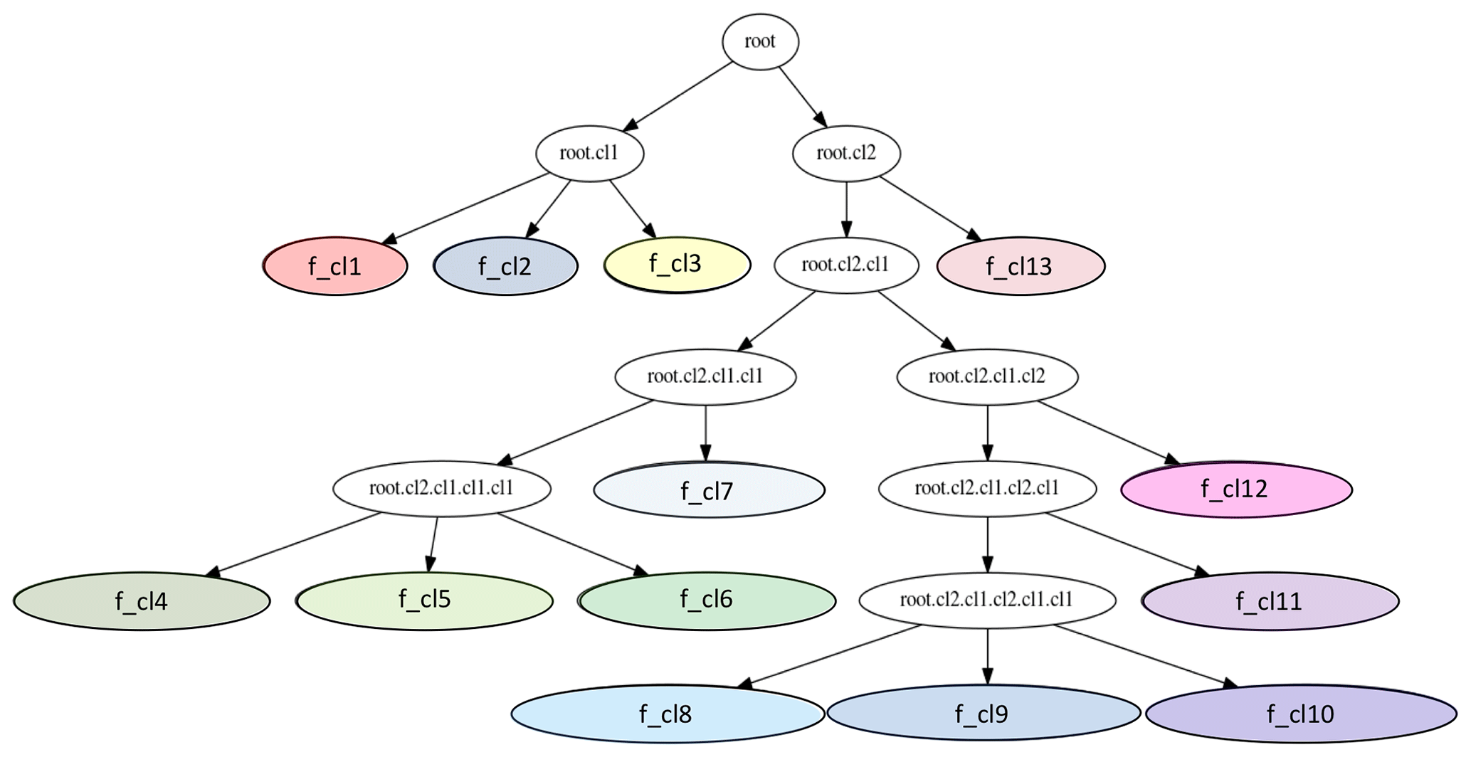
Figure 5Final hierarchical structure of the optimal clustering found for the QVP input data described in Table 1. The final set of optimal clusters consists of coloured clusters f_cl1, f_cl2,…, f_cl13.

Figure 6The height vs. time format of the final optimal set of active clusters found by the top-down hierarchical clustering for the QVP input data described in Table 1. (The hierarchical structure behind the optimal clustering is found in Fig. 4.) Example of clusters in the height vs. time format of the 17 May 2017 QVPs presented in Fig. 2.
Once the optimal number of clusters is determined and the hierarchical clustering structure is built, the clusters can be characterized by their centroids and labelled with appropriate hydrometeor classes using the available verification data. The clusters for which direct verification data are not available may still be labelled with an appropriate hydrometeor class based on the scattering characteristics described by the original polarimetric radar variables and considering their position in the hierarchical tree and the height vs. time QVP representation. As QVP polarimetric characteristics differ from polarimetric characteristics of hydrometeors observed by PPI and RHI scans, care must be taken when comparing these results to the literature. Labelling the obtained clusters can be performed for the different levels of granularity depending on the user's needs and interests. Note the purpose of the labelling shown here is to demonstrate the ability and validity of the technique rather than performing a rigorous study of the underlying microphysics observed. The latter will be reserved for follow-up studies utilizing this technique in a focused manner.
5.1 Level-by-level cluster check
From the visual verification of the first-level parent clusters in Fig. 4a and b, we can deduce that there are two child clusters representing the upper or elevated (ice-dominated root.cl2) and the lower (water-dominated root.cl1) parts. The second-level clusters from the second loop (Fig. 4c and d) show a well-identified “bright band” (root.cl2.cl2), belonging to the melting layer (ML), and a main solid-phase cluster (root.cl2.cl1), both belonging to the cluster representing the ice-phase-dominated part (root.cl2) of the QVPs (Fig. 4b). The three child clusters of the parent root.cl1 cluster (Fig. 4c and d) are the two rain-type clusters (root.cl1.cl2 and root.cl1.cl3) below the “bright band” and cluster root.cl1.cl1 with most points located above the “bright band”. In further loops, the main ice-phase cluster (root.cl2.cl1) is split into nine child clusters (Fig. 5), and examples of their positioning in the height vs. time format of QVPs can be observed in Fig. 6 or Fig. B1.
5.2 Characteristics of the clusters
The 13 final clusters can be characterized by their centroids (Fig. 7) or their relevant statistics (Fig. 8, Table A1). The centroid characteristics in Fig. 7 are plotted as spider plots where each of the five variables is represented by an azimuthal axis. The filled pentagons in each sub-plot represent the cluster's centroid in the five-variable space based on all the data available in this study. Each vertex of the pentagon shows the centroid's value in one of the five variables. The non-solid lines in the sub-plots of Fig. 7 represent the centroids of the same cluster but based solely on the data from one of the eight cases (Table 1).
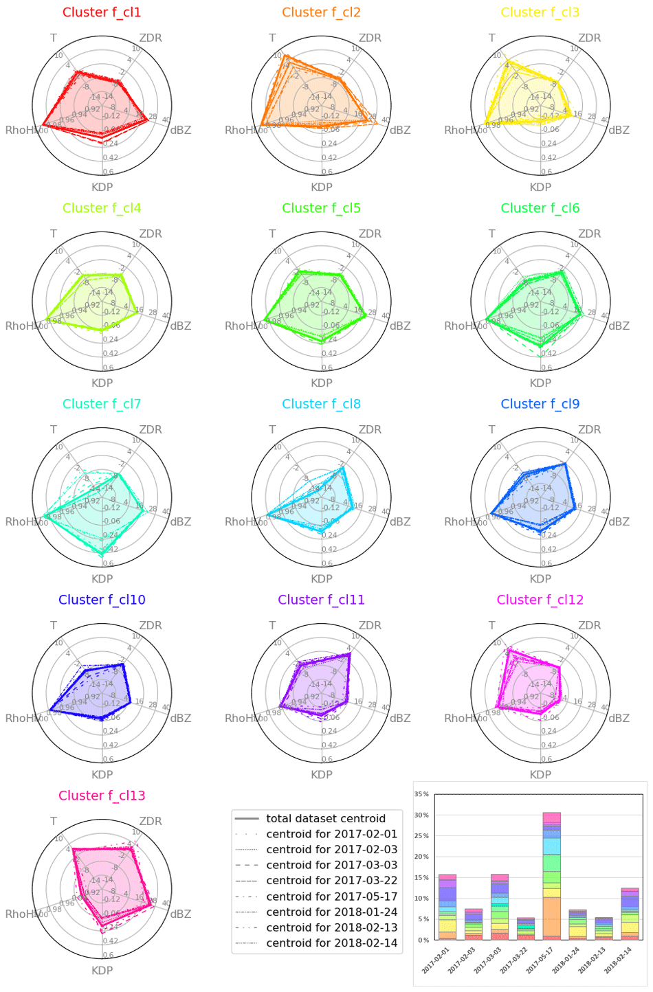
Figure 7Characteristics of the optimal clustering centroids in four polarimetric variables and temperature. The scales of the variables are as follows: from −20 to 40 dBZ for ZH, from −1.5 to 2.0 dB for ZDR, from 0.9 to 1.0 for ρHV, from −0.3 to 0.6∘ km−1 for KDP and from −20 to 10 ∘C for temperature (T).
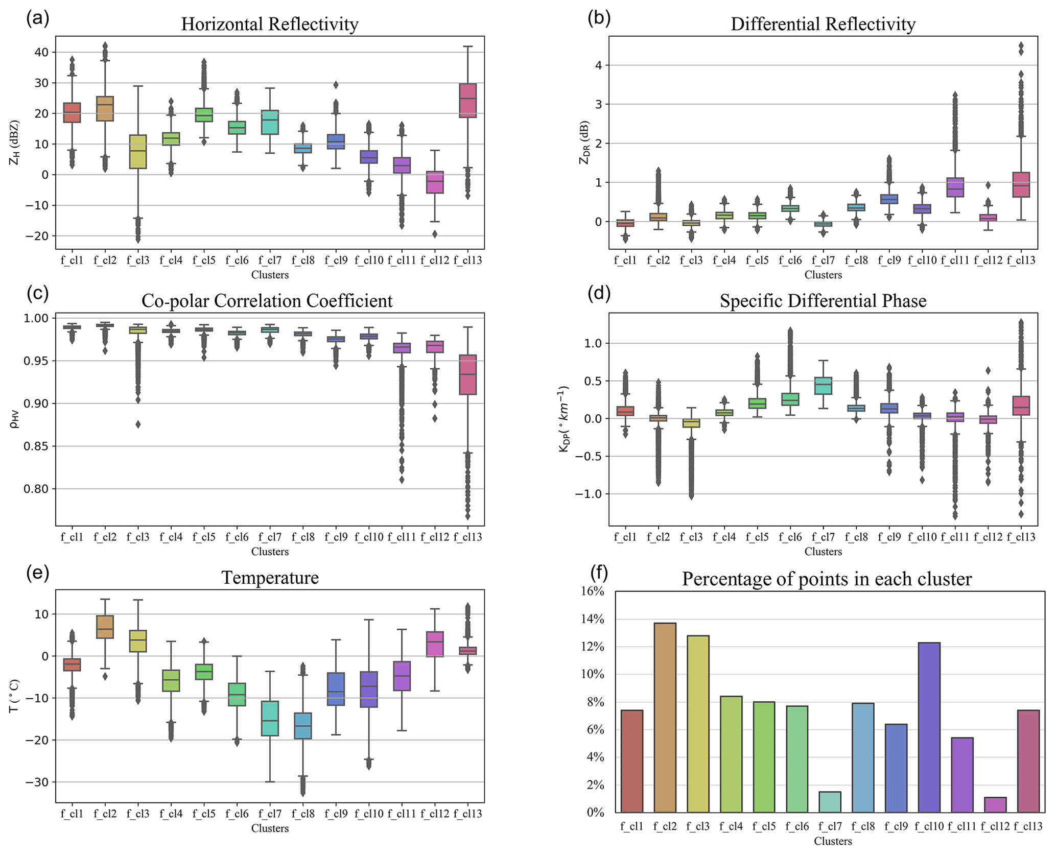
Figure 8Characteristics of the optimal clustering centroids in four polarimetric variables (a – ZH, b – ZDR, c – ρHV and d – KDP) and temperature (e). The percentage of points in each cluster is shown in panel (f).
Figure 7 confirms a distinction made at the first and the second cycles of the outer loop (Fig. 4) between three types of clusters: liquid-phase clusters (f_cl1, f_cl2 and f_cl3), with lower KDP and warmer T values; ice-phase clusters (f_cl4, f_cl5, f_cl6, f_cl7, f_cl8, f_cl9, f_cl10, f_cl11, and f_cl12), all with more pronounced ρHV values; and a very different looking f_cl13, with warmer T and rather low ρHV values.
The largest differences between the centroids selected from the total dataset and the centroids corresponding to the eight considered cases occur in the temperature (T) values, especially for the clusters f_cl2, f_cl3, f_cl7, f_8, f_cl10 and f_cl12. These variations can be explained by the origin of the temperature data, which are estimates from the NWP model and do not always correctly represent the real situation.
The next variable with a rather large variation in several clusters is KDP. In part, this variation may be due to the fact that this variable has an extremely skewed distribution. Clusters f_cl1, f_cl7, f_cl11, f_cl12 and f_cl13 have the highest variation in KDP values between the centroids calculated for different cases (Fig. 7). As KDP can be influenced by the amount of ice or water particles in the atmosphere, it might be that the clusters have variations in the number of particles. This hypothesis can only be verified with FAAM BAe 146 observations of the same cluster on different dates. Unfortunately, such verification is not possible for all clusters, and more in situ observations are required.
From the variations of centroid values in the five input variables in Fig. 7, we can also see that the main liquid-phase cluster (f_cl2) has rather different characteristics in different cases. Case to case it shows large variations in ZH, KDP, ρHV, T and the highest mean temperature value (6.8 ∘C) among all other clusters. As observed in the histogram of percentages of the cluster points in Fig. 8f, f_cl2 is rather big (13.7 % of the total number of points) but does not have the highest percentages of points in all eight analysed cases, only in the 17 May 2017 case (9.3 % compared with ≤1.5 % in other cases) (Fig. 7, histogram in the lower right corner.). Combining all of these aspects, we deduce that f_cl2 includes rain of varying intensities and different drop sizes.
The other rain cluster f_cl3 has less variability in centroid values and has ∼20 dBZ smaller ZH values than f_cl2, which is probably due to the smaller drop sizes in this cluster. f_cl3 has the smallest mean ZH (7.18 dBZ) and mean KDP values (−0.097∘ km−1) of all “water” clusters (f_cl1, f_cl2 and f_cl3). This cluster is often observed at the beginning and at the end of the storm in the height vs. time format representation of the optimal clusters (Fig. B1) and is labelled as “light rain”.
Almost all centroids in Fig. 7 have no or very limited variation in the ρHV or ZDR values except for f_cl13. This cluster has no variation in temperature (T), with all centroids at 0 ∘C. As such, f_cl13 corresponds to the area in the data referred to as a “bright band”. According to the box and whiskers plots in Fig. 8, cluster f_cl13 has the highest mean ZH (24 dBZ) and mean ZDR (0.99 dB) as well as the lowest mean ρHV (0.93) compared with the other optimal clusters, and it is mostly located near 0 ∘C. These characteristics immediately indicate that f_cl13 can be labelled as belonging to the “bright band” cluster with mixed-phase (MP) particles.
The MP cluster (f_cl13 in Fig. 6) is observed to have some sagging areas: between 10:00 UTC and 12:20 UTC, around 16:00 UTC and near 18:00 UTC. Note that f_cl1 is observed above the MP cluster f_cl13 exactly at these time intervals (Fig. 6). This sagging “bright band” signature is often observed where aggregation and riming processes are occurring directly above the melting layer (Kumjian et al., 2016; Ryzhkov and Zrnic, 2019). This suggests that f_cl1 can be associated with the processes of aggregation or riming and labelled accordingly.
Looking at the percentage of points belonging to each cluster in the optimal clustering set (Fig. 8f), we see that clusters f_cl7 and f_cl12 have less than 2 % of points and most probably represent some sporadic and/or special conditions. These clusters have also been separated early from the other “low ice” (f_cl4, f_cl5, f_cl6) and “elevated ice” (f_cl8, f_cl9, f_cl10, f_cl11) clusters and are located near the top of the hierarchical tree (Fig. 5). Both clusters f_cl7 and f_cl12 have smaller absolute mean ZDR values (−0.062 and 0.097 dB respectively) than the other “ice” clusters (Fig. 8b). f_cl7 is also characterized by the highest mean KDP value (0.44∘ km−1) among all of the clusters (Fig. 8d). The combination of rather high ZH (17 dBZ) and high KDP at temperatures around −15 ∘C indicates a cluster with high particle number concentration of small ice crystals mixed with a small amount of bigger aggregates. This cluster is potentially a manifestation of the rapid growth of ice via vapour deposition and the onset of aggregation in the dendritic growth layer (DGL) discussed in detail in Griffin et al. (2018). These characteristics were also recognized as a signature of dendritic crystals in Bechini et al. (2013). f_cl12 has the lowest mean ZH value (−3 dBZ) of all optimal clusters. Combining the low mean ZH with low mean ZDR (0.097 dB) and a temperature of about 3 ∘C, we can assume that f_cl12 can be labelled as small droplets (i.e. drizzle).
f_cl11 belongs to the “elevated ice” clusters and in most cases (see Appendix B, Fig. B1) appears as a column in the height vs. time representation (around 07:00 UTC in Fig. 6 or in panels (a) 07:00–08:00 UTC, (c) 05:00 and 07:30 UTC, (g) 12:00 UTC and (h) 12:00–12:30 UTC in Fig. B1) filling all of the altitudes from the top of the cloud to the ML. This cluster has a low mean ZH value (3 dBZ), one of the highest mean ZDR values (0.92 dB) and a close to zero mean KDP value (−0.009∘ km−1). f_cl11 can be labelled as the pristine ice crystals class, as they typically have high aspect ratios (≫1) and tend to fall preferentially with their major axis aligned horizontally (Keat and Westbrook, 2017).
Clusters f_cl8, f_cl9 and f_cl10 belong to the “elevated ice” branch of the hierarchical tree (Fig. 5). Among these clusters, f_cl9 has the most different characteristics compared to the f_cl8 and f_cl10 clusters. f_cl9 has higher mean ZH (11 dBZ) and ZDR (0.59 dB) in combination with a lower ρHV (0.97).
f_cl8 and f_cl10 have rather similar characteristics to each other (Fig. 7, Table A1). The small difference between these two clusters is in a higher mean ZH (8.6 dBZ) and KDP (0.14∘ km−1) for f_cl8 compared with 5.8 dBZ and 0.028∘ km−1 for f_cl10. Both clusters are the main “elevated ice” clusters. f_cl10 has a warmer mean temperature (−8.2 ∘C compared with −16.7 ∘C for f_cl8), and most of the time it is located near f_cl8 at the beginning or at the end of the observed event (Fig. B1).
The main “low ice” clusters are f_cl4, f_cl5 and f_cl6. Clusters f_cl5 and f_cl6 are often observed together with f_cl6 located above f_cl5. f_cl4 has several appearances in the height vs. time formats of events (see Appendix B, Fig. B1, e.g. 09:00 UTC in panel a, 11:00 UTC in panel b, 09:00 and 17:00-18:00 UTC in panel e), mostly above f_cl1, reaching higher altitudes in the data.
Measurement errors may influence the clustering results. As was shown by Bringi et al. (1990), noise in the observations has a strong impact on k-mean HCA (hierarchical clustering algorithm) results. Unfortunately, it is impossible to run the same type of analysis conducted by Bringi et al. (1990) for an unsupervised hierarchical clustering algorithm, as the added noise might deliver a modified hierarchical structure with another optimal number of clusters, and direct comparison to the original set of final clusters would be impossible. Here, this issue of noise is partially addressed through our use of QVPs. In particular, azimuthal averaging of a QVP reduces the noisiness of the differential phase within the melting layer (Trömel et al., 2013, 2014) and was recommended in Kumjian et al. (2013) to quantify rather small enhancements of ZDR and KDP.
The mean negative values of ZDR and KDP in some clusters (f_cl1, f_cl3 and f_cl7) might point at potential biases due to the miscalibration of ZDR, differential attenuation or backscatter differential phase in the melting layer. Biases in the data such as miscalibration will not impact the clustering process but will impact the labelling, as it is based on cluster characteristics. A miscalibration of ZDR can also be excluded, as we routinely perform calibration of this variable. ZH and ZDR are corrected for the attenuation in the data preprocessing. Biases caused by backscatter differential phase in the melting layer (Trömel et al., 2014) have not been removed and are evident in the cluster characteristics. The influence of the backscatter differential phase needs further investigation. As discussed, not all clusters can be labelled with absolute confidence solely based on the cluster's characteristics, and in situ observations can help to verify these initial suppositions.
5.3 Clusters vs. in situ observations
5.3.1 In situ data
For the verification of the preliminary labelling made in Sect. 5.2, data from the CIP15 and CIP100 on board the FAAM BAe 146 are utilized. FAAM BAe 146 aircraft flights were performed on 4 out of 8 d (Table 1) of radar observations: 17 May 2017, 24 January 2018, 13 February 2018 and 14 February 2018. The flight altitudes and the time stamps when the aircraft was inside the QVP domain can be observed in the height vs. time representations of the optimal clusters in Fig. B1.
Out of the four available flights, there are 23 periods of 20 s intervals which result in a total of 460 s of flight time when the aircraft was inside the QVP domain and a cluster can be assigned to the corresponding height. Of these 23 periods there are observations corresponding to nine unique clusters (f_cl1, f_cl2, f_cl3, f_cl4, f_cl5, f_cl6, f_cl8, f_cl10, f_cl12). This samples 70 % of the final clusters. From these time series, we present examples of CIP15 and CIP100 images for each cluster (Fig. 9) and mean particle size distributions of the data observed during the 20 s interval (Fig. 10).
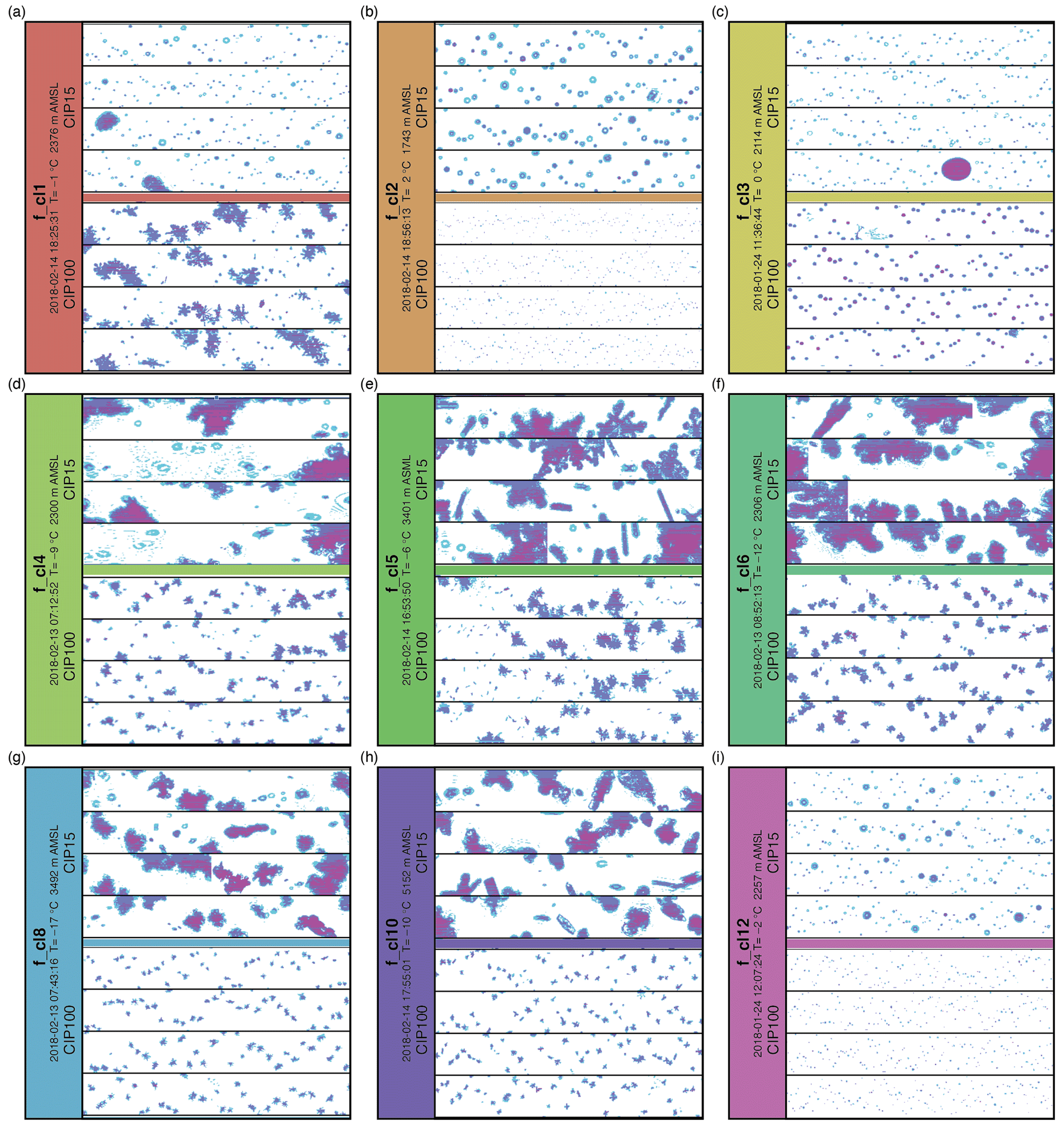
Figure 9Examples of the images taken from the cloud image probe CIP-15 (15 µm, upper) and CIP-100 (100 µm, lower) within a 30 km range of the radar position: (a) for f_cl1 – at 18:25:31 UTC on 14 February 2018; (b) for f_cl2 – at 18:56:13 UTC on 14 February 2018; (c) f_cl3 – at 11:36:44 UTC on 24 January 2018; (d) f_cl4 – at 18:17:53 UTC on 14 February 2018; (e) f_cl5 – at 16:53:50 UTC on 14 February 2018; (f) f_cl6 – at 08:52:13 UTC on 13 February 2018; (g) f_cl8 – at 07:43:16 UTC on 13 February 2018; (h) f_cl10 – at 17:55:01 UTC on 14 February 2018; (i) f_cl12 – at 12:07:24 UTC on 24 January 2018. The image widths are 960 and 6400 µm respectively. The temperature values are derived from the model data, and the heights are derived from the location of the clusters in the QVPs.
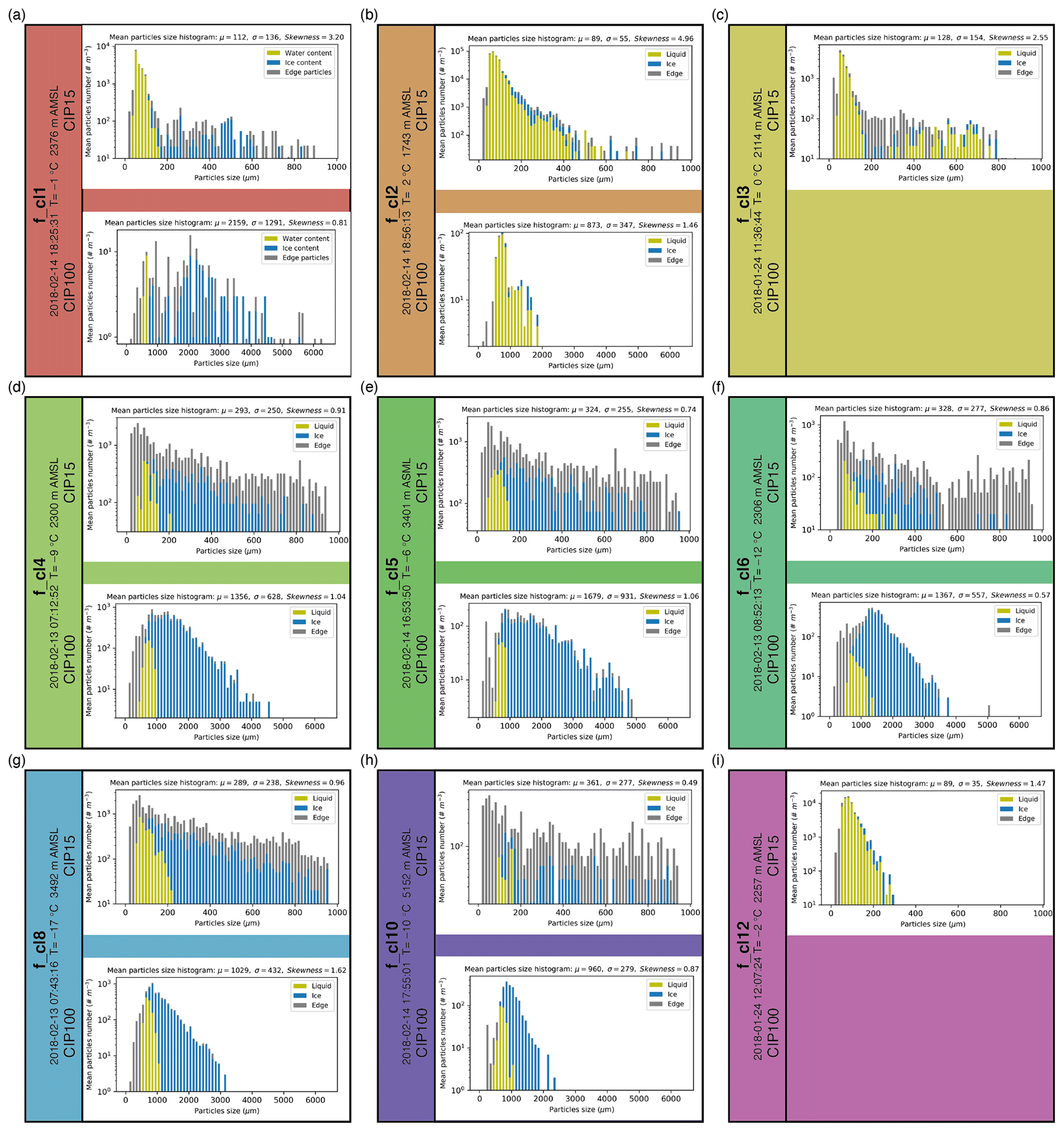
Figure 10Corresponding to Fig. 9, particle size distributions from the cloud image probe CIP-15 (15 µm, upper) and CIP-100 (100 µm, lower) within a 30 km range of the radar position: (a) for f_cl1 – at 18:25:31 UTC on 14 February 2018; (b) for f_cl2 – at 18:56:13 UTC on 14 February 2018; (c) for f_cl3 – at 11:36:44 UTC on 24 January 2018; (d) for f_cl4 – at 18:17:53 UTC on 14 February 2018; (e) for f_cl5 – at 16:53:50 UTC on 14 February 2018; (f) for f_cl6 – at 08:52:13 UTC on 13 February 2018; (g) for f_cl8 – at 07:43:16 UTC on 13 February 2018; (h) for f_cl10 – at 17:55:01 UTC on 14 February 2018; (i) for f_cl12 – at 12:07:24 UTC on 24 January 2018. The image widths are 960 and 6400 µm respectively. The temperature values are derived from the model data, and the heights are derived from the location of the clusters in the QVPs.
5.3.2 Liquid-phase clusters
The liquid-phase clusters f_cl1, f_cl2 and f_cl3 correspond to in situ data that contain relatively high concentrations (>1000 m−3) of small particles (mostly <200 µm in size) which appear round (Figs. 9a–c, 10a–c). This strongly reinforces the idea of large amounts of liquid water being present in the cloud, which supports the labelling of f_cl1–f_cl3 as being influenced by liquid water hydrometeors. When looking at CIP100 in situ observations in detail, and to some extent CIP15 observations at sizes >200 µm, we can see some significant difference between clusters f_cl1–f_cl3, which we will now discuss.
f_cl1, observed above the “bright band”, was previously assigned to be the result of aggregation and riming. In this region, the CIP100 (Fig. 9, lower part of panel a) shows particle imagery and particle size distributions segregated by shape that show the presence of large ice particles (Fig. 10a), again confirming the previous cluster labelling. The CIP100 data show the presence of irregularly shaped particles, ranging in size from ∼1 to 4 mm, with concentrations in each bin of the order of 1 m−3. This suggests that a mode of snow particles is present at the same time as the previously mentioned liquid droplet mode. Many small water droplets in the CIP15 observations (Figs. 9a and 10a, CIP15) could indicate either the presence of warm cloud processes or small ice crystals melting first around the ML. The second interpretation is supported by the imagery from the CIP100 which suggests melting has not started to occur on the larger particles. In this case, the larger aggregate snowflakes fall to lower altitudes before they start to melt and form the clear “bright band” in the QVPs.
f_cl2 was characterized by the strong variation in ZH, KDP, ρHV and T of the cluster's centroids in different cases. Both CIP15 and CIP100 have small round-shaped particles in the corresponding images (Fig. 9b). The mean concentrations per particle size distributions (Fig. 10b) show the prevalence of particles recognized by shape as water droplets. The droplets of <2 mm size have the occurrences of the order of 10 to 90 000 m−3, with higher orders corresponding to particle sizes <200 µm. Summing up previous analysis and in situ observations, we can assign f_cl2 to a “liquid” cluster, which includes rain of varying intensities and different drop sizes.
f_cl3 also has predominantly small round-shaped particles (mean size μ=128 µm) in the CIP15 panels (Figs. 9 and 10, upper part of panel c). The CIP100 data (Fig. 9, lower part of panel c) were not processed due to technical issues with the probe, so water or ice concentrations based on this data are unfortunately not available. The high concentrations (1000–5000 m−3) of small size (<200 µm) particles are assigned to water (Fig. 10c). Concentrations of the larger particles (>200 and <800 µm) are very low (<100 m−3). Considering these observations, the cluster's characteristics, and the fact that the cluster appears mostly at the beginning or at the end of the events (Fig. B1), we can assume that the cluster either represents very light rain or drizzle or indicates a partially filled QVP domain in the original data.
5.3.3 Solid-phase clusters
The CIP15 images for f_cl4 show a mix of larger irregularly shaped particles (aggregates of snowflakes) and relatively few tiny ice crystals (Fig. 9d) with very small irregular shapes. The mix of small (<1 mm) particles recognized as water and ice has low total concentrations (500–800 m−3; Fig. 10d). Particles of larger sizes (>1 and <3.0 mm) have concentrations from 100 to 800 m−3 (Fig. 10, lower part of panel d) and were recognized as ice due to their irregular shapes. The small number of “round” particles recognized as liquid are likely an artefact of the data processing due to out-of-focus imaging of the numerous ice particles which are present – such artefacts appear when particles are observed at the edges of the depth of field (O'Shea et al., 2019). Accordingly, this cluster can be assigned to the mix of pristine ice and some formed aggregates, all with low concentrations.
f_cl5 and f_cl6 show very similar images in CIP15, but the CIP100 images illustrate the difference between these two clusters (Fig. 9e, f). The shape analysis of CIP100 suggests that both clusters include a low concentration (40–50 m−3) of small round-shaped particles (<1 mm size; the lower part of panels e and f, Fig. 10). Similar to f_cl4, the number of liquid particles are likely an artefact of the data processing (O'Shea et al., 2019). The main difference between these clusters is shown in the part of the data recognized as ice. The mean size of the particles of f_cl5 is about 1.7 mm and has occurrences of the order of 100 m−3 (Fig. 10e). The mean size of particles in f_cl6 is a bit smaller (1.4 mm), and particles around that size have a higher occurrence of the order of 400 m−3 (Fig. 10f). This difference between f_cl5 and f_cl6 resembles the aggregation processes when dendritic crystals of higher concentrations formed at higher altitudes (f_cl6) start to clump together during their fall and form aggregates (f_cl5) with a lower concentration of particles.
Clusters f_cl8 and f_cl10, which belong to the “elevated ice” branch of the hierarchical tree (Fig. 5), are also represented by the very similar images of CIP15 and CIP100 observations (Fig. 9g, h) with the difference in the particles' concentration (Fig. 10g, h). f_cl8 has a higher concentration of small size (<1 mm) particles (up to 1000 m−3) recognized as spherical than f_cl10 (up to 300 m−3). The bigger particles captured in CIP100 corresponding to f_cl8 are larger (from 1 mm up to 3 mm) and also have a higher concentration (<500 m−3) compared with particles of f_cl10 that have a maximum size of about 2 mm with concentrations <200 m−3. The example of CIP100 images suggests that these particles are dendritic in nature (Fig. 9h). Again, similar to the artefacts discussed when looking at the CIP observations for f_cl4, f_cl5 and f_cl6, there is likely an erroneous classification of small size particles (O'Shea et al., 2019). Thus, according to in situ data, f_cl8 can be assigned to a mix of pristine ice and bigger aggregates, and f_cl10 can be assigned to a low concentration mix of pristine ice and smaller aggregates.
The last in the list of clusters verifiable with the FAAM BAe 146 data is f_cl12 (Fig. 9i). Figure. 10i shows occurrences of the order of 10 000 m−3 for very small particles up to 150 µm and occurrences of the order of 1000 m−3 for droplet sizes between 150 and 250 µm with almost no occurrence of bigger particles. Unfortunately, concentrations from CIP100 data are not available for this cluster due to technical issues with the CIP100 probe. f_cl12 contains the lowest number of data points in QVP analysis (Fig. 8f), and there are no other in situ observations related to this cluster. Based on available data, we could assume that the cluster has a high concentration of tiny water droplets (potentially drizzle). On the other hand, similar to the data for other classes, the CIP analysis may have misclassified these as liquid due to their small round appearance in the observations when in reality the observations could represent high concentrations of small ice particles. Likewise, the mean temperature of this cluster is close to 0 ∘C, so no definitive label may be given based on the observations. Thus, the physical interpretation of this cluster is ambiguous, although the cluster is separate within the multivariate space.
5.3.4 Assignment conclusions
The rest of the clusters need to be assigned by means of human interpretation according to the cluster characteristics or deduction from the interactions and temporal evolution of already assigned clusters. The summary of the assigned clusters can be found in Table A1 of the Appendix A. Application of in situ observations for the assessment of QVP-based clusters has its limits, as not all optimal clusters were captured by the FAAM BAe 146 flights, and this process requires a comparison of data from essentially one-point measurement to the cluster based on the mean QVP domain values. An appropriate validation process would utilize columnar vertical profiles (CVPs) as described in Murphy et al. (2020) with the thorough co-location of the aircraft observations. Utilizing CVPs within the presented technique is a part of the planned work for the future.
This paper presents a new hydrometeor classification technique from QVPs. Note that both the data-driven approach and the use of QVPs is novel. In this technique, the hydrometeor types are identified from an optimal number of hierarchical clusters, obtained through a recursive process. This recursive process includes an initial dimensionality reduction by principal component analysis followed by spectral clustering. Spectral clustering performed in the PCA space allows us to identify clusters that would have a non-convex form in the original multivariate input space. This property of the algorithm makes it unique and advantageous in comparison to other classification methods, which separate classes by hyperplanes.
The final set of clusters is identified with an optimality check using validity indexes. This represents the first attempt, in top-down hierarchical clustering of weather radar data, to identify the number of clusters based solely on the embedded data characteristics. This data-driven technique produces an optimal number of clusters and keeps the hierarchical structure built in the clustering process. The final set of clusters may be labelled based on their positioning in the hierarchical structure, the characteristics of their centroids and coincident in situ observations. Depending on the user's needs and interests, the labelling can also be performed for different levels of granularity. In the example shown in this study, we utilize observations collected during several FAAM BAe 146 flights to demonstrate the advantages this technique has in the labelling process. In this case, based on the data available, 70 % of the clusters were labelled using the coincident CIP observations. The other 30 % of the clusters, which were not sampled during the FAAM BAe 146 flights of this study, were labelled based on the cluster characteristics, their positioning in the hierarchical structure and considering interactions with clusters in a height vs. time format of original QVP data.
Thus, in this study, we find that a data-driven HC approach is capable of providing an optimal number of classes from the observations. Moreover, the embedded flexibility in the extent of granularity is the main advantage of the technique. Each branch of the hierarchical structure can be cut out at any level, and the parent cluster characteristics can be used for labelling and identifying more general processes in the atmosphere, while the lower level clusters can provide information about more specific properties and features of the observations.
The centroids of the clusters represent characteristics of the points belonging to a cluster in the multivariate input space (in this case, the polarimetric radar variables and temperature). The identification of these centroids allows the clusters to be tracked in time and altitude as the centroids are calculated based on QVPs from single scans. An analysis of the time series of the radar volume scans is possible and would allow the clusters to be tracked in time and three-dimensional space. Although unexplored in this study, the application of the presented approach in this way could be used to provide information on the temporal evolution of the identified hydrometeors and reveal relationships between the identified classes.
Note that the final set of clusters is optimal only for the provided input dataset (Table 1), which gives the user an opportunity to select the input dataset depending on their needs. Thus, for the clustering to reflect ice properties and processes, the appropriate input data climatology should be used. For identification of specific features in the data (e.g. birds or insects) a subset of cases potentially including these features should be selected for the analysis. Further analysis of a long-term dataset could be used to create a set of climatologically representative clusters that could be used to study general processes and inform the development of an operational HC scheme.
In this paper, the technique was used for the classification of QVPs of long-lasting precipitation events, but the same algorithm can be applied to various needs (e.g. the identification of birds and insects or the clustering of volume scans of radar data). In parallel with the application of hierarchical clustering technique to other radar observations, a thorough validation of the clusters using CVPs following the FAAM BAe 146 is planned.
Table A1 provides the relevant statistics of each of the 13 optimal clusters identified in this work from a database of X-band radar data.
Table A1Statistics describing the content of the 13 optimal clusters identified in Sect. 4. For each polarimetric variable and for each cluster, we provide the mean value, the standard deviation σ and [minimum, maximum] values.
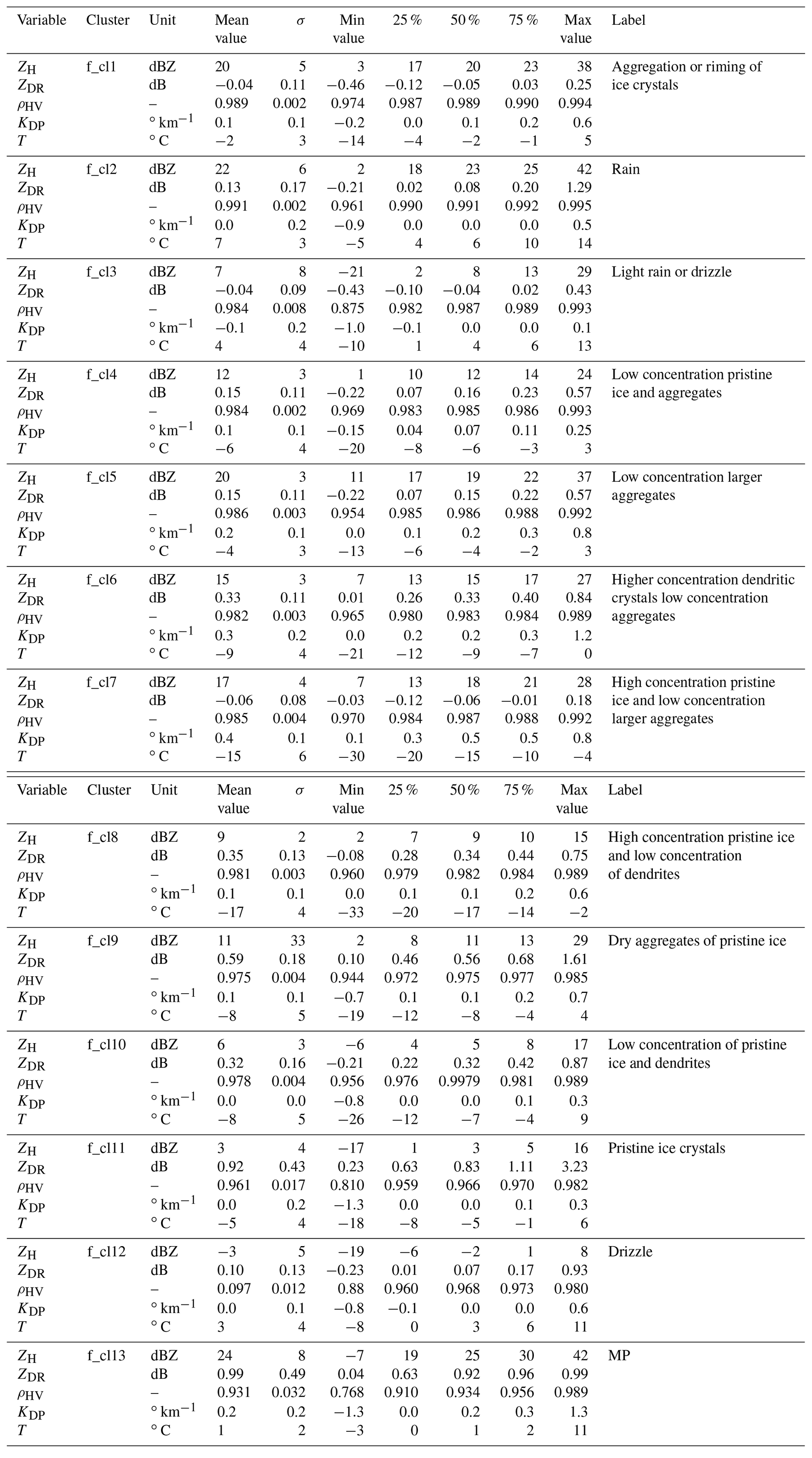

Figure B1The height vs. time format of the final optimal set of active clusters found by the top-down hierarchical clustering for the QVP input data described in Table 1. The observations were made on (a) 1 February 2017, (b) 3 February 2017, (c) 3 March 2017, (d) 22 March 2017, (e) 17 May 2017, (f) 24 January 2018, (g) 13 February 2018 and (h) 14 February 2018. (The hierarchical structure behind the optimal clustering is found in Fig. 4.)
The code can be made available upon request from the corresponding author.
The data are available through the Centre for Environmental Data Analysis (CEDA) archive. The flight data are available at http://catalogue.ceda.ac.uk/uuid/b1c81845ad294f8399f9b564da59c68c (last access: 25 January 2021, FAAM et al., 2017), http://catalogue.ceda.ac.uk/uuid/dbbf8c12f3ad48309829735f7f2e6359 (last access: 25 January 2021, FAAM et al., 2018a), http://catalogue.ceda.ac.uk/uuid/64c9279112bb4e0cadb6adaebf1141eb (last access: 25 January 2021, FAAM et al., 2018b), and http://catalogue.ceda.ac.uk/uuid/25b2a346c6f24032ba746b9dc852ff75 (last access: 25 January 2021, FAAM et al., 2018c). The temperature data are available at https://catalogue.ceda.ac.uk/uuid/f47bc62786394626b665e23b658d385f (last access: 25 January 2021, Met Office, 2016). The NXPol weather radar data are available at https://doi.org/10.5285/ffc9ed384aea471dab35901cf62f70be (Bennett, 2020).
ML conceived the ideas presented herein, implemented the hierarchical algorithm, performed the experiments, and drafted the paper. ML, JC and RRNIII designed the figures and interpreted the results. DD implemented the QVP extraction. JMH processed the temperature data and provided them in the required format for the QVP clustering. LB and DD performed the raw radar data calibration and preprocessing. JC provided the CIP data and its interpretation for the cluster validation part of the study. RRNIII was involved in planning and supervising the work and worked on the paper. All authors discussed the results and contributed to the final article.
The authors declare that they have no conflict of interest.
The authors would like to thank NCAS for support of all scientific activities and, in particular, the FAAM BAe 146 team for collecting the in situ observations and Chilbolton staff for supporting the operations of the NXPol. The authors are grateful to Hannah Price, Chris Reed and Graeme Nott for their help with CIP data processing. Airborne data were obtained using the BAe 146-301 Atmospheric Research Aircraft (ARA) flown by Airtask Ltd and managed by FAAM Airborne Laboratory, jointly operated by UKRI and the University of Leeds. This study also used JASMIN, the UK collaborative data analysis facility.
This research has been supported by the Natural Environment Research Council (grant nos. NE/P012426/1 and NE/S001298/1).
This paper was edited by Gianfranco Vulpiani and reviewed by two anonymous referees.
Abdi, H. and Williams, L. J.: Principal component analysis, WIREs Comp. Stat., 2, 433–459, 2010.
Al-Sakka, H., Boumahmoud, A. A., Fradon, B., Frasier, S. J., and Tabary, P.: A new fuzzy logic hydrometeor classification scheme applied to the French X-, C-, and S-band polarimetric radars, J. Appl. Meteorol. Clim., 52, 2328–2344, 2013.
Aydin, K., Seliga, T. A., and Balaji, V.: Remote sensing of hail with a dual linear polarization radar, J. Appl. Meteorol., 25, 1475–1484, 1986.
Baldini, L. and Gorgucci, E.: Identification of the Melting Layer through Dual-Polarization Radar Measurements at Vertical Incidence, J. Atmos. Ocean. Tech., 23, 829–839, https://doi.org/10.1175/JTECH1884.1, 2006.
Baumgardner, D., Jonsson, H., Dawson, W., O'Connor, D., and Newton, R.: The cloud, aerosol and precipitation spectrometer: a new instrument for cloud investigations, Atmos. Res., 59–60, 251–264, https://doi.org/10.1016/S0169-8095(01)00119-3, 2001.
Baumgardner, D., Abel, S.J., Axisa, D., Cotton, R., Crosier, J., Field, P., Gurganus, C., Heymsfield, A., Korolev, A., Krämer, M., Lawson, P., McFarquhar, G., Ulanowski, Z., and Um, J.: Cloud Ice Properties: In Situ Measurement Challenges, Meteor. Mon., 58, 9.1–9.23, https://doi.org/10.1175/AMSMONOGRAPHS-D-16-0011.1, 2017.
Bechini, R. and Chandrasekar, V.: A Semisupervised Robust Hydrometeor Classification Method for Dual-Polarization Radar Applications, J. Atmos. Ocean. Tech., 32, 22–47, 2015.
Bechini, R., Baldini, L., and Chandrasekar, V.: Polarimetric radar observations in the ice region of precipitating clouds at C-band and X-band radar frequencies, J. Appl. Meteorol. Clim., 52, 1147–1169, https://doi.org/10.1175/JAMC-D-12-055.1, 2013.
Bennett, L.: NCAS mobile X-band radar scan data from 1st November 2016 to 4th June 2018 deployed on long-term observations at the Chilbolton Facility for Atmospheric and Radio Research (CFARR), Hampshire, UK, Centre for Environmental Data Analysis, https://doi.org/10.5285/ffc9ed384aea471dab35901cf62f70be, 2020.
Besic, N., Figueras i Ventura, J., Grazioli, J., Gabella, M., Germann, U., and Berne, A.: Hydrometeor classification through statistical clustering of polarimetric radar measurements: a semi-supervised approach, Atmos. Meas. Tech., 9, 4425–4445, https://doi.org/10.5194/amt-9-4425-2016, 2016.
Besic, N., Gehring, J., Praz, C., Figueras i Ventura, J., Grazioli, J., Gabella, M., Germann, U., and Berne, A.: Unraveling hydrometeor mixtures in polarimetric radar measurements, Atmos. Meas. Tech., 11, 4847–4866, https://doi.org/10.5194/amt-11-4847-2018, 2018.
Bringi, V. N. and Chandrasekar, V. : Polarimetric Doppler Weather Radar: Principles and Applications, Cambridge University Press, UK, 662 pp., 2001.
Bringi, V. N., Chandrasekar, V., Balakrishnan, N., and Zrnić, D. S.: An examination of propagation effects in rainfall on radar measurements at microwave frequencies, J. Atmos. Ocean. Tech., 7, 829–840, 1990.
Crosier, J., Bower, K. N., Choularton, T. W., Westbrook, C. D., Connolly, P. J., Cui, Z. Q., Crawford, I. P., Capes, G. L., Coe, H., Dorsey, J. R., Williams, P. I., Illingworth, A. J., Gallagher, M. W., and Blyth, A. M.: Observations of ice multiplication in a weakly convective cell embedded in supercooled mid-level stratus, Atmos. Chem. Phys., 11, 257–273, https://doi.org/10.5194/acp-11-257-2011, 2011.
Desgraupes, B.: ClusterCrit: Clustering Indices, R Package Version 1.2.3., available at: https://cran.r-project.org/web/packages/clusterCrit/ (last access: 6 September 2017), 2013.
FAAM (Facility for Airborne Atmospheric Measurements), NERC (Natural Environment Research Council), and Met Office: FAAM C013 Instrument Test flight: Airborne atmospheric measurements from core and non-core instrument suites on board the BAE-146 aircraft, Centre for Environmental Data Analysis, available at: http://catalogue.ceda.ac.uk/uuid/b1c81845ad294f8399f9b564da59c68c (last access: 25 January 2021), 2017.
FAAM, NERC, and Met Office: FAAM C076 PICASSO flight: Airborne atmospheric measurements from core and non-core instrument suites on board the BAE-146 aircraft, Centre for Environmental Data Analysis, available at: http://catalogue.ceda.ac.uk/uuid/dbbf8c12f3ad48309829735f7f2e6359 (last access: 25 January 2021), 2018a.
FAAM, NERC, and Met Office: FAAM C081 PICASSO flight: Airborne atmospheric measurements from core and non-core instrument suites on board the BAE-146 aircraft, Centre for Environmental Data Analysis, available at: http://catalogue.ceda.ac.uk/uuid/64c9279112bb4e0cadb6adaebf1141eb (last access: 25 January 2021), 2018b.
FAAM, NERC, and Met Office: FAAM C082 PICASSO flight: Airborne atmospheric measurements from core instrument suite on board the BAE-146 aircraft. Centre for Environmental Data Analysis, available at: http://catalogue.ceda.ac.uk/uuid/25b2a346c6f24032ba746b9dc852ff75 (last access: 25 January 2021), 2018c.
Field, P. R., Heymsfield, A. J., and Bansemer, A.: Shattering and Particle Interarrival Times Measured by Optical Array Probes in Ice Clouds, J. Atmos. Ocean. Tech., 23, 1357–1371, https://doi.org/10.1175/JTECH1922.1, 2006.
Giangrande, S. E. and Ryzhkov, A. V.: Estimation of rainfall based on the results of polarimetric echo classification, J. Appl. Meteorol. Clim., 47, 2445–2462, 2008.
Grazioli, J., Tuia, D., and Berne, A.: Hydrometeor classification from polarimetric radar measurements: a clustering approach, Atmos. Meas. Tech., 8, 149–170, https://doi.org/10.5194/amt-8-149-2015, 2015.
Griffin, E. M., Schuur, T. J., and Ryzhkov, A. V.: A Polarimetric Analysis of Ice Microphysical Processes in Snow, Using Quasi-Vertical Profiles, J. Appl. Meteorol. Clim., 57, 31–50, https://doi.org/10.1175/JAMC-D-17-0033.1, 2018.
Hall, M. P. M., Goddard, J. W., and Cherry, S. M.: Identification of hydrometeors and other targets by dual-polarization radar, Radio Sci., 19, 132–140, 1984.
Hämäläinen, J., Jauhiainen, S., and Kärkkäinen, T.: Comparison of Internal Clustering Validation Indices for Prototype-Based Clustering, Algorithms, 10, 105, https://doi.org/10.3390/a10030105, 2017.
Hancock, R.: Notes on Bayesian Information Criterion Calculation for X-Means Clustering, GitHub, available at: https://github.com/bobhancock/goxmeans/blob/master/doc/BIC_notes.pdf (last access: 25 January 2021), 2012.
Hendry, A. and Antar, Y. M. M.: Precipitation particle identification with centimeter wavelength dual-polarization radars, Radio Sci., 19, 115–122, 1984.
Heymsfield, A. J. and Parrish, J. L.: A Computational Technique for Increasing the Effective Sampling Volume of the PMS Two-Dimensional Particle Size Spectrometer, J. Appl. Meteorol., 17, 1566–1572, https://doi.org/10.1175/1520-0450(1978)017<1566:ACTFIT>2.0.CO;2, 1978.
Johnson, B. T., Petty, G. W., and Skofronick-Jackson, G.: Microwave Properties of Ice-Phase Hydrometeors for Radar and Radiometers: Sensitivity to Model Assumptions, J. Appl. Meteorol. Clim., 51, 2152–2171, https://doi.org/10.1175/JAMC-D-11-0138.1, 2012.
Keat, W. J. and Westbrook, C. D.: Revealing layers of pristine oriented crystals embedded within deep ice clouds using differential reflectivity and the copolar correlation coefficient, J. Geophys. Res.-Atmos., 122, 11737–11759, https://doi.org/10.1002/2017JD026754, 2017.
Korolev, A. V.: Reconstruction of the sizes of spherical particles from their shadow images. Part I: Theoretical considerations, J. Atmos. Ocean. Tech., 24, 376–389, https://doi.org/10.1175/JTECH1980.1, 2007.
Kumjian, M. R., Ryzhkov, A. V., Reeves, H. D., and Schuur, T. J.: A dual-polarization radar signature of hydrometeor refreezing in winter storms, J. Appl. Meteorol. Clim., 52, 2549–2566, 2013.
Kumjian, M. R., Mishra, S., Giangrande, S. E., Toto, T., Ryzhkov, A. V., and Bansemer, A.: Polarimetric radar and aircraft observations of saggy bright bands during MC3E, J. Geophys. Res.-Atmos., 121, 3584–3607, https://doi.org/10.1002/2015JD024446, 2016.
Liu, H. and Chandrasekar, V.: Classification of hydrometeors based on polarimetric measurements: Development of fuzzy logic and neuronfuzzy systems, and in situ verification, J. Atmos. Ocean. Tech., 17, 140–164, 2000.
Met Office: NWP-UKV: Met Office UK Atmospheric High Resolution Model data, Centre for Environmental Data Analysis, date of citation, available at: https://catalogue.ceda.ac.uk/uuid/f47bc62786394626b665e23b658d385f (last access: 25 January 2021), 2016.
Murphy, A. M., Ryzhkov, A., and Zhang, P.: Columnar Vertical Profile (CVP) Methodology for Validating Polarimetric Radar Retrievals in Ice Using In Situ Aircraft Measurements, J. Atmos. Ocean. Tech., 37, 1623–1642, https://doi.org/10.1175/JTECH-D-20-0011.1, 2020.
Neely III, R. R., Bennett, L., Blyth, A., Collier, C., Dufton, D., Groves, J., Walker, D., Walden, C., Bradford, J., Brooks, B., Addison, F. I., Nicol, J., and Pickering, B.: The NCAS mobile dual-polarisation Doppler X-band weather radar (NXPol), Atmos. Meas. Tech., 11, 6481–6494, https://doi.org/10.5194/amt-11-6481-2018, 2018.
Ng, A., Jordan, M., and Weiss, Y.: On spectral clustering: analysis and an algorithm, in: Advances in Neural Information Processing Systems, edited by: Dietterich, T., Becker, S., and Ghahramani, Z., MIT Press, Cambridge, 14, 849–856, 2002.
Niemelä, M., Ayrämo, S., and Kärkkäinen, T.: Comparison of Cluster Validation Indices with Missing Data, in: ESANN 2018 proceedings, European Symposium on Artificial Neural Networks, Computational Intelligence and Machine Learning, Bruges, Belgium, 25–27 April 2018, i6doc.com publ., ISBN 978-287587047-6, available at: http://www.i6doc.com/en/ (last access: 25 January 2021), 2018.
O'Shea, S., Crosier, J., Dorsey, J., Gallagher, L., Schledewitz, W., Bower, K., Schlenczek, O., Borrmann, S., Cotton, R., Westbrook, C., and Ulanowski, Z.: Characterising optical array particle imaging probes: implications for small ice crystal observations, Atmos. Meas. Tech. Discuss. [preprint], https://doi.org/10.5194/amt-2020-265, in review, 2020.
O'Shea, S. J., Crosier, J., Dorsey, J., Schledewitz, W., Crawford, I., Borrmann, S., Cotton, R., and Bansemer, A.: Revisiting particle sizing using greyscale optical array probes: evaluation using laboratory experiments and synthetic data, Atmos. Meas. Tech., 12, 3067–3079, https://doi.org/10.5194/amt-12-3067-2019, 2019.
Pelleg, D. and Moore, A. W.: X-means: extending K-means with efficient estimation of the number of clusters, in: Proceedings of the 17th International Conference on Machine Learning (ICML), Stanford, USA, 727–734, 2000.
Ribaud, J.-F., Machado, L. A. T., and Biscaro, T.: X-band dual-polarization radar-based hydrometeor classification for Brazilian tropical precipitation systems, Atmos. Meas. Tech., 12, 811–837, https://doi.org/10.5194/amt-12-811-2019, 2019.
Roberto, N., Baldini, L., Adirosi, E., Facheris, L., Cuccoli, F., Lupidi, A., and Garzelli, A. A.: A Support Vector Machine Hydrometeor Classification Algorithm for Dual-Polarization Radar, Atmosphere, 8, 134, https://doi.org/10.3390/atmos8080134, 2017.
Ryzhkov, A., Zhang, P., Reeves, H., Kumjian, M., Tschallener, T., Trömel, S., and Simmer, C.: Quasi-vertical profiles–A new way to look at polarimetric radar data, J. Atmos. Ocean. Tech., 33, 551–562, https://doi.org/10.1175/JTECH-D-15-0020.1, 2016.
Ryzhkov, A. V. and Zrnic D. S.: Radar Polarimetry for Weather Observation. Springer Atmospheric Sciences, Springer International Publishing, https://doi.org/10.1007/978-3-030-05093-1, 2019.
Shi, J. and Malik, J.: Normalized cuts and image segmentation, IEEE T. Pattern Anal., 22, 888–905, 2000.
Steinhaus, H.: Sur la division des corps matériels en parties, Bulletin de l'Académie Polonaise des Sciences. Classe 3, 12, 801–804, 1956.
Straka, J. M.: Hydrometeor fields in a supercell storm as deduced from dual-polarization radar, 18th Conf. on Severe Local Storms, San Francisco, Amer. Meteor. Soc., Preprints, 551–554, 1996.
Straka, J. M. and Zrnić, D.S.: An algorithm to deduce hydrometeor types and contents from multiparameter radar data, 26th Int. Conf. on Radar Meteorology, Norman, OK, Amer. Meteor. Soc., Preprints, 513–516, 1993.
Straka, J. M., Zrnić, D. S., and Ryzhkov, A. V.: Bulk hydrometeor classification and quantification using polarimetric radar data: Synthesis of relations, J. Appl. Meteorol., 39, 1341–1372, 2000.
Testud, J., Le Bouar, E., Obligis, E., and Ali-Mehenni, M.: The Rain Profiling Algorithm Applied to Polarimetric Weather Radar, J. Atmos. Ocean. Tech., 17, 332–356, https://doi.org/10.1175/1520-0426(2000)017<0332:TRPAAT>2.0.CO;2, 2000.
Tiira, J. and Moisseev, D.: Unsupervised classification of vertical profiles of dual polarization radar variables, Atmos. Meas. Tech., 13, 1227–1241, https://doi.org/10.5194/amt-13-1227-2020, 2020.
Trömel, S., Kumjian, M., Ryzhkov, A., and Simmer, C.: Backscatter differential phase–Estimation and variability, J. Appl. Meteorol. Clim., 52, 2529–2548, https://doi.org/10.1175/JAMC-D-13-0124.1, 2013.
Trömel, S., Ryzhkov, A., Zhang, P., and Simmer, C.: Investigations of Backscatter Differential Phase in the Melting Layer, J. Appl. Meteorol. Clim., 53, 2344–2359, https://doi.org/10.1175/JAMC-D-14-0050.1, 2014.
Vivekanandan, J., Ellis, S. M., Oye, R., Zrnic, D. S., Ryzhkov, A. V., and Straka, J.: Cloud microphysics retrieval using S-band dual-polarization radar measurements, B. Am. Meteorol. Soc., 80, 381–388, https://doi.org/10.1175/1520-0477(1999)080<0381:CMRUSB>2.0.CO;2, 1999.
von Luxburg, U.: A tutorial on spectral clustering, Stat. Comput., 17, 395–416, 2007.
Wang, H., Ran, Y., Deng, Y., and Wang, X.: Study on deep-learning-based identification of hydrometeors observed by dual polarization Doppler weather radars, EURASIP J. Wirel. Comm., 2017, 179, https://doi.org/10.1186/s13638-017-0965-5, 2017.
Wen, G., Protat, A., May, P. T., Wang, X., and Moran, W.: A cluster-based method for hydrometeor classification using polarimetric variables. Part I: Interpretation and analysis, J. Atmos. Ocean. Tech., 32, 1320–1340, https://doi.org/10.1175/JTECH-D-13-00178.1, 2015.
Wold, S.: Pattern Recognition by Mean of Disjoint Principal Components Models, Pattern Recogn., 8, 127–139, 1976.
- Abstract
- Introduction
- Background of employed methods
- Data and processing
- Clustering of QVPs
- Labelling
- Summary and conclusions
- Appendix A: Polarimetric characteristics of the optimal clusters
- Appendix B: The optimal clusters in eight events
- Code availability
- Data availability
- Author contributions
- Competing interests
- Acknowledgements
- Financial support
- Review statement
- References