XCO₂ estimates from the OCO-2 measurements using a neural network approach

The Orbiting Carbon Observatory (OCO-2) instrument measures high-resolution spectra of the sun's radiance reflected at the earth's surface or scattered in the atmosphere. These spectra are used to estimate the column-averaged dry air mole fraction of CO₂ (XCO₂) and the surface pressure. The official retrieval algorithm (NASA's Atmospheric CO₂ Observations from Space retrievals, ACOS) is a full-physics algorithm and has been extensively evaluated. Here we propose an alternative approach based on an artificial neural network (NN) technique. For training and evaluation, we use as reference estimates (i) the surface pressures from a numerical weather model and (ii) the XCO₂ derived from an atmospheric transport simulation constrained by surface air-sample measurements of CO₂. The NN is trained here using real measurements acquired in nadir mode on cloud-free scenes during even-numbered months and is then evaluated against similar observations during odd-numbered months. The evaluation indicates that the NN retrieves the surface pressure with a root-mean-square error better than 3 hPa and XCO₂ with a 1σ precision of 0.8 ppm. The statistics indicate that the NN trained with a representative set of data allows excellent accuracy that is slightly better than that of the full-physics algorithm. An evaluation against reference spectrophotometer XCO₂ retrievals indicates similar accuracy for the NN and ACOS estimates, with a skill that varies among the various stations. The NN–model differences show spatiotemporal structures that indicate a potential for improving our knowledge of CO₂ fluxes. We finally discuss the pros and cons of using this NN approach for the processing of the data from OCO-2 or other space missions.

1 Introduction

During the past decades, natural fluxes have absorbed about half of the anthropogenic emissions of CO₂ (Knorr, 2009), but there is large uncertainty about the spatial distribution of this sink over time and therefore on the processes that control it. A growing network of high-precision atmospheric CO₂ measurements has been used together with meteorological information to constrain the sources and sinks of CO₂ using a technique known as atmospheric inversion (e.g., Peylin et al., 2013), but the lack of data in large regions of the globe, such as the tropics, does not allow the monitoring of these fluxes with enough space–time resolution. Early attempts to complement this network with satellite retrievals from sensors that were not specifically designed for this purpose were not successful (Chevallier et al., 2005), but a series of dedicated instruments were put into orbit when the Greenhouse Gases Observing Satellite (GOSAT, Yokota et al., 2009) and the second Orbiting Carbon Observatory (OCO-2 Eldering et al., 2017) were launched in 2009 and 2014, respectively. These were still operational at the time of writing. This new and evolving constellation is directly supported by Japanese, US, Chinese, and European space agencies (CEOS Atmospheric Composition Virtual Constellation Greenhouse Gas Team, 2018). All missions have adopted the same CO₂ observation principle that consists of measuring the solar irradiance reflected at the earth's surface in selected spectral bands. Along the double atmospheric path (down-going and up-going), the sunlight is absorbed by atmospheric molecules at specific wavelengths. The resulting absorption lines on the measured spectra make it possible to estimate the amount of gas between the surface and the top of the atmosphere. CO₂ shows many such absorption lines around 1.61 and 2.06 µm that are used to estimate the CO₂ column. Similarly, the oxygen lines around 0.76 µm are used to estimate the surface pressure and can also be used to infer the sunlight atmospheric path, leading to the column-averaged dry air mole fraction of CO₂, referred to as XCO₂ (O'Brien and Rayner, 2002; Crisp et al., 2004).

One main difficulty in the retrieval of XCO₂ from the measured spectra results from the presence of atmospheric particles that scatter light and change its atmospheric path. Accounting for aerosols, in particular, is challenging because aerosols are highly variable in amount and in vertical distribution. Another major difficulty results from modeling errors. The radiative transfer models that are used for the retrieval leave significant residuals between the measured and modeled spectra, even after the XCO₂ and aerosol amount have been inverted for a best fit (Crisp et al., 2012; O'Dell et al., 2018). As a consequence of the various uncertainties in the retrieval process, raw XCO₂ retrievals show significant biases against reference ground-based retrievals (Wunch et al., 2011b, 2017). These biases, together with the comparison against modeling results, led to the development of empirical corrections to the retrieved XCO₂. In the case of the OCO-2 V8r retrievals generated by NASA's Atmospheric CO₂ Observations from Space (ACOS), these corrections amount to roughly half that of the “signal”, i.e., of the difference between the prior and the retrieved XCO₂ (O'Dell et al., 2018).

The limitations in the full-physics retrieval method, despite considerable effort and progress (e.g., O'Dell et al., 2018; Reuter et al., 2017; and Wu et al., 2018 in the case of OCO-2), encourage developing alternative approaches. Here, we want to re-evaluate the potential of an artificial neural network technique (NN) to estimate XCO₂ from the measured spectra. A NN-based technique was already used by Chédin et al. (2003) for a fast retrieval of midtropospheric mean CO₂ concentrations from some meteorological satellite radiometers. These authors trained their NNs on a large ensemble of radiance simulations made using a reference radiation model and assuming diverse atmospheric and surface conditions. NN-based approaches are also commonly used for the retrieval of other species from various high-spectral-resolution satellite radiance measurements because of their computational efficiency (e.g., Hadji-Lazaro et al., 1999).

A NN approach requires a large and representative training dataset. A standard method for problems similar to that discussed here is to use a radiative transfer model and to generate a large ensemble of pseudo-observations based on assumed atmospheric and surface parameters. However, as mentioned above, the radiative transfer models have deficiencies that are rather small, but nevertheless significant with respect to the high-precision objective of the CO₂ measurements. In addition, there may be some wrong assumptions and unknown instrumental defects that are not accounted for in the forward modeling. We thus prefer to avoid using such radiative transfer models and rather base the training on a fully empirical approach (see, e.g., Aires et al., 2005). We use real OCO-2 observations together with collocated estimates of the surface pressure and XCO₂. The retrievals from the NN approach are evaluated against model estimates of surface pressure and XCO₂, as well as observations from the Total Carbon Column Observing Network (TCCON, Wunch et al., 2011a). In the following, Sect. 2 presents the approach while Sect. 3 describes the results. Section 4 discusses the results and the way forward.

2 Data and method

Our NN estimates XCO₂ and the surface pressure from nadir spectra measured by the OCO-2 satellite over land. OCO-2 has eight cross-track footprints (e.g., Eldering et al., 2015), but we only use footprint #4 in the following for simplicity. If successful, the same approach can be applied to all footprints. The focus on nadir measurements here is motivated by the complication introduced by the Doppler effect in glint mode, which is the other pointing mode for OCO-2 routine science operations: the absorption lines affect pixel elements that vary among the spectra. These variations of the position of the absorption line may cause additional difficulty to the NN training. The solar lines in the nadir spectra are also affected by Doppler shifts due to the motion of the earth and satellite relative to the sun, but this concerns a limited set of spectral elements that are affected by the solar (Fraunhofer) lines. The development of a glint-mode NN is therefore left for a future study.

We use spectral samples in the three bands of the instrument (around 0.76, 1.61 and 2.06 µm). They have footprints of ∼3 km² on the ground. In principle, each band is described by 1016 pixel elements, but some are marked as bad either because some of the corresponding detectors have died or because of known temporary or permanent issues. We systematically remove 15 pixel elements that are flagged in about 80 % of the spectra and 478 pixels in the band edges. Conversely, we do not remove the spectra that are affected by the deep solar lines and we let the NN handle these specific features. Because the information in the spectrum is mostly in the relative depth of the absorption lines, and not in their overall amplitude, we normalize each spectrum by a radiance that is representative of the offline values (i.e., the mean of the 90 %–95 % range for each spectrum). This essentially removes the impact of the variations in the surface albedo and in the sun irradiance linked to the solar zenith angle. Other input choices may be attempted in the future.

As input to the NN, we add the observation geometry (sun zenith angle and relative azimuth). The sun zenith angle drives the atmospheric pathlength and is then required for the interpretation of the absorption line depth in terms of atmospheric optical depth. The azimuth was not included in our first attempts, but when later included it led to a significant improvement in the results. Although the NN technique does not allow for a clear physical interpretation, we assume that the information brought by the relative azimuth is linked to the polarization of the molecular scattering contribution to the measurements that varies with the azimuth.

The NN exploits these 2557 input variables to compute two variables only: XCO₂ and the surface pressure. It is structured as a multilayer perceptron (Rumelhart et al., 1988) with one hidden layer of 500 neurons that use a sigmoid activation function. The number of hidden layers is somewhat arbitrary and based on a limited sample of trials. Lower quality estimates were obtained with 50 neurons whereas the training time increased markedly for 1000 neurons and more. The weights of the input variables to the hidden neurons and the weights of the hidden variables to the output variables are adjusted iteratively with the standard Keras library (Keras Team, 2015). Figure A1 in the Appendix illustrates the convergence process. The NN cost function (a.k.a. loss) becomes fairly constant for a test dataset after about 100 iterations, whereas it continues to decrease for the training dataset, indicating an overfitting of the data. The iteration is stopped when there is no decrease of the test loss for 50 iterations. There is a factor of 3 to 4 between the loss of the training dataset and that of the test, which confirms the overfitting of the former.

Note that the NN estimate does not use any a priori information on surface pressure or the CO₂ profile after the training is done. Also, no explicit information is provided on the altitude, location, or time period of the observation. The NN estimates are therefore only driven by the OCO-2 spectrum measurements, together with the observation geometry (sun zenith and relative azimuth). The observation geometry varies with the latitude and the season so that the NN may infer some location information from this input. Conversely, it is the same from one year to the next and, at a given date, for all longitudes. Thus, there is no information on the longitude or the year of observation in the geometry parameters that are provided to the network.

The NN training is based on OCO-2 radiance measurements (V8r) acquired during even-numbered months between January 2015 and August 2018. The 4-year period allows varying the global background CO₂ dry air mole fraction by ∼2 %, as much as typical XCO₂ seasonal variations in the northern extratropics (see, e.g., Fig. 1 of Agustí-Panareda et al., 2019). Our evaluation dataset is based on observations during the odd-numbered months of the same period. In both cases, we make use of XCO₂ estimates and the quality control filters of the ACOS L2Lite V9r products: only observations with xco2_quality_flag = 0 are used. We also consider the warn level, outcome flag and cloud_ flag_idp that are provided in the V8r L2lite and L2Std files. For NN training, we only use the best quality observations, i.e., those with a warn level lower or equal to 2, a cloud_flag of 3 (very clear) and an outcome flag of 1. This choice is based on the evaluation of the surface pressure estimates described below (Fig. 3). This distinction leads to about 131 000 observations for the training. For the evaluation of the NN estimates, we use less restrictive criteria and accept observations with outcome_flag of either 1 or 2, and cloud_flag of 2 or 3. These choices are justified below. The spatial distribution of the observations that are used for the training is shown in Fig. A2 of the Appendix. The training dataset covers most regions of the globe with the exception of South America. The underrepresentation of this subcontinent stems from both the high cloudiness and impact of cosmic rays that leads to missing pixel elements (see below).

For the reference surface pressure (training and evaluation), an obvious choice is the use of numerical weather analyses corrected for the sounding altitude. Indeed, the typical accuracy for surface pressure data is on the order of 1 hPa (Salstein et al., 2008). For convenience, we use the surface pressure that is provided together with the OCO-2 data and is derived from the Goddard Earth Observing System, Version 5, Forward Processing for Instrument Teams (GEOS5-FP-IT) created at the Goddard Space Flight Center Global Modeling and Assimilation Office (Suarez et al., 2008; and Lucchesi et al., 2013). There is no such obvious choice for XCO₂ as there is no global-scale highly accurate dataset of XCO₂ and we thus rely here on best estimates from a modeling approach. We use the CO₂ atmospheric inversion of the Copernicus Atmosphere Monitoring Service (CAMS, http://atmosphere.copernicus.eu, last access: 28 January 2020, Chevallier et al., 2010; version 18r2). This product was released in July 2019 and contributed, e.g., to the Global Carbon Budget 2019 of Friedlingstein et al. (2019). It results from the assimilation of CO₂ surface air-sample measurements in a global atmospheric transport model run at spatial resolution 1.90^∘ in latitude and 3.75^∘ in longitude over the period from 1979–2018 and using the adjoint of this transport model. Neither satellite retrievals nor TCCON observations were used for this modeling. For each OCO-2 observation, XCO₂ is computed from the collocated concentration vertical profile, through a simple integration weighted by the pressure width of the model layers. Note that the model layers use “dry” pressure coordinates so that there is no need for a water vapor correction in the vertical integration. The GEOS5-FP-IT surface pressure and the XCO₂ from CAMS are used both for the training and the evaluation, although using independent datasets (odd- and even-numbered months).

Many measured spectra lack one or several spectral pixels. This is particularly the case over South America, as a consequence of the South Atlantic cosmic ray flux anomaly that impacts the OCO-2 detector in this region. We therefore devised a method to interpolate the spectra and to fill the missing pixels. Our method first sorts all spectral pixels as a function of the measured radiance in a large number of complete measured spectra. The pixel ranks are averaged to generate a rank representative of the full dataset. Then, when a pixel element is missing in a spectrum, we look for its typical rank and we average the radiances of the two pixel elements that have the ranks just above and below. The procedure is applied even when several pixel elements are missing in a spectrum, except when these are successive in the typical ranking. The procedure described here fills the missing elements and the NN can then be applied to the corrected spectrum to estimate the surface pressure and XCO₂.

3 Results

Figure 1 shows a density histogram of the GEOS5 FP-IT surface pressure analysis and of the NN estimate for the evaluation dataset (odd-numbered months). Clearly, there is an excellent agreement between the two over a very wide range of surface pressures. There is no significant bias and the standard deviation is 2.9 hPa. The equivalent ACOS V8r retrieval shows a bias of 1.5 hPa and a standard deviation of 3.4 hPa, slightly larger than that of the NN approach. Note that the ACOS statistics are those of the ACOS retrieval–minus–prior statistics (see Sect. 2). Interpreting them in terms of error is counterintuitive because the Bayesian retrieval is supposed to be better than the prior, but in practice radiation modeling errors lead to a different interpretation (see, e.g., the discussion in Sect. 4.3.4 of O'Dell et al., 2018).

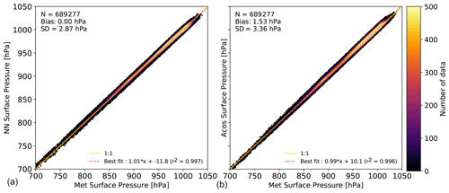
Figure 1 Density histogram of the surface pressure retrieved from the OCO-2 satellite measurements against those derived from GEOS-FP-IT. Panel (a) is for the NN approach while panel (b) is for the ACOS V9r retrieval (using the official bias correction). The figure insets provide the number of data points, the bias, the standard deviation, the equation of the best linear fit, and the correlation. The yellow line is the 1:1 line whereas the red dotted line is the best linear fit.

Both NN and ACOS correlations with GEOS5 FP-IT are very high (0.997 and 0.996) although the best fit shows a very small deviation from the 1:1 line. Interestingly, the best-fit deviations from the 1:1 line are of opposite sign (slopes 0.99 and 1.01). The results of the NN are surprisingly good given the simplicity of the approach and given that the NN estimate does not use any a priori information or ancillary information such as the surface altitude or temperature profile, contrarily to the ACOS estimate. The quality of the NN results for the estimate of the surface pressure is a first demonstration of the potential of the approach. Note that the retrieval accuracy holds over a very large range of surface pressures (the relative variations of XCO₂ are much smaller), although there is some indication of biases for the lowest pressures that are underrepresented in the training dataset. These biases of ≈5 hPa affect the observations over high-elevation surfaces such as the Tibetan Plateau or the US Rocky Mountains.

Figure 2 is similar to Fig. 1 but for XCO₂. There is no significant bias between the NN estimate and the CAMS model, while the standard deviation is 0.84 ppm. The bias-corrected ACOS retrievals show a slight bias against the CAMS model and the standard deviation (1.14 ppm) is larger than that of the NN approach. Note that the statistics given here are affected by CAMS modeling errors that may eventually be corrected with the help of the satellite information. The best fit slope deviations from the 1:1 line are larger than for the surface pressure; the slopes are 0.93 for the NN and 0.87 for ACOS.

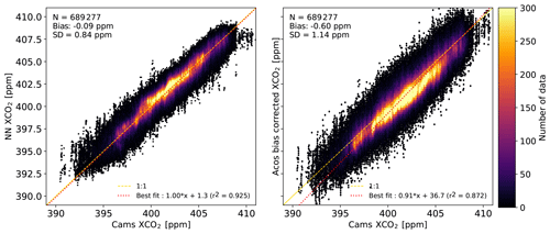
Figure 2 Same as Fig. 1 but for XCO₂. In this case, the reference data are the CAMS v18r2 simulation.

Figures 1 and 2, together with the quantitative assessment of the precision, are given for the observations that are clear according to ACOS (cloud flag = 2 or 3), that have a warn level of 2 or less, that may include missing pixel elements, and that have an outcome flag of 1 or 2. This choice is based on a prior performance analysis. We have analyzed how the performance of the NN approach varies with the quality indicators. For this objective, we have compared the retrieved surface pressure against the value derived from the numerical weather data, as in Fig. 1, and we have evaluated the statistics of their difference as a function of the quality flags. First (figure not shown), there is no significant difference between the cases when the measured spectra are complete and those when one or several missing pixel elements have been interpolated with the method described above. Conversely, the statistics vary with the cloud flag and the warn level, as shown in Fig. 3. We only use the spectra for which an ACOS retrieval is available. Among those, and according to the flag cloud_flag_idp, about 53 % are labeled as “very clear” while 43 % are “probably clear”. The statistics are slightly better for the former than they are for the latter. Conversely, the rather rare “definitely cloudy” and “probably cloudy” show deviations that are significantly larger. This result was highly expected since our NN did not learn how to handle clouds in the spectra. Therefore, all “definitely cloudy” and “probably cloudy” soundings are outside the domain covered by the training dataset. Note also that the observations used here have all been classified as “clear” by ACOS preprocessing. Thus, most OCO-2 observations are not used here and Fig. 3 should not be interpreted as the ability to retrieve the surface pressure in cloudy conditions. Most (78 %) of the observations have a warn level of 0. The deviation statistics increase with the warn level, both in terms of bias and standard deviation. In comparison, the difference in the statistics for an outcome flag of 1 and 2 are small. Besides, more than half of the ACOS retrievals have an outcome flag of 2, which encourages us not to reject those for further use. Based on this analysis, we retain all spectra that are very clear (cloud flag of 2 or 3) and that have a warn level of 2 or less.

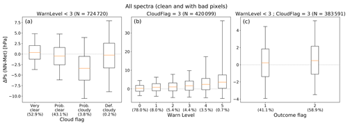
Figure 3 Statistics on the difference between the surface pressure retrieved by the NN approach and those derived from the weather analyses as a function of various quality parameters. In these figures, the red line is the median, the boxes indicate the 25 % and 75 % percentiles, and the whiskers indicate the 5 %–95 % range. Panel (a) shows the statistics as a function of the cloud flag, panel (b) is as a function of the warn level, while panel (c) is as a function of the outcome flag.

We made a figure similar to Fig. 3 but based on the XCO₂ estimates (not shown). Although the results are similar in terms of sign (i.e., increase of the deviations with the warn levels), the signal is not as obvious (there is less relative difference between one warn level and another, or for the various cloud flags). Our interpretation is that the relative accuracy of the surface pressure used as a reference estimate is much better than that of the NN retrieval, whereas the accuracy of the XCO₂ from CAMS is not much better than that of the NN. As a consequence, variations in the accuracy of the NN do not show up as clearly for XCO₂ than they do for the surface pressure.

A standard method to evaluate an algorithm that estimates XCO₂ from spaceborne observation is the comparison of its products against estimates from TCCON retrievals. These estimates use ground-based solar absorption spectra recorded by Fourier transform infrared spectroscopy and have been tuned with airborne in situ profiles (Wunch et al., 2010). To take advantage of the full potential of the TCCON retrievals for the bias correction and validation of the XCO₂ estimates, the OCO-2 platform can be oriented so that the instrument field of view is close to the surface station. The ACOS full-physics algorithm can handle these spectra that are acquired in neither nadir nor glint geometries, but the NN was trained solely on nadir spectra and cannot yet be applied to the observations acquired in target mode. We thus have to rely on nadir measurements acquired in the vicinity of TCCON sites. In the following, we use nadir measurements that are within 5^∘ in longitude and 1.5^∘ in latitude to the TCCON site. The XCO₂ estimates (either from ACOS, the NN, or the model sampled at the OCO-2 measurement location) are averaged for a given overpass. Similarly, we average the TCCON estimates of XCO₂ within 30 min of the satellite overpass. No attempt was made to correct for the different weighting functions of the surface and spaceborne remote sensing estimates. The comparisons are shown in Fig. 4 for each TCCON station listed in Table 1.

Figure 4 Statistics of the differences between the NN retrieval (red), the CAMS model (green) or the bias-corrected ACOS retrievals (blue), and the TCCON retrievals. The boxes indicate the 25 %–75 % percentiles and the median is shown by the horizontal line within the box. The whiskers indicate the 5 %–95 % percentiles. Stations are ordered by increasing latitudes. The numbers below the station name indicate the number of individual observations and coincidence days used for the statistics. The references for the various TCCON observations are provided in Table 1.

Table 1 TCCON stations used in this paper (Fig. 4). The data were obtained from the http://tccondata.org website at during the summer of 2019 (last access: 1 August 2019).

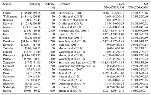
Overall, the biases and standard deviations of the differences to TCCON observations are −0.34 ± 1.40 ppm for the NN, −0.47 ± 1.49 ppm for ACOS and 0.04 ± 1.09 ppm for CAMS. The statistics per station are provided in Table 1. Two stations, Paris and Pasadena, show a large negative bias for both estimates, which may be interpreted as the impact of the city on the atmosphere sampled by the TCCON measurement, while the atmosphere sampled by the distant satellite may be less affected. Conversely, there is no such negative bias for other stations that are located close to large cities, such as Tsukuba, a suburb of the Tokyo Metropolitan area. Zugspitze is rather specific due to its high altitude. The comparison against TCCON indicates that the NN approach performs similarly to ACOS, if not better. The dispersion is larger for one approach versus the other for some stations, while the opposite is true for other stations. Note also that the CAMS model performs better than both satellite retrievals for most stations. This observation provides further justification to the use of this model for training the NN.

The evaluation of the algorithm performance is limited by the distance between the satellite estimate and its surface validation. This is inherent to the use of nadir-only observations that are seldom located close to the TCCON sites. A reduction of the distance results in less coincidences, which leads to a validation dataset of poor representativeness. Note that the CAMS model was sampled at the location of the satellite observations, so that the higher performance of the model versus the satellite products cannot be caused by a higher proximity to the TCCON station.

We now investigate whether the model–minus–NN differences are purely random or contain some spatial or temporal structures. This question is important because if the differences show a random structure there is little hope to use these data to improve the surface fluxes used in the CAMS product. Conversely, if the XCO₂ differences do show some structures, they can be attributed to surface flux errors in the CAMS product that may then be corrected through inverse atmospheric modeling. There is no certainty, however, as a spatial structure in the NN–minus–CAMS difference can also be interpreted as a bias in the satellite estimate.

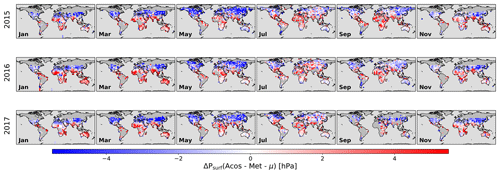
We first show (Fig. 5) the difference between the NN estimates of the surface pressure and the numerical weather analyses. These are monthly maps of the NN-minus-CAMS difference for 3 years of the period at a 5^∘ × 5^∘ resolution. We only present the odd-numbered months as the others were used for the training and therefore do not show any significant differences. There are very clear spatial patterns of a few hPa that are not expected and should be interpreted as a bias in the NN approach. The biases over the high mountains and plateaus have already been mentioned. In addition, positive biases tend to occur in the high latitudes and negative biases toward the tropics. The structures show additional spatial and temporal patterns and are therefore more complex than just a latitude function. The same figure but based on the ACOS retrievals (Fig. A3) displays large-scale structures with different spatial patterns; the surface pressure bias is mostly negative over northern latitudes and positive over low latitudes. A histogram (Fig. 6) of the monthly differences, such as those shown on Fig. 5, confirms that the amplitude of the surface pressure biases is larger with ACOS than it is with the NN. The NN or ACOS surface pressure bias is −0.33 hPa or 1.39 hPa, respectively, and the standard deviation is 2.12 or 2.79 hPa, respectively.

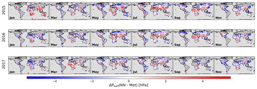
Figure 5 Difference between the NN estimates of the surface pressure and the numerical weather analyses. The differences have been averaged at monthly and spatial 5^∘ × 5^∘ resolutions. The results are shown for 3 years and only for the months that were not used for the training.

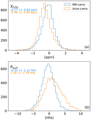
Figure 6 Histogram of the monthly mean differences at 5^∘ resolution (such as those shown in Fig. 5) between the satellite retrievals and the CAMS model: (a) is for XCO₂ while (b) is for the surface pressure. The blue line is for the NN product while the orange line is for ACOS.

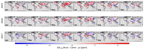
Figure 7 is similar to Fig. 5 but for XCO₂ differences between the NN estimate and the CAMS model. As for the surface pressure, there are clear spatial patterns with amplitudes of 1 to 2 ppm. The question is whether these are mostly linked to monthly biases in the CAMS model or to the NN. The first hypothesis is of course more favorable as it would indicate that the satellite data can bring new information to constrain the surface fluxes. However, the analysis of the surface pressure that shows biases of several hPa suggests that the NN XCO₂ estimate may also show biases with spatially coherent patterns. Interestingly, the patterns vary in time and are not correlated with those of the surface pressure. Further analysis, in particular atmospheric flux inversion, is necessary for a proper interpretation of the NN–CAMS differences.

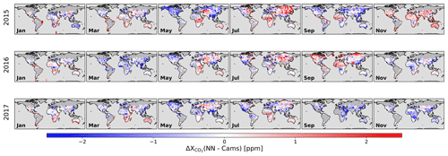
Figure 7 Same as Fig. 5 but for the difference between the XCO₂ estimated by the NN approach and that derived from the CAMS model.

The differences of ACOS estimates to the CAMS model also show patterns of similar amplitude as those in Fig. 7 (Fig. A4). However, there is no clear correspondence between these patterns and those obtained using the NN product. The differences between the satellite products and the CAMS model are small, but these contain the information that may be used to improve our knowledge on the surface fluxes. The absence of a clear correlation between the spatiotemporal pattern from the NN and ACOS approaches indicate that their use would lead to very different corrections on the surface fluxes if used as input of an atmospheric inversion approach. Figure 6a shows the histogram of these monthly mean differences. The histograms are very similar for the two satellite products, although the standard deviation of the difference to the CAMS model is slightly larger for ACOS than it is for the NN approach (0.89 vs. 0.83 ppm).

4 Discussion and conclusion

The use of the same product for the NN training and its evaluation may be seen as a weakness of our analysis. One may argue that the NN has learned from the model and generates an estimate (either the surface pressure or XCO₂) that is not based on the spectra but rather on some prior information. Let us recall that the NN input does not contain any information on the location or date of the observation. This is a strong indication that the information is derived from the spectra as the NN does not “know” the CAMS value that corresponds to the observation location. Yet, the NN input also includes the observation geometry (sun angle and azimuth) that is somewhat correlated with the latitude and day of the year. One may then argue that the NN learns from this indirect information on the observation location and then generates an estimate based on the corresponding CAMS value. However, since the observation geometry is exactly the same from one year to the next, there is no information, direct or indirect, on the observation year in the NN input. Thus, the XCO₂ growth rate that is accurately retrieved by the NN method (see Fig. 7) is necessarily derived from the spectra. A similar argument can be made on the spatial variation across the longitudes.

To further demonstrate that the NN retrieves XCO₂ from the spectra rather than from the prior, we performed an additional experiment. The training is based only on even-numbered months. As a consequence, the prior does not include any direct information on the odd-numbered months. For these months, the best prior estimate is a linear interpolation between the two adjacent even-numbered months. We can then analyze how the NN estimate compares with the CAMS product, which accounts for the true synoptic variability, and a degraded version of CAMS based on a linear interpolation between the two adjacent months. This comparison is shown in Fig. 8. The center figure compares the true CAMS value and that derived from the temporal interpolation. As expected, both are highly correlated (the seasonal cycle and the growth rate are kept in the interpolated values) but nevertheless show a difference standard deviation of 0.89 ppm. This value can be interpreted as the synoptic variability of XCO₂ present in CAMS but not captured in the interpolated product. The comparison of the NN estimate against CAMS (right) and the interpolated CAMS (left) shows significantly better agreement to the former. Thus, the NN product reproduces some XCO₂ variability that is not contained in the training prior. It provides further demonstration that the NN estimates relies on the spectra rather than on the time/space variations of the training dataset.

Figure 8 Scatterplots of XCO₂ estimated by the NN, the CAMS model, and the CAMS model that has been interpolated in time from adjacent months (see text for details). Note that the number of points is less than in Fig. 2 because the edge months could not always be interpolated.

The results shown above indicate that the NN approach allows an estimate of surface pressure and XCO₂ with a precision that is similar or better than that of the operational ACOS algorithm. The lack of independent “truth” data does not allow a full quantification of the product precision and accuracy. However, there are indications that the accuracy on the surface pressure is better than 3 hPa rms, while the precision (standard deviation) of XCO₂ is better than 0.9 ppm. The data used for the XCO₂ product evaluation has its own error that is difficult to disentangle from that of the estimate based on the satellite observation. It may also contain a bias that is propagated to the NN through its training.

One obvious advantage of the NN approach is the speed of the computation, which is several orders of magnitude higher than that of the full-physics algorithm. This is significant given the current reprocessing time of the OCO-2 dataset despite the considerable computing power made available for the mission. It also bears interesting prospects for future XCO₂ imaging missions that will bring even higher data volume (e.g., Pinty et al., 2017).

Another advantage is that the NN approach described in this paper does not require the extensive debias procedure necessary for the ACOS product (O'Dell et al., 2018; Kiel et al., 2019). Per construction, there is no bias between the NN estimates and the dataset used for the NN training. The NN approach therefore requires less effort and fewer resources.

There are, however, a number of drawbacks for the NN approach described in this paper.

One obvious drawback is the use of a CO₂ model simulation in the training while the main purpose of the satellite observation is to improve our current knowledge of atmospheric CO₂ and its surface fluxes. Our argument is that although the CAMS simulation used here has high skill (as demonstrated in Fig. 4), it may have positive or negative XCO₂ biases for some months and some areas. These biases are independent from the measured spectra so that the NN training will aim at average values. As a consequence, the NN product could in principle be of higher quality than the CAMS product, even though the same model has been used as the reference estimate for the training (see, e.g., Aires et al., 2005).

Another drawback of the NN approach is that it does not directly provide its averaging kernel. The averaging kernel vector reports the sensitivity of the retrieved total column to changes in the concentration profile (Connor et al., 1994). It is a combination of physical information (about radiative transfer) and statistical information (about the prior information). It is needed for a proper comparison with 3D atmospheric models (e.g., Chevallier, 2015). When comparing with model simulations, for instance for atmospheric inversion, we may wish to neglect the NN implicit prior information. This hypothesis leads to a homogeneous pressure weighting over the vertical, as this is the product that the NN was trained to simulate. Alternatively, we could decide to neglect the difference in prior information between the NN and the full-physics algorithm and use typical averaging kernels of the latter. A third, more involved option would be to perform a detailed sensitivity study of the NN, based on radiative transfer simulations.

Similarly, the current version of our neural network does not provide a posterior uncertainty. A Monte Carlo approach using various training datasets could be use in the future for such an estimate.

Also, because of the CO₂ growth rate, the developed NN cannot be safely used to process observations that are acquired later than a few weeks after the last data of the training dataset, as the observed CO₂ may then be outside of its range. Therefore, the use of the neural network approach for near real-time applications would require frequent updates of the training phase.

We acknowledge the fact that the NN product evaluated here is not fully independent from the ACOS product. Indeed, we use the cloud flag and the quality diagnostic from ACOS to select the spectra that are of sufficient quality. If we aim for some kind of operational product, there is a need to design a procedure to identify these good quality spectra. One option would be to compare the surface pressure retrieved by the NN to the numerical weather analysis estimate and to reject cases with significant deviations (e.g., differences larger than 3 hPa).

Despite these drawbacks, the results presented here show that a neural network has a large potential for the estimate of XCO₂ from satellite observations, such as those from OCO-2, the forthcoming MicroCarb (Pascal et al., 2017), or the CO₂M constellation (Sierk et al., 2018), which aims to measure anthropogenic emissions. It is rather amazing that a first attempt leads to trueness and precision numbers that are similar or better than those of the full-physics algorithm. There are several paths to improvement. One is to provide the NN with some ancillary information such as the surface altitude or a proxy of the atmospheric temperature. Another is to train the NN with model estimates (such as those of CAMS used here) but that have been better sampled for their assumed precision, for instance through a multimodel evaluation. Also, one could train the NN with observations acquired during a few days of each month, rather than the even-numbered months as done here, so that the evaluation dataset would provide a better evaluation of the seasonal cycle.

Our next objective is to attempt a similar NN approach for the measurements that were acquired in the glint mode. As explained above, the glint observations may be more difficult to reproduce by the NN than those acquired in the nadir mode. However, we were very much surprised by the performance of the NN with the nadir data and cannot preclude being surprised again. Finally, we shall analyze the spatial structure of the NN retrievals in regions that are expected to be homogeneous and in regions where structures of anthropogenic origin are expected (e.g., Nassar et al., 2017; Reuter et al., 2019).

Appendix A

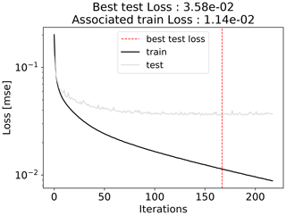
Figure A1 Illustration of the iterative convergence of the NN during its training. The loss is an indicator of the difference between the NN estimate and the dataset. One dataset is used for the best estimate of the NN weights whereas another independent one is used for the evaluation of the NN capability. The NN is stopped when there is no further reduction of the loss for the test dataset for 50 iterations. The weights for the NN are those obtained for the lowest loss of the test dataset (iteration 167 on the figure).

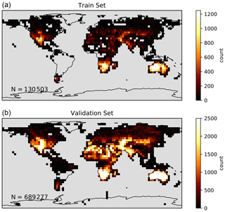
Figure A2 Spatial density of the observations that were used for the training (a) and validation (b) processes.

Figure A3 Same as Fig. 5 but for the surface pressure retrieved by the ACOS algorithm. The mean bias over the full period (μ) is removed so that the differences are centered on zero.

Figure A4 Same as Fig. 7 but for the XCO₂ retrieved by the ACOS algorithm. The mean bias over the full period (μ) is removed so that the differences are centered on zero.