Validation of pure rotational Raman temperature data from the Raman Lidar for Meteorological Observations (RALMO) at Payerne

The Raman Lidar for Meteorological Observations (RALMO) is operated at the MeteoSwiss station of Payerne (Switzerland) and provides, amongst other products, continuous measurements of temperature since 2010. The temperature profiles are retrieved from the pure rotational Raman (PRR) signals detected around the 355 nm Cabannes line. The transmitter and receiver systems of RALMO are described in detail, and the reception and acquisition units of the PRR channels are thoroughly characterized. The FastCom P7888 card used to acquire the PRR signal, the calculation of the dead time and the desaturation procedure are also presented. The temperature profiles retrieved from RALMO PRR data during the period going from July 2017 to the end of December 2018 have been validated against two reference operational radiosounding systems (ORSs) co-located with RALMO, i.e. the Meteolabor SRS-C50 and the Vaisala RS41. The ORSs have also served to perform the calibration of the RALMO temperature during the validation period. The maximum bias (ΔT_max), mean bias (μ) and mean standard deviation (σ) of RALMO temperature T_ral with respect to the reference ORS, T_ors, are used to characterize the accuracy and precision of T_ral along the troposphere. The daytime statistics provide information essentially about the lower troposphere due to lower signal-to-noise ratio. The ΔT_max, μ and σ of the differences $\mathrm{\Delta }T=T_{\mathrm{ral}}-T_{\mathrm{ors}}$ are, respectively, 0.28, 0.02±0.1 and 0.62±0.03 K. The nighttime statistics provide information for the entire troposphere and yield ΔT_max=0.29 K, $\mathit{\mu }=\mathrm{0.05}\pm \mathrm{0.34}$ K and $\mathit{\sigma }=\mathrm{0.66}\pm \mathrm{0.06}$ K. The small ΔT_max, μ and σ values obtained for both daytime and nighttime comparisons indicate the high stability of RALMO that has been calibrated only seven times over 18 months. The retrieval method can correct for the largest sources of correlated and uncorrelated errors, e.g. signal noise, dead time of the acquisition system and solar background. Especially the solar radiation (scattered into the field of view from the zenith angle Φ) affects the quality of PRR signals and represents a source of systematic error for the retrieved temperature. An imperfect subtraction of the background from the daytime PRR profiles induces a bias of up to 2 K at all heights. An empirical correction f(Φ) ranging from 0.99 to 1 has therefore been applied to the mean background of the PRR signals to remove the bias. The correction function f(Φ) has been validated against the numerical weather prediction model COSMO (Consortium for Small-scale Modelling), suggesting that f(Φ) does not introduce any additional source of systematic or random error to T_ral. A seasonality study has been performed to help with understanding if the overall daytime and nighttime zero bias hides seasonal non-zero biases that cancel out when combined in the full dataset.

1 Introduction

Continuous measurements of tropospheric temperature are essential for numerous meteorological applications and in particular for numerical weather predictions, for satellite calibration and validation applications (Stiller et al., 2012; Wing et al., 2018), and for the understanding of climate change. Co-located temperature and humidity measurements allow us to calculate the relative humidity, a parameter playing a key role in several thermodynamic processes, such as the hygroscopic growth of condensation nuclei, fog and cloud formation. When considering the thermodynamic processes occurring within a stagnant air mass, a strong increase in relative humidity is often a precursor of fog, while the onset of supersaturation is linked to a consolidated radiation fog or a cloud forming at the top of a convective layer. Another important thermodynamic parameter is the convective available potential energy (CAPE); CAPE is directly related to the temperature difference between two layers in the atmosphere. The knowledge of temperature as a function of altitude allows us to monitor the atmospheric thermodynamic stability and to diagnose and forecast the onset and intensity of a thunderstorm. Despite its importance in all these processes, the atmospheric temperature is still undersampled in the lower troposphere where the traditional and well-established observing systems (e.g. radiosounding, Aircraft Meteorological DAta Relay (AMDAR), MODE-S (Selective) EHS (enhanced surveillance), satellites) do not provide continuous measurements. A vertical profile of temperature in the troposphere can be measured efficiently by ground-based remote sensing instrumentation; unlike other technologies, remote sensing is best suited to operate continuously and to satisfy real-time data delivery requirements. Moreover, remote sensing instruments operating continuously for many years ensure long time series of data, which are fundamental for climatology studies.

This study focuses on the measurement of the atmospheric temperature done by a light detection and ranging (lidar) instrument. Best known methodologies to retrieve temperature profiles using a lidar can be split into four groups of techniques: the differential absorption lidar (DIAL), the high spectral resolution lidar (HSRL), the Rayleigh technique and the Raman technique (Wulfmeyer et al., 2015, and references therein). Measurements with DIAL are based on the dependency of the molecular absorption on the atmospheric temperature; namely, oxygen molecules with their constant mixing ratio in the dry atmosphere are used as targets by DIAL to retrieve the temperature profile (Behrendt, 2005; Hua et al., 2005). The HSRL technique uses the Doppler frequency shifts produced when photons are scattered from molecules in random thermal motion; the temperature dependence of the shape of the Cabannes line is used directly for temperature measurements (Theopold and Bösenberg, 1993; Wulfmeyer and Bösenberg, 1998; Bösenberg, 1998). The Rayleigh method is based on the assumption that measured photon-count profiles are proportional to the atmospheric mass-density profile in an atmosphere that behaves like an ideal gas and that is in hydrostatic equilibrium. The mass-density profile is used to determine the absolute temperature profile (Hauchecorne et al., 1991; Alpers et al., 2004; Argall, 2007). The pure rotational Raman (PRR) method relies on the dependence of the rotational spectrum on atmospheric temperature (Cooney, 1972; Vaughan et al., 1993; Balin et al., 2004; Behrendt et al., 2004; Di Girolamo et al., 2004; Achtert et al., 2013; Zuev et al., 2017). A combination of the Rayleigh and Raman methods is also possible and allows us to extend significantly the atmospheric region where the temperature is retrieved (Li et al., 2016; Gerding et al., 2008). The four methods have the common objective to produce a temperature profile as close as possible to the true atmospheric status. In the attempt to do that, a reference must be used to calibrate the lidar temperature and calculate the related uncertainty. Trustworthy references can be provided by co-located radiosondes, satellites or numerical models. A co-located radiosounding system (RS) can act as reference to calibrate and monitor the stability of a lidar system over long periods of time (Newsom et al., 2013). Our study presents a characterization of the RSs in use at Payerne and their validation with respect to the Vaisala RS92 certified by the Global Climate Observing System (GCOS) Reference Upper-Air Network (GRUAN). Assimilation experiments using validated Raman lidar temperature profiles have been performed, among others, by Adam et al. (2016) and Leuenberger et al. (2020). Both studies highlight the great potential of Raman lidar to improve numerical weather prediction (NWP) models through data assimilation (DA).

In this study we characterize and validate Raman Lidar for Meteorological Observations (RALMO) temperature profiles and demonstrate the high stability of the system. The paper is organized as follows. In Sect. 2 we establish the quality of the reference radiosonde datasets. The lidar system is described in detail in Sect. 3 followed by a thorough uncertainty budget estimation in Sect. 4. In that section all contributions to the total error are quantified and taken into account (dead-time correction, background correction, photon-counting error, calibration error). In Sects. 5 and 6 we present the statistics of the comparison between lidar and radiosondes. In Sect. 5 we present the statistical analysis of the $\mathrm{\Delta }T=T_{\mathrm{ral}}-T_{\mathrm{ors}}$ dataset, and we analyse the possible causes of μ and σ over the period July 2017–December 2018. An additional statistical study has been performed by splitting the ΔT dataset into seasons to investigate the effect of solar background and its correction function f(Φ) on the retrieved temperature profiles in terms of μ and σ (Sect. 6). The maximum (ΔT_max) and mean bias (μ) of the difference (ΔT) of the lidar temperature profiles with respect to the temporally and spatially co-located radiosonde profiles represent the systematic uncertainty of the lidar temperature. The standard deviation of all differences ΔT over the entire dataset yields the random uncertainty (σ) of the lidar temperature.

2 Validation of the reference radiosounding systems

In the framework of the operational radiosonde flight programme, the operational radiosonde is launched twice daily at Payerne at 11:00 and 23:00 UTC (in order to reach 100 hPa by 00:00 and 12:00 UTC) and provides profiles of humidity (q), temperature (T), pressure (P) and wind (u). In addition to the operational programme, MeteoSwiss is part of the Global Climate Observing System (GCOS) Reference Upper-Air Network (GRUAN) since 2012 with the Vaisala sonde RS92. In the framework of GRUAN, MeteoSwiss has launched from the aerological station of Payerne more than 300 RS92 sondes between 2012 and 2019, contributing significantly to its characterization (metadata, correction algorithms and uncertainty calculation) and to its GRUAN certification (Dirksen et al., 2014; Bodeker and Kremser, 2015). Before being part of GRUAN and since 2005, MeteoSwiss has used the RS92 sonde as working standard in the framework of the quality assurance programme of the different versions of the Meteolabor Swiss radiosonde (SRS). Different versions of the SRS systems were operated at Payerne since 1990, starting from the analogue SRS-400 (from 1990 to 2011) and developing to the digital sondes SRS-C34 and C50. Starting from 2012, different versions of the SRS-C34 and SRS-C50 have been compared to RS92 in the framework of GRUAN. In 2014, the Vaisala RS41 (Dirksen et al., 2020) was added to the GRUAN programme where it performed numerous multi-payload flights with RS92 and the SRS carried under the same balloon.

During the studied period, two different operational radiosounding systems (ORSs) have been launched regularly at 11:00 and 23:00 UTC: the SRS-C50 (February 2017–March 2018) and the Vaisala RS41 (March–December 2018). Thanks to the multi-sensor flights performed with the SRS-C50, the Vaisala RS41 and the Vaisala RS92, the SRS-C50 and RS41 have been validated by the GRUAN-certified RS92. Figures 1 and 2 show the statistical biases of RS41 and SRS-C50 with respect to the reference RS92 as a function of height for the day- and nighttime launches. The differences have been co-added into altitude boxes of 2 km, and the profiles have been sampled every 30 s starting from 15 s after launch. The boxes in the plots have boundaries at the 25th and 75th percentiles and are centred (black dot in each box) in the mean value bias.

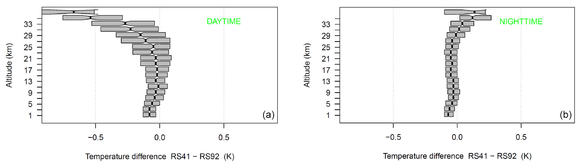
Figure 1 Temperature deviation of RS41 with respect to RS92 calculated from the GRUAN multi-payload flights dataset during June 2015–December 2018. The boxes are centred in the mean bias and span the 25th–75th percentile range. Statistics are based on 58 flights at 11:00 UTC (a) and 59 flights at 23:00 UTC (b).

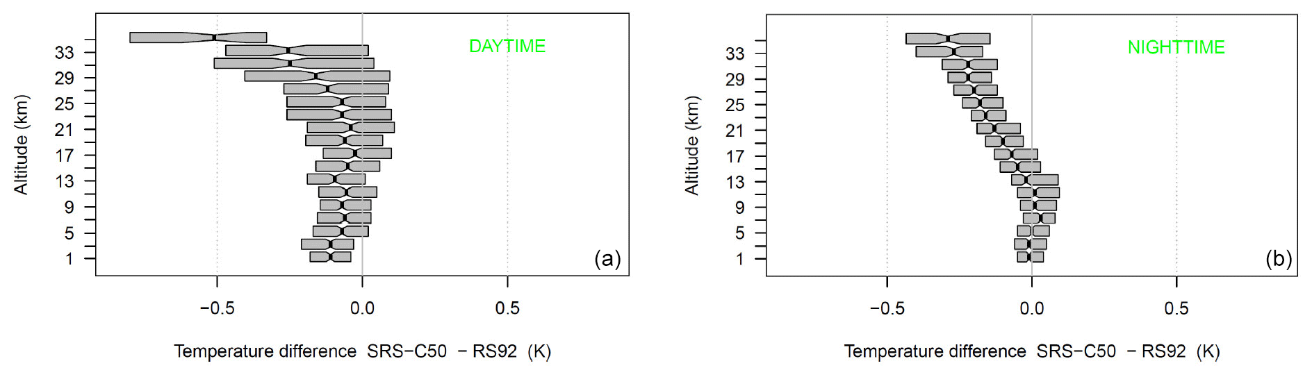
Figure 2 Temperature deviation of SRS-C50 with respect to RS92 calculated from the GRUAN multi-payload flights dataset during February–December 2018. The boxes are centred in the mean bias and span the 25th–75th percentile range. Statistics are based on 25 flights at 11:00 UTC (a) and 26 flights at 23:00 UTC (b).

The RS41 and SRS-C50 show an overall negative bias during both day and night never exceeding −0.1 K along the whole troposphere. Only in the mid-stratosphere, above 30 km, does the daytime biases reach −0.5 K. In the framework of our study, the region of interest for the temperature profiles measured by RALMO is the troposphere and, more rarely, the UTLS (upper troposphere and lower stratosphere, ∼0–14 km). In this region, as the statistics show, the two ORSs perform very well. For the daytime comparisons (11:00 UTC), the mean bias of RS41 over the region 0–14 km is $-\mathrm{0.05}\pm \mathrm{0.03}$ K with a mean standard deviation of 0.15±0.05 K. For the nighttime comparisons (23:00 UTC), the mean bias of RS41 over the region 0–14 km is $-\mathrm{0.05}\pm \mathrm{0.02}$ K with a mean standard deviation of 0.11±0.06 K. The statistics of SRS-C50 for daytime (11:00 UTC) show a mean bias over the region 0–14 km of $-\mathrm{0.08}\pm \mathrm{0.02}$ K and a mean standard deviation of 0.19±0.09 K. For the nighttime comparisons (23:00 UTC), the mean bias of SRS-C50 over the region 0–14 km is $-\mathrm{0.01}\pm \mathrm{0.02}$ K with a mean standard deviation of 0.13±0.04 K.

The comparisons with RS92 show that for both ORSs the daytime differences undergo a larger variability along the 0–14 km vertical range compared to the nighttime statistics. The main reason for the larger variability is that, during the daytime flights, RS92 and the two ORSs undergo different exposures to the solar radiation, which causes a different response of the thermocouple sensors. The effect on the thermocouple becomes larger with altitude as the solar radiation increases with height. All RSs are corrected by the manufacturer for the effects of solar radiation on the thermocouple sensors. However, different manufacturers use different radiation corrections, which contributes to the statistical broadening of the differences at all levels. The overall (11:00 and 23:00 UTC) performance of the two ORSs in terms of bias with respect to the reference RS92 is summarized in Fig. 3. The distribution and mean value of the differences confirm that in the first 15 km the two ORSs remain well below the −0.1 K bias. The RS41 shows closer values to RS92 than SRS-C50 especially in the stratosphere. The better statistics of RS41 should be interpreted also in light of the fact that RS92 and RS41 are both manufactured by Vaisala.

Figure 3 Overall temperature deviations at 11:00 and 23:00 UTC of RS41 (a) and SRS-C50 (b) with respect to the reference sonde RS92. The interpretation of the graphics is the same as for the previous figures.

3 The Raman Lidar for Meteorological Observations – RALMO

RALMO was designed and built by the École Polytechnique Fédérale de Lausanne (EPFL) in collaboration with MeteoSwiss. After its installation at the MeteoSwiss station of Payerne (46^∘48.0^′ N, 6^∘56.0^′ E; 491 m a.s.l.) in 2007 it has provided profiles of q, T and aerosol backscatter (β) in the troposphere and lower stratosphere almost uninterruptedly since 2008 (Brocard et al., 2013; Dinoev et al., 2013). The T data during the 2008–2010 period are unexploited due to low quality of the analogue channel. RALMO has been designed to achieve a measurement precision better than 10 % for q and 0.5 K for T with a 30 min integration time and to reach at least 5 km during daytime and 7 km during nighttime in clear-sky conditions. RALMO uses high-energy emission, narrow field of view of the receiver and a narrowband detection to achieve the required daytime performance. The data acquisition software has been developed to ensure autonomous operation of the system and real-time data availability. RALMO's frequency-tripled Nd:YAG laser emits 400 mJ per pulse at 30 Hz and at 355 nm. A beam expander expands the beam's diameter to 14 cm and reduces the beam divergence to 0.09±0.02 mrad. The returned signal is an envelope of the 355 nm elastic- and Raman-backscattered signals, i.e. PRR, water vapour, oxygen, nitrogen and Rayleigh. Next, the Raman lidar equation (RLE) for the PRR signal is presented along with the detailed description of how RALMO selects the high and low quantum-shifted wavelengths used in the RLE to retrieve the temperature.

3.1 Pure rotational Raman temperature

Raman lidar measurements of the atmospheric temperature rely on the interaction between the probing electromagnetic signal at wavelength (λ) emitted by the lidar and the molecules of O₂ and N₂ encountered along the probing path. In addition to the Rayleigh light backscattered by the aerosols and molecules at the same frequency as the incident light, the O₂ and N₂ molecules return a frequency-shifted Raman signal back to the lidar's receiver. The Raman-backscattered signal is shifted in frequency due to the rotational and vibrational Raman effect. In this study only the pure-rotational part of the spectrum around the Rayleigh frequency (Cabannes line) is detected by RALMO and analysed (Fig. 4).

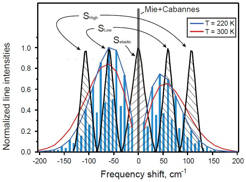
Figure 4 Temperature dependence of the Stokes and anti-Stokes pure rotational Raman spectrum of N₂ calculated at 220 and 300 K. The intensity of the spectral lines are in normalized relative units. The frequency shift on the x axis refers to a laser's wavelength of 355 nm. The total intensity of the high and low quantum-shifted PRR channels is the summation of the single line intensities underneath the bell-shaped black curves.

The Raman lidar equation, RLE, yields the intensity of the PRR signal S_PRR:

$$\begin{array}{}\text{(1)}& \begin{array}{rl}{S}_{\mathrm{PRR}}\left(z\right)& ={\displaystyle \frac{C}{z^{\mathrm{2}}}}O\left(z\right)n\left(z\right){\mathrm{\Gamma }}_{\mathrm{atm}}^{\mathrm{2}}\left(z\right)\\ & \left(\sum _{i={\mathrm{O}}_{\mathrm{2}},{\mathrm{N}}_{\mathrm{2}}}\sum _{J_i}\mathit{\tau }\left(J_i\right){\mathit{\eta }}_i{\left({\displaystyle \frac{\mathrm{d}\mathit{\sigma }}{\mathrm{d}\mathrm{\Omega }}}\right)}_{\mathrm{\Pi }}^i\left(J_i\right)\right)+B.\end{array}\end{array}$$

The received S_PRR signal measured over time t is a function of the altitude z; C is the lidar constant; O(z) is the geometrical overlap between the emitted laser and the receiver's field of view; n(z) is the number density of the air; Γ_atm(z) is the atmospheric transmission; τ(J_i) is the transmission of the receiver for each PRR line J_i; η_i is the volume mixing ratio of nitrogen and oxygen; $\left(\frac{\mathrm{d}\mathit{\sigma }}{\mathrm{d}\mathrm{\Omega }}{)}_{\mathrm{\Pi }}^i\right(J_i)$ is the differential Raman cross section for each PRR line J_i; and B is the background of the measured signal. Air mainly contains oxygen and nitrogen (≈99 %) whose ratio remains fairly constant in the first 80 km of atmosphere, so η_i can be regarded as a constant in Eq. (1). The lidar constant C depends on the overall efficiency of the transceiver (transmitter and receiver) system including the photomultiplier tube (PMT) efficiency, on the area of the telescope and on the signal's intensity. The full expression of the differential Raman cross section for single lines of the PRR spectrum can be found in the reference book chapter by Behrendt (2005).

3.2 Temperature polychromator of RALMO

The two-stage temperature polychromator, hereafter referred to as PRR polychromator, represents the core of the signal selection. The PRR polychromator separates several pure rotational Raman spectral lines and isolates elastic scattering consisting of Rayleigh and Mie lines (Cabannes line).

The PRR signal from the O₂ and N₂ atmospheric molecules is collected by four parabolic, high-efficiency reflecting mirrors each one with a diameter of 30 cm. The mirrors have a dielectric reflection coating with R>99 % for the vibrational Raman wavelengths and R>96 % for the elastic and pure rotational Raman for both cross- and parallel-polarized light. Nine-degree-tilted Semrock RazorEdge filters (REFs) are installed just below the focal points of two of the four mirrors (left of Fig. 5). The REFs are long-wavelength pass filters and have a cut-off wavelength at 364 nm (right of Fig. 5). The ro-vibrational Raman scattering from the atmospheric H₂O, O₂ and N₂ molecules is transmitted by the REF onto the optic fibres placed above the REF at the exact focal distance of the parabolic mirrors. The elastic (Rayleigh and Mie) and PRR scattering are reflected by the tilted REF onto 0.4 mm optic fibres and transmitted to the PRR polychromator.

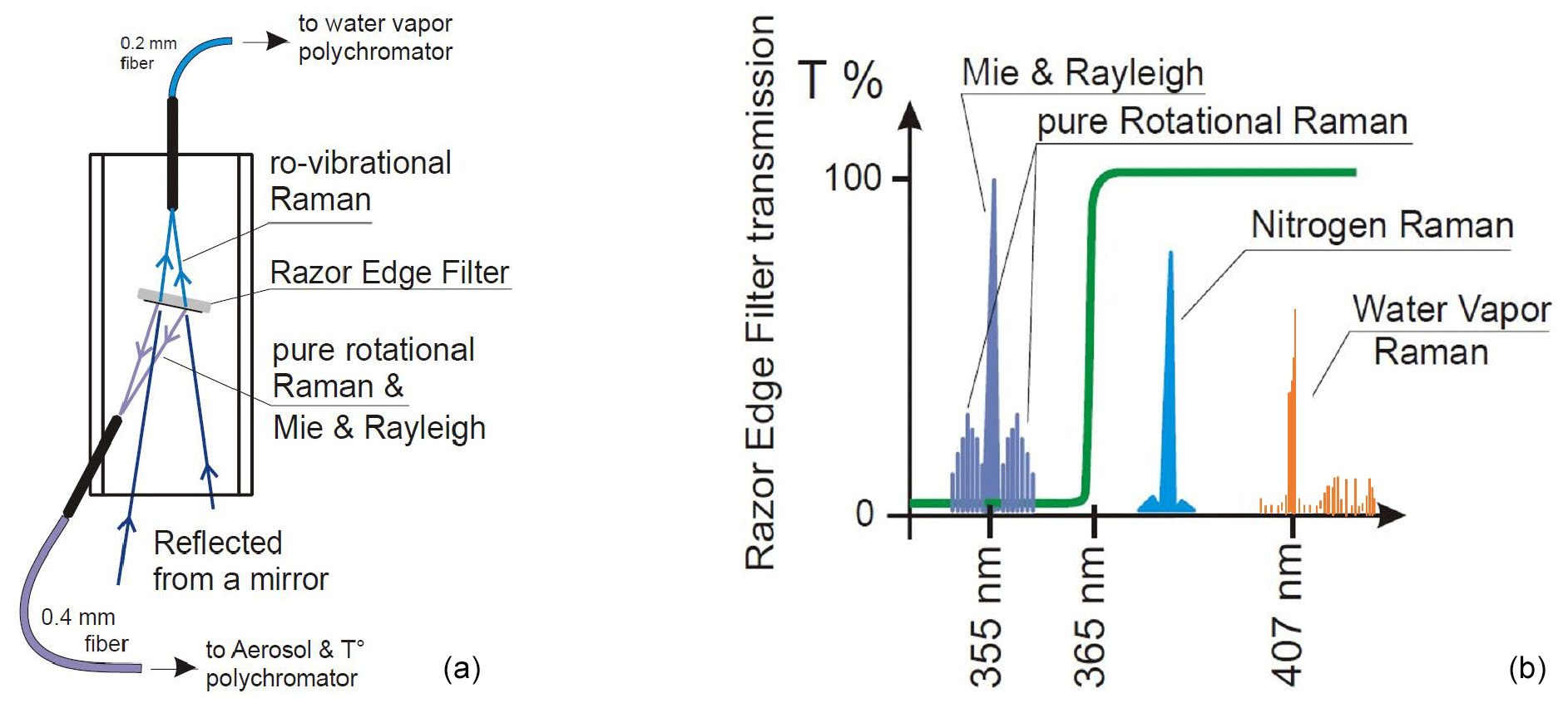
Figure 5 (a) Telescopic mirrors, RazorEdge filter and optic fibres. (b) The REF cut-off frequency applied to the 355 nm Raman spectrum.

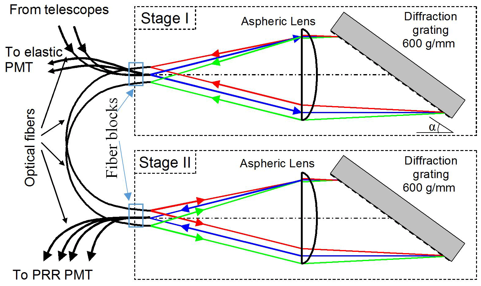
The two optic fibres transmitting the PRR and the elastic signals enter the temperature polychromator through the first fibre's block shown in Fig. 6. The fibres are fixed into the fibre's block, ensuring no or negligible temperature and mechanical-induced drifts of the fibre alignment with respect to the other optical elements inside the polychromator (detailed in Fig. 7). The outline of the two fibre block's Cartesian coordinates system in Fig. 6 shows the position of the input, output and intermediate fibres (from stage 1 to stage 2) as a function of their abscissa–ordinate, x–y, positions. At x=21.5 mm, the input fibres, coming from the mirrors, are located at y=20 mm and y=24 mm; the output “elastic” fibres are located at y=18 mm and y=22 mm. The two output elastic signals are then transmitted through the fibres and combined together just before entering the PMT installed outside the polychromator's box (PMT R12421P, Hamamatsu). The two input fibres transmit the PRR and the elastic signals onto an aspheric lens with focal length of 300 mm and diameter of 150 mm. The two signals are then transmitted through the lens onto a reflective holographic diffraction grating with groove density of 600 grooves mm⁻¹ oriented at a diffraction angle of 48.15^∘ with respect to the axis of the lenses in a Littrow configuration. The two input signals (one from each mirror) are diffracted by the grating polychromator and separated into high and low quantum number lines from both Stokes and anti-Stokes parts of the Raman-shifted spectrum. Two groups of four spectral lines are then diffracted, i.e. $J_{\mathrm{high}}^{\mathrm{Stokes}}$, $J_{\mathrm{high}}^{\mathrm{anti}\text{-}\mathrm{Stokes}}$, $J_{\mathrm{low}}^{\mathrm{Stokes}}$ and $J_{\mathrm{low}}^{\mathrm{anti}\text{-}\mathrm{Stokes}}$.

Table 1 Theoretical polychromator efficiencies (ξ) for the nitrogen PRR lines at wavelengths λ.

The theoretical polychromator efficiencies ξ (ξ∈ [0–1]) for the nitrogen and oxygen PRR lines $J_{\mathrm{high}}^{\mathrm{Stokes}}$, $J_{\mathrm{high}}^{\mathrm{anti}\text{-}\mathrm{Stokes}}$, $J_{\mathrm{low}}^{\mathrm{Stokes}}$ and $J_{\mathrm{low}}^{\mathrm{anti}\text{-}\mathrm{Stokes}}$ are shown in Tables 1 and 2, respectively. The low and high quantum-number signals, J_low and J_high, Raman-backscattered by the nitrogen molecules are diffracted by the polychromator most efficiently at lines with quantum number n=6 ($J_{\mathrm{low}}^{\mathrm{anti}\text{-}\mathrm{Stokes}}$, λ=353.97 nm, $J_{\mathrm{low}}^{\mathrm{Stokes}}$, λ=355.47 nm) and n=12 ($J_{\mathrm{high}}^{\mathrm{anti}\text{-}\mathrm{Stokes}}$, λ=353.37 nm, $J_{\mathrm{high}}^{\mathrm{Stokes}}$, λ=356.07 nm). Similarly to the nitrogen, the PRR signals backscattered by the oxygen molecules are diffracted by the polychromator most efficiently at lines with quantum number n=9 ($J_{\mathrm{low}}^{\mathrm{anti}\text{-}\mathrm{Stokes}}$, λ=353.96 nm, $J_{\mathrm{low}}^{\mathrm{Stokes}}$, λ=355.48 nm) and n=17 ($J_{\mathrm{high}}^{\mathrm{anti}\text{-}\mathrm{Stokes}}$, λ=353.38 nm, $J_{\mathrm{high}}^{\mathrm{Stokes}}$, λ=356.06 nm).

Table 2 Theoretical polychromator efficiencies (ξ) for the oxygen PRR lines at wavelengths λ.

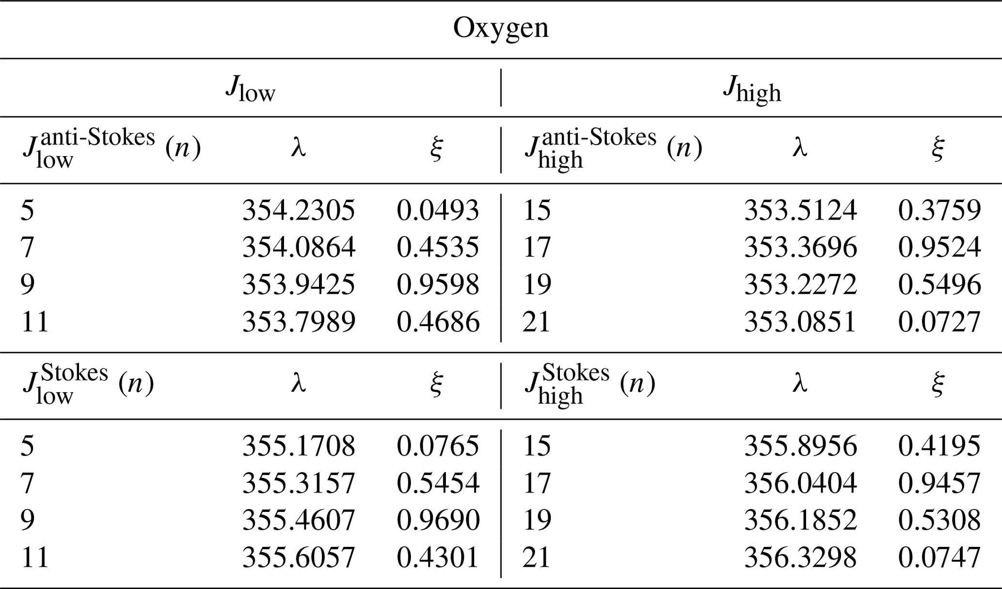
Signals J_low and J_high are sums of the respective Stokes and anti-Stokes lines for nitrogen and oxygen. The eight J signals diffracted by the polychromator are then refocused by the aspheric lens onto the intermediate fibres positioned at the y ordinates y=18 mm and y=22 mm and at the x abscissae x=18.93 mm, x=20.075 mm, x=22.925 mm and x=24.07 mm.

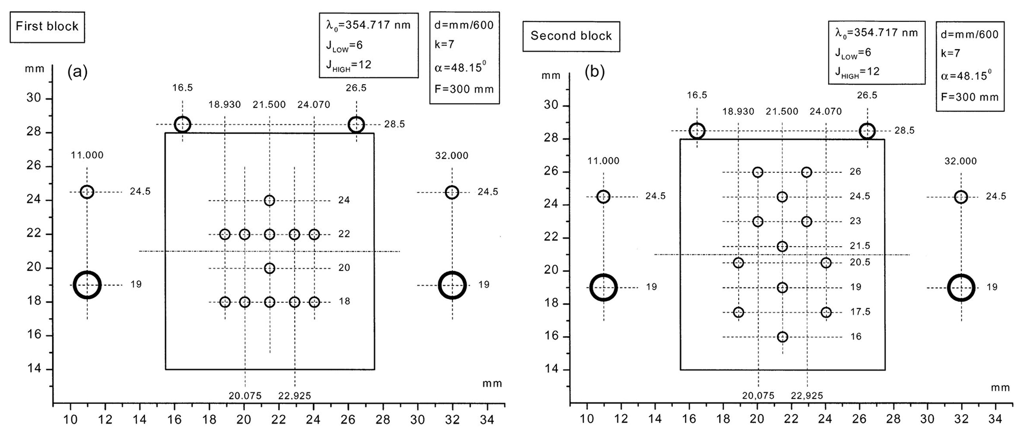
Figure 6 The outline of the two fibres' blocks shows the positions of the input, output and intermediate (from stage 1 to stage 2) fibres as a function of the abscissa–ordinate, x–y Cartesian coordinates. (a) Two optic fibres transmitting the PRR and the elastic signals enter the temperature polychromator through the first fibre's block. (b) The eight Stokes and anti-Stokes J signals are transmitted through the intermediate fibres into the second fibre's block. The eight J signals are recombined by the diffraction grating polychromator into two groups of total J signals (J_high and J_low) and sent to the output fibres. Holes shown outside the fibre's block are not fibre holders.

The eight Stokes and anti-Stokes J signals are transmitted through the intermediate fibres into the second fibre's block (right of Fig. 6) and subsequently transmitted along an optical path almost identical to the one in stage 1. Unlike stage 1, the eight J signals are recombined by the diffraction grating polychromator into two groups of total J signals (J_high and J_low). The general outline of the two-stage PRR polychromator is shown in Fig. 7.

Figure 7 Optics block diagram of PRR polychromator.

The total J signals are focused by the aspheric lens onto the output fibres positioned in the second fibre's block (right of Fig. 6) at the same x abscissa x=21.5 mm and at the y ordinates y=24.5 mm (J_high), y=21.5 mm (J_high), y=19 mm (J_low) and y=16 mm (J_low). The output fibres transmit the four J_high and J_low signals from the two mirrors to two separate PMT boxes installed outside the polychromator's unit. Inside each PMT box, two J signals are combined by an imaging system made by two lenses focusing onto a common spot. This last recombined signal is then divided by a beam splitter into two signals, one at 10 % and the other at 90 % of the intensity, which are focused onto two independent PMTs. A total of four signals are then obtained at the end of the receiver chain, i.e. $J_{\mathrm{high}}^{\mathrm{10}\mathit{\%}}$, $J_{\mathrm{high}}^{\mathrm{90}\mathit{\%}}$, $J_{\mathrm{low}}^{\mathrm{10}\mathit{\%}}$ and $J_{\mathrm{low}}^{\mathrm{90}\mathit{\%}}$.

3.3 PRR channel acquisition system

The acquisition of RALMO's PRR channels were migrated in August 2015 from the Licel acquisition system to the FAST ComTec P7888 (FastCom) system. The P7888 model is one of the fastest commercially available multiple-event time digitizers with four inputs (one for each PRR channel) with very short acquisition system dead time and consequently minimum saturation effects of the photon-counting channels. Compared to the Licel acquisition system, FastCom acquires the PRR channels solely in photon-counting mode, with higher range resolution and with about twice shorter dead time, τ. The FastCom acquisition system acquires two low-transmission channels ($J_{\mathrm{high}}^{\mathrm{10}\mathit{\%}}$, $J_{\mathrm{low}}^{\mathrm{10}\mathit{\%}}$) and two high-transmission channels ($J_{\mathrm{high}}^{\mathrm{90}\mathit{\%}}$, $J_{\mathrm{low}}^{\mathrm{90}\mathit{\%}}$). Most photon-counting acquisition systems are limited in performance by the dead time τ, i.e. the minimum amount of time in which two input signals may be resolved as separate events. Whenever two consecutive photons impinge on the detector with separation time t<τ, the system counts only one event. Certain types of acquisition systems can be corrected for the underestimation induced by τ; the correction of the PRR signals measured by the FastCom system is presented in the Sect. 4.

4 Retrieval of T_ral and calculation of the uncertainty

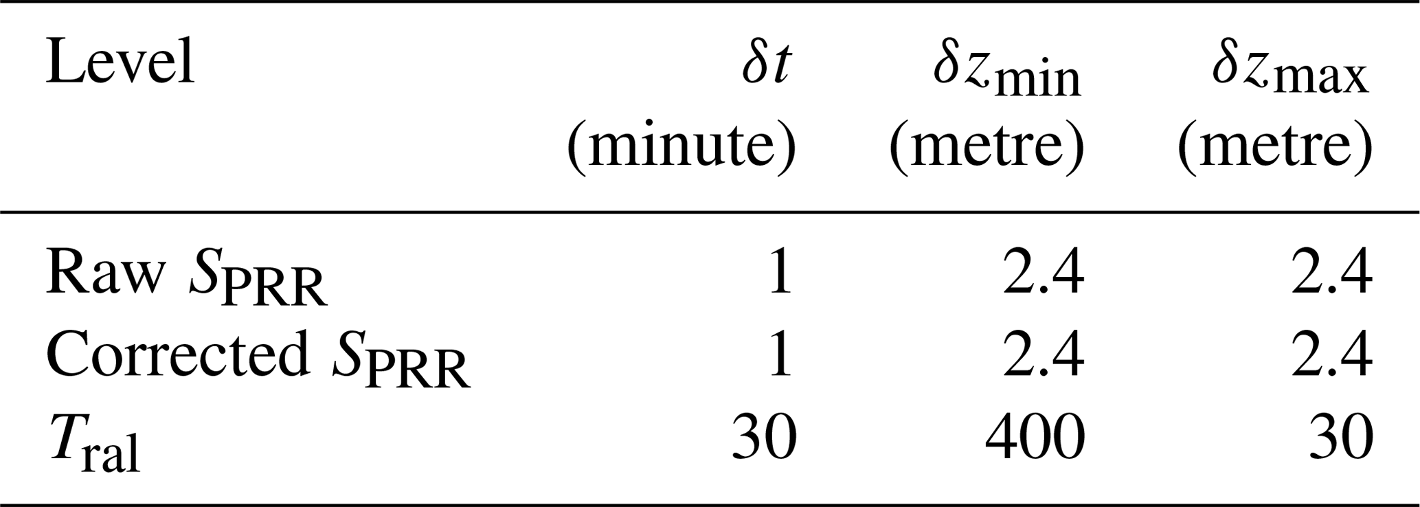
The high- and low-frequency-shifted S_PRR signals have the expression given in Eq. (1). In order to use them to retrieve the temperature profile, Eq. (1) shall be corrected for the dead time and the background. Once the signals are corrected, their ratio is used to retrieve the temperature from Eq. (3) scaled by two coefficients A and B. The atmospheric temperature is then obtained from the calibration of Eq. (3) with respect to T_ors and the determination of A and B. The calibrated temperature is then provided along with its uncertainty. Table 3 summarizes the vertical and temporal resolution of the S_PRR signal at different stages of the data processing. The vertical resolution of T_ral is not constant with altitude and depends on the calculated total random uncertainty in Eq. (6). A Savitzky–Golay digital filter with polynomial degree K=1 is applied to the T_ral profiles to degrade the sampling resolution and reduce the sampling noise. The adopted procedure and the definition of the obtained vertical resolution are compliant with the NDACC (Network for the Detection of Atmospheric Composition Change) recommendations detailed in the work by Leblanc et al. (2016). The initial and highest resolution is δz_max=30 m, which is degraded to a minimum δz_min=400 m corresponding to the regions where the error is large (normally, the upper troposphere and lower stratosphere). For clear-sky measurement, an upper altitude cut-off is set at the altitude where the error exceeds 0.75 K; in the presence of clouds, the upper limit is set by the cloud base detected by a co-located ceilometer. Very often, the clear-sky cut-off altitude corresponds to an altitude between 5 and 7 km during daytime measurements.

Table 3 Spatial and temporal resolution of S_PRR signals and T_ral.

4.1 Correction of S_PRR

The PRR signals are corrected for the systematic underestimation of the true photon-counting signal (dead time) and for the offsets (instrumental and solar). The first correction is then for the acquisition system's dead time τ. The low-transmission channels $J_{\mathrm{high}}^{\mathrm{10}\mathit{\%}}$ and $J_{\mathrm{low}}^{\mathrm{10}\mathit{\%}}$ do not become saturated and are used as reference channels to identify the saturation of the high-transmission channels $J_{\mathrm{high}}^{\mathrm{90}\mathit{\%}}$ and $J_{\mathrm{low}}^{\mathrm{90}\mathit{\%}}$. Assuming that the PMTs and the associated electronics obey the non-paralyzable assumption (Whiteman et al., 1992), we have studied the departure from the constant ratio $J^{\mathrm{10}\mathit{\%}}/J^{\mathrm{90}\mathit{\%}}$ as a function of τ. We have applied a method based on the non-paralyzable condition (Newsom et al., 2009) to a year of data and have calculated τ for all the cases when the saturation clearly affected the high-transmission channels J^90 %.

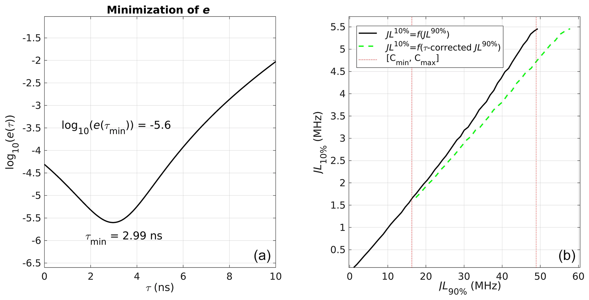
Figure 8 Dead-time calculation and correction of the high-transmission channel J^90 %. Panel (a) shows the minimization of the distance vector e(τ_i) in terms of τ_i yielding the dead time τ=2.99 ns. Panel (b) shows the saturated $J^{\mathrm{10}\mathit{\%}}=f\left(J_{\mathrm{desat}}\right(\mathit{\tau }=\mathrm{0}\left)\right)$ (solid black), the desaturated linear relation J^10 %=f(J_desat(τ_min)) (dashed green) and the count-rate domain [C_min,C_max] (dashed red).

As soon as the saturation has its onset, the ratio $J^{\mathrm{10}\mathit{\%}}/J^{\mathrm{90}\mathit{\%}}$ ceases to be constant and the saturated J^90 % yields smaller count rates than the true ones. When the J^90 % is desaturated using the correct τ, it gives the τ-corrected signal $J_{\mathrm{desat}}\left(\mathit{\tau }\right)=J^{\mathrm{90}\mathit{\%}}/(\mathrm{1}-\mathit{\tau }{J}^{\mathrm{90}\mathit{\%}})$. One-thousand linear fits J^10 %=f(J_desat(τ_i)) are performed with τ_i varying within the interval τ_i∈ [0–10] ns at steps of 0.01 ns. The linear fits J^10 %=f(J_desat(τ_i)) are performed over a temporal interval of 30 min and a vertical range defined by the count rates within the maximum range [0.5–50] MHz: C_min and C_max, respectively. For each linear fit, we calculate the value e(τ_i) that provides the distance in the count-rate domain between J^10 % and f(J_desat(τ_i)) as a function of τ_i. The minimization of e(τ) with respect to τ_i determines the value of the acquisition system's dead time ${\mathit{\tau }}_i={\mathit{\tau }}_{\min }\in$ [0–10] ns for each channel. The obtained value τ_min is used to desaturate J^90 % and to re-establish the constant ratio $J^{\mathrm{10}\mathit{\%}}/f\left(J_{\mathrm{desat}}\right({\mathit{\tau }}_{\min }\left)\right)$, which equals a constant. Figure 8 shows an example calculation of τ_min for the high-transmission channel of J_low. The curve function e(τ) in the figure's left panel has a minimum at τ_min=3 ns. On the right panel, the uncorrected and the τ-corrected relations are shown. The uncorrected relation $J^{\mathrm{10}\mathit{\%}}=f\left(J_{\mathrm{desat}}\right(\mathit{\tau }=\mathrm{0}\left)\right)$ (solid black) departs from the linear relation J^10 %=f(J_desat(τ_min)) (dashed green) as soon as the count rates exceed the lower bound C_min (dashed red). By applying this method to a year of data and collecting more than 100 cases, we have determined the mean dead times τ_jh=1.4 ns and τ_jl=3 ns for J_high and J_low, respectively. The desaturated J_high and J_low are further corrected for the background and the procedure is described hereafter.

The electronic and solar background must be subtracted from S_PRR before retrieving T_ral. While the electronic background is stable and does not undergo daily or seasonal cycles, the solar background changes in intensity with the position of the sun Φ (the angle between the zenith and the centre of the sun's disc). We have found that subtracting the mean value of the far-range signal (z∈ [50–60] km) from S_PRR (subtraction of term B from Eq. 1) causes a systematic negative bias with respect to T_ors of about 1 K at all altitudes z during daytime. A relative change of 1 % in the ratio $J_{\mathrm{low}}/J_{\mathrm{high}}$ due to an imperfect background subtraction can lead to a variation of up to 2 K in the retrieved temperature T_ral. Because the solar background (SB) dominates the total background of S_PRR, we focus on the correction of the background B only as a function of the position of the sun. We have developed an empirical correction function f(Φ) applied to the background prior to subtraction from S_PRR. The function f(Φ) is applied to the background B and provides the corrected background $B_{\mathrm{corr}}=f\left(\mathrm{\Phi }\right)\cdot B$. Through the year's cycle, B is reduced by a maximum amount of 1 % via the action of f(Φ). As Eq. (2) shows, f(Φ) reaches daily minima when $\mathrm{\Phi }={\mathrm{\Phi }}_{\min }^{\mathrm{day}}$ (noon) and returns to 100 % when Φ≥90^∘ (after sunset and before sunrise). During the daily and annual cycle, f(Φ) then oscillates within the range f(Φ)∈ [99 %–100 %], reducing B by the maximum amount of 1 % (f(Φ)=99 %) at noon on 21 June when $\mathrm{\Phi }={\mathrm{\Phi }}_{\min }^{\mathrm{year}}$.

$$\begin{array}{}\text{(2)}& {\displaystyle }\begin{array}{rl}& f\left(\mathrm{\Phi }\right)=\mathrm{1}-\mathrm{0.01}\cdot {\displaystyle \frac{\cos \mathrm{\Phi }}{\cos {\mathrm{\Phi }}_{\min }}}{\mathit{\delta }}_{\mathrm{\Phi }};{\mathit{\delta }}_{\mathrm{\Phi }}\equiv \mathrm{1}\text{for}\mathrm{0}\le \mathrm{\Phi }<\mathit{\pi }/\mathrm{2},\\ & {\mathit{\delta }}_{\mathrm{\Phi }}\equiv \mathrm{0}\text{for}\mathit{\pi }/\mathrm{2}\le \mathrm{\Phi }<\mathrm{2}\mathit{\pi }.\end{array}\end{array}$$

If uncorrected, the retrieved daytime T_ral suffers a bias at all heights with respect to T_ors. The bias is largest when $\mathrm{\Phi }={\mathrm{\Phi }}_{\min }^{\mathrm{day}}$. The correction f(Φ) is applied only to the background of J_high. The intensity of J_high is generally lower than J_low at all atmospheric temperatures (see Sect. 4) and so is its signal-to-noise ratio (SNR). Even a small error of ≈1 % when subtracting B from J_high has a major impact on its SNR; f(Φ) corrects the imperfect subtraction of B from J_high and minimizes the daytime bias of T_ral with respect to T_ors almost perfectly.

4.2 Estimation of total random uncertainty

Once B_corr is subtracted from the τ-corrected S_PRR, the deviation of T_ral from T_ors depends only on how precisely Eq. (3), derived from the RLE, represents the true atmospheric temperature at the altitude z and time t. The random uncertainty does not account for the error induced by the saturation and the background, which are considered purely systematic. The high-frequency-shifted (J_high) and low-frequency-shifted (J_low) signals in the Stokes and anti-stokes Q branches depend on the temperature of the probed atmospheric volume (Fig. 4). The ratio of the S_PRR intensities $Q\left(z\right)=J_{\mathrm{low}}\left(z\right)/J_{\mathrm{high}}\left(z\right)$ is a function of the atmospheric temperature T at the distance z. Based on the calculations shown by Behrendt (2005) and for systems that can detect independent J lines in each channel, the relationship between T and Q would take the form of Eq. (3) with an equals (=) sign. The approximately equal to sign (≈) in Eq. (3) indicates that the detection system detects more than one J line and thus brings an inherent error. The calibration coefficients A and B are a priori undetermined and can be determined by calibration of T_ral with respect to T_ors.

$$\begin{array}{}\text{(3)}& T_{\mathrm{ral}}\approx {\displaystyle \frac{A}{B+\ln Q}}.\end{array}$$

The coefficients A and B are determined by calibrating T_ral with respect to T_ors. The coefficient A has units in kelvin as Eq. (3) is not normalized for the standard atmospheric temperature (Behrendt and Reichardt, 2000). The linear relation $y=A/(x+B)$ is used, where x is the ratio Q, and y is the reference temperature T_ors. The mean error on T_ors for both RS41 and SRS-C50 is $\approx -\mathrm{0.04}\pm \mathrm{0.15}$ K at 11:00 and 23:00 UTC between 0 and 14 km (Sect. 2). Due to the very small error on T_ors, we can calculate the uncertainty U_fit of the fitting model only in terms of the fitting parameters' errors σ_A and σ_B (Eq. 4). As it will be shown in the next section, the covariance σ_AB of A and B is very close to zero ($<{\mathrm{10}}^{-\mathrm{3}}$); thus, σ_A and σ_B can be treated as statistically independent and used to calculate U_fit from the first-order Taylor series of propagation of fitting parameter uncertainties.

$$\begin{array}{}\text{(4)}& U_{\mathrm{fit}}={\displaystyle \frac{\mathrm{1}}{(B+\ln Q)}}{\left[{\mathit{\sigma }}_A^{\mathrm{2}}+{\displaystyle \frac{A^{\mathrm{2}}{\mathit{\sigma }}_B^{\mathrm{2}}}{{\left(B+\ln Q\right)}^{\mathrm{2}}}}\right]}^{\frac{\mathrm{1}}{\mathrm{2}}}.\end{array}$$

U_fit is not the only error source; a second contribution to the total uncertainty comes from the fact that S_PRR is acquired by a photon-counting system and is affected by the measurement's noise that can be calculated using standard Poisson statistics. The error σ_J for Poisson-distributed data is equal to the square root of the S_PRR signals, ${\mathit{\sigma }}_{J_{\mathrm{low}}}=\sqrt{J_{\mathrm{low}}}$ and ${\mathit{\sigma }}_{J_{\mathrm{high}}}=\sqrt{J_{\mathrm{high}}}$. In Eq. (5), coefficients A and B can be regarded as independent from the noise on S_PRR, as the contribution of it is already included in σ_A and σ_B in Eq. (4).

$$\begin{array}{}\text{(5)}& U_{\mathrm{sig}}={\displaystyle \frac{A}{(B+\ln Q{)}^{\mathrm{2}}}}{\left[{\displaystyle \frac{\mathrm{1}}{J_{\mathrm{high}}}}+{\displaystyle \frac{\mathrm{1}}{J_{\mathrm{low}}}}\right]}^{\frac{\mathrm{1}}{\mathrm{2}}}.\end{array}$$

The total uncertainty of the calibrated T_ral is a type-B uncertainty (JCGM, 2008) and is the sum of the independent error contributions U_fit and U_sig.

$$\begin{array}{}\text{(6)}& \begin{array}{rl}{U}_T& =\sqrt{U_{\mathrm{fit}}^{\mathrm{2}}+U_{\mathrm{sig}}^{\mathrm{2}}}\\ & =\sqrt{{\displaystyle \frac{\mathrm{1}}{{\left(B+\ln Q\right)}^{\mathrm{2}}}}\left[{\mathit{\sigma }}_A^{\mathrm{2}}{\left(B+\ln Q\right)}^{\mathrm{2}}+A^{\mathrm{2}}\left({\mathit{\sigma }}_B^{\mathrm{2}}+{\displaystyle \frac{\mathrm{1}}{J_{\mathrm{high}}}}+{\displaystyle \frac{\mathrm{1}}{J_{\mathrm{low}}}}\right)\right]}.\end{array}\end{array}$$

4.3 Calibration of S_PRR

For a very stable system like RALMO, calibrations can be performed once every few months to compensate for any occurring drift of the detection system's sensitivity and/or efficiency. Calibrations of RALMO are performed using Eq. (3) in clear-sky conditions during nighttime to remove the effect of solar background and have a larger vertical portion of T_ral available for calibration (the daytime profiles have normally a lower cut-off altitude). Figure 9 shows a case of RALMO calibration; the green-shaded area represents ±2U_T (k=2).

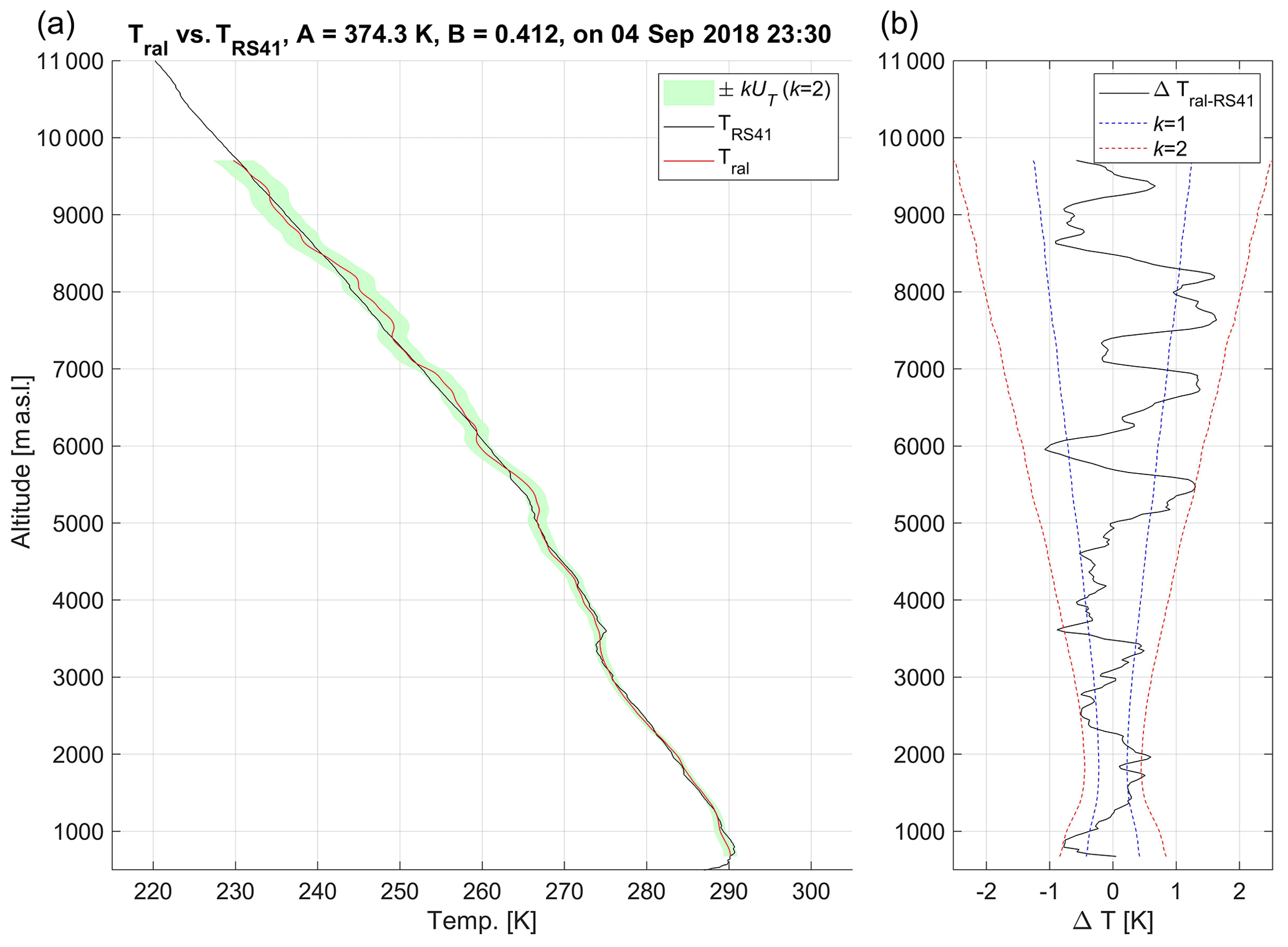
Figure 9 RALMO temperature profile calibrated by the ORS RS41. Panel (a) shows T_RS41 (solid black) and T_ral (solid red) with the confidence interval (green shading) corresponding to kU_T(k=2). Panel (b) shows the differences ΔT_ral−RS41 within the U_T k-boundaries for k=1 (dashed blue) and k=2 (dashed red).

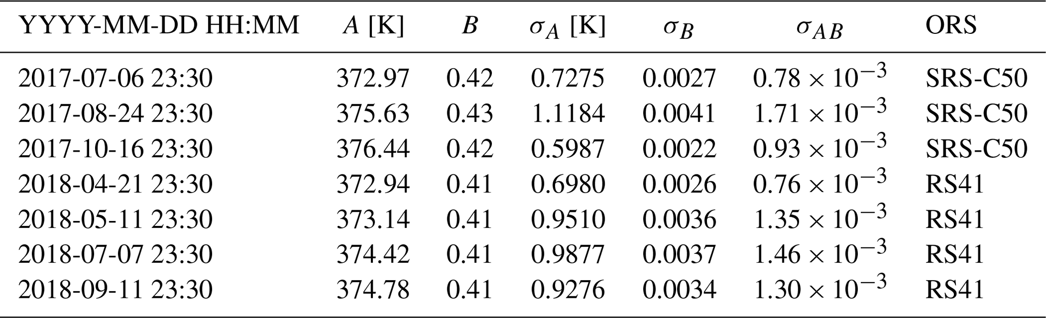
The calibrated T_ral results from the integration of 30 τ- and B-corrected S_PRR profiles (δt=30 min) into Eq. (3). At a given atmospheric altitude z during the time interval δt, U_T(z)|_δt is made of the single contributions U_sig(z,t) and U_fit(z,t). U_sig(z,t) can be regarded as independent with respect to time; on the other hand, the errors U_fit(z,t) depend on the atmospheric processes occurring within the layer [$z-\mathit{\delta }z/\mathrm{2},z+\mathit{\delta }z/\mathrm{2}$] during the time interval [$t-\mathit{\delta }t/\mathrm{2},t+\mathit{\delta }t/\mathrm{2}$] and are, a priori, not statistically independent. By assuming that all errors in Eq. (6) are statistically independent, we assume that the off-diagonal elements of the variance–covariance matrix are all zero. By doing so, U_T(z)|_δt could be underestimated by an amount equal to the non-zero covariance terms, including the covariance σ_AB. A method to assess the exhaustiveness of the theoretical error U_T is to calculate how many points in the vector $\mathrm{\Delta }T=T_{\mathrm{ral}}-T_{\mathrm{ors}}$ fall within the interval $[-k\mathit{\sigma },+k\mathit{\sigma }]$ and check if they are compatible with the Gaussian probability levels 68.3 %, 95.5 % and 99.7 % for $k=\mathrm{1},\mathrm{2}$, and 3, respectively. As it is shown in the right panel of Fig. 9, almost all points along the vector T_ral−T_ors fall within the interval $[-\mathrm{2}\mathit{\sigma },+\mathrm{2}\mathit{\sigma }]$, i.e. the 98.1 % envelope. For k=1, the percentage falls slightly below the expected level for a normal distribution with only 61.2 % of the points within $[-\mathit{\sigma },+\mathit{\sigma }]$. Between July 2017 and December 2018, a total of seven calibrations have been performed (three SRS-C50 and four Vaisala RS41). The mean percentage of points over all performed calibrations is 65.1 % for k=1; 97.9.1 % for k=2; and 99.98 % for k=3. These values seem to confirm an overall exhaustiveness of U_T with a slight underestimation of 3.2 % at k=1. The list of calibrations is shown in Table 4. For each calibration, the table lists the date and end time of the calibration, the calibration coefficients A and B used in the fitting model Eq. (3), the errors σ_A and σ_B, the covariance σ_AB, and the ORS used to calibrate T_ral. As to further support the assumption of zero covariance of the coefficients A and B, all covariances σ_AB in the table are smaller than $\mathrm{1.71}\times {\mathrm{10}}^{-\mathrm{3}}$. Between two consecutive calibrations performed at times t_i and t_i+1, the coefficients A(t_i) and B(t_i) are used to calibrate all profiles T_ral during the time interval $t\in [t_i,t_{i+\mathrm{1}}]$.

Table 4 Calibrations of RALMO T profiles by the working standard.

5 Validation of PRR temperature

More than 450 profiles T_ral (245 nighttime, 215 daytime) have been compared to T_ors and assessed separately for daytime and nighttime based on the bias and standard deviation (σ) of the differences $\mathrm{\Delta }T=T_{\mathrm{ral}}-T_{\mathrm{ors}}$ over the period 1 July 2017–31 December 2018. Two criteria to select the cases for the dataset have been used:

• 1.

  Only cases with no precipitation and no low clouds or fog are retained.

• 2.

  Only cases with ΔT<5 K are retained.

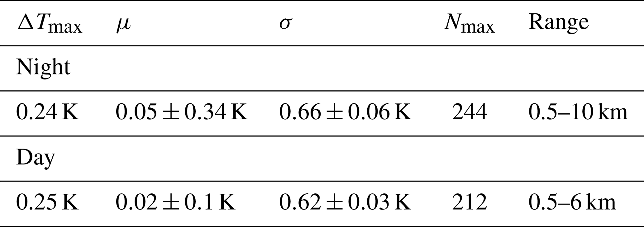
Criterion 1 is performed by setting a threshold for minimum cloud base, h_b, at 1000 m (a.g.l.), for any values of h_b<1000 m that T_ral is not retrieved. Whenever h_b>1000 m, the cut-off altitude will correspond to h_b. Indeed, above h_b, the SNR drops abruptly and U_T(z)≫1 K. For this reason, especially during winter, when long-lasting stratus clouds occur in the altitude range 1–4 km, the nighttime and daytime T_ral profiles are limited in range to the altitude h_b (or are not calculated if h_b<1000 m). Criterion 2 is performed by setting a threshold at 33 % of the number of elements along the profile ΔT exceeding 5 K. If more than 33 % of the elements along ΔT exceed the threshold, the whole of T_ral is rejected and not included in the statistics. For any value below the threshold, the outliers are removed from T_ral. This is justified by the fact that exceedances counting more than 33 % are caused by temporary misalignment of the transceiver unit. On the other hand, exceedances well below the threshold can always occur (especially in the higher part of the profile) due to low SNR or unfiltered clouds. In Table 5 we present a summary of the statistical parameters characterizing the daytime and nighttime differences ΔT that will be discussed in detail in the following sections. The dataset ΔT is described in terms of maximum mean bias ΔT_max, average mean bias μ, standard deviation σ and maximum availability N_max of the differences ΔT along the atmospheric range.

Table 5 Summary of the statistical parameters of the day and night ΔT dataset.

Besides a global validation, we also present and discuss the seasonal statistics in order to better characterize the system performance.

5.1 Nighttime temperature statistics

The nighttime ΔT_max, μ, σ and N_max of ΔT are the metrics to assess the accuracy and precision of T_ral with respect to T_ors. Figure 10 shows that ΔT_max=0.24 K, $\mathit{\mu }=\mathrm{0.05}\pm \mathrm{0.34}$ K, $\mathit{\sigma }=\mathrm{0.66}\pm \mathrm{0.06}$ K and N_max=244 over the tropospheric region [0.5–10] km.

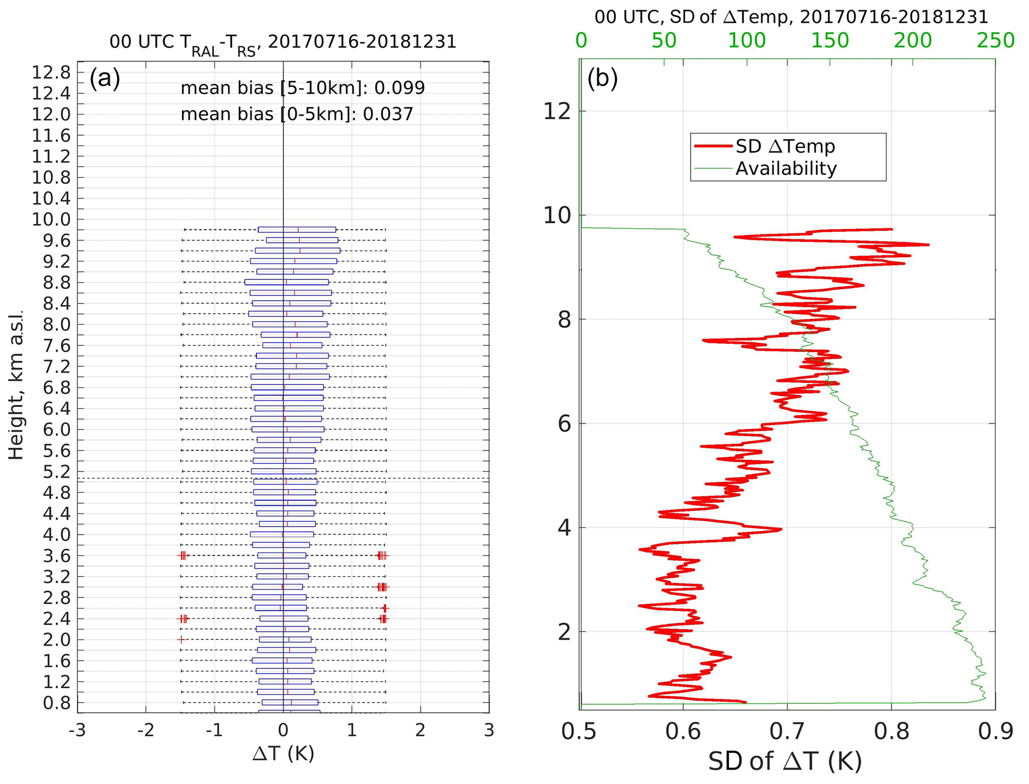
Figure 10 Nighttime bias and standard deviation (SD) of ΔT over the period July 2017–December 2018. In (a), on each box of 200 m vertical span, the central mark indicates the median, and the left and right edges of the box indicate the 25th and 75th percentiles, respectively. The whiskers extend to the most extreme data points not considered outliers, and the outliers are plotted individually and shown by the “+” symbol. The thick red curve in the right panel shows the vertical profile of SD calculated over the altitude-decreasing number of ΔT points (thin green).

In addition to the uncertainty assessment performed in Sect. 4.3, the exhaustiveness of the theoretical total uncertainty U_T can be further assessed by comparing U_T with σ. The mean value of U_T along the troposphere and over the seven nighttime calibrations is ${\stackrel{\mathrm{‾}}{U}}_T=\mathrm{0.64}$ K; the mean nighttime standard deviation averaged over the tropospheric column in Fig. 10 is $\stackrel{\mathrm{‾}}{\mathit{\sigma }}=\mathrm{0.66}$ K. The two 1−k uncertainties are then fully compatible.

The nighttime ΔT data are characterized by values of μ and σ smaller than 1 K, with minimum values in the lower troposphere from [0–5] km. It is indeed in the lower troposphere, where σ is ≈0.6 K, i.e. 0.1 K larger than the 0.5 K requirement for data assimilation into the numerical weather prediction COSMO forecasting system (Fuhrer et al., 2018; Klasa et al., 2018, 2019). In order to achieve a successful assimilation of T_ral into COSMO, the overall impact of the assimilation shall correspond to an improvement of the forecasts without increasing the forecast uncertainties. Assimilation of high-SNR, well-calibrated T_ral into numerical models leads to the improvement of the forecasts. In the study by Leuenberger et al. (2020), the authors assimilate, amongst other data, temperature and humidity profiles from RALMO, showing the beneficial impact on the precipitation forecast over a wide geographical area.

5.2 Daytime temperature statistics

During daytime, the retrieved temperature profiles are limited in range to about 6 km. The left and right panels of Fig. 11 show the bias ΔT and the standard deviation σ, respectively. The ΔT_max, μ, σ and N_max of the daytime ΔT over the lower troposphere (0.5–6 km) are 0.25 K, 0.02±0.1 K, 0.62±0.03 K and 212, respectively. The data availability goes rapidly to zero above 5 km.

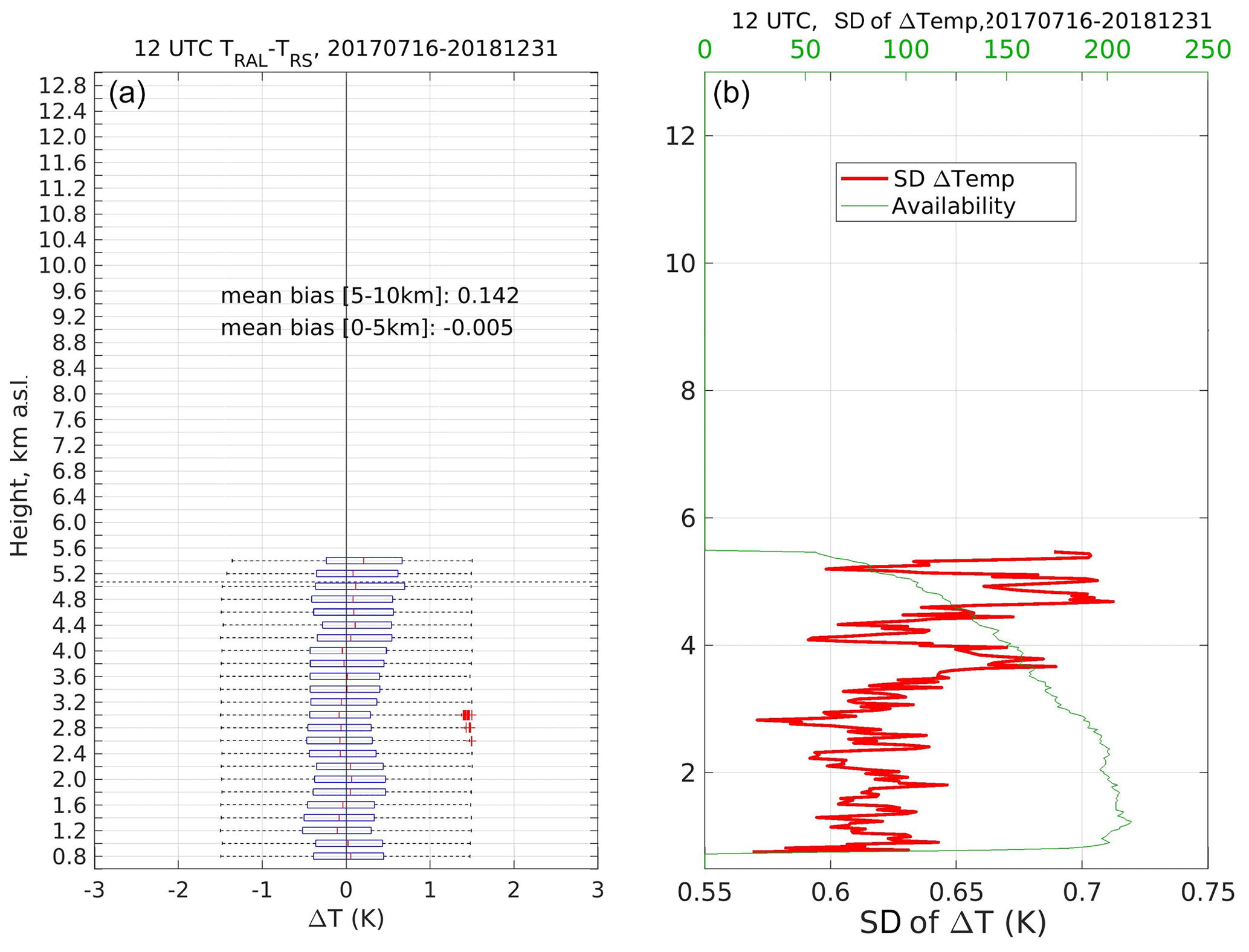
Figure 11 Daytime bias and standard deviation (SD) of ΔT over the period July 2017–December 2018. In (a), on each box of 200 m vertical span, the central mark indicates the median, and the left and right edges of the box indicate the 25th and 75th percentiles, respectively. The whiskers extend to the most extreme data points not considered outliers, and the outliers are plotted individually and shown by the “+” symbol. Panel (b) shows the vertical profile of standard deviation (thick red) calculated over the altitude-decreasing number of ΔT points (thin green).

The daytime T_ral profiles have been corrected for the solar background by f(Φ), which proves to be very efficient in removing the noon bias with respect to T_ors. To ensure that the correction f(Φ) does not introduce any additional bias during the daily cycle, we have compared T_ral with the temperature calculated by the COSMO model. More than 3 months of clear-sky 24 h T_ral−T_cos differences have been collected, yielding a mean daily cycle at the level 1.4–1.7 km a.s.l. The comparison in Fig. 12 shows that RALMO does not suffer any systematic daily Φ-dependent bias.

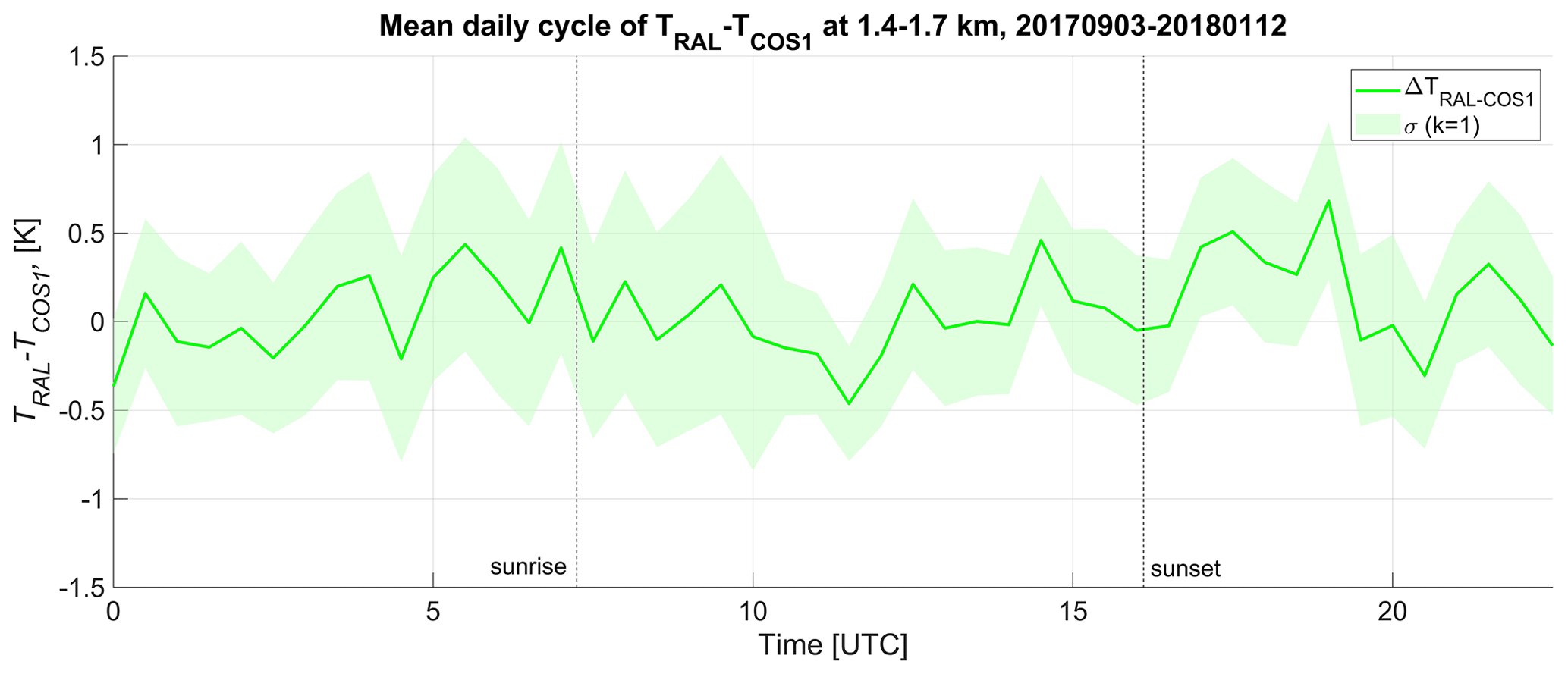
Figure 12 Differences between RALMO and COSMO temperature at 1400–1700 m a.s.l. during September 2017–January 2018. The green shading accounts for the k=1 standard deviation of the differences. The dashed vertical lines show the sunrise and sunset time on 12 January 2018; the mean daily cycle shows that no artefacts are introduced by the application of f(Φ) during daylight.

6 Seasonality study

In order to study the seasonal effects on μ and σ, the ΔT dataset was divided into seasons. The four seasons are defined as follows: summer from 1 June to 30 August, autumn from 1 September to 30 November, winter from 1 December to 15 March, and spring from 16 March to 31 May. Because of the less favourable conditions in winter due to precipitation and low clouds, only few temperature profiles are available during this period. Additionally, during winter 2018, from January until mid-March, RALMO measurements have been stopped for about 80 % of the time due to maintenance work. The results are summarized in Tables 6 and 7 in terms of μ, σ and maximum availability N_max over the lower tropospheric range 0–6 km for daytime and over 0–10 km for nighttime. With the only exception of winter, the other seasons have enough profiles to perform a statistical analysis and to draw quantitative conclusions about the contribution of each season to the overall values μ and σ.

6.1 Seasonal daytime temperature statistics

The seasonal daytime μ and σ profiles are analysed to understand if sources of systematic errors other than SB affect the retrieved T_ral. The seasonal profiles are shown in Figs. 13 and 14 and summarized in Table 6. Due to the less favourable weather conditions and the maintenance work, the winter statistics count only eight profiles. The statistical characterization of the winter dataset can then only be qualitative. Summer and spring are the seasons with the minimum values of Φ at noon; during these two seasons, T_ral is most affected by SB. If uncorrected for f(Φ), the noon T_ral suffers a negative mean bias of about 2 K at all heights (not shown here). Summer counts more than twice the number of cases in the spring dataset; nevertheless, for both seasons the values of μ are compatible with a zero bias within their uncertainties (both σ=0.64 K). Despite the less favourable weather conditions compared to spring and summer, autumn is the season with most cases, and this is because there are two autumn seasons in the dataset. Like spring and summer, autumn also has μ compatible with the zero bias within its uncertainty. Through the four seasons, the mean σ spans from 0.4 to 0.65 K.

Table 6 Seasonal mean bias μ, standard deviation σ and maximum availability N_max at 12:00 UTC.

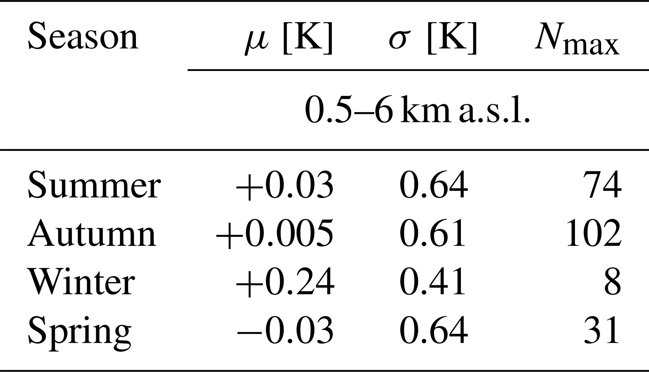
Figure 13 suggests that T_ral is not affected by any obvious systematic error ($\mathit{\mu }\simeq \mathrm{0}\in [-\mathit{\sigma },+\mathit{\sigma }]$) and no seasonal cycle appears in the statistics. From the perspective of the statistical validity of the studied data, any subsample chosen randomly from the total T_ral dataset can be described by the same μ and σ that characterizes ΔT.

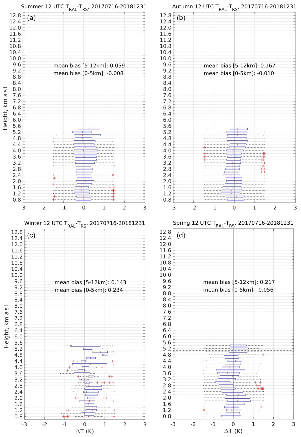
Figure 13 Seasonal daytime bias of ΔT over the period July 2017–December 2018. The boxplot characteristics are the same as in Figs. 10 and 11 but restricted over the seasonal periods. Based on the definition of seasons provided in the text, in clockwise order starting form the upper-left corner, panel (a) shows the summer data, panel (b) shows the autumn data, panel (c) shows the winter data and panel (d) shows the spring data.

Unlike Fig. 13, the σ profiles in Fig. 14 show different behaviours in summer–autumn and in winter–spring. The summer and autumn σ profiles in the upper-left and upper-right panels undergo a decoupling between the lower and upper part of the profile with inversion point slightly higher in autumn. An increase in σ with height is something expected and can be explained with the decreased data availability and the decreased SNR due to the large distance from the lidar's telescope. However, the abrupt increase in σ at ≈3 km in summer and at ≈4.5 km in autumn is more related to the atmospheric dynamics than to the SNR. In summer, the transition between the boundary layer and the free troposphere is a region of high variability in terms of temperature and humidity. The alternating cold downdraughts and warm updraughts engendered by the overall fair weather conditions and the continuous development of thermals through the boundary layer (Martucci et al., 2010) cause a large variability of T_ral at ≈3 km, which translates into large σ values. In autumn, the thermal activity at the top of the boundary layer is less pronounced than in summer; on the other hand, a temperature inversion linked to the formation and dissipation of stratus clouds above Payerne occurs at ≈4.5 km, causing larger discrepancies in the comparison with T_ors.

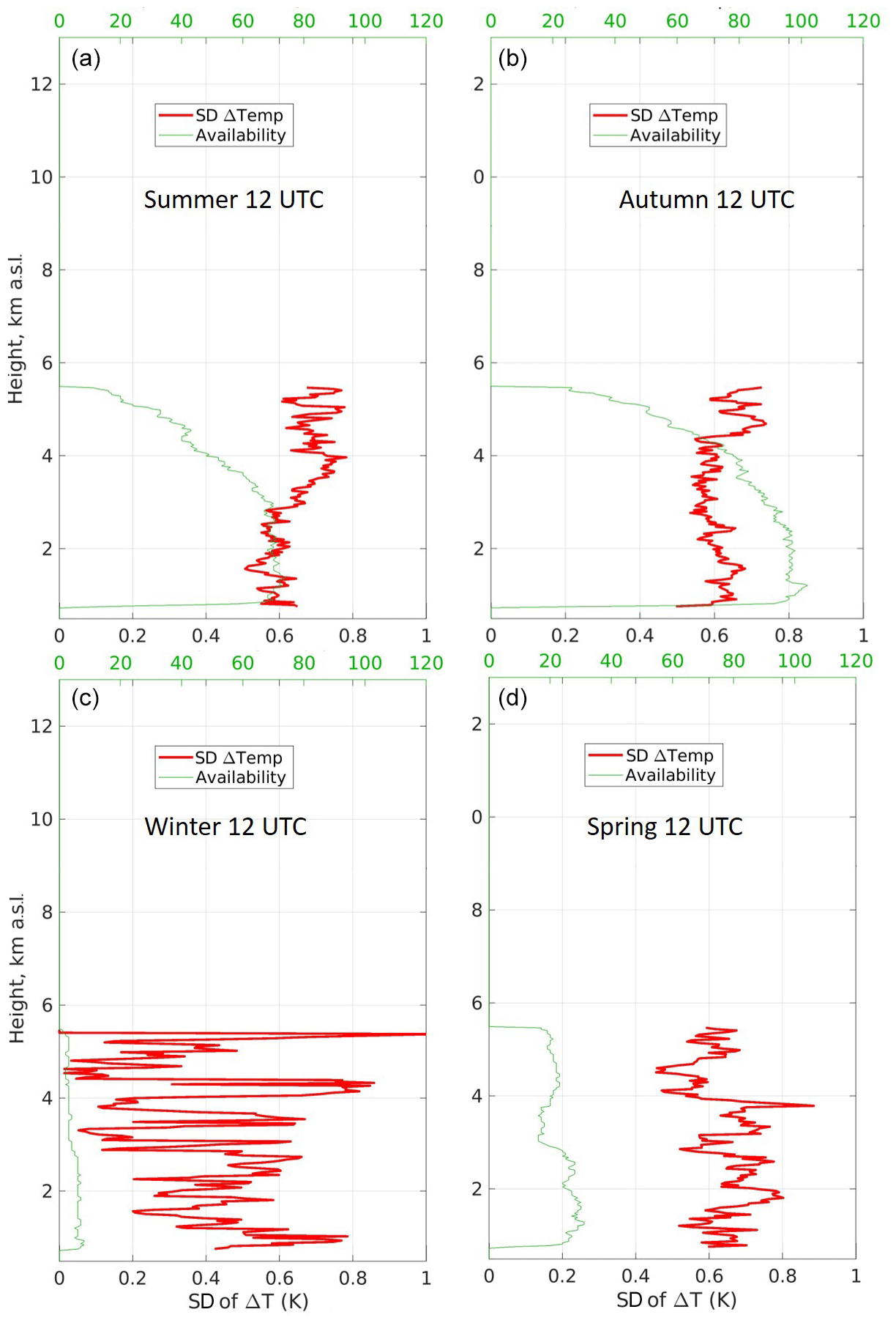
Figure 14 Seasonal daytime standard deviation (SD) of ΔT over the period July 2017–December 2018. The vertical profiles of standard deviation (thick red) are calculated over the altitude-decreasing number of ΔT points (thin green). Based on the definition of seasons provided in the text, in clockwise order starting form the upper-left corner, panel (a) shows the summer data, panel (b) shows the autumn data, panel (c) shows the winter data and panel (d) shows the spring data.

6.2 Seasonal nighttime temperature statistics

At nighttime, f(Φ) has no impact on the temperature retrieval, and the seasonal statistics can reveal sources of systematic error other than the SB causing $\left|\mathit{\mu }\right|>\mathrm{0}$. The separation into seasons helps with understanding if the overall zero bias shown in Fig. 10 hides seasonal non-zero biases that cancel out when combined in the full dataset. Compared to the daytime cases (215), the availability of the nighttime dataset is higher (245), including the winter dataset, which allows us to perform a statistical analysis for all seasons.

Table 7 Seasonal mean bias μ, standard deviation σ and maximum availability N_max at 00:00 UTC.

All seasonal μ values are compatible with the zero bias along the troposphere within $[-\mathit{\sigma },+\mathit{\sigma }]$. Like the daytime seasonal statistics, the nighttime also does not reveal any obvious source of systematic error. The mean μ and σ in the troposphere are summarized in Table 7.

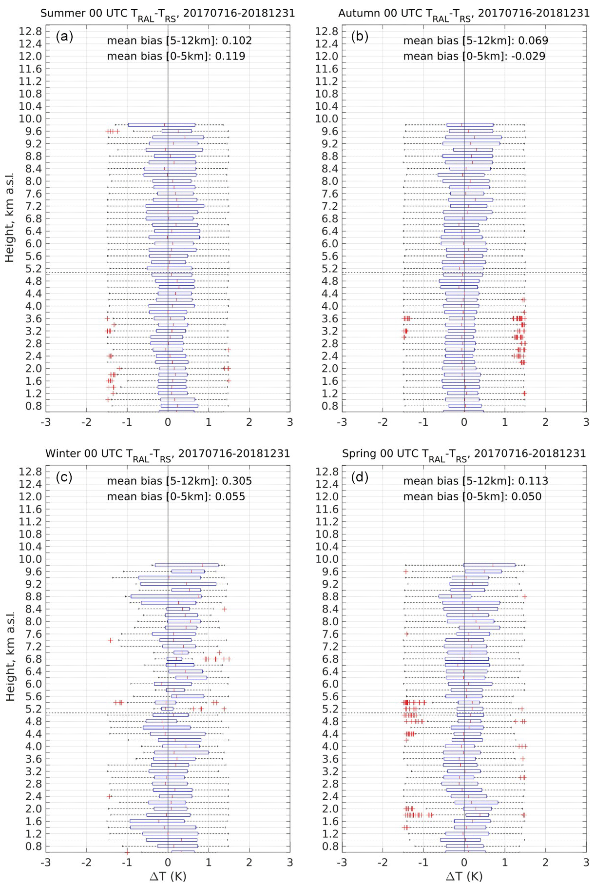
Figure 15 Seasonal nighttime bias of ΔT over the period July 2017–December 2018. The boxplot characteristics are the same as for Figs. 10 and 11 but restricted over the seasonal periods. Based on the definition of seasons provided in the text, in clockwise order starting form the upper-left corner, panel (a) shows the summer data, panel (b) shows the autumn data, panel (c) shows the winter data and panel (d) shows the spring data.

The nighttime atmosphere undergos different dynamics with respect to daytime. The absence of solar radiation almost entirely removes the convection from the boundary layer and minimizes the variance of the temperature at the top of the nocturnal and residual layers. Consequently, no sharp increase in the σ values is detected at any specific level during the different seasons. The σ profiles increase their value with height in response to the drop of the SNR due to the distance from the emission.

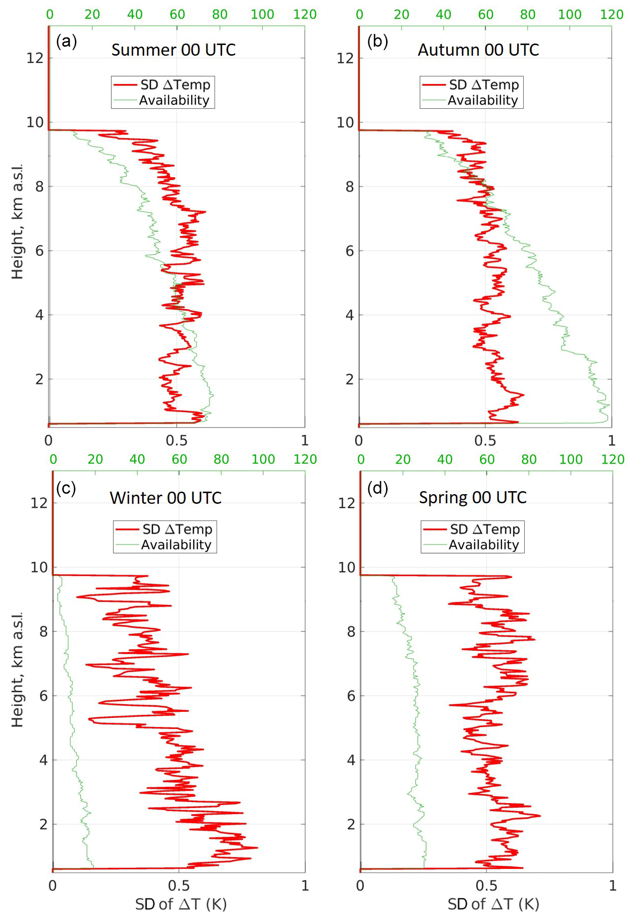
Figure 16 Seasonal nighttime standard deviation (SD) of ΔT over the period July 2017–December 2018. The vertical profiles of standard deviation (thick red) are calculated over the altitude-decreasing number of ΔT points (thin green). Based on the definition of seasons provided in the text, in clockwise order starting form the upper-left corner, panel (a) shows the summer data, panel (b) shows the autumn data, panel (c) shows the winter data and panel (d) shows the spring data.

7 Future applications

The validated T_ral is used to calculate the relative humidity using the humidity profiles also provided by RALMO. The relative humidity product has been validated in a parallel work by Navas-Guzmán et al. (2019) that shows that in the first 2 km the RH suffers a mean systematic and random error of $\mathrm{\Delta }\text{RH}=+\mathrm{2}\mathit{\%}\pm \mathrm{6}\mathit{\%}\text{RH}$. The validated RH can be used to perform, amongst others, studies of supersaturation of water vapour in liquid stratus clouds. As future work, we will investigate the supersaturation corrected for the RH systematic error in a large statistical dataset of liquid clouds above Payerne across different seasons and years. The possibility to study supersaturation is critical to disentangle the microphysics of liquid clouds and better predict the amount of liquid water within the cloud.

8 Conclusions

More than 450 lidar temperature profiles have been compared to the temperature profiles measured by the reference radiosounding system at Payerne at 11:00 and 23:00 UTC during 1.5 years (July 2017–December 2018). The reference radiosounding systems (SRS-C50 and Vaisala RS41) have been validated by the GRUAN-certified Vaisala RS92 sonde in the framework of the quality assurance programme carried out at Payerne. A semi-empirical modification has been developed and applied to the background correction procedure to reduce the daytime bias. The temperature profiles retrieved from RALMO PRR data show an excellent agreement with the reference radiosounding system during both daytime and nighttime in terms of maximum bias (ΔT_max), mean bias (μ) and standard deviation (σ). The ΔT_max, μ and σ of the daytime differences $\mathrm{\Delta }T=T_{\mathrm{ral}}-T_{\mathrm{ors}}$ over the tropospheric region (0.5–6 km) are 0.28, 0.02±0.1 and 0.62±0.03 K, respectively. The nighttime ΔT dataset is characterized by a mean bias $\mathit{\mu }=\mathrm{0.05}\pm \mathrm{0.34}$ K and $\mathit{\sigma }=\mathrm{0.66}\pm \mathrm{0.06}$ K, while ΔT is smaller than ΔT_max=0.29 K at all heights over the tropospheric region (0.5–10 km). We have compared the lidar temperature data against the temperature predicted by the COSMO model and found that there was no dependence of the bias and the standard deviation on the diurnal cycle. This result let us conclude that essentially the same data quality is achieved at day and night. A seasonality study has been performed to help with understanding if the obtained overall daytime and nighttime zero bias hides seasonal non-zero biases that cancel out when combined in the full dataset. The study reveals that all independent seasonal contributions of μ are compatible with the zero bias within their uncertainty. In general, the seasonal datasets confirm the fact that when subsampling the total ΔT dataset the subsamples can still be described by the same μ and σ.

We have shown that the temperature profiles obtained from the PRR RALMO data meet the OSCAR breakthrough uncertainty requirement of 1 K for high-resolution NWP (https://www.wmo-sat.info/oscar/requirements, last access: 1 February 2021). Combined with the water vapour measurements the Raman lidar has a high potential to improve NWP through data assimilation as we have demonstrated recently (Leuenberger et al., 2020), and MeteoSwiss plans to assimilate the Raman lidar in Payerne operationally in the near future.