the Creative Commons Attribution 4.0 License.
the Creative Commons Attribution 4.0 License.
 | 25 Feb 2021
Estimation of the height of the turbulent mixing layer from data of Doppler lidar measurements using conical scanning by a probe beam
Viktor A. Banakh
Igor N. Smalikho
Andrey V. Falits
A method is proposed for determining the height of the turbulent mixing layer on the basis of the vertical profiles of the dissipation rate of turbulent energy, which is estimated from lidar measurements of the radial wind velocity using conical scanning by a probe beam around the vertical axis. The accuracy of the proposed method is discussed in detail. It is shown that for the estimation of the mixing layer height (MLH) with the acceptable relative error not exceeding 20 %, the signal-to-noise ratio should be no less than −16 dB, when the relative error of lidar estimation of the dissipation rate does not exceed 30 %. The method was tested in a 6 d experiment in which the wind velocity turbulence was estimated in smog conditions due to forest fires in Siberia in summer 2019. The results of the experiment reveal that the relative error of determination of the MLH time series obtained by this method does not exceed 10 % in the period of turbulence development. The estimates of the turbulent mixing layer height by the proposed method are in a qualitative agreement with the MLH estimated from the distributions of the Richardson number in height and time obtained during the comparison experiment in spring 2020.
- Article
(2806 KB) - Full-text XML
- BibTeX
- EndNote


The turbulent mixing layer in the lower part of the Earth's atmosphere has an important role in the vertical transport of moisture, small gas constituents, pollutants, and heat from the surface to the upper layers of the atmosphere. The turbulent mixing layer height is usually understood to be the thickness of the layer adjacent to the ground, in which incoming substances become completely vertically distributed throughout the layer owing to convection or turbulence for an hour (Stull, 1988; Garratt, 1994; Bonin et al., 2018). Among other factors (Garratt, 1994), the mixing layer height strongly depends on the intensity of wind turbulence.
There are different technical facilities that are widely used for turbulent parameter estimation in the atmospheric boundary layer (ABL) and determining the mixing layer height. Doppler sodars, radio acoustic systems, and Doppler lidars are the most suitable for this task, as they allow for meteorological data to be measured in real time with the required space and time resolution (Bonin et al., 2018; Emeis et al., 2008; Hogan et al., 2009; Tucker et al., 2009; Pichugina and Banta, 2010; Barlow et al., 2011; Helmis et al., 2012; Schween et al., 2014; Vakkari et al., 2015; Huang et al., 2017; Petenko et al., 2019). From the data of lidar measurements, the variance of radial velocity , variances of vertical and horizontal and wind vector components, turbulence kinetic energy (TKE) E(h), and turbulent energy dissipation rate ε(h) can be estimated at different heights h.
In Bonin et al. (2018), Hogan et al. (2009), Tucker et al. (2009), Pichugina and Banta (2010), Barlow et al. (2011), Schween et al. (2014), Vakkari et al. (2015), and Huang et al. (2017), the mixing layer height (MLH) hmix was determined from the decrease in the variance ( are indexes for designating the radial, vertical, and two horizontal components of wind velocity vector, respectively) with height h down to some minimum threshold value , at which the turbulence intensity becomes insufficient for efficient air mixing. The variances and MLH were estimated from pulsed coherent Doppler lidar (PCDL) data through the use of various measurement strategies and data processing algorithms (Bonin et al., 2018; Hogan et al., 2009; Tucker et al., 2009; Pichugina and Banta, 2010; Barlow et al., 2011; Schween et al., 2014; Vakkari et al., 2015; Huang et al., 2017; Manninen et al., 2018): (i) in the fixed strictly vertical direction of the probing beam (vertical stare mode), (ii) by scanning in vertical plane, and (iii) by conical scanning by a beam around the vertical axis at a certain elevation angle φ. In Bonin et al. (2018), the “composite fuzzy logic approach” based on the use of all three measurement geometries was applied to determine hmix.
According to analysis (Tucker et al., 2009), lidar measurements of the vertical profile of the variance of vertical velocity in the fixed vertical probing direction provide the best accuracy of estimation of the mixing layer height hmix. However, it was shown (Bonin et al., 2018) that this is not always the case. In particular, during the propagation of internal gravity waves (IGWs), this method may significantly overestimate hmix, and it becomes necessary to perform high-frequency filtering of the data.
The turbulence energy dissipation rate, as well as variances of the fluctuations of wind vector components, characterizes the turbulence (air mixing) intensity and can also be used for the estimation of hmix. This was done for the first time in Vakkari et al. (2015), in which the diurnal profile of hmix(t), where t is time, was determined from the space–time distributions of the dissipation rate ε(h,t). The dissipation rate ε(h,t) was estimated from temporal spectra of the vertical velocity measured by lidar in the fixed strictly vertical direction of the probing beam with the use of the Taylor “frozen turbulence” hypothesis (O'Connor et al., 2010).
A method for estimating the turbulence energy dissipation rate ε(h,t) from lidar data obtained with the use of conical scanning by a lidar probing beam around the vertical axis was developed in Banakh and Smalikho (2013) and Smalikho and Banakh (2017). This measurement geometry does not require invoking the frozen turbulence hypothesis. In contrast to O'Connor et al. (2010), this method (Banakh and Smalikho, 2013; Smalikho and Banakh, 2017) takes into account the spatial averaging of the radial velocity over probing volume. The algorithm for calculating the error of the lidar estimation of the dissipation rate by this method (Banakh and Smalikho, 2013; Smalikho and Banakh, 2017) can be found in Banakh et al. (2017). It was shown in Smalikho and Banakh (2017) that, in the case of moderate and strong turbulence and a sufficiently high signal-to-noise ratio SNR(h), when a relative error in estimating ε does not exceed 30 %, the accuracy of lidar estimates of the turbulence energy dissipation rate is, as a rule, markedly higher than the accuracy of estimation of the variances of different wind vector components from lidar data. The estimate of ε(h) remains reliable even during the appearance of IGWs with quite a high amplitude of harmonic oscillations of wind vector components (Banakh and Smalikho, 2018; Banakh et al., 2020).
In this paper, we report the results of estimating the turbulent mixing layer height from measurement data of the pulsed coherent Doppler lidar StreamLine obtained with the use of conically scanning by a probing beam. The mixing layer height hmix(t) is determined from the height–temporal distributions of lidar estimates of the turbulence energy dissipation rate. The data used were obtained during smog conditions due to forest fires in Siberia in summer 2019. In this period the signal-to-noise ratio (SNR) was abnormally high for micropulse low-energy lidars such as StreamLine (pulse energy about 10 µJ). This gave us the opportunity to obtain vertical profiles of turbulence in the entire mixing layer. In contrast to previous works on this subject, the accuracy of estimation of the turbulent mixing layer height from lidar data is analyzed. The examples of comparison of the estimates of the turbulent mixing layer height from the dissipation rate and from the height–temporal distributions of the Richardson number obtained during an experiment in spring 2020 are listed in the paper as well.
It was shown in Smalikho and Banakh (2017) that PCDL data obtained with the use of conical scanning by a probing beam around the vertical axis under the elevation angle φ could be used to estimate not only wind speed and direction but also space–time distributions of estimates of wind turbulence parameters. These parameters are the dissipation rate ε(h,t), the variance of the radial velocity , and the integral scale of longitudinal correlation of turbulent fluctuations of radial velocity LV(h,t). If the angle is φ=35.3∘, then, with an allowance made for the relation (Eberhard et al., 1989), two-dimensional TKE distributions E(h,t) can be assessed as well.
The method for obtaining the time series of the turbulent mixing layer height hmix(t) from PCDL data measured by conical scanning by a probing beam consists of the following. A probing beam is rotated around the vertical axis z at the angle φ to the horizontal with a constant angular rate and the azimuth angle θ (the angle between the projection of the beam axis on the horizontal plane and the axis x), varying from 0 to 360∘. During the scanning, the probing volume moves at the height h=Rsin φ along the circle of the base of the probing cone at a distance R from the lidar.
After the primary processing of coherently detected echo signals of PCDL, we obtained arrays of estimates of the signal-to-noise ratio and the radial velocity . Here, SNR is the ratio of the average heterodyne signal power to the noise power in a 50 MHz bandwidth, and the radial velocity is a projection of the wind vector onto the optical axis of the probing beam. The estimates of SNR and radial velocity VL are functions of the distance from the lidar to the center of probing volume , azimuth angle θm=mΔθ, and the scan (full azimuth scan of 360∘ at a certain elevation angle) number n. Here, ; ΔR is the range gate length; ; is the resolution in the azimuth angle, .
The method (Smalikho and Banakh, 2017) for determining wind turbulence parameters from the array of lidar estimates of the radial velocity obtained with conical scanning is applicable if the probability Pb of a bad (false) estimate of the radial velocity is close to zero (for example, at ). The instrumental error σe of a good estimate of the radial velocity (Frehlich and Yadlowsky, 1994; Banakh and Smalikho, 2013) and the probability Pb depend on the signal-to-noise ratio (SNR), which decreases with distance. The smaller the SNR, the larger σe and Pb. Thus, the maximum range for the probing of wind turbulence RK−1 is determined by the value of SNR. The distances Rk correspond to heights hk=Rksin φ.
On the assumption that the wind field is a stationary process (within 1 h) and statistically homogeneous along the horizontal (within the circle of the base of the scanning cone), the array was used to estimate the vector of the mean wind velocity , where Vz is the vertical component and Vx and Vy are the horizontal components of the wind vector , by the sine wave fitting method (Banakh and Smalikho, 2013). Angular brackets indicate the average of an ensemble of realizations. Then, the array of random components of estimates of radial velocities is calculated as
where is the unit vector along the optical axis of the probing beam, and is the average of N scans. The averaged (over all azimuth angles θm) variance and the azimuthal structure function of the fluctuations of radial velocity measured by the lidar are calculated from this array for every height hk by the following equations:
where ψl=lΔθ and
According to Smalikho and Banakh (2017), the turbulence energy dissipation rate ε is determined by the azimuthal structure function , which is calculated from the lidar data measured within the inertial subrange of turbulence by the following equation:
where A(y) is the theoretically calculated function, the equation for which can be found in Smalikho and Banakh (2017), Δyk=ΔθRkcos φ (Δθ is in radians), and l≥2. Then, the variance of radial velocity fluctuations averaged over all azimuth angles θm is estimated as (Smalikho and Banakh, 2017)
The function F(y) in Eq. (5) is defined in Smalikho and Banakh (2017).
Equations (4) and (5) are used to obtain estimates of and ε at different heights hk and at different instants , where , Δt is defined by the duration of the scan Δt≈Tscan, and N′ depends on the duration of measurements. For 24 h measurements, N′ can be found from the equation h. The mixing layer height hmix for every instant is determined from the vertical profiles of or ε obtained for this instant as the height, where or ε decrease with height hk down to the corresponding minimum threshold values or ε(hmix)=Thrε, at which the turbulence intensity is already insufficient for efficient mixing of air.
The algorithm for the evaluation of the mixing layer height is based on the serial search of values of or ε(hk) at different heights hk, starting from the minimum height h0 up to the height at which the velocity variance or the dissipation rate decreases to the threshold Thrσ or Thrε, respectively. When assessing the time series of the mixing layer height from the height–temporal distributions , we use Thr m2/s3, which corresponds to the lower boundary of moderate turbulence. With weak turbulence m2/s3, the turbulent mixing of air may be considered to be insignificant. The same threshold was used in Vakkari et al. (2015). For estimation of the MLH from the radial velocity variance profiles, we use the threshold Thrσ=0.1 m2/s2. According to the calculation using Eq. (1) in the paper by Banakh and Smalikho (2019), at such threshold values ( m2/s3 and m2/s2), the integral scale of turbulence LV is approximately 200 m in the case of lidar measurement at an elevation angle of 60∘. Such LV is quite consistent with the results of our measurements in the daytime at heights of 200–600 m. Therefore, we used this threshold (0.1 m2/s2) for the radial velocity variance.
To study the atmospheric boundary layer in the air with intense smoke due to forest fires in Siberia in 2019, we conducted a lidar experiment on the measurement of wind turbulence parameters and determination of diurnal variations of the mixing layer height. Continuous measurements by the StreamLine lidar (Halo Photonics, Brockamin, Worcester, United Kingdom) were carried out from 20 to 29 July 2019 in the territory of the Basic Experimental Observatory (BEO) of the Institute of Atmospheric Optics SB RAS in the Tomsk suburbs (56.481430∘ N, 85.099624∘ E). During the experiment, the probing beam was focused to a distance of 500 m. Conical scanning by the probing beam around the vertical axis at the alternating elevation angles 35.3 and 60∘ was used. For the accumulation of raw lidar data, Na=7500 (until 12:30 UTC/GMT+7 on 22 July 2019) and Na=3000 (after 12:30 UTC/GMT+7 on 22 July 2019) laser shots were used. The pulse repetition frequency was fp=15 kHz. Thus, the duration of the measurements of an array of radial velocities for each azimuth angle θm was, respectively, and 0.2 s. The time for one scan was Tscan=60 s. The azimuth resolution was ∘, where is the number of rays per scan at Na=7500, and Δθ=1.2∘, M=300 at Na=3000. The range gate length was ΔR=18 m. At the beginning of the experiment, we set the maximum range RK−1 equal to 2100 m (maximum measurement heights hK−1 of 1213 and 1818 m at elevation angles of 35.3 and 60∘, respectively), but after 12:30 UTC/GMT+7 on 22 July 2019 the maximum range RK−1 was increased to 3000 m (hK−1 of 1734 and 2600 m at elevation angles of 35.3 and 60∘, respectively).
During the experiment, the optical characteristics of the atmosphere varied considerably. Most of the time, the aerosol backscatter coefficient far exceeded the background level owing to the smog from the forest fires. The signal-to-noise ratio (SNR) was abnormally high for lidars such as StreamLine and sometimes achieved 0 dB in the cloudless atmosphere at a height of 500 m when scanning at an elevation angle of 60∘. This can be seen from the data for SNR on 20 and 21 July 2019 in Fig. 5a. Under these conditions, with the method of filtered sine wave fitting (FSWF) (Smalikho, 2003), we succeeded in retrieving the vertical profiles of wind speed and direction up to a height of 2.5 km. Unfortunately, during the lidar measurements on 26 and 27 July, there was a series of technical failures (rather lengthy), which made the obtained data unusable. In the last 2 d of the experiment, the smog disappeared, and the atmosphere became so clear that the echo from distances exceeding 500 m was very weak: dB. Estimates of wind turbulence parameters from the data obtained at this SNR have a relative error exceeding 30 % (the method for calculating the error is described in papers by Banakh et al., 2017, 2020). In some time intervals of 20, 22, 24, and 25 July (white areas in Fig. 5a for SNR), the lidar measurements were carried out under conditions of dense fog or low cloudiness, which were serious obstacles to obtaining information about wind and turbulence in the entire atmospheric boundary layer and, correspondingly, to accurately determining the mixing layer height from lidar measurements. Thus, we have data measured by the lidar for 6 d (from 20 to 25 July 2019) and which can be used to determine the height of the mixing layer.
Each of the obtained arrays of estimates of the signal-to-noise ratio and the radial velocity contained two sub-arrays, and , where the subscript i=1 corresponds to measurements at the elevation angle ∘ (odd scan numbers n), and i=2 corresponds to measurements at ∘ (even n). The elevation angle φ was alternated from 60∘ on 35.3∘ or vice versa during the time interval Δτ≈1.5 s. The height–temporal distributions of the absolute value of the speed and direction angle of the horizontal wind and the vertical wind velocity , where hki=Rksin φi, , , were calculated from the arrays through the methods of direct and filtered sine wave fitting (Banakh and Smalikho, 2013). The height–temporal distributions of the signal-to-noise ratio for every nth scan were found as a result of averaging over all the azimuth angles θm.
First, we will consider the results of lidar measurements in a cloudless atmosphere (at least up to height of 1800 m) and at the highest signal-to-noise ratio. Figure 1 shows the height–temporal distributions , , , and obtained from measurements on 21 July 2019. Owing to the smog, the signal-to-noise ratio was high, and at an elevation angle of 60∘, it exceeded −10 dB for the entire day in the 1 km atmospheric layer adjacent to the ground. Most of the time, in the layer above 500 m, SNR1(h)<SNR2(h) at the same height h since the echo signal travels a longer distance at smaller elevation angles. The analysis of wind data for this day shows that for the 30 min moving average of lidar estimates of wind velocity vector components, there are practically no differences between U1(h,t) and U2(h,t) or between θV1(h,t) and θV2(h,t) up to a height of 1200 m.
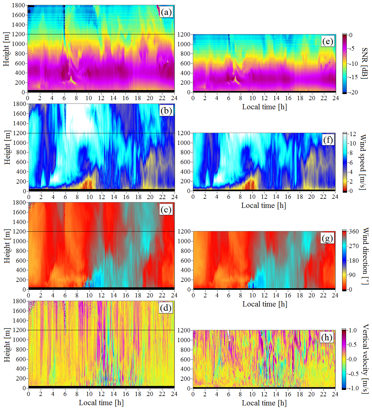
Figure 1Height–temporal distributions of the signal-to-noise ratio (a, e), wind speed (b, f), wind direction angle (c, g), and vertical component of the wind vector (d, h) for elevation angles of 60∘ (a–d) and 35.3∘ (e–h) on 21 July 2019.
From the obtained arrays of lidar estimates of the radial velocity and , the height–temporal distributions of the turbulence energy dissipation rate and the variance of radial velocity up to heights of 1200 m (i=1, elevation angle φ=35.3∘) and 1800 m (i=2, φ=60∘) were calculated by Eqs. (1)–(5). In the calculations with Eqs. (2) and (3), we took N=15. For scanning at two angles at Tscan=60 s, this corresponds to the approximately 30 min average of measured data. The calculated results are shown in Figs. 2 and 3. The black color in these figures and in Fig. 5 represents a lack of data because of their low quality owing to an insufficiently high signal-to-noise ratio (Banakh et al., 2017).
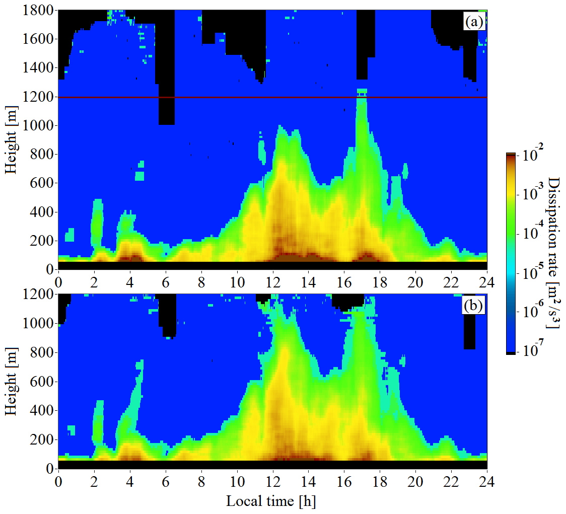
Figure 2Height and time distributions of the turbulence energy dissipation rate at elevation angles of 60∘ (a) and 35.3∘ (b). Measurements were taken on 21 July 2019.
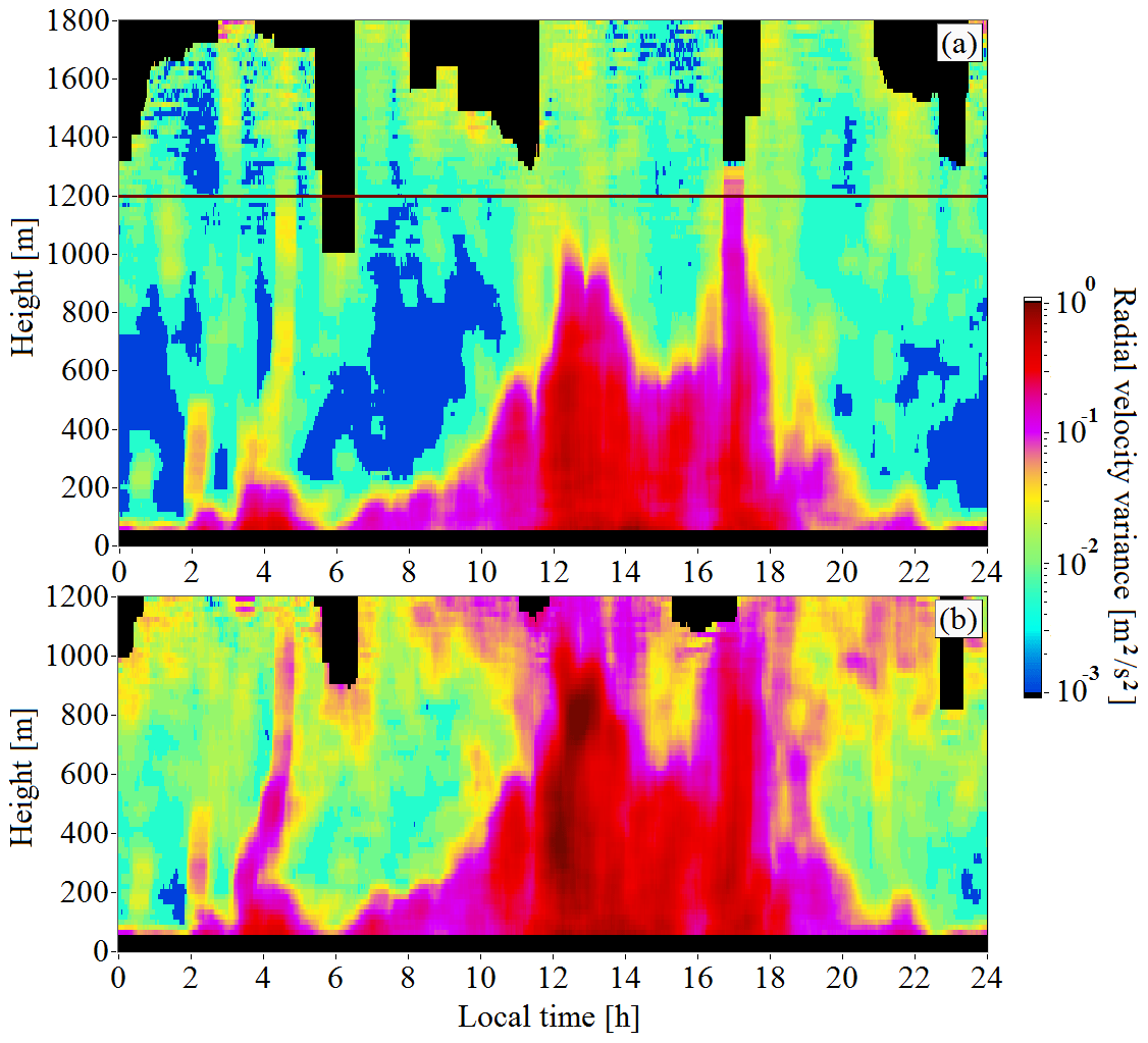
Figure 3Height and time distributions of the variance of radial velocity at elevation angles of 60∘ (a) and 35.3∘ (b). Measurements were taken on 21 July 2019.
A comparison of the data in Fig. 2a and b for the lower 1 km layer of the atmosphere demonstrates the closeness of the estimates ε1(h,t) and ε2(h,t) obtained from measurements at different elevation angles, which is in agreement with the results of Banakh and Smalikho (2019) and confirms the assumption of horizontal homogeneity of the turbulent wind field. The difference in the estimates of the radial velocity and measured at different elevation angles (see Fig. 3a and b) is more significant than that for the dissipation rate and is caused by the anisotropy of wind turbulence (Banakh and Smalikho, 2019).
The mixing layer height hmix was determined from the obtained height–temporal distributions of and for every instant with the use of the relations m2/s2 and m2/s3. The maximum height of the estimation of the temporal MLH series was 1.2 km for the measurements at an elevation angle of 35.3∘ and 1.8 km for the measurements at an angle of 60∘. The minimum height was h0=60 m. If the estimates of or at a height of 60 m were smaller than the corresponding threshold, we did not estimate the mixing layer height for such cases. If the estimates of or at the maximum height exceeded the threshold, we took hmix to be equal to the maximum height of retrieval of the vertical profiles of turbulence parameters.
Figure 4 shows the diurnal time series of obtained from the height–temporal distributions of the dissipation rate and the variance of radial velocity shown in Figs. 2 and 3. One can see that for the diurnal series of the turbulent mixing layer height retrieved from measurements of the dissipation rate at elevation angles of 35.3 and 60∘, we have, with rare exceptions, rather close results. The temporal series calculated from the variances differ more widely as a result of turbulence anisotropy (Banakh and Smalikho, 2019).
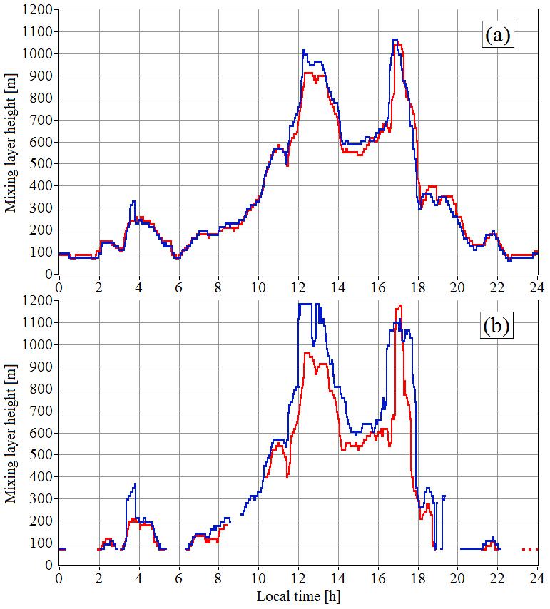
Figure 4Temporal series of the turbulent mixing layer height (thickness) obtained from spatiotemporal distributions of the turbulence energy dissipation rate (a) and the variance of radial velocity (b). Scanning at elevation angles of 60∘ (red curves) and 35.3∘ (blue curves). Measurements were taken on 21 July 2019. The data of Figs. 2 and 3 are used.
Since the temporal MLH series found from estimates of the dissipation rate at different elevation angles differ insignificantly, for other days of the experiment, we calculated from the estimates of the dissipation rate obtained by scanning at an elevation angle 60∘. The signal-to-noise ratio (SNR) at heights above 500 m is markedly higher at an elevation angle of 60∘ than at φ=35.3∘ (Fig. 1a and e). Thus, measurements at 60∘ provide an estimation of turbulence intensity at higher levels.
Figure 5 shows the height–temporal distributions over of the signal-to-noise ratio, wind velocity, wind direction angle, and turbulent energy dissipation rate, retrieved from lidar measurements during 6 d of the considered experiment. From the data for the SNR, it can be seen that in the morning hours of 20, 22, and 25 July, there was cloudiness at low heights, which rose over time due to convection. During the first 3 d of the experiment, the wind was predominantly northerly. From 11:00 to 19:00 UTC/GMT+7 on 21 July (see Fig. 1c and g, as well), the wind direction changed to the west, and there were significant changes in the wind direction with height, which is apparently the reason for the local minimum of the mixing layer height at about 15:00 UTC/GMT+7 (see Fig. 4). From about 12:00 UTC/GMT+7 on 23 July to 18:00 UTC/GMT+7 on 24 July the wind was predominantly southerly.
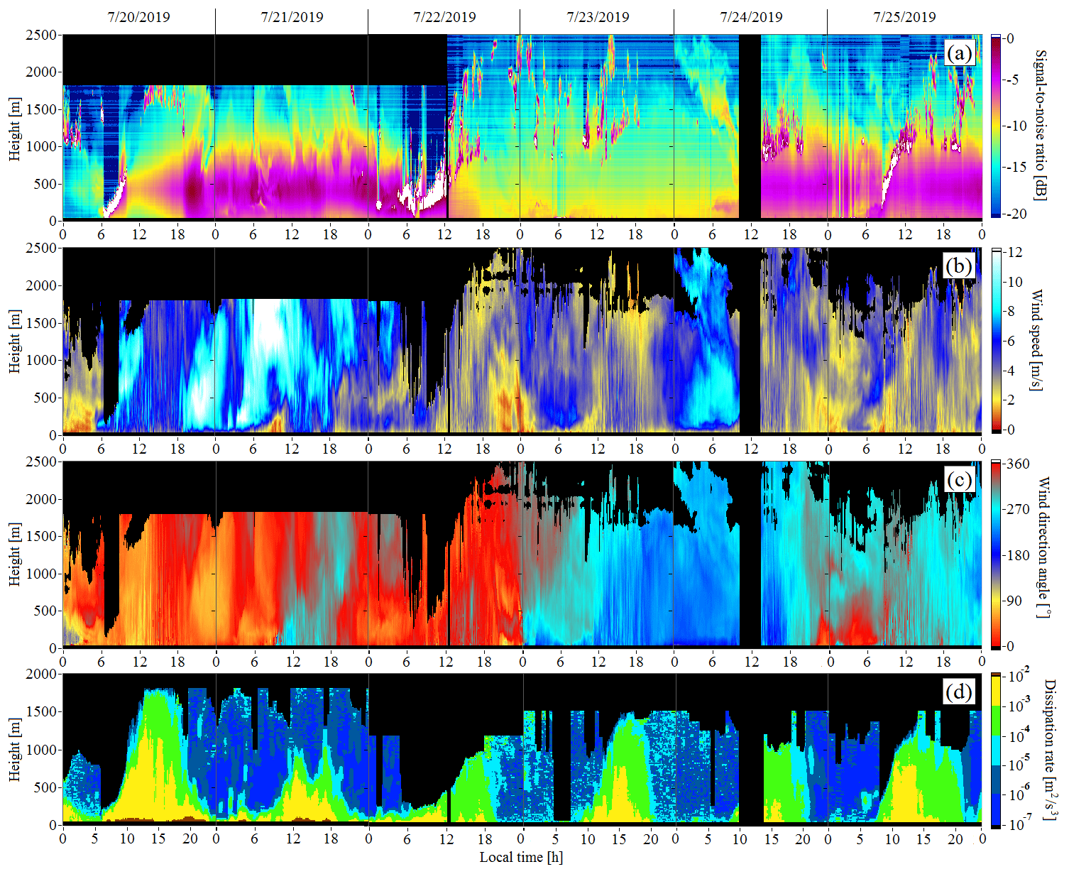
Figure 5Height and time distributions of SNR (a), wind speed (b), wind direction angle (c), and turbulent energy dissipation rate (d) retrieved from StreamLine lidar measurements at elevation angles of 60∘.
Using the data in Fig. 5 for the dissipation rate and the threshold m2/s3, we obtained the dependence of the height of the mixing layer on time during 6 d of the experiment (from 20 to 25 July 2019). The time series are shown in Fig. 6. One can see from Fig. 6 that on 20 and 25 July the time series of MLH are practically identical during the period from 08:00 to almost 12:00 UTC/GMT+7. In both cases, the increase in hmix was accompanied by the rise of the cloud base due to convection (see Fig. 5a for SNR). It follows from Fig. 6 that between 12:00 and 18:00 UTC/GMT+7 in the daytime, the mixing layer height varied widely between 400 and 1800 m.
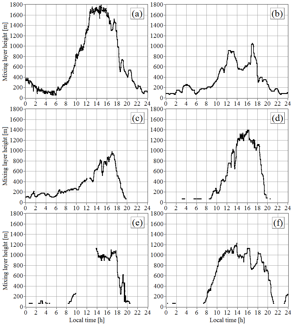
Figure 6Time series of the turbulent mixing layer height (thickness) obtained from lidar data on 20 July (a), 21 July (b), 22 July (c), 23 July (d), 24 July (e), and 25 July (f) of 2019.
From 00:00 to 07:00 UTC/GMT+7 in the morning and 21:00 to 24:00 UTC/GMT+7 in the evening, when the temperature stratification, according to data of sonic anemometers employed in this experiment, was stable, approximately in half of the cases the MLH could not been estimated, since the values of the dissipation rate at the lowest height (h0=60 m) were less than the threshold of 10−4 m2/s3. The choice of the minimum height h0=60 m in the measurements at the elevation angle φ=60∘ is explained by the fact that the minimum range of the pulsed coherent Doppler lidar should be no smaller than the two lengths of the probing volume (Smalikho et al., 2015). Used in the experiment range gate length ΔR=18 m corresponds to a 120 ns time window. Hence, according to calculations by Eq. (2.34) in Banakh and Smalikho (2013), the StreamLine lidar emitting 170 ns pulses formed a probing volume with a longitudinal dimension of 30 m.
The results shown in Fig. 6 do not contradict the known experimental data relative to estimates of the absolute values of the mixing layer height at different times of the day and night (Tucker et al., 2009; Barlow et al., 2011; Vakkari et al., 2015; Huang et al., 2017; Bonin et al., 2018; Manninen et al., 2018). Nevertheless, we made an attempt to determine the accuracy of the lidar estimate of the mixing layer height for conditions of this experiment.
The accuracy of MLH estimation from the PCDL data obtained with the use of conical scanning is determined by the error of estimation of the turbulence energy dissipation rate in the relatively thin atmospheric layer centered at the height hmix. To determine this error, we calculated not only height–temporal distributions of the dissipation rate but also instrumental errors of lidar estimation of the radial velocity by Eq. (23) from Smalikho and Banakh (2017). Then, the relative errors of lidar estimation of the turbulence energy dissipation rate %, where is the estimate and ε is true dissipation rate) were calculated with the use of the distributions of the dissipation rate and the instrumental error by Eqs. (6)–(11) from Banakh et al. (2017), and the time series of this error at heights were determined.
Figure 7 illustrates the behavior of the relative error for the diurnal time series of MLH shown in Fig. 6. It follows from Fig. 7a that the relative errors exceed 30 % for measurements on 20 July in the period between 00:00 and 06:00 UTC/GMT+7. This is explained by the relatively large instrumental error of estimation of the radial velocity due to the low signal-to-noise ratio ( dB, see Fig. 5a). On the same day, in the period between 11:00 and 18:00 UTC/GMT+7, the signal-to-noise ratio at heights above 1 km did not exceed −10 dB (Fig. 5a) and sometimes decreased to the lowest threshold dB, at which the probability of a bad (false) estimate of the radial velocity Pb can still be considered close to zero. As a result, the instrumental error of estimation of the radial velocity σe is much larger than that at heights below 1 km. As the mixing layer height increases, SNR decreases, and the error σe increases too (and vice versa for a decrease in hmix). This explains the initial increase in the relative error of estimation of the dissipation rate Eε and its subsequent decrease in the considered period between 11:00 and 18:00 UTC/GMT+7. In the other periods, as can be seen from Fig. 7a, the error Eε is about 10 %, which provides high accuracy of the determination of the mixing layer height.

Figure 7Relative error of estimation of the turbulent energy dissipation rate at the mixing layer heights determined from measurements on 20 July (a), 21 July (b), 22 July (c), 23 July (d), 24 July (e), and 25 July (f) of 2019.
On 21 July, the signal-to-noise ratio in the 1 km layer adjacent to the Earth's surface was very high most of the time (see Figs. 1a or 5a). Correspondingly, the instrumental error of estimation of the radial velocity σe within the mixing layer did not exceed 0.1 m/s. Therefore, according to the data in Fig. 7b, the error of estimation of the dissipation rate Eε(hmix) was low (mostly about 10 %) and did not exceed 18 %.
According to the data in Fig. 7c, the relative error of the dissipation rate estimates in the period 00:00 to 18:00 UTC/GMT+7 on 22 July did not exceed 25 %. This is due to the rather high signal-to-noise ratio at the top of the mixing layer (see Figs. 5a and 6c). On 23 July, the signal-to-noise ratio was low. Within the mixing layer, SNR is dB at a height of 100 m and dB at a height of 1 km (see Fig. 5a). As a result, the relative error Eε(hmix) varied widely from 10 % to 30 % (mostly larger than 15 %), as is indicated by Fig. 7d.
Due to the lack of measurement data on 24 July from about 10:00 to 13:30 UTC/GMT+7, and very weak turbulence on this day at night and in the evening, we calculated the relative errors in estimating the dissipation rate in a short period of time, as can be seen in Fig. 7e.
In the period between 08:00 and 20:40 UTC/GMT+7 on 25 July, as is seen in Fig. 7f, the dissipation rate was determined with very high accuracy. The relative error Eε(hmix) did not exceed 15 %, mostly 9 %, which is explained by the very high signal-to-noise ratio (see Fig. 5a). Despite the fact that the SNR was also rather high for the rest of the time, the accuracy of the dissipation rate estimation in the periods from 00:00 to 07:00 and from 21:00 to 23:00 UTC/GMT+7 on 25 July was low, and the relative error Eε(hmix) exceeded 30 %. The reason for this is that the dissipation rate at the height m during this time, according to Fig. 5a, was smaller by approximately an order of magnitude than the threshold value m2/s3.
With the use of the algorithm in Smalikho and Banakh (2013), we conducted a series of closed numerical experiments on the retrieval of vertical profiles of the turbulence energy dissipation rate ε(hk) from simulated lidar data. The purpose of these experiments is to reveal the degree of impact of the signal-to-noise ratio and the vertical gradient of the dissipation rate on the accuracy of estimating hmix by the proposed method. The simulation was performed for different values of the signal-to-noise ratio (SNR) and the vertical gradient of the dissipation rate at the height h, where the dissipation rate was set equal to m2/s3. The turbulent mixing layer height was estimated from the profiles of ε(hk) obtained in the numerical experiments with the use of the threshold m2/s3. The obtained estimates were compared with the preset values hmix. The analysis of results of the numerical experiments shows that the accuracy of estimates depends significantly not only on SNR but also on the vertical gradient of the dissipation rate γ. The smaller the value of γ (the slower the decrease in the dissipation rate with height), the larger the error .
Calculation of the error σh, using the data of the above experiment, with the algorithm in Smalikho and Banakh (2013), would require very computationally expensive simulation. The error of MLH estimation was determined in another way. To this end, on the assumption that Eε(hk)<30 %, the random estimate of the dissipation rate at the height hk was taken as
where ε(hk) and Eε(hk) are respectively the estimate of the dissipation rate and its relative error obtained from the data of the lidar experiment, and ξ(hk) is a pseudo-random number obeying the Gaussian statistics with zero mean 〈ξ〉=0 and unit variance 〈ξ2〉=1. To construct the vertical profile , random numbers ξ(hk) for different heights hk were generated in accordance with the correlation function , where hmix is the turbulent mixing layer height determined from the atmospheric experiment, , and Δh=15.6 m is a step in height at ΔR=18 m and φ=60∘. The correlation function Cξ(lΔh) was found from averaging of random realizations of at the values of hmix and SNR observed in the experiment (Figs. 5a, d, 6). For the error Eε(hk)<30 % and m2/s3, the correlation function Cξ(lΔh) weakly depends on SNR and hmix, which considerably simplifies the procedure of numerical simulation of by Eq. (6).
Let us consider an example of calculating the error in estimating the height of the mixing layer from the lidar data of an atmospheric experiment. Figure 8 shows the altitude profiles of the signal-to-noise ratio, the instrumental error in estimating the radial velocity, the relative error in estimating the rate of dissipation, and the dissipation rate itself. Data were taken from lidar measurements from 17:40 to 18:20 UTC/GMT+7 on 20 July 2019. It can be seen that in a layer up to 1400 m the signal-to-noise ratio is so high that the instrumental error in estimating the radial velocity and the relative error in estimating the dissipation rate do not exceed 0.3 m/s (Fig. 8b) and 30 % (Fig. 8c), respectively. According to Fig. 8d, the point of intersection of the vertical profile ε(hk) of the threshold m2/s3 is at a height hmix=976 m. At this height, the vertical gradient of the dissipation rate m/s3.
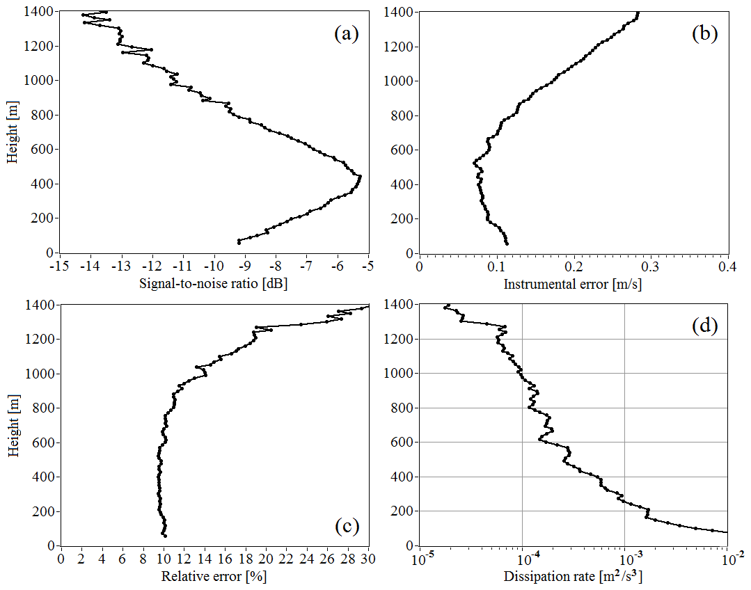
Figure 8Vertical profiles of signal-to-noise ratio (a), instrumental error of radial velocity estimate (b), relative error of estimation of the turbulent energy dissipation rate (c), and turbulent energy dissipation rate (d) retrieved from measurements from 17:40 to 18:20 on 20 July 2019.
Figure 9 shows (as red curves) statistically independent random realizations of vertical profiles of the dissipation rate simulated by Eq. (6) using the data in Fig. 8c (Eε(hk)) and Fig. 8d (ε(hk)). The estimates of the mixing layer height determined from each of the simulated profiles are given in Fig. 9 as well. Using 100 000 independent estimates , we found that the error in estimating the height of the mixing layer σh=69 m.
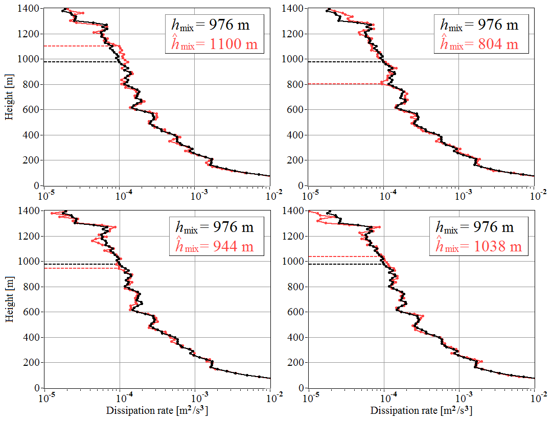
Figure 9Measured (black curve taken from Fig. 8d) and four examples of random realizations of simulated (red curves obtained with the use of Eq. 6 and data of Fig. 8c and d) vertical profiles of the turbulent energy dissipation rate.
Figure 10 shows the errors in the estimates of the mixing layer height obtained from lidar measurements during 6 d of the experiment (from 20 to 25 July 2019). The figure shows that, depending on the atmospheric conditions (signal-to-noise ratio and the vertical gradient of the dissipation rate), the error in the lidar estimate of the mixing layer height varies from 10 to 100 m or more. Even with a very high SNR and small error of estimation of the dissipation rate, the error can exceed 100 m due to the small value of the vertical gradient of the dissipation rate γ (see data in Figs. 5a and d, 7f, and 10f for the time interval 19:00–20:00 UTC/GMT+7 on 25 July 2019).
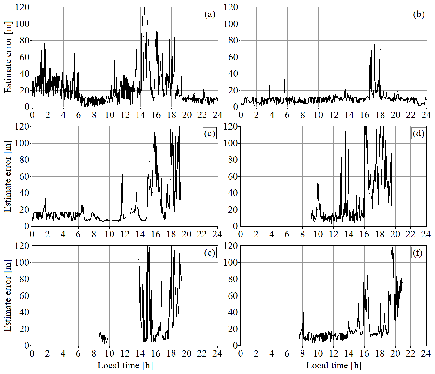
Figure 10Error of estimation of the mixing layer heights determined from measurements on 20 July (a), 21 July (b), 22 July (c), 23 July (d), 24 July (e), and 25 July (f) of 2019.
Calculations of the relative error % of lidar estimation of the turbulent mixing layer height, carried out using the data in Figs. 6 and 10, showed that, with rare exceptions, Eh does not exceed 30 %, and for data measured from 12:00 to 18:00 UTC/GMT+7, Eh varies from 2 % to 10 %. It should be noted that the relative error Eh does not exceed 20 % if the estimate of the mixing layer height is obtained from lidar measurements with SNR of at least −16 dB.
One of the parameters characterizing the stability of the atmospheric boundary layer is the gradient Richardson number,
where
is the potential temperature, T(h,t) is the temperature of the air, γa=0.0098 ∘/m is the dry-adiabatic lapse rate, and . The gradient Richardson number can be used to estimate the turbulent mixing layer height (Helmis et al., 2012; Petenko et al., 2019; Gibert et al., 2011).
For additional proof of the suitability of the method for estimating the turbulent mixing layer height from lidar data obtained with the use of conical scanning, we conducted a lidar experiment with concurrent measurement of the temperature. The experiment was conducted from 8 April to 6 May 2020. The temperature was measured by the MTP-5 microwave temperature profiler (Atmospheric Technology, Dolgoprudny, Moscow, Russia). This profiler is widely used in atmospheric research currently. The accuracy of temperature measurement and experience of the use of this device in the atmospheric boundary layer research is discussed in references 51–58 cited in Banakh et al. (2020). The temperature profiler and the wind lidar StreamLine were installed on the roof of the Institute of Atmospheric Optics (IAO) building in Tomsk (56.475504∘ N, 85.048225∘ E) 4 km from the Basic Experimental Observatory. The profiler provided measurements of the vertical temperature profiles every 5 min, with a resolution of 25 m for heights from 0 to 100 m and a resolution of 50 m for heights from 100 to 1000 m with respect to the height of its installation. As a result, we obtained the height–temporal distributions of the air temperature T(h,t). In calculating the derivative and the parameter N2 (Eq. 8), we used the temperature measurement data averaged over a 10 min period. Then, the Richardson number Ri was calculated by Eq. (7). The mean horizontal wind velocity U and its derivative in Eq. (7) were assessed from the lidar data averaged, as with the temperature, over a 10 min period (10 scans). The parameters and geometry of the lidar measurements were the same as those in July 2019. The scanning was carried out at an elevation angle of 60∘.
In contrast to uniquely high SNR for lidar StreamLine in July 2019, during this experiment the signal-to-noise ratio was rather low. It did not allow us to obtain estimates of the wind velocity with an acceptable error at heights above 800 m–1 km. The conditionSNR dB, which provides an acceptable error in estimating the dissipation rate by the method used (Smalikho and Banakh, 2017), was violated at heights above 400 m. As a consequence, the relative errors of estimation of the turbulence energy dissipation rate and the turbulent mixing layer height could exceed 30 % starting from heights of 400 m. Moreover, the weather was rainy and snowy during the experiment often, and not all the measurement data could be used in processing. Nevertheless, the height–temporal distributions of the dissipation rate obtained in the experiment allowed us to monitor the turbulent mixing layer height by the threshold m2/s3 in many cases.
Figure 11 shows the daily height–temporal distributions of the turbulence energy dissipation rate and the Richardson number assessed from the data of wind velocity and temperature measurements on 10, 12, 15, 21, 22, 26, and 27 April and on 1 May 2020. The distributions illustrate typical stratification regimes which were observed in the atmospheric boundary layer during the experiment. White curves in Fig. 11 show the diurnal time series of the turbulent mixing layer height, as estimated from the threshold value m2/s3 for the turbulence energy dissipation rate. Red curves in Fig. 11 show the diurnal time series of the SNR at the level −16 dB. Black color on the Richardson number distributions in Fig. 11 shows the zones where Ri<0.5.
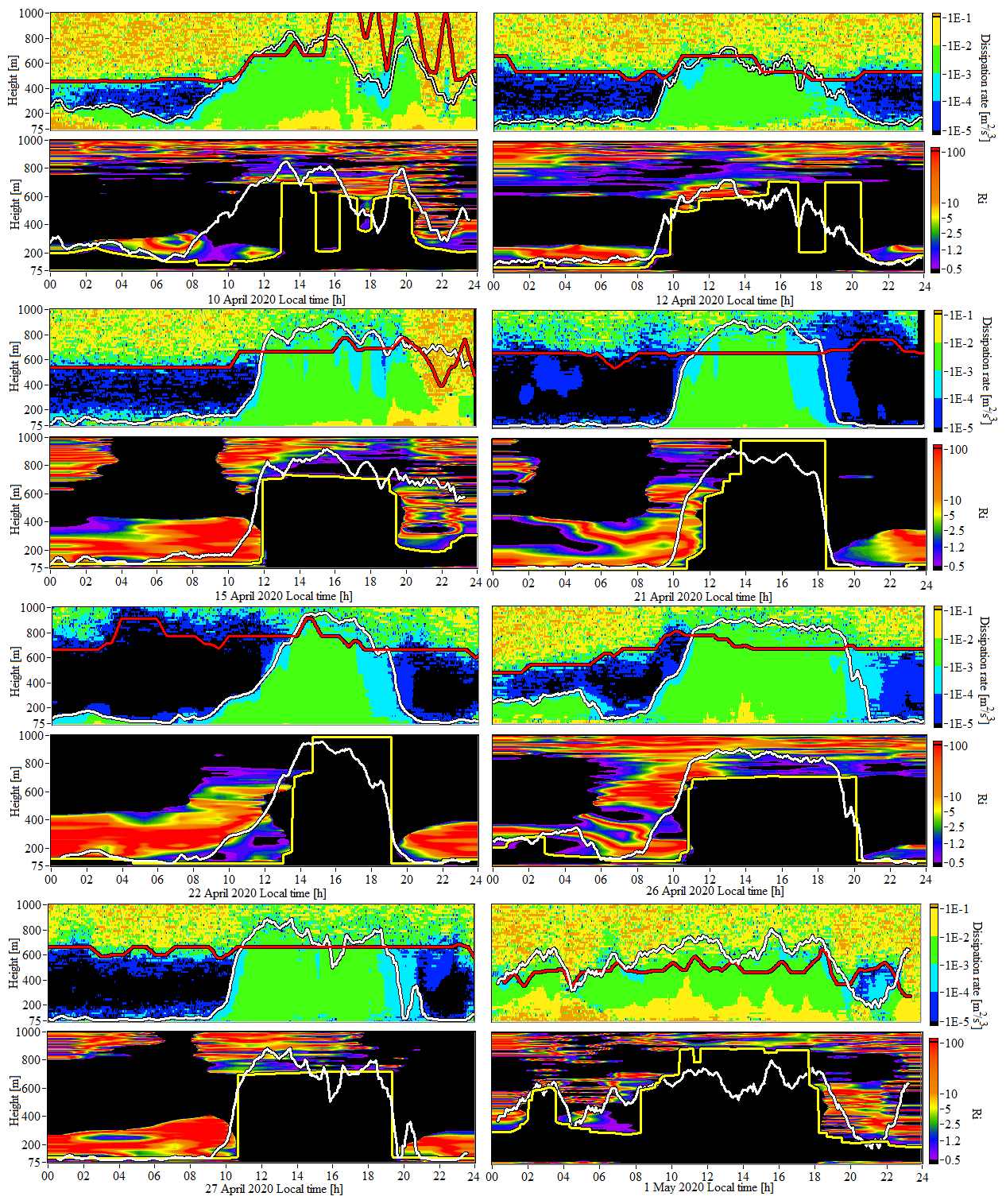
Figure 11Height–temporal distributions of the turbulence energy dissipation rate and the Richardson number as obtained from measurements on 10, 12, 15, 21, 22, 26, and 27 April and on 1 May 2020. White curves reproduce the diurnal time series of the turbulent mixing layer height, as estimated from the turbulence energy dissipation rate. Red curves show the diurnal time series of the SNR at the level −16 dB. Black color on the Richardson number distributions shows the zones where Ri<0.5. Yellow curves show the diurnal time series of the turbulent mixing layer height, estimated as a minimum height, above which the Richardson number exceeds 0.5.
When estimating the daily variations in the height of the turbulent mixing layer from the height–temporal distributions of the Richardson number, we considered the following. According to the classification of the atmospheric turbulent regimes based on the Richardson number (Baumert and Peters, 2009; Grachev et al., 2013), the small-scale turbulence becomes weak at gradient Richardson numbers more than 0.5. Therefore, it is natural to believe that the turbulent mixing occurs at the time and heights at which the Richardson number Ri<0.5. Thus, the minimum height, above which the Richardson number exceeds 0.5, can be taken as the height of the turbulent mixing layer at the current time moment. Yellow curves show the diurnal time series of the turbulent mixing layer height hmixR, as estimated from the distributions of the Richardson number using this criterion.
The temporal variations of the MLH estimated from the dissipation rate of turbulence energy reproduce the development of the turbulence in the daytime observed from the height–temporal distributions of the Richardson number on 15, 21, 26, and 27 April 2020 with good accuracy. For these days in the period between 12:00 and 18:00 UTC/GMT+7 the estimates of the MLH based on the dissipation rate hmix (white curves) differ from the MLH estimates calculated based on the Richardson number hmixR (yellow curves) insignificantly. The relative divergence of the heights hmix and hmixR, determined as , is less than 25 % on average in these periods.
The criterion used for determining hmixR is sensitive to the small spots with Ri>0.5 against the background areas with Ri<0.5, while the estimates of the MLH based on the dissipation rate do not “notice” them. It is the reason for the strong divergence of hmix and hmixR in the morning hours on 10, 12, 21, 22, and 26 April and on the 1 May. This is also a reason for the strong divergence of hmix and hmixR in the afternoon on 10 and 12 April.
Thus, from Fig. 11 it follows that the estimates of the turbulent mixing layer height as a height at which the dissipation rate becomes less than the threshold value m2/s3, and as a height above which the Richardson number exceeds 0.5, are in a qualitative agreement.
In this paper, we propose a method for estimating the turbulent mixing layer height on the basis of the height–temporal distributions of the turbulence energy dissipation rate obtained from PCDL measurement data with conical scanning by a probing beam around the vertical axis. The method was tested in the experiments in summer 2019 in strong smog due to forest fires and in spring 2020.
The optical characteristics of the atmosphere varied significantly during the experiment in 2019. Most of the time, the aerosol backscatter coefficient far exceeded the background level because of the smog. Under these conditions, the signal-to-noise ratio (SNR) was abnormally high for lidars in the class of the StreamLine lidar with a pulse energy of about 10 µJ. As a result, in the experiment, we succeeded in retrieving the vertical profiles of the wind speed and direction up to a height of 2.5 km and wind turbulence parameters up to a height of 1.8 km.
The raw data of the lidar experiments conducted on 20–25 July 2019 were used to find the diurnal time series of MLH under conditions of intense smog from the height–temporal distributions of the dissipation rate with the use of the inequality m2/s3 as a criterion that indicates the absence of turbulent mixing. According to the results obtained, on these days, the MLH was at its maximum between 11:00 and 18:00 UTC/GMT+7 and varied from 400 to 1800 m. It was shown in the experiment that the estimation of the turbulent mixing layer height from the height–temporal distributions of the turbulence energy dissipation rate has some advantages in comparison with the estimation from the height–temporal distributions of the variance of radial velocity. Because of the anisotropy of wind turbulence, the variance of radial velocity depends significantly on the elevation angle of the scanning.
The accuracy of the method for estimating the turbulent mixing layer height from the lidar data obtained with the use of conical scanning is discussed in detail in this paper. We developed a method for calculating the experimental error of estimation of the turbulent mixing layer height from the height–temporal distributions of the turbulence energy dissipation rate. The analysis of the errors calculated by this method shows that the accuracy of MLH estimation depends decisively on the error of estimation of the dissipation rate and on the vertical gradient of the dissipation rate at heights near the top of the mixing layer. In turn, the accuracy of estimation of the dissipation rate depends strongly on the lidar signal-to-noise ratio (SNR). For the estimation of MLH with the acceptable relative error not exceeding 20 %, SNR should be no less than −16 dB, when the relative error of lidar estimation of the dissipation rate does not exceed 30 %. With the data obtained in the experiments, we demonstrate that the relative error of determination of the MLH time series from lidar measurements of the dissipation rate with the use of conical scanning does not exceed 10 % in the period of turbulence development, from 06:00 to 22:00 UTC/GMT+7. Most of the time in this period, it is less 5 %. The method described here can be applied to data measured by a high-power pulsed coherent Doppler lidar at a background aerosol concentration, which will enable a full-edged statistical analysis.
To prove the suitability of the method for estimating the turbulent mixing layer height from lidar data obtained with the use of conical scanning, we conducted a lidar experiment with concurrent measurement of the temperature in April–May 2020. From the obtained data, we calculated the height–temporal distributions of the gradient Richardson number and determined the MLH from these distributions. A comparison shows that the estimates of the turbulent mixing layer height from the dissipation rate distributions and from the Richardson number distributions using the criterion Ri<0.5 are in a qualitative agreement.
All the data presented in this study are available from the authors upon request.
VAB led the experiment, analyzed the data, and wrote the manuscript. INS built the software, led numerical analysis, analyzed the data, participated in the field work, and contributed to the manuscript. AVF led the experiment and built the software. All authors have read and agreed to the submitted version of the manuscript.
The authors declare that they have no conflict of interest.
The authors are thankful to Artem Sherstobitov for helping with data processing. The authors thank the reviewers for invaluable contribution in improvement of the manuscript.
This research has been supported by the Russian Science Foundation (grant no. 19-17-00170).
This paper was edited by Laura Bianco and reviewed by two anonymous referees.
Banakh, V. and Smalikho, I.: Coherent Doppler Wind Lidars in a Turbulent Atmosphere, Artech House Publishers, Boston and London, ISBN: 13-978-1-60807-667-3, 2013.
Banakh, V. A. and Smalikho, I. N.: Lidar studies of wind turbulence in the stable atmospheric boundary layer, Remote Sens., 10, 1219, https://doi.org/10.3390/rs10081219, 2018.
Banakh, V. A. and Smalikho, I. N.: Lidar estimates of the anisotropy of wind turbulence in a stable atmospheric boundary layer, Remote Sens., 11, 2115, https://doi.org/10.3390/rs11182115, 2019.
Banakh, V. A., Smalikho, I. N., and Falits, V. A.: Estimation of the turbulence energy dissipation rate in the atmospheric boundary layer from measurements of the radial wind velocity by micropulse coherent Doppler lidar, Opt. Express, 25, 22679–22692, https://doi.org/10.1364/OE.25.022679, 2017.
Banakh, V. A., Smalikho, I. N., and Falits, A. V.: Wind–Temperature Regime and Wind Turbulence in a Stable Boundary Layer of the Atmosphere: Case Study, Remote Sens., 12, 955, https://doi.org/10.3390/rs12060955, 2020.
Barlow, J. F., Dunbar, T. M., Nemitz, E. G., Wood, C. R., Gallagher, M. W., Davies, F., O'Connor, E., and Harrison, R. M.: Boundary layer dynamics over London, UK, as observed using Doppler lidar during REPARTEE-II, Atmos. Chem. Phys., 11, 2111–2125, https://doi.org/10.5194/acp-11-2111-2011, 2011.
Baumert, H. Z. and Peters, H.: Turbulence closure: turbulence, waves and the wave-turbulence transition – Part 1: Vanishing mean shear, Ocean Sci., 5, 47–58, https://doi.org/10.5194/os-5-47-2009, 2009.
Bonin, T. A., Carroll, B. J., Hardesty, R. M., Brewer, W. A., Hajny, K., Salmon, O. E., and Shepson, P. B.: Doppler lidar observation of the mixing height in Indianapolis using an automated composite fuzzy logic approach, J. Atmos. Ocean. Tech., 35, 915–935, https://doi.org/10.1175/JTECH-D-17-0159.1, 2018.
Eberhard, W. L., Cupp, R. E., and Healy, K. R.: Doppler lidar measurement of profiles of turbulence and momentum flux, J. Atmos. Ocean. Tech., 6, 809–819, 1989.
Emeis, S., Schafer, K., and Munkel, C.: Surface-based remote sensing of the mixing-layer height – a review, Meteorol. Z., 17, 621–630, 2008.
Frehlich, R. G. and Yadlowsky, M. J.: Performance of mean-frequency estimators for Doppler radar and lidar, J. Atmos. Ocean. Tech., 11, 1217–1230, 1994.
Garratt, J. R.: The atmospheric boundary layer, Cambridge atmospheric and space science series, Cambridge University Press, Cambridge, 1994.
Gibert, F., Arnault, N., Cuesta, J., Plougonven, R., and Flamant, P. H.: Internal gravity waves convectively forced in the atmospheric residual layer during the morning transition, Q. J. Roy. Meteor. Soc., 137, 1610–1624, 2011.
Grachev, A. A., Andreas, E. L., Fairall, Ch. W., Guest, P. S., Ola, P., and Persson, G.: The Critical Richardson Number and Limits of Applicability of Local Similarity Theory in the Stable Boundary Layer, Bound.-Lay. Meteorol., 147, 51–82, https://doi.org/10.1007/s10546-012-9771-0, 2013.
Helmis, C. G., Sgouros, G., Tombrou, M., Schäfer, K., Münkel, C., Bossioli, E., and Dandou, A.: A Comparative Study and Evaluation of Mixing-Height Estimation Based on Sodar-RASS, Ceilometer Data and Numerical Model Simulations, Bound.-Lay. Meteorol., 145, 507–526, https://doi.org/10.1007/s10546-012-9743-4, 2012.
Hogan, R. J., Grant, A. L. M., Illingworth, A. J., Pearson, G. N., and O'Connor, E. J.: Vertical velocity variance and skewness in clear and cloud-topped boundary layers as revealed by Doppler lidar, Q. J. Roy. Meteor. Soc., 135, 635–643, https://doi.org/10.1002/qj.413, 2009.
Huang, M., Gao, Z., Miao, S., Chen, F., Lemone, M. A., Li, J., Hu, F., and Wang, L.: Estimate of boundary-layer depth over Beijing, China, using Doppler lidar data during SURF-2015, Bound.-Lay. Meteorol., 162, 503–522, https://doi.org/10.1007/s10546-016-0205-2, 2017.
Manninen, A., Marke, T., Tuononen, M., and O'Connor, E.: Atmospheric boundary layer classification with Doppler lidar, J. Geophys. Res., 123, 8172–8189, https://doi.org/10.1029/2017JD028169, 2018.
O'Connor, E. J., Illingworth, A. J., Brooks, I. M., Westbrook, C. D., Hogan, R. J., Davies, F., and Brooks, B. J.: A method for estimating the kinetic energy dissipation rate from a vertically pointing Doppler lidar, and independent evaluation from balloon-borne in situ measurements, J. Atmos. Ocean. Tech., 27, 1652–1664, https://doi.org/10.1175/2010JTECHA1455.1, 2010.
Petenko, I., Argentini, S., Casasanta, G., Genthon, C., and Kallistratova, M.: Stable Surface-Based Turbulent Layer During the Polar Winter at Dome C, Antarctica: Sodar and In Situ Observations. Bound.-Lay. Meteorol., 171, 101–128, https://doi.org/10.1007/s10546-018-0419-6, 2019.
Pichugina, Y. L. and Banta, R. M.: Stable boundary layer depth from high-resolution measurements of the mean wind profile, J. Appl. Meteorol. Clim., 49, 20–35, 2010.
Schween, J. H., Hirsikko, A., Löhnert, U., and Crewell, S.: Mixing-layer height retrieval with ceilometer and Doppler lidar: from case studies to long-term assessment, Atmos. Meas. Tech., 7, 3685–3704, https://doi.org/10.5194/amt-7-3685-2014, 2014.
Smalikho, I. N.: Techniques of wind vector estimation from data measured with a scanning coherent Doppler lidar, J. Atmos. Ocean. Tech., 20, 276–291, 2003.
Smalikho, I. N. and Banakh, V. A.: Accuracy of Estimation of the Turbulent Energy Dissipation Rate from Wind Measurements with a Conically Scanning Pulsed Coherent Doppler Lidar. Part I. Algorithm of Data Processing, Atmos. Ocean. Opt., 26, 404–410, 2013.
Smalikho, I. N. and Banakh, V. A.: Measurements of wind turbulence parameters by a conically scanning coherent Doppler lidar in the atmospheric boundary layer, Atmos. Meas. Tech., 10, 4191–4208, https://doi.org/10.5194/amt-10-4191-2017, 2017.
Smalikho, I. N., Banakh, V. A., Holzäpfel, F., and Rahm, S.: Method of radial velocities for the estimation of aircraft wake vortex parameters from data measured by coherent Doppler lidar, Opt. Express, 23, A1194–A1207, https://doi.org/10.1364/OE.23.0A1194, 2015.
Stull, R. B.: An introduction to boundary layer meteorology, Kluwer Academic Publishers, Dordrecht, the Netherlands, 1988.
Tucker, S. C., Brewer, W. A., Banta, R. M., Senff, C. J., Sandberg, S. P., Law, D. C., Weickmann, A. M., and Hardesty, R. M.: Doppler lidar estimation of mixing height using turbulence, shear, and aerosol profiles, J. Atmos. Ocean. Tech., 26, 673–688, 2009.
Vakkari, V., O'Connor, E. J., Nisantzi, A., Mamouri, R. E., and Hadjimitsis, D. G.: Low-level mixing height detection in coastal locations with a scanning Doppler lidar, Atmos. Meas. Tech., 8, 1875–1885, https://doi.org/10.5194/amt-8-1875-2015, 2015.
- Abstract
- Introduction
- Method for determination of the turbulent mixing layer height from PCDL data obtained by conical scanning
- Experiment during forest fires in Siberia in 2019
- Results of the experiment
- Error of MLH estimation
- Comparison with the Richardson number
- Summary
- Data availability
- Author contributions
- Competing interests
- Acknowledgements
- Financial support
- Review statement
- References