the Creative Commons Attribution 4.0 License.
the Creative Commons Attribution 4.0 License.
 | 01 Mar 2021
Satellite imagery and products of the 16–17 February 2020 Saharan Air Layer dust event over the eastern Atlantic: impacts of water vapor on dust detection and morphology
Lewis Grasso
Daniel Bikos
Jorel Torres
John F. Dostalek
Ting-Chi Wu
John Forsythe
Heather Q. Cronk
Curtis J. Seaman
Steven D. Miller
Emily Berndt
Harry G. Weinman
Kennard B. Kasper
On 16–17 February 2020, dust within the Saharan Air Layer (SAL) from western Africa moved over the eastern Atlantic Ocean. Satellite imagery and products from the ABI on GOES-16, VIIRS on NOAA-20, and CALIOP on CALIPSO, along with retrieved values of layer and total precipitable water (TPW) from MIRS and NUCAPS, respectively, were used to identify dust within the SAL over the eastern Atlantic Ocean. Various satellite imagery and products were also used to characterize the distribution of water vapor within the SAL. There was a distinct pattern between dust detection and dust masking and values of precipitable water. Specifically, dust was detected when values of layer TPW were approximately 14 mm; in addition, dust was masked when values of layer TPW were approximately 28 mm. In other words, water vapor masked infrared dust detection if sufficient amounts of water vapor existed in a column. Results herein provide observational support to two recent numerical studies that concluded water vapor can mask infrared detection of airborne dust.
- Article
(17125 KB) - Full-text XML
- BibTeX
- EndNote


For over 45 years, satellite data have been used to detect airborne dust. Detection of dust has been explored with the use of low earth orbiting (LEO) sensors such as the (i) Moderate Resolution Imaging Spectroradiometer (King et al., 1992), (ii) Cloud-Aerosol Lidar with Orthogonal Polarization (CALIOP; Winker et al., 2009), and (iii) Temperature Humidity Infrared Radiometer and Image Dissector Camera System (both onboard Nimbus-4; Shenk and Curran, 1974). In addition, geostationary sensors such as the (i) Spinning Enhanced Visible and InfraRed Imager (SEVIRI) onboard METEOSAT Second Generation (MSG) (Schmetz et al., 2002) and (ii) Advanced Baseline Imager (ABI; Kalluri et al., 2018; Schmit et al., 2008) onboard GOES-16/17 have been used to explore dust. Platforms orbiting the Earth allowed for many types of techniques to detect airborne dust.
Typically, several types of procedures exist that use a variety of spectral bands to detect dust in the atmosphere of the Earth. For example, Ashpole and Washington (2012), Knippertz and Todd (2010), Torres et al. (1998, 2007), and Herman et al. (1997) used spectral bands in the ultraviolet for dust detection. In addition, techniques have also been developed that required only spectral bands in the infrared (Lensky and Rosenfeld, 2008; Chaboureau et al., 2007; Darmenov and Sokolik, 2005; Ackerman, 1997; Legrand et al., 1989; Shenk and Curran, 1974). There also exist dust detection algorithms that use a combination of spectral bands that detect both solar reflection and infrared energy (Cho et al., 2013; Zhao et al., 2010; Hao and Qu, 2007; Pierangelo et al., 2004; Miller, 2003; Miller et al., 2017; Legrand et al., 2001; Tanre and Legrand, 1991; Ackerman, 1989). Of the above studies, some have speculated about the relationship between water vapor and dust detection.
An open question centers on the interdependence of water vapor and dust detection algorithms. Although each of the above studies focused on examining which spectral bands may be used for dust detection, a few did raise the question of possible effects, either advantageously or adversely, of water vapor on dust detection (Ashpole and Washington, 2012; Knippertz and Todd, 2010; Chaboureau et al., 2007; Legrand et al., 2001; Tanre and Legrand, 1991). Interestingly, Pierangelo et al. (2004), pointed out that dust interfered with temperature and water vapor retrievals. Recent work, however, directly addressed the impact water vapor may have on dust detection.
Therefore, the statement of the problem in this paper is that two recent studies explored the use of numerical modeling to support an hypothesis that water vapor has the ability to mask dust (Banks et al., 2019; Miller et al., 2019). This paper examines an observational case of the Saharan Air Layer (SAL; Prospero and Carlson, 1972; Adams et al., 2012; Dunion and Velden, 2004; Kuciauskas et al., 2018) dust event over the eastern Atlantic Ocean. Results of the 16–17 February 2020 observational study serve to support Banks et al. (2019) and Miller et al. (2019) by showing that reduced values of water vapor allowed dust associated with the SAL to be both detected and tracked over the eastern Atlantic Ocean. Observational datasets include (1) a simple difference in infrared imagery, (2) a microwave retrieval of layer precipitable water known as the Advected Layer Precipitable Water (ALPW) product (Forsythe et al., 2015; LeRoy et al., 2016), and (3) an infrared retrieval of total precipitable water (TPW; Gambacorta and Barnet, 2013; Gambacorta, 2013), all of which addressed water vapor in the environment of dust within the SAL.
Organization of the paper is as follows: a detailed discussion of sources of satellite and retrieved data is found in Sect. 2. An in-depth examination and interpretation of dust within the SAL as revealed by remote imagery is the focus of Sect. 3. Assimilation of dust is a relatively new effort; as such, a brief overview of recent efforts of dust assimilation are contained in Sect. 4. National Weather Service forecasters provide pertinent forecasting issues and potential impacts associated with dust events associated with the SAL over southern Florida in Sect. 5, which is entitled “Forecaster perspective”. Finally, the summary and conclusions are provided in Sect. 6.
Satellite data from three sources and retrieved precipitable water from two sources were used for this study. Satellite data were acquired from the (1) Advanced Baseline Imager (ABI) onboard the Geostationary Operational Environmental Satellite (GOES)-16, (2) Visible Infrared Imaging Radiometer Suite (VIIRS) onboard the National Oceanic and Atmospheric Administration (NOAA)-20, and (3) Cloud-Aerosol Lidar with Orthogonal Polarization (CALIOP) onboard the Cloud–Aerosol Lidar Infrared Pathfinder Satellite Observation (CALIPSO). Retrieved precipitable water was acquired from (1) the NOAA Unique Combined Atmospheric Processing System (NUCAPS) and (2) the Microwave Integrated Retrieval System (MIRS). Although this paper focuses on a dust plume associated with the SAL that moved from western Africa to the eastern Atlantic Ocean, the lack of a blue band (∼0.47 µm) on SEVIRI, which is onboard MSG-11, whose sub-point is the intersection of the prime meridian and the Equator, prevents the generation of Geo/True-Color imagery. As a result, discussions about the airborne dust will utilize the above sources. A brief discussion of each data source will be discussed presently; additional information may be found in the included references.
On 19 November 2016, GOES-R was launched from Kennedy Space Center, Cape Canaveral, Florida. After reaching a position at 89.5∘ W and undergoing a check-out period, the satellite assumed an operational identification of GOES-16 and currently resides at 75.2∘ W. Imagery from ABI, one of the primary sensors on GOES-16, was used for this study. Unlike previous GOES imagers, ABI collects imagery at 16 different spectral bands with a nadir footprint of 0.5, 1.0, and 2.0 km (Kalluri et al., 2018; Schmit et al., 2008; Goodman et al., 2012). There are several applications for data from ABI, e.g., GeoColor imagery (Miller et al., 2016, 2017), cloud properties (Heidinger et al., 2015), land and ocean surfaces, the cryosphere, atmospheric soundings, and atmospheric aerosol (Schmit et al., 2017, 2018). Additional information about GOES-16 and other satellites in the GOES-R series may be found in Goodman et al. (2019).
VIIRS was first placed on the Suomi National Polar-orbiting Partnership (S-NPP) platform, which was launched on 28 October 2011. S-NPP served as a demonstration, as opposed to an operational satellite. Due to the success of S-NPP, VIIRS was placed onboard the Joint Polar Satellite System (JPSS) (Goldberg et al., 2013). On November 2017, JPSS-1 was launched; the satellite assumed the operational identification of NOAA-20 on 18 November 2018. Both S-NPP and NOAA-20 are in the same orbital plane and are separated by approximately half an orbit, allowing for two VIIRS images every ∼50 min. VIIRS allows for imaging of footprints at both 750 m for M-bands and 375 m for I-bands. VIIRS swath widths are approximately 3000 km; further, VIIRS contains a day–night band, which has the ability to capture several features at night due to reflected moonlight and surface light sources. A detailed list of applications and capabilities of VIIRS are discussed in Hillger et al. (2013, 2014) and Miller et al. (2012, 2013).
On 28 April 2006, CALIPSO was launched and positioned in the A-Train constellation of low Earth orbiting satellites. CALIOP (Winker et al., 2009) is the main sensor onboard CALIPSO. CALIOP, a lidar, emits packets of 110 mJ of energy at a frequency of 20.25 Hz downward to the surface of the Earth. In addition, backscattered energy is detected at 532 nm, polarized 532 nm, and 1064 nm by three detectors on the satellite; additional details are described in Hunt et al. (2009). CALIOP acquires data that are used to produce the Vertical Feature Mask (VFM). VFM is a vertically oriented plane within which certain atmospheric constituents, if present, are identified. Some of the identifiable constituents are clear sky, clouds, and aerosols (Liu et al., 2005). CALIOP differs from ABI and VIIRS; specifically, both ABI and VIIRS are passive sensors while CALIOP is an active sensor.
Retrieved atmospheric soundings of temperature and water vapor were acquired from the NOAA Unique Combined Atmospheric Processing System (NUCAPS; Gambacorta and Barnet, 2013; Gambacorta, 2013), which is a NOAA operational algorithm for hyperspectral infrared retrievals. A modular algorithm design allows NUCAPS to be applied to hyperspectral infrared sounders on multiple satellite platforms. In the case of the S-NPP/NOAA-20 series of satellites, NUCAPS uses input from the Cross-track Infrared Sounder and the Advanced Technology Microwave Sounder sensors. NUCAPS also uses cloud-cleared radiances and an iterative regularized least-squares minimization algorithm to produce vertical profiles of temperature and water vapor from microwave and infrared radiances. A total of 30 retrievals are performed across a 2200 km swath, with footprint sizes ranging from ∼50 km at nadir to 70 km×134 km at the edge. Retrieved profiles are mapped onto 100 vertical levels between 1100 and 0.016 hPa. Examples of applications include finding the “Cold-air aloft” aviation hazard (Weaver et al., 2019), assessing the pre-convective environment and retrieved atmospheric stability (Iturbide-Sanchez et al., 2018; Bloch et al., 2019; Esmaili et al., 2020), assessing changes in the intensity of both midlatitude cyclones and hurricanes (Berndt et al., 2016; Berndt and Folmer, 2018), and evaluating retrieved soundings for a variety of atmospheric moisture regimes, including regions impacted by the Saharan Air Layer (Nalli et al., 2016; Kuciauskas et al., 2018).
NUCAPS vertical temperature and moisture soundings were first introduced to National Weather Service forecasters in 2014. Since then, satellite sounding products have been adapted and expanded in response to end-user feedback (Esmaili et al., 2020). Plan-view and cross section display capabilities (i.e., Gridded NUCAPS; Berndt et al., 2020) are one example of a capability developed to facilitate the use of NUCAPS in the operational environment and enable its use for new applications. NUCAPS temperature, moisture, ozone, and derived fields such as TPW are mapped to a 0.5∘ grid with minimal horizontal interpolation utilizing nearest neighbor and vertically interpolated to standard meteorological levels. Although TPW is not derived by the NUCAPS algorithm, values are calculated with the standard TPW equation whereby water vapor mixing ratio is vertically integrated from the surface to the top of a sounding to represent the depth of condensed water vapor in an atmospheric column.
Layer precipitable water (LPW) is the depth of condensed water vapor that exists between two given pressure levels. An initial LPW product (Forsythe et al., 2015; LeRoy et al., 2016) was developed at CIRA, which employed a fusion of the NOAA MIRS (Boukabara et al., 2011) water vapor profile retrievals from seven LEO satellites. Satellites used in the initial LPW study were S-NPP, NOAA-19/20, MetOp-A/B, and Defense Meteorological Satellite Program F17/18. Advection of retrieved LPW utilizes winds from the Finite Volume Cubed Global Forecast System (FV3GFS, hereafter GFS) to create Advected Layer Precipitable Water (ALPW), which uses a technique called advective blending (Gitro et al., 2018). ALPW is computed within the following four pressure layers: (1) the surface to 850 hPa, (2) 850–700 hPa, (3) 700–500 hPa, and (4) 500–300 hPa. Computation of the ALPW takes place at CIRA and is created hourly with a 16 km footprint. ALPW allows forecasters to (1) track the movement of water vapor within several layers and (2) determine the availability of moisture for heavy precipitation events. ALPW complements water vapor depictions from both geostationary platforms and numerical weather prediction models. Because ALPW is derived from passive microwave measurements, retrievals are available in the presence of clouds, which is in contrast to infrared-based retrievals, such as NUCAPS. Water vapor retrievals from MIRS have no dependence on dynamic forecast models, which allows for independent comparison to model analyses and forecasts.
In order to display both satellite data and retrieved soundings, this study utilized the Advanced Weather Interactive Processing System (AWIPS). AWIPS was used for the GOES-R satellite product demonstration, which included a variety of weather applications (Goodman et al., 2012). As such, both ABI and VIIRS satellite imagery, along with NUCAPS and ALPW products presented herein, were processed with AWIPS. Further, data transmitted to AWIPS via the Satellite Broadcast Network have a 6 km footprint on the full disk sector; an exception is GeoColor imagery, which is mapped to a 1.5 km grid and available in AWIPS from CIRA via a Local Data Manager feed. Lower resolution or latency of the full disk sector was suited for imagery of dust within the SAL because the 16–17 February 2020 SAL will be shown to be a slowly evolving feature. Because low latency was not an issue for slowly evolving features, dust within the SAL was a phenomena that was also well suited to imagery and products from polar-orbiting satellites.
During the day of 16 February 2020, a relatively large area of dust associated with the SAL moved westward from western Africa to the eastern Atlantic Ocean. Because there are a dearth of observations over western Africa and the eastern Atlantic Ocean, this study employed the GFS analyses, or zero-hour forecast, to provide supplemental meteorological information. Superimposed on GOES-16 GeoColor imagery (Miller et al., 2016, 2020) valid at 18:00 UTC on 16 February 2020 (Fig. 1) was an inverted trough (Schlueter et al., 2019) at 700 hPa, indicated by a the geopotential heights and a dashed black contour positioned over the eastern Atlantic. Associated with the inverted trough was a thermal minimum at 700 hPa, which was positioned just west of the trough axis. Temperatures at the center of the thermal minimum were the lowest in the scene with values near 0 ∘C and increased to the southwest to values near 6 ∘C. Dust existed in a region that was roughly bounded by the 315 and 318 dm geopotential height contours, to the east by the axis of the inverted trough, and to the southwest by the 6 ∘C isotherm.
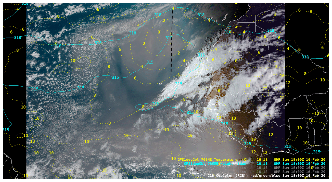
Figure 1GeoColor imagery derived from ABI on GOES-16 along with the (1) 315 dm and 318 dm 700 hPa geopotential height (solid contour) and (2) 700 hPa isotherms (∘C, dashed contour) from the GFS analysis. A dashed black contour is used to denote the axis of an inverted trough. All data are valid at 18:00 UTC 16 February 2020.
There was an ascending CALIPSO overpass located over the eastern Atlantic Ocean for the dust case discussed herein. Data from CALIOP provided information about the field of aerosols evident in Fig. 1. In Fig. 2a, the orbit of CALIPSO, denoted by a green line segment, entered the scene along the southern portion of the image at approximately 15:30 UTC 16 February 2020, moved towards the northwest, and exited the scene at approximately 15:43 UTC 16 February 2020. As stated in Sect. 2, the VFM provides information about atmospheric constituents in a vertical plane. One of the constituents was aerosol, which was further sub-classified into four aerosol types: dust, polluted continental, polluted dust, and smoke. As can be seen in Fig. 2b, there were two sub-aerosol types in the lower atmosphere from the surface to approximately 3.0 km over a significant portion of the orbit in Fig. 2a. North of approximately 15∘ N, the VFM suggested dust was the primary constituent in the aerosol layer. However, the VFM suggested a significant portion of the aerosol layer, south of 15∘ N, was occupied not only by dust but also by polluted dust; i.e., dust was ubiquitous for the entire transect, with the greatest pollution concentrations found south of 15∘ N.
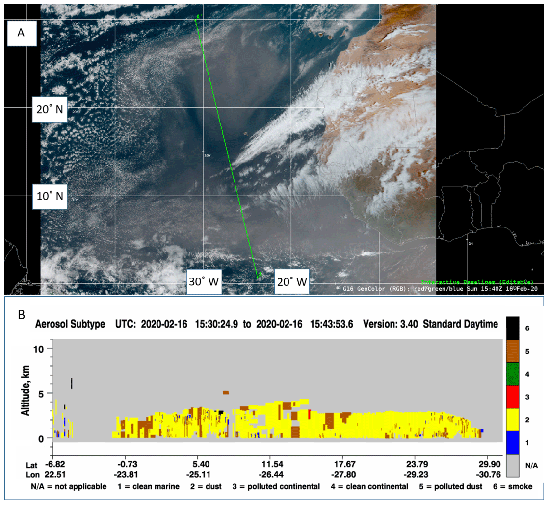
Figure 2(a) GeoColor imagery derived from ABI on GOES-16 valid at 15:40 UTC 16 February 2020, along with a portion of the ground track (green line segment) of CALIPSO from 15:30 to 15:43 UTC 16 February 2020. (b) Retrieved aerosol subtype is displayed in the vertical feature mask from CALIOP.
Although data contained in the VFM image of Fig. 2b is a vertical cross section along the orbital path of CALIPSO, a few assumptions are made herein. One assumption is that all aerosol in the region north of approximately 15∘ N and west of the inverted trough in Fig. 1 was dust and will be referred to as the northern dust region (NDR). Further, a second assumption is that all aerosol in the region south of about 10∘ N and west of Africa was a mixture of polluted dust and dust and will be referred to as the southern dust region (SDR).
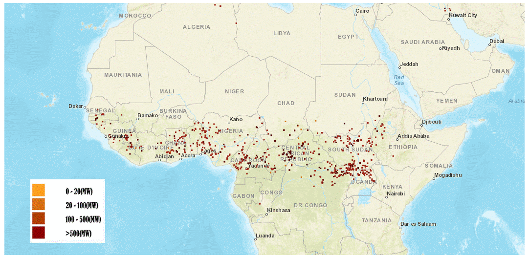
Figure 3VIIRS active fire map (VAFM) for 15 February 2020, 1 d prior to the dust case study herein. Dots indicate the locations of burning while the color of the dots denotes values of the fire radiative power. Credit is given to the VAFM group for the image.
Two questions arise about the aerosol layer in Fig. 2. First, can an inference be made about the vertical depth of the entire dust field based on the VFM? Results from Adams et al. (2012) provides a climatology of the vertical depth of dust associated with the SAL, which suggests in the months December, January, and February that dust layers from western Africa are about 2.0 to 3.0 km thick (see their Fig. 3c), which is consistent with Fig. 2b. Second, examination of Fig. 2a exhibits an east–west layer of aerosol south of about 10∘ N. Is there a source of pollution that can help explain the existence of polluted dust south of 10∘ N in Fig. 2a and b? One possible candidate is smoke from biomass burning along equatorial Africa.
One of the products from the VIIRS instrument is the VIIRS Active Fire Map (VAFM) (Csiszar et al., 2014). A plot of the VAFM from 15 February 2020, 1 d prior to the dust case discussed herein, is displayed in Fig. 3. Regions of active fire were indicated by dots of varying colors; each color represents a range of values of the fire radiative power, which can be used to estimate emissions from biomass burning (Ahmadov et al., 2017). Biomass burning occurred in the latitudinal range from the Equator to about 10∘ N over Africa. This paper speculates that smoke from burning on 15 February 2020, indicated in Fig. 3, may be the source of pollution of the polluted dust retrieved by CALIOP south of 10∘ N in Fig. 2b.
There were two main regions of aerosol in satellite imagery on 16 February 2020. To begin with, a black oval is used in Fig. 4 to demarcate the NDR seen in GeoColor imagery from ABI onboard GOES-16; similarly, the SDR is denoted by a broken, east–west, black line segment in Fig. 4. There are also a few additional annotation symbols in Fig. 4 that will be discussed shortly.
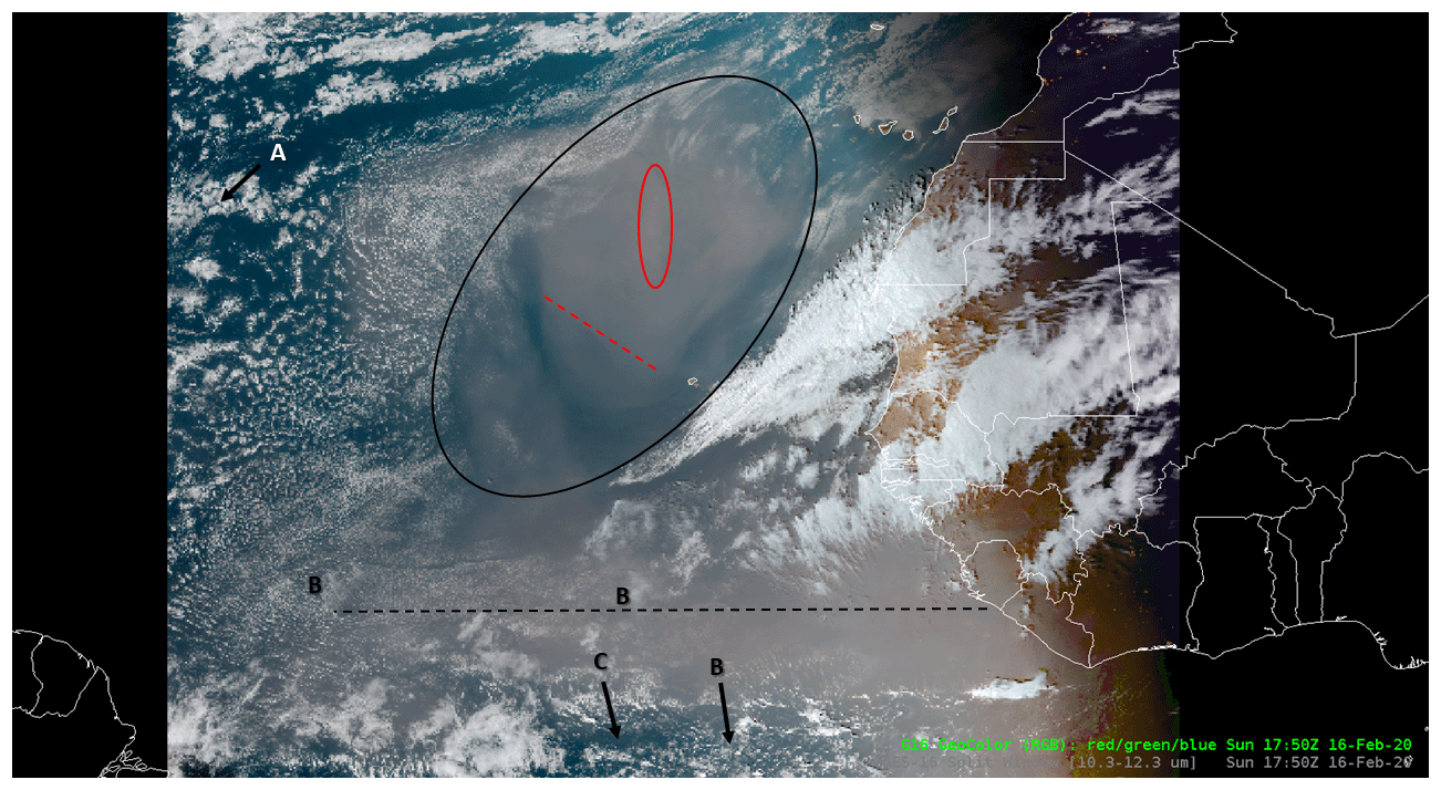
Figure 4GeoColor imagery derived from ABI on GOES-16, valid at 18:00 UTC 16 February 2020, along with the following annotations: a black oval bounds dust in the northern dust region. while the horizontal dashed black line highlights dust in the southern dust region. Within the black oval are additional annotations in red. Further, the letters A (upper-left portion of the figure), B, and C show locations referred to in the text.
As mentioned in Sect. 1, channel differencing of infrared channels has been used at times to identify lofted dust. In a study by Miller et al. (2019), several numerical experiments were used to examine channel differencing of infrared wavelengths and dust detection. Specifically, plots of values of brightness temperatures (Tbs) at 12.3 µm subtracted from values of Tbs at 10.35 µm, Tb(10.35 µm) − Tb(12.3 µm), were shown to be negative for airborne dust, with a caveat: vertically integrated values of water vapor had to be below some critical value. In contrast, if values of water vapor in a layer, which also contained dust, exceed a critical integrated amount, then values of the channel difference were shown to be positive. Although GeoColor imagery is a novel way to display imagery (Fig. 4), horizontal variations of vertically integrated water vapor have little impact on such imagery. Horizontal variations of vertically integrated water vapor do impact channel differencing between Tbs at 12.3 and 10.35 µm, which is displayed in Fig. 5, valid at 18:00 UTC 16 February 2020.

Figure 5Channel difference, Tb(10.35 µm) − Tb(12.3 µm) (∘C), from ABI on GOES-16, valid at 18:00 UTC 16 February 2020. Annotations are the same as in Fig. 4. Dust is indicated by the blue and purple colors within the black oval in the northern dust region. There was a lack of a dust signal in the southern dust region.
Most of the region bounded by the black oval in Fig. 5 had values of the channel difference near zero (blue) and less than zero (purple). A word of caution is warranted: in general, a functional mapping between an atmospheric feature and a value of the ABI channel difference Tb(10.35 µm) − Tb(12.3 µm) does note exist. In other words, there is no inverse mapping from a value in the channel difference to a unique atmospheric feature. For example, low-level liquid water clouds and dust were both mapped to values that were near zero or negative, while thin cirrus and relatively moist boundary layers were both mapped to relatively large positive values (orange or red).
Physical interpretation of values in the channel difference image was be done by direct comparison with a GeoColor image. Two features appeared blue in Fig. 5; one feature was within the black oval, while another was located in the upper-left portion of the figure, which is denoted by a white colored letter A. A direct comparison of these features between the GeoColor image in Fig. 4 and the channel difference in Fig. 5 suggested that the blue color within the oval (Fig. 5) was associated with the dust plume (Fig. 4), while the blue color in the upper left of Fig. 5 was associated with low-level liquid water clouds in Fig. 4. Note the difference in the appearance of the edge of the blue regions in Fig. 5. This indicates that dust had a boundary that appeared diffuse; however, liquid water clouds had a rather sharp contrast with the environment at their boundary in Fig. 5. There were also two features that appeared orange or red in Fig. 5. One feature was located slightly above the middle and left edge of the broken horizontal black line segment, denoted by the letter B along with a region along the lower edge of the figure; also denoted with a letter B and arrow. Both orange and red features were barely discernable in Fig. 4 as they were thin cirrus. A second feature was located along the bottom of Fig. 5, denoted by the letter C, and appeared as a somewhat homogeneous orange color, which was coincident with clear skies in Fig. 4. Physical interpretation served to illustrate the lack of a functional mapping between an atmospheric feature and a value of the channel difference. This manuscript will now focus on the dust plume as seen in black oval exhibited in Figs. 4 and 5.
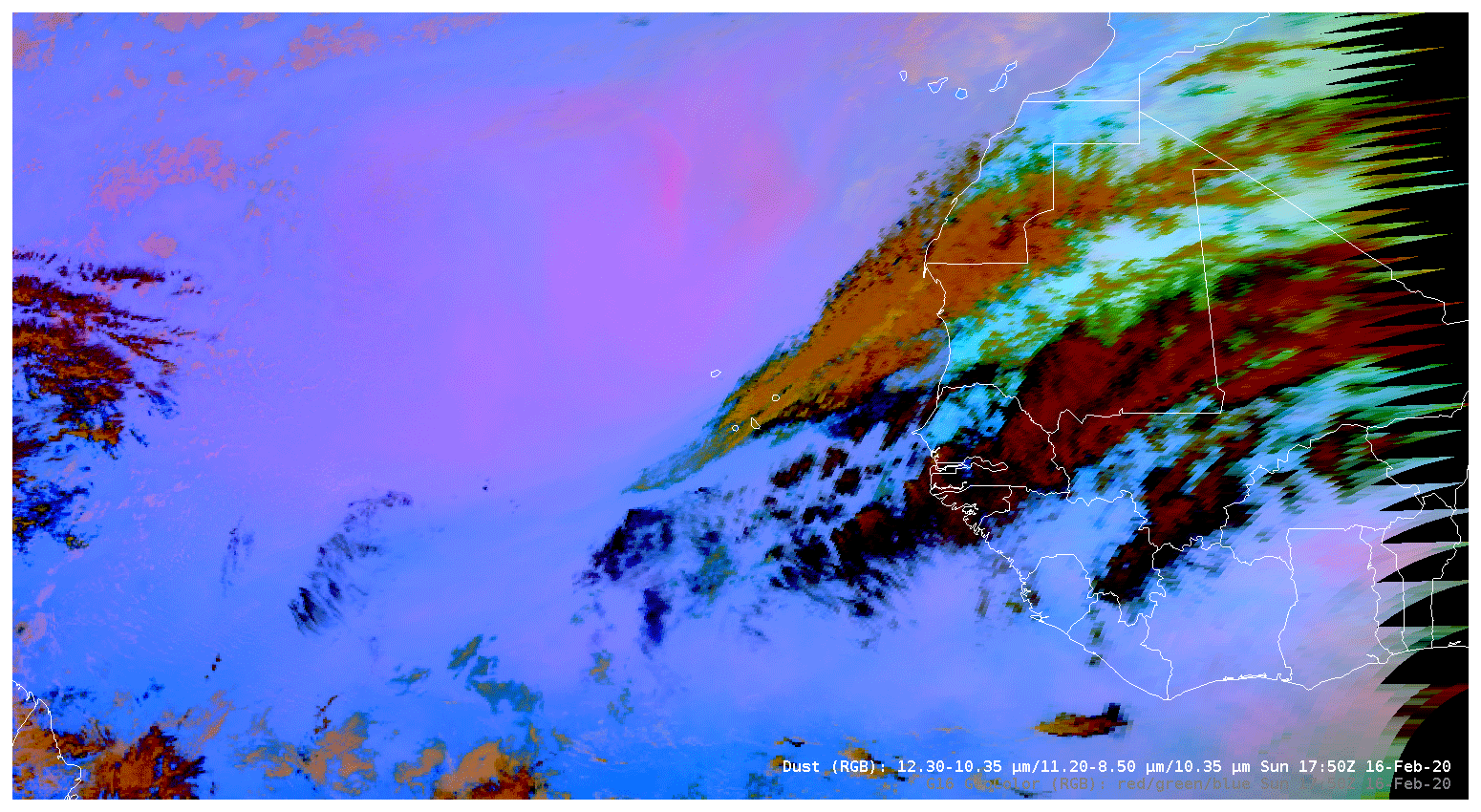
Figure 6SEVIRI dust product generated by using ABI bands on GOES-16 on 18:00 UTC 16 February 2020. A pink color, indicating dust, was characteristic of the northern dust region, while a blue color was characteristic of the southern dust region; i.e., dust within the southern dust region was less obvious.
Additional annotations appear within the black oval of Figs. 4 and 5. To begin with, the red oval in Fig. 4 bounded a north–south region of dust. Just to the northwest and southeast of the red oval, GeoColor imagery exhibited a touch of blue, suggesting that the dust was unable to obscure the ocean when compared to the region of dust within the red oval. A similar pattern was evident in the colors of the channel difference (Fig. 5). The region within the oval contained negative values (blue or purple) of the channel difference while just to the northwest and southeast of the red oval positive values (green) appeared. Similarly, there was an additional subtle touch of blue within the dust field to the southwest of the broken red line segment in Fig. 4 compared to regions to the northeast of the broken red line segment within the black oval. Similarly, increased values of the channel difference (blue/green) existed to the southwest of the broken line segment while smaller values (blue) existed to the northeast of the segment in Fig. 5. That the horizontal variability of appearance of dust in the black oval of Fig. 4 corresponded to a similar horizontal variability of values of the channel difference in the black oval of Fig. 5 supported the assumption that the blue and purple regions within the black oval in Fig. 5 were in response to the dust seen in Fig. 4. Note the lack of a dust signal along the broken east–west black line segment in Fig. 5; i.e., values of the channel difference were positive with values near 3 to 4 ∘C.
Although the Tb(10.35 µm) − Tb(12.3 µm) channel difference is a component of a dust product, there are other components. A dust product, which was developed for the SEVIRI instrument onboard MSG (Ashpole and Washington, 2012), was adapted to ABI bands for the dust case herein. Tbs from three of the ABI bands were used to generate the SEVIRI dust product: 8.5, 10.35, and 12.3 µm. A multi-color image was generated by assigning values of Tb(12.3 µm) − Tb(10.35 µm) to red, Tb(11.20 µm) − Tb(8.5 µm) to green, and Tb(10.35 µm) to blue (Fig. 6). As a result of the SEVIRI dust recipe, dust is indicated by a pinkish color. Due to differences in the spectral width and central wavelength of ABI bands compared to SEVIRI bands, the color component thresholds were adapted to account for the differing spectral characteristics and maintain the appearance of the dust product generated with ABI bands compared to SEVIRI bands (Shimizu, 2015; Berndt et al., 2018). For example, the ABI band centered near 10.35 µm has a spectral width from 10.1 to 10.6–0.5 µm; in contrast, the SEVIRI band centered near 10.80 µm has a spectral width from 9.8 to 11.8–2.0 µm. Further, the spectral width for the SEVIRI band centered near 10.80 µm exhibits an overlap with the SEVIRI band centered near 12.0 µm, which has a spectral width from 11.0 to 13.0 µm.
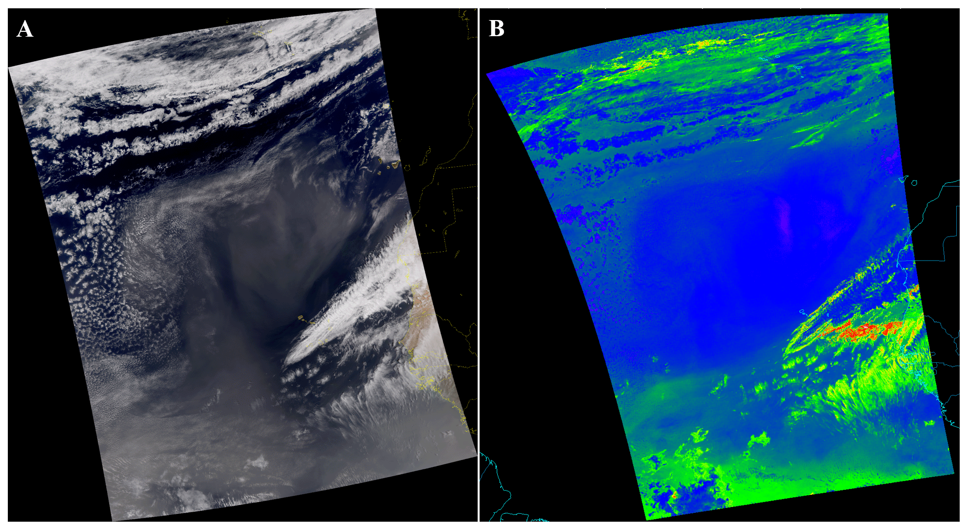
Figure 7Data from VIIRS on NOAA-20, valid at approximately 15:10 UTC 16 February 2020, showing (a) True-Color, as opposed to GOES-16 ABI GeoColor, imagery and (b) VIIRS channel difference, Tb(10.76 µm) − Tb(12.01 µm), with the same color table shown in Fig. 5.
As stated earlier, the channel difference Tb(10.35 µm) − Tb(12.3 µm) is used in dust detection algorithms. Consequently, horizontal variations evident in the NDR in Fig. 5 were also evident in Fig. 6. One of the assumptions stated above was that all aerosol north of approximately 15∘ N and west of the inverted trough, the NDR in Fig. 4, was dust. An examination of the NDR in Fig. 6 exhibited bright pink colors, which provided support for the first hypothesis. A second assumption stated that all aerosol south of about 10∘ N and west of Africa was a mixture of smoke and dust, the SDR in Fig. 4. In contrast to the NDR, an examination of the SDR in Fig. 6 exhibited mostly blue colors with a few hints of pink in some regions. Even though CALIOP data suggested dust in the SDR, support for the second hypothesis, based on results in Fig. 6, is less obvious. A question arises: why was there higher confidence of dust in the NDR compared to the SDR?
There was also a NOAA-20 overpass in the region of interest at approximately 15:10 UTC 16 February 2020, just prior to the CALIPSO overpass. As a reminder, GeoColor imagery from ABI is produced from the following three bands: 0.47, 0.64, and 0.87 µm. These three bands are then used to diagnose values of green reflectances; GeoColor imagery is produced by combining the ABI red, diagnosed green, and ABI blue bands. Because VIIRS measures radiances within the red, green, and blue regions of the electromagnetic spectrum, a True-Color, as opposed to GeoColor, image was produced for the dust case herein (Fig. 7a). Although the VIIRS True-Color image was captured near 15:10 UTC, there existed a similarity of aerosol features to the 18:00 UTC ABI GeoColor image in Figs. 1, 2, and 4. Although there was a nearly 3 h difference between the VIIRS and ABI images, the similarity of the aerosol features suggested a relatively slow temporal morphology of dust in the NDR and SDR.
VIIRS also contains bands from which the channel difference, a companion to Fig. 5, was generated. In Fig. 7b, the channel difference is shown with the same color table in Fig. 5. A comparison between Figs. 5 and 7b reveals that, despite the same color table, the two-channel difference images were different. While the channel difference in Fig. 5 was made with Tb(10.35 µm) − Tb(12.3 µm), the channel difference in Fig. 7b was made with Tb(10.76 µm) − Tb(12.01 µm). Therefore, the central wavelengths used in the channel difference for ABI and VIIRS were different. Further, the spectral widths of each band were also different. For example, the ABI spectral width for Tbs near 10.35 µm ranged from 10.1 to 10.6 µm; the VIIRS spectral width for Tbs near 10.76 µm ranged from 10.26 to 11.26 µm. Qualitatively, interpretation of the horizontal pattern of values of the channel difference in Fig. 7b were similar to the interpretation of Fig. 5. Thus, the NDR was characterized by values of the channel difference that were less than zero while the SDR was characterized by positive values of the channel difference. In other words, there was more of a dust signal in the NDR compared to the SDR.
In addition to dust, smoke from biomass burning over Africa (Fig. 3) existed within the SDR. One open question is whether smoke impacts values of Tb(10.35 µm) − Tb(12.3 µm) in such a way as to mask the dust in the SDR. Based on previous satellite observations, Hillger and Ellrod (2003) have shown that smoke layers were undetected in values of infrared channel differences. In an attempt for this paper to provide a more complete background of satellite detection of smoke, we note that Hillger and Ellrod (2003) also showed that if a layer of smoke is optically thick enough in infrared bands, Tbs of smoke will appear cool and may be confused with cool, elevated, land surfaces. As part of a discussion of the utility of the day–night band on the VIIRS sensor, Miller et al. (2013) also point out the inability of smoke detection by infrared satellite imagery. One consequence of these two studies suggests that smoke within the SDR was unable to mask dust in the SDR. Another mechanism for dust masking in the SDR is sought. Banks et al. (2019) and Miller et al. (2019) explored the question about dust masking; results from their numerical studies suggested that water vapor in excess of a critical value may mask dust.
Efforts will now focus on vertically integrated tropospheric water vapor for the scene in Fig. 1. There are measurements from ABI on GOES-16 that are in response to vertically integrated water vapor: Band 10, which detects upwelling radiation centered near 7.34 µm and is referred to as the low-level water vapor band. Low-level water vapor imagery at 18:00 UTC 16 February 2020 is displayed in Fig. 8. In the low-level water vapor image, maximum values of Tbs were in the yellow region with values near −2 ∘C. Values of Tbs decreased to near −15 ∘C in the region of red and then continued to decrease to values near −18 ∘C in regions of orange. In particular, values of Tbs decreased from approximately −2 ∘C (yellow) to −18 ∘C (orange) both north and south of the Tb maximum; Tbs decreased about 15 ∘C from the Tb maximum to the north-northeast and southeast. Was the decrease in values of Tbs of the low-level water vapor image due to horizontal variations of air temperature?

Figure 8Tb(7.34 µm) from ABI on GOES-16, color shaded with a few numerical values, along with TPW (mm; white contours) from the GFS analysis and a few values of Tb(7.34 µm) in black. All data are valid at 18:00 UTC 16 February 2020.
Brightness temperatures in the low-level water vapor image are presently compared to air temperatures. Because the weighting function for 7.34 µm imagery generally peaks at pressures greater than approximately 500 hPa (Schmit et al., 2018), air temperatures from 700 to 500 hPa were examined. Isotherms at 700 and 500 hPa, from the GFS zero-hour forecast, were plotted on ABI 7.34 µm imagery; all data was valid at 18:00 UTC 16 February 2020 (Fig. 9). As seen in Fig. 9, values of the air temperature at 700 and 500 hPa were approximately 8 and −7 ∘C, respectively, near the maximum value of Tbs near 7.34 µm (yellow). Values of the air temperature then decreased to near 6 and −11 ∘C, respectively, to the north-northeast of the Tb max, where values of the Tb were near −18 ∘C. Likewise, values of the air temperature at 700 and 500 hPa increased from about 8 and −7 ∘C to near 10 and −4 ∘C, respectively, to the southeast of the Tb maximum. Note the lateral change in values of Tbs were approximately 15 ∘C; in contrast, the lateral change in values of the 700 and 500 hPa air temperature were, in absolute value, about 2 and 4 ∘C, respectively. As a reminder, one characteristic of the tropical atmosphere is that geopotential variations and horizontal temperatures gradients are relatively small (Holton, 1979). Consequently, lateral changes in air temperature were unable to explain the lateral changes in Tbs and thus another reason was sought.

Figure 9The same as Fig. 8, except contoured values of 700 hPa (solid) and 500 hPa (dashed) temperatures (∘C) from the GFS analysis are plotted; all data are valid at 18:00 UTC 16 February 2020.
Values of TPW from the GFS are shown in relation to various satellite fields. In Fig. 8, values of TPW were plotted on the low-level water vapor image; both valid at 18:00 UTC 16 February 2020. In general, regions with the smallest values of TPW corresponded to regions with the largest values of Tbs in the low-level water vapor image. However, notice that the region to the north northeast of the Tb maximum, values of Tbs were approximately −19 ∘C in a location with values of the TPW near 19 mm. In contrast, values of Tbs to the southeast of the Tb maximum were also near −19 ∘C; however, values of TPW were approximately double with values about 38 mm. One possible reason for greater values of TPW to the southeast of the Tb maximum, compared to the north northeast of the Tb maximum, was that more water vapor existed below the peak of the weighting function for 7.34 µm. Thus, values of boundary layer water vapor decreased from regions to the southeast of the Tb maximum to regions to the north northeast of the Tb maximum. Values of analyzed surface dew point temperatures from GFS at 18:00 UTC 16 February 2020 suggested that values of dew point temperatures decreased from near 21 ∘C, southeast of the maximum value of Tb near 7.34 µm, to values near 15 ∘C, to the north-northeast of the maximum value of Tb near 7.34 µm. Values of TPW are also displayed on both a GeoColor image (Fig. 10) and the channel difference (Fig. 11). The region of the NDR in the GeoColor image co-located with the smallest values of TPW (Fig. 10) and the region of values of the channel difference that were near and less than zero, and associated with the NDR, were both co-located with the smallest values of TPW (Fig. 11). In contrast, the SDR was associated with values of the TPW that were approximately 2 to 3 times larger than values of the TPW associated with the NDR. There were additional satellite sensors that had the ability to address water vapor in the atmosphere.

Figure 10TPW (mm) from the GFS analysis plotted on a GeoColor image derived from GOES-16 ABI; all data is valid at 18:00 UTC 16 February 2020.
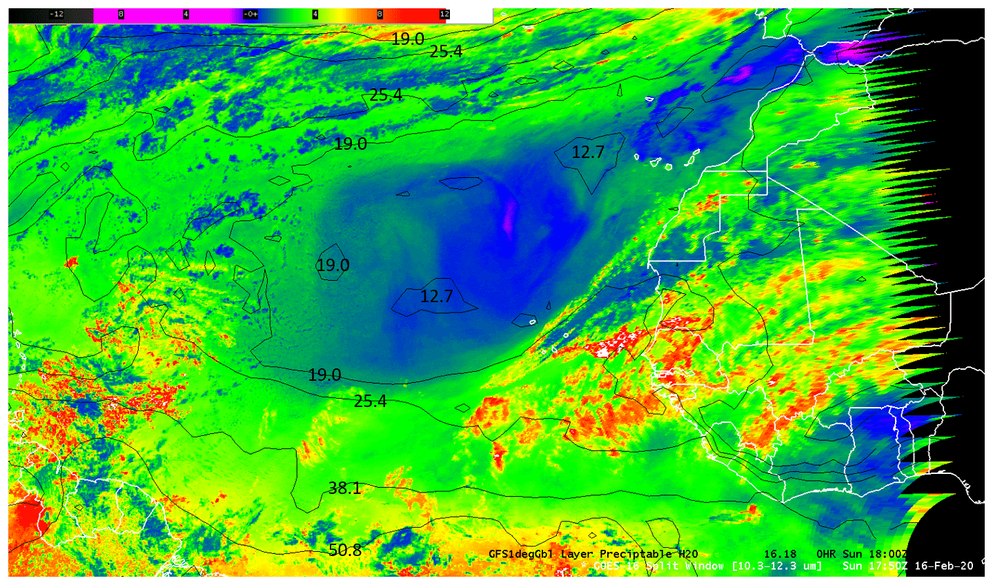
Figure 11The same as Fig. 10, except TPW (mm) is plotted on the GOES-16 ABI Tb(10.35 µm) − Tb(12.3 µm) channel difference (∘C).
One of the uses of microwave data is the retrieval of water vapor. As stated above, Forsythe et al. (2015) developed a methodology to retrieve values of water vapor in layers of the troposphere, referred to as the ALPW product. Due to the use of LEO sensors, imagery for the ALPW was not necessarily available as often as ABI data from GOES-16. Subsequently, retrieved values of ALPW, in the layer from the surface to 850 hPa, valid at 03:00 UTC 17 February 2020, are displayed in Fig. 12. Previously, this paper speculated that values of dew point temperature at the surface decreased from south to north, relative to the Tb maximum in Fig. 8. Values of the ALPW in Fig. 12 support the speculation; i.e., values of the ALPW decreased from the south, with values approximately 27.9 mm, to the north, with values near 15.4 mm.

Figure 12Advected Layer Precipitable Water product (mm) for the surface to 850 hPa layer, valid at 03:00 UTC 17 February 2020.
A second layer of values of the ALPW from 700 to 500 hPa is shown in Fig. 13. Two characteristics of values of the ALPW in the second layer were that (1) a relatively large region of the northern half of the image had values near 2.5 mm and that (2) values of the ALPW increased towards the south to values near 12.7 mm. Further, the boundary between dark grey and green was co-located with the southern edge of the region of largest values of Tb near 7.34 µm where values of GFS TPW increase from about 19 to near 25 mm (Fig. 8). Note also that the region of the NDR in the GeoColor image (Fig. 10) was co-located with the smallest values of ALPW in Figs. 12 and 13. In contrast, values of the ALPW in Figs. 12 and 13 increased in the SDR, particularly in Fig. 13. In addition, values of the channel difference displayed in the same scene as Figs. 12 and 13 also showed a dust signal (Fig. 14) that was also co-located with the smallest values of ALPW in the NDR in Figs. 12 and 13. In contrast, values of the channel difference increased to values near 3 to 4 ∘C in the SDR, similar to values of the channel difference 9 h earlier in Fig. 5.
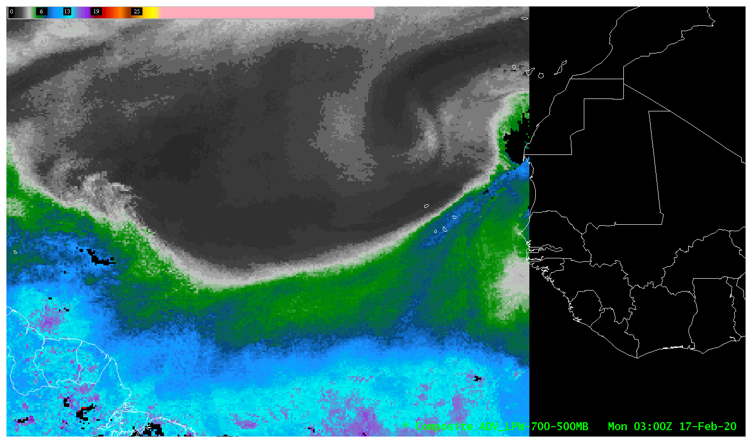
Figure 13The same as Fig. 12, except for the 700 to 500 hPa layer valid at 03:00 UTC 17 February 2020.
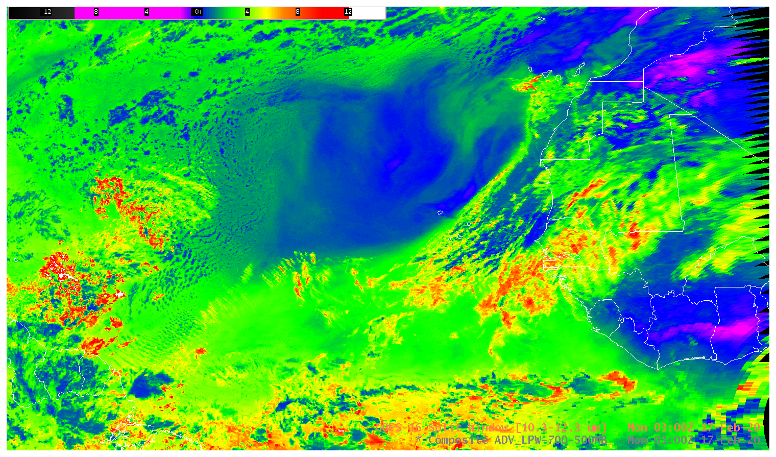
Figure 14GOES-16 ABI Tb(10.35 µm) − Tb(12.3 µm) channel difference (∘C) valid at 03:00 UTC 17 February 2020.
In addition to the retrieval of values of ALPW, data from NUCAPS were used to diagnose TPW. Because data from LEO satellites are used by the NUCAPS algorithm, gridded values of TPW are shown in Fig. 15, valid at 03:33 UTC 17 February 2020, which was the time of the granule shown in Fig. 15. A large region of values of TPW north of approximately 15∘ N, in the NDR, varied between 12 and 16 mm. In sharp contrast, values of TPW south of approximately 15∘N, in the SDR, increase over a relatively short distance to values in excess of 26 mm. In order to further examine the three-dimensional structure of the scene shown in Fig. 15, retrieved NUCAPS soundings were examined.
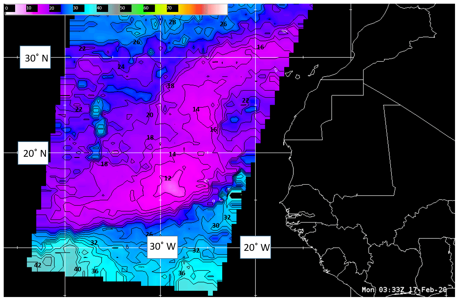
Figure 15Gridded NUCAPS TPW (mm) valid at 03:33 UTC 17 February 2020, which represents the time of the granule in the image.
A swath of locations of NUCAPS soundings is shown in Fig. 16. NUCAPS sounding locations, indicated by green dots, were superimposed on an ABI low-level water vapor image in order to relate soundings to the NDR and SDR. Both datasets were valid at 02:40 UTC 17 February 2020, which was the beginning time of the orbit. Nine soundings from NUCAPS in the NDR were examined, the location of a representative sounding site is bounded by a white circle and identified by the numeral 1 and will be referred to as Sounding-1. Similarly, three soundings from NUCAPS were examined in the SDR, a circle bounds the location of a representative sounding site, is denoted by the numeral 2, and will be referred to as Sounding-2. Because the horizontal areal extent of the NDR in Fig. 16 was larger than the horizontal extent of the SDR, more NUCAPS soundings were used to sample the NDR compared to the sample size of the SDR. Both NUCAPS-retrieved soundings, Sounding-1 and Sounding-2, are displayed in Fig. 17. A noticeable characteristic of Sounding-1 was the relatively large value of the difference between the temperature and the dew point temperature of several tens of degrees Celsius, especially in the layer between 700 and 500 hPa, which was coincident with the weighting function peak of the low-level water vapor image (Fig. 8). All of the other eight NUCAPS soundings in the NDR contained a similar difference between the temperature and dew point temperature. In contrast, however, values of the difference between the temperature and dew point temperature in Sounding-2 were on the order of 10 ∘C; a characteristic shared by the other NUCAPS soundings in the SDR. Observations suggested that the relatively low water vapor content characteristic of the NDR compared to the SDR allowed dust to be detected by the ABI Tb(10.35 µm) − Tb(12.3 µm) difference in the NDR compared to the SDR.
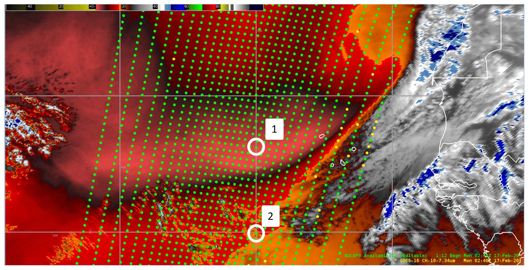
Figure 16Low-level water vapor image from GOES-16 ABI along with a swath of locations (dots) of NUCAPS soundings, both valid at 02:40 UTC 17 February 2020. Numerals 1 and 2 denote locations from which retrieved NUCAPS soundings were extracted.
There were important consequences of the relatively low water vapor content characteristic of the NDR compared to the SDR. First, the ABI Tb(10.35 µm) − Tb(12.3 µm) difference had values that were negative down to near zero, which was consistent with dust in the NDR. Thus, relatively low values of water vapor allowed dust to be detected. One counterargument against the use of the ABI infrared channel difference is that dust was evident in GeoColor images (Fig. 10). A close examination of Fig. 10, however, shows that the day–night terminator was near the western coast of Africa at 18:00 UTC 16 February 2020. Once solar reflection ceased over the eastern Atlantic Ocean, GeoColor imagery was unable to reveal future locations of dust in the NDR. Thus, a second consequence of relatively low water vapor content was that the dust field in the NDR may be tracked in time without solar reflection, which was demonstrated in a time sequence of nighttime images of values of the ABI Tb(10.35 µm) − Tb(12.3 µm) illustrated in Fig. 18. One feature was highlighted from 20:00 UTC 16 February 2020 to 02:00 UTC 17 February 2020 in Fig. 18: over the 6 h time period, the horizontal pattern of the channel difference exhibited little change, which supports the relatively slow temporal morphology of the dust contained in the discussion for Fig. 7a.
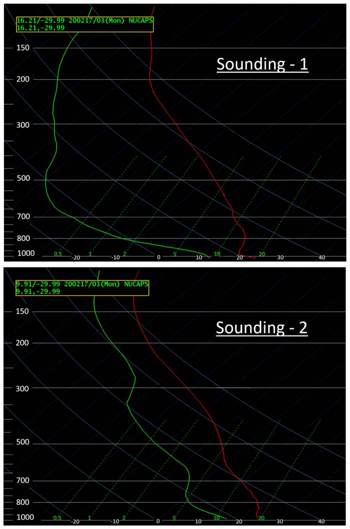
Figure 17Atmospheric soundings, denoted Sounding-1 and Sounding-2, from the location identified by the numerals 1 and 2 in Fig. 16. Sounding-1 illustrates the dry atmosphere that is characteristic of the northern dust region compared to an atmosphere that is more moist and is characteristic of the southern dust region.
As shown above, detection of dust in the SDR, by means of the infrared channel difference, was masked by water vapor. Undetected dust layers may hamper studies of both the direct radiative effect scattering of energy by dust particles and the indirect radiative effect microphysical impacts on cloud lifetimes. Further, undetected dust layers may pose a hazard to both civilian and military aviation through a reduction of visibility and potential damage to aircraft engines. Undetected dust presents a different significance and concern depending on the application. For example, hazard to aircraft may be deemed more significant and be of a higher level of concern compared to scattering of solar and longwave radiation by undetected dust layers. As discussed above, GeoColor imagery detected dust in the SDR. However, GeoColor imagery relied on measurements of reflected solar energy; as a result, dust will go undetected after sunset in the SDR. However, dust in the NDR was not only detected but also tracked after sunset. One potential method for nighttime detection of dust in the SDR may come from a future day–night band (DNB, Miller et al., 2013) on a geostationary satellite. Nighttime dust and smoke detection may be afforded by a DNB through the measurement of reflected moonlight.
There have been increasing research efforts to assimilate dust (or aerosol in general) into numerical models for the improvement of aerosol weather forecasts over the last 2 decades (Collins et al., 2001; Wang et al., 2003; Weaver et al., 2007; Wang and Niu, 2013; Zhang et al., 2014; Lee et al., 2017). In addition to research efforts, many operational numerical weather prediction (NWP) centers have included aerosols in their assimilation systems to provide routine aerosol forecast and aerosol reanalysis (Xian et al., 2019). The following is a brief list of some NWP centers and their efforts: the US Navy Fleet Numerical Meteorology and Oceanography Center (FNMOC), which employs the Navy Aerosol Analysis and Prediction System (NAAPS) to provide reanalysis (Lynch et al., 2016) and ensemble forecast (Rubin et al., 2017) of aerosol distribution; the European Centre for Medium-Range Weather Forecasts (ECMWF), which utilizes a 4D-Var data assimilation algorithm to update aerosol and atmospheric states in their Integrated Forecast System (IFS) (Morcrette et al., 2008; Benedetti et al., 2009); and the Japan Meteorological Agency (JMA), which runs the Model of Aerosol Species in the Global Atmosphere (MASINGAR; Tanaka and Chiba, 2005), as well as a 2D-Var data assimilation method to provide operational aerosol and dust forecasts and analyses (Yumimoto et al., 2018). In addition, the NASA Global Modeling and Assimilation Office (GMAO) also assimilates aerosols in their Goddard Earth Observing System Version 5 (GEOS-5; Randles et al., 2017).

Figure 18Time series of the GOES-16 ABI Tb(10.35 µm) − Tb(12.3 µm) channel difference (∘C) highlighting the morphology of dust over a 7.5 h time period. In addition, the time series demonstrates that the dust could be tracked at night.
Currently, the NOAA National Centers for Environmental Prediction (NCEP) employs the NOAA Environmental Modeling System (NEMS) Global Forecast System (GFS) Aerosol Component (NGAC) for global dust forecasting (Lu et al., 2016a). Development of NGAC is a collaborative ongoing effort between NCEP and NASA toward aerosol data assimilation capability in NCEP. Currently, there are plans to implement the aerosol assimilation capabilities in Gridpoint Statistical Interpolation (GSI; Pagowski et al., 2014) and the Community Radiative Transfer Model (CRTM; Han et al., 2007) into NGAC to allow the direct assimilation of satellite radiances affected by aerosol and assimilation of aerosol optical depth (Lu et al., 2016b). Using this information, the simple channel difference discussed in this paper can be used to aid operational forecast of dust via data assimilation.
SAL airborne dust plumes can be transported across the Atlantic Ocean along the southern periphery of a North Atlantic subtropical high pressure system toward southern Florida. Transport of the SAL may be enhanced when a subtropical high-pressure system becomes zonally elongated towards southern portions of the United States, allowing for more direct westward transport of the SAL towards southern Florida. Thus, both detection and tracking of the SAL is important for the preparation against potential impacts on southern Florida.
As mentioned above, due to the scarcity of both in situ surface and upper-air observations, spaceborne instruments are essential across the tropical and subtropical Atlantic, Caribbean, and Gulf of Mexico basins. An important benefit of having a spaceborne sensor observe the SAL is the tendency of the SAL to transition from a relatively large homogeneous air mass near Africa to an increasingly fractured, irregularly shaped dust plume during its westward migration across the Atlantic basin. In addition, the appearance of the SAL may also change due to encounters with dust-scavenging rain systems of varying scale. Accurate and timely observations of smaller, irregularly shaped dust plumes via products derived from both geostationary and polar-orbiting satellites are essential for anticipating important changes in lapse rates and convective instability. Accurately discerning the horizontal and vertical extent of the SAL can aid the prediction of severe weather potential. Thus, National Weather Service (NWS) meteorologists of southern Florida benefit greatly from tracking the SAL, as it can be a proxy for the movement and evolution of an elevated mixed layer (EML; Carlson and Ludlam, 1968; Lanicci and Warner, 1991). EMLs may lead to a dramatic increase in convective available potential energy, especially when the SAL surmounts a maritime tropical air mass with high values of moist static energy near the Florida peninsula.
Although the SAL has been known to influence local weather, the SAL also has the ability to impact both air quality and visibility. Airborne dust can affect the health and safety of the public, either via direct respiratory impacts or indirectly via reductions in horizontal surface visibility (Kuciauskas et al., 2018). In particular, decreases in the line-of-sight visibility have a direct impact on aviation. Furthermore, awareness of the SAL directly enhances the impact decision support service (IDSS); IDSS is provided to core partners who rely on the NWS for timely and accurate severe weather threat assessments in order to protect life and property.
This paper examined satellite observations of a dust plume associated with the SAL that moved from western Africa westward over the eastern Atlantic Ocean. Observations from several sensors aboard satellite platforms were used herein: ABI onboard GOES-16, VIIRS onboard NOAA-20, and CALIOP onboard CALIPSO. Further, the quantification of vertically integrated water vapor was retrieved from two remote sources, each of which used multiple sensors from multiple satellites: NUCAPS and MIRS. Satellite observations of the dust plume associated with the SAL presented herein extended from 16 to 17 February 2020. Examination of the dust plume associated with the SAL employed GeoColor, low-level water vapor, and split window difference imagery from GOES-16 ABI; True-Color and split window difference imagery from VIIRS; VFM from CALIOP; gridded TPW and retrieved skew-T data from NUCAPS; and the ALPW product from MIRS. Observational data from all of the aforementioned satellite platforms were used for the purpose of extending and supporting two previous numerical studies, which hypothesized that water vapor may mask infrared detection of dust.
Numerical studies have been used to examine the impact of water vapor on dust detection. Both Miller et al. (2019) and Banks et al. (2019) used numerical methods to show that when vertically integrated water vapor increased above some value, dust may be masked by water vapor; thus, making dust detection with simulated or synthetic infrared imagery a challenge. Satellite observations of the African dust plume from 16–17 February 2020 provided observational support for the two numerical studies stated above. Specifically, GeoColor imagery from ABI, True-Color imagery from VIIRS, and the VFM from CALIOP all revealed the existence of dust in both the NDR and SDR. However, both the Tb(10.35 µm) − Tb(12.30 µm) split window difference from ABI and the EUMETSAT infrared dust product suggested the existence of dust only in the NDR. Values of integrated water vapor exhibited a noticeable difference between the NDR and the SDR.
Data from MIRS and NUCAPS can be summarized as follows. Specifically, the 03:00 UTC 17 February 2020 values of the ALPW product in the surface to 850 hPa layer decreased from the SDR, with values approximately 27.9 mm, to the NDR, with values near 15.4 mm, an approximate 44 % decrease (Fig. 12). Further, values of the ALPW product in the 700 to 500 hPa layer decreased from the SDR, with values near 12.7 mm, to the NDR, with values near 2.5 mm, an approximate 80 % decrease (Fig. 13). In addition, the 03:33 UTC 17 February 2020 values of gridded TPW decreased from the SDR, with values near 26 mm, to the NDR, with values near 12 to 16 mm, an approximate 38 % decrease (Fig. 15). In both cases a distinct horizontal gradient of values of both the ALPW product from MIRS and gridded TPW from NUCAPS existed near 15∘ N, the approximate boundary between the SDR and NDR. Furthermore, the location of the distinct horizontal gradient of values of both the ALPW product and TPW were approximately co-located with a distinct horizontal gradient of values of the Tb(10.35 µm) − Tb(12.30 µm) split window difference from ABI (Fig. 5) and the southern boundary of the dust signal in the EUMETSAT dust product (Fig. 6). Thus, observations show that dust within the SDR and NDR was masked and detected where values of both ALPW and gridded TPW were the largest (sfc-805 hPa ALPW ∼27.9 mm, TPW ∼26 mm) and smallest (sfc-850 hPa ALPW ∼15.4 mm, TPW ∼14 mm). Furthermore, representative vertical sounding from NUCAPS exhibited a distinctly drier atmosphere in the NDR compared to the SDR (Fig. 17). Consequently, satellite imagery and products of 16–17 February 2020 of an African dust plume lend observational support to the numerical results of both Miller et al. (2019) and Banks et al. (2019).
An important consequence of the observational study in this paper is relevant to NWS forecasters. There are two aspects of the SAL that are important to NWS forecasters: (1) dust in the SAL and (2) the associated EML within the SAL. Dust within the SAL may impact not only respiratory function in people but also aviation operations. An associated EML within the SAL may lead to the development of severe thunderstorms. As a result, the detection and tracing of dust layers from Africa is important to NWS forecasters. Assimilation of dust into operational forecast models may help improve the forecasting of not only dust itself but also the thermodynamic profile of an associated EML with the SAL.
AWIPS-2 code is protected by license and unavailable.
Satellite data are available via the CLASS site. Because CIRA is not a satellite data repository, satellite data are available from NOAA'S Comprehensive Large Array-data Stewardship System at https://www.class.noaa.gov (last access: 15 March 2020, NOAA, 2020).
LG and DB conceived the study of this paper. LG prepared the manuscript with the help of all co-authors. JT, JFD, and HQC provided support for the acquisition of satellite data. JF and EB provided support with retrievals from MIRS and NUCAPS. TCW contributed data assimilation expertise. Both HGW and KBK served as NWS collaborators, and SDM provided support for results from the MURI.
The authors declare that they have no conflict of interest.
The authors gratefully acknowledge that this research was primarily funded by the NOAA GOES-R Program Office (NA19OAR4320073) and the DOD/ONR/MURI (N00014-16-1-2040). The views, opinions, and findings in this report are those of the authors and should not be construed as an official NOAA and or U.S. Government position, policy, or decision.
This research has been supported by the NOAA GOES-R Program Office (grant no. NA19OAR4320073) and the DOD/ONR/MURI (grant no. N00014-16-1-2040).
This paper was edited by Edward Nowottnick and reviewed by two anonymous referees.
Ackerman, S. A.: Using the radiative temperature difference at 3.7 and 11 µm to tract dust outbreaks, Remote Sens. Environ., 27, 129–133, https://doi.org/10.1016/0034-4257(89)90012-6, 1989.
Ackerman, S. A.: Remote sensing aerosols using satellite infrared observations, J. Geophys. Res.-Atmos., 102, 17069–17079, https://doi.org/10.1029/96jd03066, 1997.
Adams, A. M., Prospero, J. M., and Zhang, C.: CALIPSO-Derived three-dimensional structure of aerosol over the atlantic basin and adjacent continents, J. Climate, 25, 6862–6879, https://doi.org/10.1175/JCLI-D-11-00672.1, 2012.
Ahmadov, R., Grell, G., James, E., Csiszar, I., Tsidulko, M., Pierce, B., McKeen, S., Benjamin, S., Alexander, C., Pereira, G., Freitas, S., and Goldberg, M.: Using VIIRS Fire Radiative Power data to simulate biomass burning emissions, plume rise and smoke transport in a real-time air quality modeling system, in: Int. Geosci. Remote Se., Fort Worth, TX, 23–28 July 2017, 2806–2808, 2017.
Ashpole, I. and Washington, R.: An automated dust detection using SEVIRI: A multiyear climatology of summertime dustiness in the central and western Sahara, J. Geophys. Res., 117, D08202, https://doi.org/10.1029/2011JD016845, 2012.
Banks, J. R., Hünerbein, A., Heinold, B., Brindley, H. E., Deneke, H., and Schepanski, K.: The sensitivity of the colour of dust in MSG-SEVIRI Desert Dust infrared composite imagery to surface and atmospheric conditions, Atmos. Chem. Phys., 19, 6893–6911, https://doi.org/10.5194/acp-19-6893-2019, 2019.
Benedetti, A., Morcrette, J. J., Boucher, O., Dethof, A., Engelen, R. J., Fisher, M., Flentje, H., Huneeus, N., Jones, L., Kaiser, J. W., Kinne, S., Mangold, A., Razinger, M., Simmons, A. J., and Suttie, M.: Aerosol analysis and forecast in the European Centre for Medium-Range Weather Forecasts integrated forecast system: 2. data assimilation, J. Geophys. Res., 114, D13205, https://doi.org/10.1029/2008JD011115, 2009.
Berndt, E. and Folmer, M.: Utility of CrIS/ATMS profiles to diagnose extratropical transition, Results Phys., 8, 184–185, https://doi.org/10.1016/j.rinp.2017.12.006, 2018.
Berndt, E., Elmer, N., Schultz, L., and Molthan, A.: A Methodology to Determine Recipe Adjustments for Multispectral Composites Derived from Next-Generation Advanced Satellite Imagers, J. Atmos. Ocean. Tech., 35, 643–664, 2018.
Berndt, E. B., Zavodsky, B. T., and Folmer, M. J.: Development and Application of Atmospheric Infrared Sounder Ozone Retrieval Products for Operational Meteorology, IEEE T. Geosci. Remote, 54, 958–967, https://doi.org/10.1109/TGRS.2015.2471259, 2016.
Berndt, E. B., White, K. D., Smith, N., and Esmaili, R.: Operational Transition of Gridded NUCAPS to NOAA NWS and Emerging Applications, in AMS 16th Annual Symposium on New Generation Operational Enviornmental Satellite Systems, Boston, MA, 13 January 2020, available at: https://ams.confex.com/ams/2020Annual/meetingapp.cgi/Paper/367631, last access: 28 April 2020.
Bloch, C., Knuteson, R. O., Gambacorta, A., Nalli, N. R., Gartzke, J., and Zhou, L.: Near-Real-Time Surface-Based CAPE from Merged Hyperspectral IR Satellite Sounder and Surface Meteorological Station Data, J. Appl. Meteorol. Climatol., 58, 1613–1632, https://doi.org/10.1175/JAMC-D-18-0155.1, 2019.
Boukabara, S. A., Garrett, K., Chen, W., Iturbide-Sanchez, F., Grassotti, C., Kongoli, C., Chen, R., Liu, Q., Yan, B., Weng, F., Ferraro, R., Kleespies, T. J., and Meng, H.: MiRS: An all-weather 1DVAR satellite data assimilation and retrieval system, IEEE T. Geosci. Remote, 49, 3249–3272, https://doi.org/10.1109/TGRS.2011.2158438, 2011.
Carlson, T. N. and Ludlam, F. H.: Conditions for the occurrence of severe local storms, Tellus A, 20, 203–226, https://doi.org/10.3402/tellusa.v20i2.10002, 1968.
Chaboureau, J. P., Tulet, P., and Mari, C.: Diurnal cycle of dust and cirrus over West Africa as seen from Meteosat Second Generation satellite and a regional forecast model, Geophys. Res. Lett., 34, 2–6, https://doi.org/10.1029/2006GL027771, 2007.
Cho, H. M., Nasiri, S. L., Yang, P., Laszlo, I., and Zhao, X. T.: Detection of optically thin mineral dust aerosol layers over the ocean using MODIS, J. Atmos. Ocean. Tech., 30, 896–916, https://doi.org/10.1175/JTECH-D-12-00079.1, 2013.
Collins, W. D., Rasch, P. J., Eaton, B. E., Khattatov, B. V., Lamarque, J. F., and Zender, C. S.: Simulating aerosols using a chemical transport model with assimilation of satellite aerosol retrievals: Methodology for INDOEX, J. Geophys. Res.-Atmos., 106, 7313–7336, https://doi.org/10.1029/2000JD900507, 2001.
Csiszar, I., Schroeder, W., Giglio, L., Ellicott, E., Vadrevu, K. P., Justice, C. O., and Wind, B.: Active fires from the Suomi NPP Visible Infrared Imaging Radiometer Suite: Product status and first evaluation results Ivan, J. Geophys. Res.-Atmos., 119, 803–816, https://doi.org/10.1002/2013JD020453, 2014.
Darmenov, A. and Sokolik, I. N.: Identifying the regional thermal-IR radiative signature of mineral dust with MODIS, Geophys. Res. Lett., 32, L16803, https://doi.org/10.1029/2005GL023092, 2005.
Dunion, J. P. and Velden, C. S.: The Impact of the Saharan Air Layer on Atlantic Tropical Cyclone Activity, B. Am. Meteorol. Soc., 85, 353–365, https://doi.org/10.1175/BAMS-85-3-353, 2004.
Esmaili, R. B., Smith, N., Berndt, E. B., Dostalek, J. F., Kahn, B. H., White, K., Barnet, C. D., Sjoberg, W., and Goldberg, M.: Adapting satellite soundings for operational forecasting within the hazardous weather testbed, Remote Sens., 12, 886, https://doi.org/10.3390/rs12050886, 2020.
Forsythe, J. M., Kidder, S. Q., Fuell, K. K., Leroy, A., Jedlovec, G. J., and Jones, A. S.: A Multisensor, Blended, Layered Water Vapor Product for Weather Analysis and Forecasting, J. Oper. Meteorol., 3, 41–58, 2015.
Gambacorta, A.: The NOAA Unique CrIS/ATMS Processing System (NUCAPS): Algorithm Theoretical Basis Documentation, Version 1.0, NOAA, available at: https://www.ospo.noaa.gov/Products/atmosphere/soundings/nucaps/docs/NUCAPS_ATBD_20130821.pdf (last access: 16 February 2021), 2013.
Gambacorta, A. and Barnet, C. D.: Methodology and information content of the NOAA NESDIS operational channel selection for the cross-track infrared sounder (CrIS), IEEE T. Geosci. Remote, 51, 3207–3216, https://doi.org/10.1109/TGRS.2012.2220369, 2013.
Gitro, C. M., Jurewicz, Sr., M. L., Kusselson, S. J., Forsythe, J. M., Kidder, S. Q., Szoke, E. J., Bikos, D., Jones, A. S., Gravelle, C. M., and Grassotti, C.: Using the Multisensor Advected Layered Precipitable Water Product in the Operational Forecast Environment, J. Oper. Meteorol., 06, 59–73, https://doi.org/10.15191/nwajom.2018.0606, 2018.
Goldberg, M. D., Kilcoyne, H., Cikanek, H., and Mehta, A.: Joint Polar Satellite System: The United States next generation civilian polar-orbiting environmental satellite system, J. Geophys. Res.-Atmos., 118, 13463–13475, https://doi.org/10.1002/2013JD020389, 2013.
Goodman, S., Schmit, T., Daniels, J., and Redmon, R.: The GOES-R Series: A New Generation of Geostationary Environmental Satellites, 1st edn., Elsevier, Amsterdam, Netherlands, Oxford, United Kingdom, Cambridge, United States, 2019.
Goodman, S. J., Gurka, J., De Maria, M., Schmit, T. J., Mostek, A., Jedlovec, G., Siewert, C., Feltz, W., Gerth, J., Brummer, R., Miller, S., Reed, B., and Reynolds, R. R.: The goes-R proving ground: Accelerating user readiness for the next-generation geostationary environmental satellite system, B. Am. Meteorol. Soc., 93, 1029–1040, https://doi.org/10.1175/BAMS-D-11-00175.1, 2012.
Han, Y., Weng, F., P., Liu, and van Delst, P.: A fast radiative transfer model for SSMIS upper atmospheric sounding channels, J. Geophys. Res.-Atmos., 112, D11121, https://doi.org/1029/2006JD008208, 2007.
Hao, X. and Qu, J. J.: Saharan dust storm detection using moderate resolution imaging spectroradiometer thermal infrared bands, J. Appl. Remote Sens., 1, 013510, https://doi.org/10.1117/1.2740039, 2007.
Heidinger, A. K., Li, Y., Baum, B. A., Holz, R. E., Platnick, S., and Yang, P.: Retrieval of cirrus cloud optical depth under day and night conditions from MODIS Collection 6 cloud property data, Remote Sens., 7, 7257–7271, https://doi.org/10.3390/rs70607257, 2015.
Herman, J. R., Bhartia, P. K., Torres, O., Hsu, C., Seftor, C., and Celarier, E.: Global distribution of UV-absorbing aerosols from Nimbus 7/TOMS data, J. Geophys. Res.-Atmos., 102, 16911–16922, https://doi.org/10.1029/96jd03680, 1997.
Hillger, D. and Ellrod G. P.: Detection of important atmospheric and surface features by employing principal component image transformation of GOES imagery, J. Appl. Meteorol. Climatol., 42, 611–629, https://doi.org/10.1175/1520-0450(2003)042<0611:DOIAAS>2.0.CO;2, 2003.
Hillger, D., Kopp, T., Lee, T., Lindsey, D., Seaman, C., Miller, S., Solbrig, J., Kidder, S., Bachmeier, S., Jasmin, T., and Rink, T.: First-light imagery from Suomi NPP VIIRS, B. Am. Meteorol. Soc., 94, 1019–1029, https://doi.org/10.1175/BAMS-D-12-00097.1, 2013.
Hillger, D., Seaman, C., Liang, C., Miller, S., Lindsey, D., and Kopp, T.: Suomi NPP VIIRS Imagery evaluation, J. Geophys. Res., 119, 6440–6455, https://doi.org/10.1002/2013JD021170, 2014.
Holton, J. R.: An Introduction to Dynamic Meteorology, Academic Press, New York, 1979.
Hunt, W. H., Vaughan, M. A., Powell, K. A., and Weimer, C.: CALIPSO lidar description and performance assessment, J. Atmos. Ocean. Tech., 26, 1214–1228, https://doi.org/10.1175/2009JTECHA1223.1, 2009.
Iturbide-Sanchez, F., Da Silva, S. R. S., Liu, Q., Pryor, K. L., Pettey, M. E., and Nalli, N. R.: Toward the operational weather forecasting application of atmospheric stability products derived from NUCAPS CrIS/ATMS Soundings, IEEE T. Geosci. Remote, 56, 4522–4545, https://doi.org/10.1109/TGRS.2018.2824829, 2018.
Kalluri, S., Alcala, C., Carr, J., Griffith, P., Lebair, W., Lindsey, D., Race, R., Wu, X., and Zierk, S.: From photons to pixels: Processing data from the Advanced Baseline Imager, Remote Sens., 10, 177, https://doi.org/10.3390/rs10020177, 2018.
King, M. D., Kaufman, Y. J., Menzel, W. P., and Tanre, D.: Remote sensing of cloud, aerosol, and water vapor properties from the moderate resolution imaging spectrometer (MODIS), IEEE T. Geosci. Remote, 30, 2–27, https://doi.org/10.1109/36.124212, 1992.
Knippertz, P. and Todd, M. C.: The central west Saharan dust hot spot and its relation to African easterly waves and extratropical disturbances, J. Geophys. Res.-Atmos., 115, 1–14, https://doi.org/10.1029/2009JD012819, 2010.
Kuciauskas, A. P., Xian, P., Hyer, E. J., Oyola, M. I., and Campbell, J. R.: Supporting weather forecasters in predicting and monitoring Saharan air layer dust events as they impact the greater Caribbean, B. Am. Meteorol. Soc., 99, 259–268, https://doi.org/10.1175/BAMS-D-16-0212.1, 2018.
Lanicci, J. M. and Warner, T. T.: A Synoptic Climatology of the Elevated Mixed-Layer Inversion over the Southern Great Plains in Spring. Part III: Relationship to Severe-Storms Climatology, Weather Forecast., 6, 214–226 1991.
Lee, E., Županski, M., Županski, D., and Park, S. K.: Impact of the OMI aerosol optical depth on analysis increments through coupled meteorology–aerosol data assimilation for an Asian dust storm, Remote Sens. Environ., 193, 38–53, https://doi.org/10.1016/j.rse.2017.02.013, 2017.
Legrand, M., Berthand, J. J., Desbois, M., Menenger, L., and Fouquart, Y.: The Potential of Infrared Satellite Data for the Retrieval of Saharan-Dust Optical Depth over Africa, J. Appl. Meteorol., 28, 309–318, https://doi.org/10.1175/1520-0450(1989)028<0309:TPOISD>2.0.CO;2, 1989.
Legrand, M., Plana-Fattori, A., and N'Doumé, C.: Satellite detection of dust using the IR imagery of Meteosat 1. Infrared difference dust index, J. Geophys. Res.-Atmos., 106, 18251–18274, https://doi.org/10.1029/2000JD900749, 2001.
Lensky, I. M. and Rosenfeld, D.: Clouds-Aerosols-Precipitation Satellite Analysis Tool (CAPSAT), Atmos. Chem. Phys., 8, 6739–6753, https://doi.org/10.5194/acp-8-6739-2008, 2008.
LeRoy, A., Fuell, K., Molthan, A., Jedlovec, G., Forsythe, J., Kidder, S., and Jones, A.: The operational use and assessment of a layered precipitable water product for weather forecasting, J. Oper. Meteorol., 4, 22–33, https://doi.org/10.15191/nwajom.2016.0402, 2016.
Liu, Z., Omar, A. H., Hu, Y., Vaughan, M. A., and Winker, D. M.: CALIOP Algorithm Theoretical Basis Document. Part 3: Scene classification algorithms, 1–56, available at: https://www-calipso.larc.nasa.gov/resources/pdfs/PC-SCI-202_Part3_v1.0.pdf (last access: 10 February 2021), 2005.
Lu, C.-H., da Silva, A., Wang, J., Moorthi, S., Chin, M., Colarco, P., Tang, Y., Bhattacharjee, P. S., Chen, S.-P., Chuang, H.-Y., Juang, H.-M. H., McQueen, J., and Iredell, M.: The implementation of NEMS GFS Aerosol Component (NGAC) Version 1.0 for global dust forecasting at NOAA/NCEP, Geosci. Model Dev., 9, 1905–1919, https://doi.org/10.5194/gmd-9-1905-2016, 2016.
Lu, S., Wei, S., Kondragunta, S., Zhao, Q., Mcqueen, J., Wang, J., and Bhattacharjee, P.: NCEP Aerosol Data Assimilation Update: Improving NCEP global aerosol forecasts using JPSS-NPP VIIRS aerosol products, in: ICAP Working Group Meeting, College Park, MD, 1–31, 2016b.
Lynch, P., Reid, J. S., Westphal, D. L., Zhang, J., Hogan, T. F., Hyer, E. J., Curtis, C. A., Hegg, D. A., Shi, Y., Campbell, J. R., Rubin, J. I., Sessions, W. R., Turk, F. J., and Walker, A. L.: An 11-year global gridded aerosol optical thickness reanalysis (v1.0) for atmospheric and climate sciences, Geosci. Model Dev., 9, 1489–1522, https://doi.org/10.5194/gmd-9-1489-2016, 2016.
Miller, S. D.: A consolidated technique for enhancing desert dust storms with MODIS, Geophys. Res. Lett., 30, 2071, https://doi.org/10.1029/2003GL018279, 2003.
Miller, S. D., Mills, S. P., Elvidge, C. D., Lindsey, D. T., Lee, T. F., and Hawkins, J. D.: Suomi satellite brings to light a unique frontier of nighttime environmental sensing capabilities, P. Natl. Acad. Sci. USA, 109, 15706–15711, https://doi.org/10.1073/pnas.1207034109, 2012.
Miller, S. D., Straka, W., Mills, S. P., Elvidge, C. D., Lee, T. F., Solbrig, J., Walther, A., Heidinger, A. K., and Weiss, S. C.: Illuminating the capabilities of the suomi national Polar-orbiting partnership (NPP) visible infrared imaging radiometer suite (VIIRS) day/night Band, Remote Sens., 5, 6717–6766, https://doi.org/10.3390/rs5126717, 2013.
Miller, S. D., Schmit, T. L., Seaman, C. J., Lindsey, D. T., Gunshor, M. M., Kohrs, R. A., Sumida, Y., and Hillger, D.: A sight for sore eyes: The return of true color to geostationary satellites, B. Am. Meteorol. Soc., 97, 1803–1816, https://doi.org/10.1175/BAMS-D-15-00154.1, 2016.
Miller, S. D., Bankert, R. L., Solbrig, J. E., Forsythe, J. M., Noh, Y.-J., and Grasso, L. D.: A Dynamic Enhancement With Background Reduction Algorithm: Overview and Application to Satellite-Based Dust Storm Detection, J. Geophys. Res.-Atmos., 122, 938–959, https://doi.org/10.1002/2017JD027365, 2017.
Miller, S. D., Grasso, L. D., Bian, Q., Kreidenweis, S. M., Dostalek, J. F., Solbrig, J. E., Bukowski, J., van den Heever, S. C., Wang, Y., Xu, X., Wang, J., Walker, A. L., Wu, T.-C., Zupanski, M., Chiu, C., and Reid, J. S.: A Tale of Two Dust Storms: analysis of a complex dust event in the Middle East, Atmos. Meas. Tech., 12, 5101–5118, https://doi.org/10.5194/amt-12-5101-2019, 2019.
Miller, S. D., Lindsey, D. T., Seaman, C. J., and Solbrig, J. E.: Geocolor: A blending technique for satellite imagery, J. Atmos. Ocean. Tech., 37, 429–448, https://doi.org/10.1175/JTECH-D-19-0134.1, 2020.
Morcrette, J. J., Beljaars, A., Benedetti, A., Jones, L., and Boucher, O.: Sea-salt and dust aerosols in the ECMWF IFS model, Geophys. Res. Lett., 35, L24813, https://doi.org/10.1029/2008GL036041, 2008.
Nalli, N. R., Barnet, C. D., Reale, T., Liu, Q., Morris, V. R., Spackman, J. R., Joseph, E., Tan, C., Sun, B., Tilley, F., Ruby Leung, L., and Wolfe, D.: Satellite sounder observations of contrasting tropospheric moisture transport regimes: Saharan air layers, hadley cells, and atmospheric rivers, J. Hydrometeorol., 17, 2997–3006, https://doi.org/10.1175/JHM-D-16-0163.1, 2016.
NOAA: Comprehensive Large Array-data Stewardship System (CLASS), available at: https://www.class.noaa.gov, last access: 15 March 2020.
Pagowski, M., Liu, Z., Grell, G. A., Hu, M., Lin, H.-C., and Schwartz, C. S.: Implementation of aerosol assimilation in Gridpoint Statistical Interpolation (v. 3.2) and WRF-Chem (v. 3.4.1), Geosci. Model Dev., 7, 1621–1627, https://doi.org/10.5194/gmd-7-1621-2014, 2014.
Pierangelo, C., Chédin, A., Heilliette, S., Jacquinet-Husson, N., and Armante, R.: Dust altitude and infrared optical depth from AIRS, Atmos. Chem. Phys., 4, 1813–1822, https://doi.org/10.5194/acp-4-1813-2004, 2004.
Prospero, J. M. and Carlson, T. N.: Vertical and areal distribution of Saharan dust over the western equatorial north Atlantic Ocean, J. Geophys. Res., 77, 5255–5265, https://doi.org/10.1029/JC077i027p05255, 1972.
Randles, C. A., da Silva, A. M., Buchard, V., Colarco, P. R., Darmenov, A., Govindaraju, R., Smirnov, A., Holben, B., Ferrare, R., Hair, J., Shinozuka, Y., and Flynn, C. J.: The MERRA-2 aerosol reanalysis, 1980 onward. Part I: Description and Data assimilation Evaluation, J. Climate, 30, 6823–6850, https://doi.org/10.1175/JCLI-D-16-0609.1, 2017.
Rubin, J. I., Reid, J. S., Hansen, J. A., Anderson, J. L., Holben, B. N., Xian, P., Westphal, D. L., and Zhang, J.: Assimilation of AERONET and MODIS AOT observations using variational and ensemble data assimilation methods and its impact on aerosol forecasting skill, J. Geophys. Res., 122, 4967–4992, https://doi.org/10.1002/2016JD026067, 2017.
Schlueter, A., Fink, A. H., and Knippertz, P.: A systematic comparison of tropical waves over Northern Africa. Part II: Dynamics and thermodynamics, J. Climate, 32, 2605–2625, https://doi.org/10.1175/JCLI-D-18-0651.1, 2019.
Schmetz, J., Pili, P., Tjemkes, S., Just, D., Kerkmann, J., Rota, S. and Ratier, A.: An Introduction to Meteosat Second Generation (MSG), B. Am. Meteorol. Soc., 83, 977–992, https://doi.org/10.1175/1520-0477(2002)083<0977:AITMSG>2.3.CO;2, 2002.
Schmit, T. J., Li, J., Gurka, J. J., Goldberg, M. D., Schrab, K. J., Li, J., and Feltz, W. F.: The GOES-R advanced baseline imager and the continuation of current sounder products, J. Appl. Meteorol. Climatol., 47, 2696–2711, https://doi.org/10.1175/2008JAMC1858.1, 2008.
Schmit, T. J., Griffith, P., Gunshor, M. M., Daniels, J. M., Goodman, S. J., and Lebair, W. J.: A closer look at the ABI on the goes-r series, B. Am. Meteorol. Soc., 98, 681–698, https://doi.org/10.1175/BAMS-D-15-00230.1, 2017.
Schmit, T. J., Lindstrom, S. S., Gerth, J. J., and Gunshor, M. M.: Applications of the 16 spectral bands on the Advanced Baseline Imager (ABI)., J. Oper. Meteorol., 06(04), 33–46, https://doi.org/10.15191/nwajom.2018.0604, 2018.
Shenk, W. E. and Curran, R. J.: The Detection of Dust Storms Over Land and Water With Satellite Visible and Infrared Measurements, Mon. Weather Rev., 102, 830–837, https://doi.org/10.1175/1520-0493(1974)102<0830:tdodso>2.0.co;2, 1974.
Shimizu, A.: Introduction of JMA VLab Support Site on RGB Composite Imagery and tentative RGBs, The 6th Asia/Oceania Meteorological Satellite Users' Conference, Tokyo, Japan, 9–13 November 2015, available at: http://www.data.jma.go.jp/mscweb/en/aomsuc6_data/presentations.html (last access: 10 February 2021), 2015.
Tanaka, T. Y. and Chiba, M.: Global simulation of dust aerosol with a chemical transport model, MASINGAR, J. Meteorol. Soc. Jpn., 83, 255–278, https://doi.org/10.2151/jmsj.83a.255, 2005.
Tanre, D. and Legrand, M.: On the satellite retrieval of Saharan dust optical thickness over land: two different approaches, J. Geophys. Res., 96, 5221–5227, https://doi.org/10.1029/90JD02607, 1991.
Torres, O., Bhartia, P. K., Herman, J. R., Ahmad, Z., and Gleason, J.: Derivation of aerosol properties from satellite measurements of backscattered ultraviolet radiation: Theoretical basis, J. Geophys. Res.-Atmos., 103, 17099–17110, https://doi.org/10.1029/98JD02709, 1998.
Torres, O., Tanskanen, A., Veihelmann, B., Ahn, C., Braak, R., Bhartia, P. K., Veefkind, P., and Levelt, P.: Aerosols and surface UV products form Ozone Monitoring Instrument observations: An overview, J. Geophys. Res.-Atmos., 112, D24S47, https://doi.org/10.1029/2007JD008809, 2007.
Wang, H. and Niu, T.: Sensitivity studies of aerosol data assimilation and direct radiative feedbacks in modeling dust aerosols, Atmos. Environ., 64, 208–218, https://doi.org/10.1016/j.atmosenv.2012.09.066, 2013.
Wang, J., Christopher, S. A., Brechtel, F., Kim, J., Schmid, B., Redemann, J., Russell, P. B., Quinn, P., and Holben, B. N.: Geostationary satellite retrievals of aerosol optical thickness during ACE-Asia, J. Geophys. Res., 108, 8657, https://doi.org/10.1029/2003JD003580, 2003.
Weaver, C., da Silva, A., Chin, M., Ginoux, P., Dubovik, O., Flittner, D., Zia, A., Remer, L., Holben, B., and Gregg, W.: Direct Insertion of MODIS Radiances in a Global Aerosol Transport Model, J. Atmos. Sci., 64, 808–827, https://doi.org/10.1175/JAS3838.1, 2007.
Weaver, G. M., Smith, N., Berndt, E. B., While, K. D., Dostalek, J. F., and Zavodsky, B. T.: Addressing the Cold Air Aloft Aviation Challenge with Satellite Sounding Observations, J. Oper. Meteorol., 7, 138–152, https://doi.org/10.15191/nwajom.2019.0710, 2019.
Winker, D. M., Vaughan, M. A., Omar, A., Hu, Y., Powell, K. A., Liu, Z., Hunt, W. H., and Young, S. A.: Overview of the CALIPSO mission and CALIOP data processing algorithms, J. Atmos. Ocean. Tech., 26, 2310–2323, https://doi.org/10.1175/2009JTECHA1281.1, 2009.
Xian, P., Reid, J. S., Hyer, E. J., Sampson, C. R., Rubin, J. I., Asencio, N., Basart, S., Benedetti, A., Bhattacharjee, P., Malcolm, E., Colarco, P. R., Silva, D., Eck, T. F., Guth, J., Jorba, O., Tanaka, T., Wang, J., Westphal, D. L., and Yumimoto, K.: Current State of the global operational aerosol multi-model ensemble: an update from the International Cooperative for Aerosol Prediction (ICAP), Q. J. R. Meteorol. Soc., 176–209, https://doi.org/10.1002/qj.3497, 2019.
Yumimoto, K., Tanaka, T. Y., Yoshida, M., Kikuchi, M., Nagao, T. M., Murakami, H., and Maki, T.: Assimilation and forecasting experiment for heavy siberian wildfire smoke in may 2016 with himawari-8 aerosol optical thickness, J. Meteorol. Soc. Jpn., 96B, 133, https://doi.org/10.2151/jmsj.2018-035, 2018.
Zhang, J., Campbell, J. R., Hyer, E. J. E. J., Reid, J. S., Westphal, D. L., and Johnson, R. S.: Evaluating the impact of multisensor data assimilation on a global aerosol particle transport model, J. Geophys. Res.-Atmos., 119, 4674–4689, https://doi.org/10.1002/2013JD020975, 2014.
Zhao, T. X. P., Ackerman, S., and Guo, W.: Dust and smoke detection for multi-channel imagers, Remote Sens., 2, 2347–2368, https://doi.org/10.3390/rs2102347, 2010.
- Abstract
- Introduction
- Satellite data
- Observations from 16–17 February 2020
- Role of data assimilation
- National Weather Service forecaster perspective
- Summary and conclusions
- Code availability
- Data availability
- Author contributions
- Competing interests
- Acknowledgements
- Financial support
- Review statement
- References