the Creative Commons Attribution 4.0 License.
the Creative Commons Attribution 4.0 License.
 | 01 Mar 2021
Verification of the Atmospheric Infrared Sounder (AIRS) and the Microwave Limb Sounder (MLS) ozone algorithms based on retrieved daytime and night-time ozone
Wannan Wang
Tianhai Cheng
Ronald J. van der A
Jos de Laat
Jason E. Williams
Ozone (O3) plays a significant role in weather and climate on regional to global spatial scales. Most studies on the variability in the total column of O3 (TCO) are typically carried out using daytime data. Based on knowledge of the chemistry and transport of O3, significant deviations between daytime and night-time O3 are only expected either in the planetary boundary layer (PBL) or high in the stratosphere or mesosphere, with little effect on the TCO. Hence, we expect the daytime and night-time TCO to be very similar. However, a detailed evaluation of satellite measurements of daytime and night-time TCO is still lacking, despite the existence of long-term records of both. Thus, comparing daytime and night-time TCOs provides a novel approach to verifying the retrieval algorithms of instruments such as the Atmospheric Infrared Sounder (AIRS) and the Microwave Limb Sounder (MLS). In addition, such a comparison also helps to assess the value of night-time TCO for scientific research. Applying this verification on the AIRS and the MLS data, we identified inconsistencies in observations of O3 from both satellite instruments. For AIRS, daytime–night-time differences were found over oceans resembling cloud cover patterns and over land, mostly over dry land areas, which is likely related to infrared surface emissivity. These differences point to issues with the representation of both processes in the AIRS retrieval algorithm. For MLS, a major issue was identified with the “ascending–descending” orbit flag, used to discriminate night-time and daytime MLS measurements. Disregarding this issue, MLS day–night differences were significantly smaller than AIRS day–night differences, providing additional support for the retrieval method origin of AIRS in stratospheric column ozone (SCO) day–night differences. MLS day–night differences are dominated by the upper-stratospheric and mesospheric diurnal O3 cycle. These results provide useful information for improving infrared O3 products.
- Article
(10131 KB) - Full-text XML
-
Supplement
(1028 KB) - BibTeX
- EndNote


Atmospheric ozone (O3) is a key factor in the structure and dynamics of the Earth's atmosphere (London, 1980). The 1987 Montreal Protocol on Substances that Deplete the Ozone Layer formally recognized the significant threat of chlorofluorocarbons and other O3-depleting substances (ODCs) to the O3 layer and marks the start of joint international efforts to reduce and ultimately phase-out the global production and consumption of ODCs (Velders et al., 2007). Indeed, concerns about changes in O3 due to catalytic chemistry involving anthropogenically produced chlorofluorocarbons has become an important topic for the scientific community, the general public, and governments (Fioletov et al., 2002).
In response to this concern and associated environmental policies, a large number of studies during the last 2 decades have focused on estimating long-term variations and trends in the stratospheric column of O3 (SCO). A summary of the state of the science is frequently reported in the quadrennial O3 assessment reports issued by the United Nations Environmental Programme (UNEP) and the World Meteorological Organization (WMO). These reports are written in response to the global treaties aimed at minimizing the emission of ODSs. The signatories of these treaties ask for regular updates on the state of the science and knowledge. The most recent O3 assessment reports extensively discuss long-term variations and trends in stratospheric O3 in relation to expected recovery (WMO, 2011, 2014, 2018). According to WMO (2018), Antarctic stratospheric O3 has started to recover; moreover, outside of the polar regions, upper-stratospheric O3 has also increased. Conversely, no significant trend has been detected in global (60∘ S–60∘ N) total column O3 over the 1997–2016 period, with average values for the years since the last assessment remaining roughly 2 % below the 1964–1980 average. Furthermore, a debate has recently emerged over the question of whether lower-stratospheric O3 between 60∘ S and 60∘ N has continued to decline despite decreasing O3-depleting substances (Ball et al., 2018, 2019). In addition to the quadrennial O3 assessments, the Bulletin of the American Meteorological Society (BAMS, American Meteorological Society, 2011) annually publishes its “State of the Climate”; since 2015, this annual publication includes tropospheric O3 trends and effects from the El Niño–Southern Oscillation (ENSO), a description of the relevant stratospheric events of the past year, the state of the Antarctic O3 hole, and an annual update of global and zonal trends in stratospheric O3. These regularly recurring reports and publications illustrate the continued attention and monitoring of the O3 layer and its recovery, in which the long-term records of satellite observations play a crucial role. Thus, establishing and maintaining the quality of the satellite observations of stratospheric O3 is highly relevant.
A variety of techniques exist to measure the O3 column and stratospheric O3. Ultraviolet (UV) absorption spectroscopy with the sun or stars as sources of UV light is the most commonly used method to derive O3 (Weeks et al., 1978; Fussen et al., 2000; Fu et al., 2013; Koukouli et al., 2015). In addition to the UV occultation method, the absorption of infrared radiation has also been used to detect O3 profiles throughout the column (Gunson et al., 1990; Brühl et al., 1996). Another technique is the detection of the molecular oxygen dayglow emissions (Mlynczak and Drayson, 1990; Marsh et al., 2002). Some ground-based instruments use O3 emissions in the microwave region to infer the O3 density in the mesosphere (Zommerfelds et al., 1989; Connor et al., 1994). Infrared emission measurements overcome the limitations in the local time coverage of solar occultation and dayglow technique, and their altitude resolution is significantly higher compared with microwave measurements (Kaufmann et al., 2003). The strongest O3 infrared absorption centres near 9.6 µm.
Based on knowledge of chemistry and transport of O3, significant deviations between daytime and night-time O3 are only expected either in the planetary boundary layer (PBL) or high in the stratosphere or mesosphere, with little effect on the total column of O3 (TCO). Hence, we expect the daytime and night-time TCO to be very similar. This slight variation in diurnal TCO can serve as a natural test signal for remote sensing instruments and data retrieval techniques. We need to clarify how sensitive different space-based instruments are to slight TCO changes, and we need to distinguish potential biases from retrieval artefacts. Day–night inter-comparisons present a unique opportunity to assess the internal consistency of infrared O3 instruments (Brühl et al., 1996; Pommier et al., 2012; Parrish et al., 2014). Systematic differences could potentially arise, for example, from temperature effects within the instrument, from differences in signal magnitude between daytime and night-time, or from the retrieval algorithms. The Stratosphere Aerosol and Gas Experiment (SAGE) applied day–night differences to validate O3 profiles and found that daytime values have a low bias due to errors in the retrieval method, as the magnitude of the difference was much less in a photochemical model (Cunnold et al., 1989). There are satellite instruments, like the Atmospheric Infrared Sounder (AIRS) and the Microwave Limb Sounder (MLS), that provide global daytime and night-time TCO or SCO and O3 profiles. Although their daytime O3 retrievals have been validated (Livesey et al., 2008; Sitnov and Mokhov, 2016), day–night differences in TCO and SCO are still largely unexplored. By applying this day–night verification on the AIRS and MLS data, one can assess their capacities to characterize atmospheric O3. Furthermore, an accurate assessment of O3 variation is needed for a reliable and homogeneous long-term trend detection in the global O3 distribution.
The O3 diurnal cycle depends on latitude, altitude, weather, and time. The variations in the diurnal cycle are less than 5 % in the tropics and subtropics and increase to more than 15 % in the upper stratosphere during the polar day near 70∘ N (Frith et al., 2020). Diurnal variations exist in atmospheric O3 at certain altitudes. There are two distinct O3 maxima in the typical vertical profile of the O3 volume mixing ratio: one in the lower stratosphere and one in the mesosphere. The secondary maximum in the mesosphere is present during both day and night (Evans and Llewellyn, 1972; Hays and Roble, 1973). Chapman (1930) revealed the photochemical scheme in the mesosphere. The reactions of the Chapman cycle are important for us to understand diurnal O3 variation.
In the daytime mesosphere, catalytic O3 depletion by odd hydrogen has to be considered in addition to the Chapman cycle. The anti-correlation of O3 and temperature is mainly due to the temperature dependence of the chemical rate coefficients (Craig and Ohring, 1958; Barnett et al., 1975). Huang et al. (2008, 1997) found midnight O3 increases in the mesosphere, based on SABER and MLS data respectively. Zommerfelds et al. (1989) surmised that eddy transport may explain this increase, whereas Connor et al. (1994) stated that atmospheric tides are expected to cause systematic day–night variations.
During daytime, photolysis is the major loss process. The main night-time O3 source in the mesosphere is atomic oxygen, whereas its sinks are atomic hydrogen and atomic oxygen (Smith and Marsh, 2005). In addition to O3 chemical reactions with active hydrogen and molecular oxygen, the turbulent mass transport also plays an important role in the explanation of the secondary O3 maximum (Sakazaki et al., 2013; Schanz et al., 2014).
Tropospheric O3 is mainly produced during chemical reactions when mixtures of organic precursors (CH4 and non-methane volatile organic carbon, NMVOC), CO, and nitrogen oxides (or NOx) are exposed to the UV radiation in the troposphere (Simpson et al., 2014). At night, in the absence of sunlight, there is no O3 production, but surface O3 deposition and dark reactions transform the NOx–VOC mixture and remove O3. The dark chemistry affects O3, and its key ingredients mainly depend on the reactions of two nocturnal nitrogen oxides, NO3 (the nitrate radical) and N2O5 (dinitrogen pentoxide). NO3 oxidizes VOCs at night, whereas the reaction of N2O5 with aerosol particles containing water removes NOx. Both processes also remove O3 at night (Brown et al., 2006).
The diurnal cycle of O3 in the middle stratosphere had generally been considered small enough to be inconsequential, with known larger variations in the upper stratosphere and mesosphere (Prather, 1981; Pallister and Tuck, 1983). Later studies have highlighted observed and modelled peak-to-peak variations of the order of 5 % or more in the middle stratosphere between 30 and 1 hPa (Sakazaki et al., 2013; Parrish et al., 2014; Schanz et al., 2014).
In terms of dynamics, vertical transport due to atmospheric tides is expected to contribute to diurnal O3 variations at altitudes where background O3 levels have a sharp vertical gradient (Sakazaki et al., 2013). The Brewer–Dobson circulation transports air upwards in the tropics, and polewards and downwards at high latitudes, with stronger transport towards the winter pole (Chipperfield et al., 2017).
The main objective of this paper is to analyse day–night differences in the AIRS TCO and the MLS SCO as well as in MLS upper atmospheric O3 profiles. Section 2 discusses the data used. Section 3 presents results for AIRS, MLS, the comparison of AIRS with MLS, and an application of AIRS TCO data over the Pacific low-O3 regions to highlight how day–night differences affect the use and interpretation of TCO data. Finally, Sect. 4 provides a brief summary and conclusions.
2.1 AIRS total column of O3 retrievals
The AIRS satellite instrument was the first in a new generation of high spectral resolution infrared sounder instruments flown aboard the National Aeronautics and Space Administration (NASA) Earth Observing System (EOS) Aqua satellite (Aumann et al., 2003, 2020; Chahine et al., 2006; Divakarla et al., 2008). The AIRS radiance data in the 9.6 µm band are used to retrieve column O3 and O3 profiles during both day and night (including the polar night) (Pittman et al., 2009; Fu et al., 2018; Susskind et al., 2003, 2011, 2014). The AIRS V6 Level 3 daily standard physical retrieval products (2003–2018) provide TCO and profiles of retrieved O3. The daily Level 3 products comprise daily averaged measurements on the ascending and descending branches of an orbit with the quality indicators “best” and “good” and are binned into 1∘ × 1∘ (latitude × longitude) grid cells. The O3 profile is vertically resolved in 28 levels between 1100 and 0.1 hPa. This makes it possible to compare SCO between AIRS and MLS. Moreover, estimates of the errors associated with cloud and surface properties are part of the AIRS V6 Level 2 standard physical retrieval product, which we used here to discuss further details. Outside of the polar zones (60–90∘ N and 90–60∘ S), ascending and descending correspond to daytime (13:30 LST, local solar time) and night-time (01:30 LST) respectively. Hereafter, we refer to “day” and “night” rather than ascending and descending between 60∘ S and 60∘ N. In the polar zones, it is inappropriate to use the ascending (descending) mode to define daytime (night-time); therefore, we just compare differences between the ascending and descending mode. AIRS TCO measurements agree well with the global Brewer–Dobson network station measurements with a bias of less than 4 % and a root-mean-square error (RMSE) difference of approximately 8 % (Divakarla et al., 2008; Nalli et al., 2018; Smith and Barnet, 2019). Analysis of AIRS TCO monthly maps revealed that its retrievals depict seasonal trends and patterns in concurrence with Ozone Monitoring Instrument (OMI) and Solar Backscatter Ultraviolet Radiometer (SBUV/2) observations (Divakarla et al., 2008; Tian et al., 2007).
2.2 MLS stratospheric column of O3 and O3 profile retrievals
The MLS instrument on-board the Aura satellite, which was launched on 15 July 2004 and placed into a near-polar Earth orbit at 705 km with an inclination of 98∘, uses the microwave limb-sounding technique to measure vertical profiles of chemical constituents and dynamical tracers between the upper troposphere and the lower mesosphere (Waters et al., 2006). Its orbital ascending mode is at 13:42 LST and the orbital descending mode is at 01:42 LST between 60∘ S and 60∘ N. In this study, we use the MLS v4.2x standard O3 product during 2005–2018. Its retrieval uses 240 GHz radiance and provides near-global spatial coverage (82∘ S–82∘ N latitude), with each profile spaced 1.5∘ or ∼ 165 km along the orbit track. This O3 product includes the O3 profile on 55 pressure surfaces, and the recommended useful vertical range is from 261 to 0.02 hPa. In addition, it contains an O3 column, which is the integrated stratospheric column down to the thermal tropopause calculated from MLS-measured temperature (Livesey et al., 2015). Jiang et al. (2007) found that the MLS stratospheric O3 data between 120 and 3 hPa agreed well with ozonesonde measurements, within 8 % for the global daily average. Froidevaux et al. (2008) reported MLS stratospheric O3 uncertainties of the order of 5 %, with values closer to 10 % (and occasionally 20 %) at the lowest stratospheric altitudes. Livesey et al. (2008) estimated the MLS O3 accuracy as ∼ 40 ppbv ± 5 % (∼ 20 ppbv ± 20 % at 215 hPa). Expectations and comparisons with other observations show good agreements for the MLS O3 product, which are generally consistent with the systematic errors quoted above.
3.1 AIRS O3 retrievals' day–night differences
Figure 1 shows spatial variations in the differences between the AIRS day and night measurements. Generally, over 90 % of the globe, AIRS TCO is smaller during night-time than during daytime. The reduction of AIRS TCO over land at night is greater than over oceans depending on the surface type. The seasonal averaged O3 day-to-night relative difference shown in Fig. 1a–d reveals that AIRS TCO day and night difference variations in Asia, Europe, and North America during winter in the Northern Hemisphere (DJF) are smaller than during summertime (JJA), which is in line with the efficiency of photochemical production between seasons in the Northern Hemisphere. The Sahara Desert shows a maximum difference value during wintertime, when there are large day–night temperature differences. The same phenomenon is observed in Western Australia during summertime. The fact that the presence of a day–night difference appears to correlate with surface infrared emissivity properties of dry desert regions is consistent with Masiello et al. (2014), who discussed the variability of surface infrared emissivity in the Sahara Desert and recommended taking the diurnal variation in the surface emissivity into account in infrared retrieval algorithms.
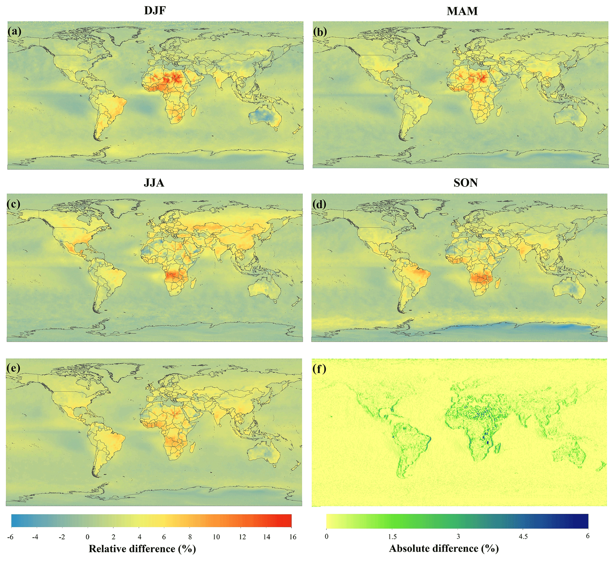
Figure 1AIRS TCO averaged day-to-night relative difference during 2003–2018 for (a) December–January–February, (b) March–April–May, (c) June–July–August, and (d) September–October–November. (e) AIRS TCO 16-year averaged day-to-night relative difference during 2003–2018. (f) Absolute difference between two adjacent pixels at the same latitude in panel (e). Note that the relative difference is calculated as 100 × (daytime − night-time) daytime (in percent, %).
Figure 1e shows the annual mean large differences of AIRS TCO retrievals over deserts, difference patterns over the oceans associated with the Intertropical Convergence Zone (ITCZ), as well as regions with persistent seasonal subtropical stratocumulus fields. The spatial patterns over land mimic regions with low IR surface emissivity and/or regions where IR surface emissivity exhibits large seasonal variations (Feltz et al., 2018). Figure 1f shows absolute differences between all subsequent pixels in the longitudinal direction. The figure reveals significant non-physical TCO changes (discontinuities) for adjacent land–ocean pixels (visible at coast lines running in the north–south direction). All of these effects are important parameters for the retrieval algorithm, but they bear no physical relation to total O3. The observed diurnal cycle in AIRS TCO is related to either the measurements or to the algorithm. If the diurnal cycles in AIRS TCO are related to the retrieval algorithm, it has to be caused by the representation of a process in the algorithm having a diurnal cycle; Smith and Barnet, 2019) argue that the issue does not stem from the algorithm but should be taken into account. Hence, the differences shown in Fig. 1 provide strong indications that the largest AIRS day–night TCO differences are dominated by retrieval artefacts. As such, changes are unphysical, and this confirms the hypothesis that clouds and the surface type (land, desert, vegetation, snow, or ice) affect the AIRS TCO retrievals. Note that TCO day–night differences over land could also be (partly) related to clouds.
The AIRS emissivity retrieval uses the NOAA regression emissivity product as a first guess over land. The NOAA approach is based on clear radiances simulated from the European Centre for Medium-Range Weather Forecasts (ECMWF) forecast and a surface emissivity training data set (Goldberg et al., 2003). The training data set used for the AIRS V4 algorithm has a limited number of soil, ice, and snow types and very little emissivity variability in the training ensemble. In the AIRS V5 version, the regression coefficient set has been upgraded using a number of published emissivity spectra (12 spectra for ice and/or snow and 14 for land) blended randomly for land and ice (Zhou et al., 2008). These improvements generated a better emissivity first guess for use with the AIRS V5 and improved retrievals over the desert regions (Divakarla et al., 2008). In AIRS V6, a surface climatology was constructed from the 2008 monthly MODIS MYD11C3 emissivity product and was extended to the AIRS IR frequency hinge points using the baseline-fit approach described by Seemann et al. (2008). Note that AIRS observations with low information content (especially around the poles) will be drawn to the AIRS a priori value. This AIRS a priori value for O3 is a climatology without diurnal variation. If either the day or night observation has a lower information content than the other, this too can result in a day–night difference. This is probably the reason for the differences in Fig. 1 over pole ice. Nevertheless, using day–night differences for the evaluation of the AIRS V6 O3 product suggests that further refinements for better surface emissivity retrievals are required and that issues related to cloud cover need to be solved.
3.2 MLS O3 retrievals' day–night differences
In order to better understand day–night differences in TCO, we also study day–night changes in the vertical profile of O3 using MLS O3 profile measurements. There are two ways to distinguish between day and night in the observations. When the observation mode is ascending (day), the parameter “AscDescMode” is set to 1; when it is descending (night), the parameter “AscDescMode” is set to −1. Alternatively, the “OrbitGeodeticAngle” parameter of the product embeds the same information, expressed as an angle (Nathaniel J. Livesey, personal communication, 2020).
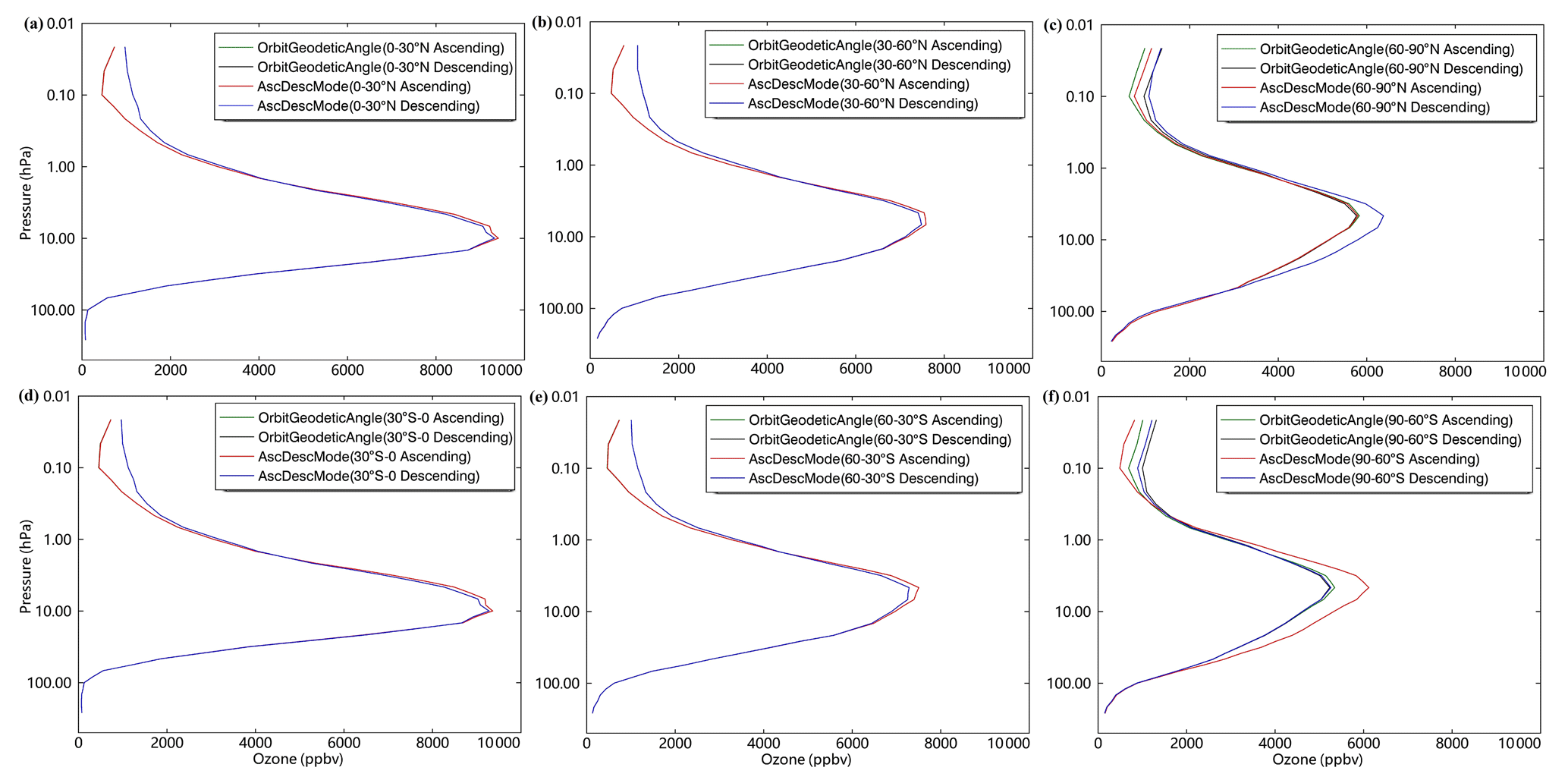
Figure 2Ascending and descending MLS ozone profile between 261 and 0.02 hPa per latitude band (30∘) for 2005–2018: (a) 0–30∘ N, (b) 30–60∘ N, (c) 60–90∘ N, (d) 30∘ S–0, (e) 60–30∘ S, and (f) 90–60∘ S.
Figure 2 shows that the global (60∘ S–60∘ N) differences between the day and night MLS O3 profile occur in the mesosphere (10–0.1 hPa). The O3 mixing ratios are about an order of magnitude larger during night in the mesosphere, which was previously revealed by Huang et al. (2008).
We find an unexpected polar bias distinguished by the “AscDescMode” flag at high latitudes in Fig. 2c and f. On the one hand, the larger differences between the ascending and descending MLS O3 profiles at high latitude extend from the stratosphere to the mesosphere; on the other hand, ascending O3 is smaller than descending O3 at 10 hPa between 60 and 90∘ N in Fig. 2c, which is in contrast with the result of other latitudinal bands.
Day and night MLS O3 profiles distinguished by the “OrbitGeodeticAngle” flag at different latitude bands (30∘) between 60∘ S and 60∘ N display same results as analysis by “AscDescMode”. Figure 2c and f show that the varieties of ascending and descending MLS O3 profiles distinguished by the “OrbitGeodeticAngle” flag at high latitudes are consistent with other regions.
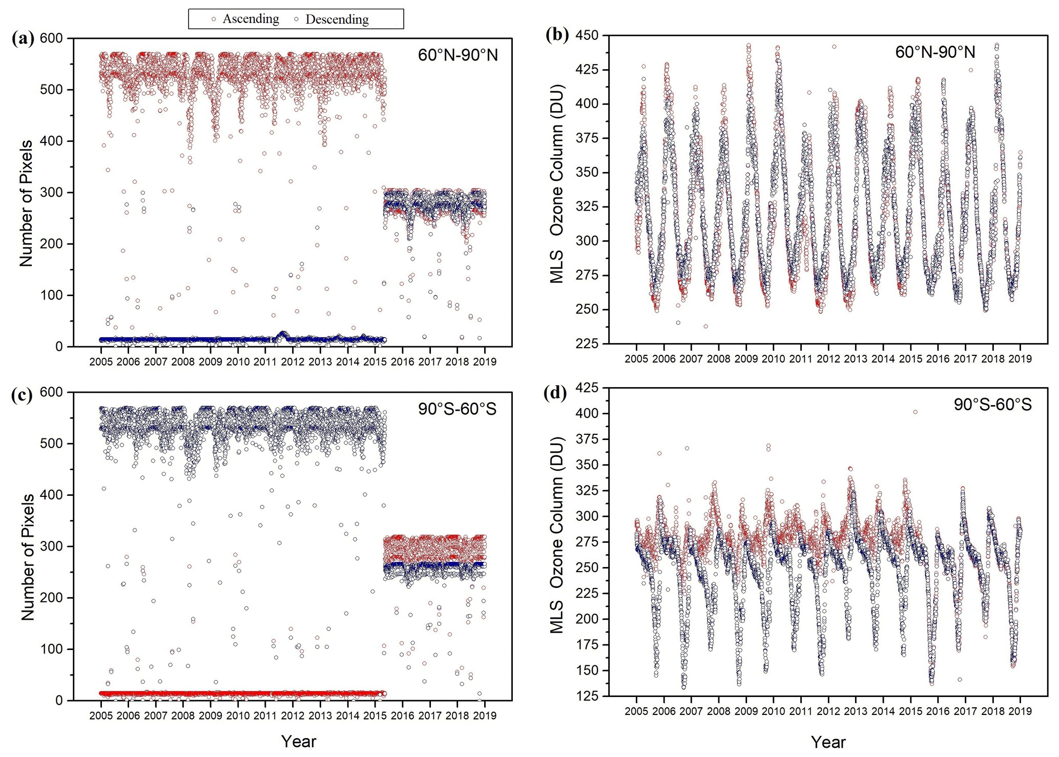
Figure 3(a) Time series of daily number of ascending and descending pixels between 60 and 90∘ N. (b) Time series of daily average ascending and descending MLS SCO between 60 and 90∘ N. Panel (c) is the same as panel (a) but for 90–60∘ S. Panel (d) is the same as panel (b) but for 90–60∘ S.
The MLS O3 profile polar bias mentioned above turns out to be related to an inconsistency in the “AscDescMode” flag of the MLS v4.20 standard O3 product between 90 and 60∘ S and between 60 and 90∘ N. In version v4.22 and later versions this has been fixed. Figure 3a and c show that there is a clear change in the daily number of ascending and descending pixels on 14 May 2015, which is consistent with the change in MLS SCO in Fig. 3b and d. After 14 May 2015 (using version v4.22), the ascending and descending MLS SCO are much closer. For the MLS O3 profile in Fig. 4, differences between ascending and descending MLS O3 profiles at high latitudes for 2016–2018 are very small. Note that the concept day–night has less physical relevance in polar regions due to the presence of the polar day or night. Outside of polar regions many atmospheric parameters show significant 24 h cyclic changes due to differences in heating and cooling between day and night. Due to Earth's orbital inclination, 24 h cyclic variations in atmospheric parameters in polar regions are less significant or even absent.
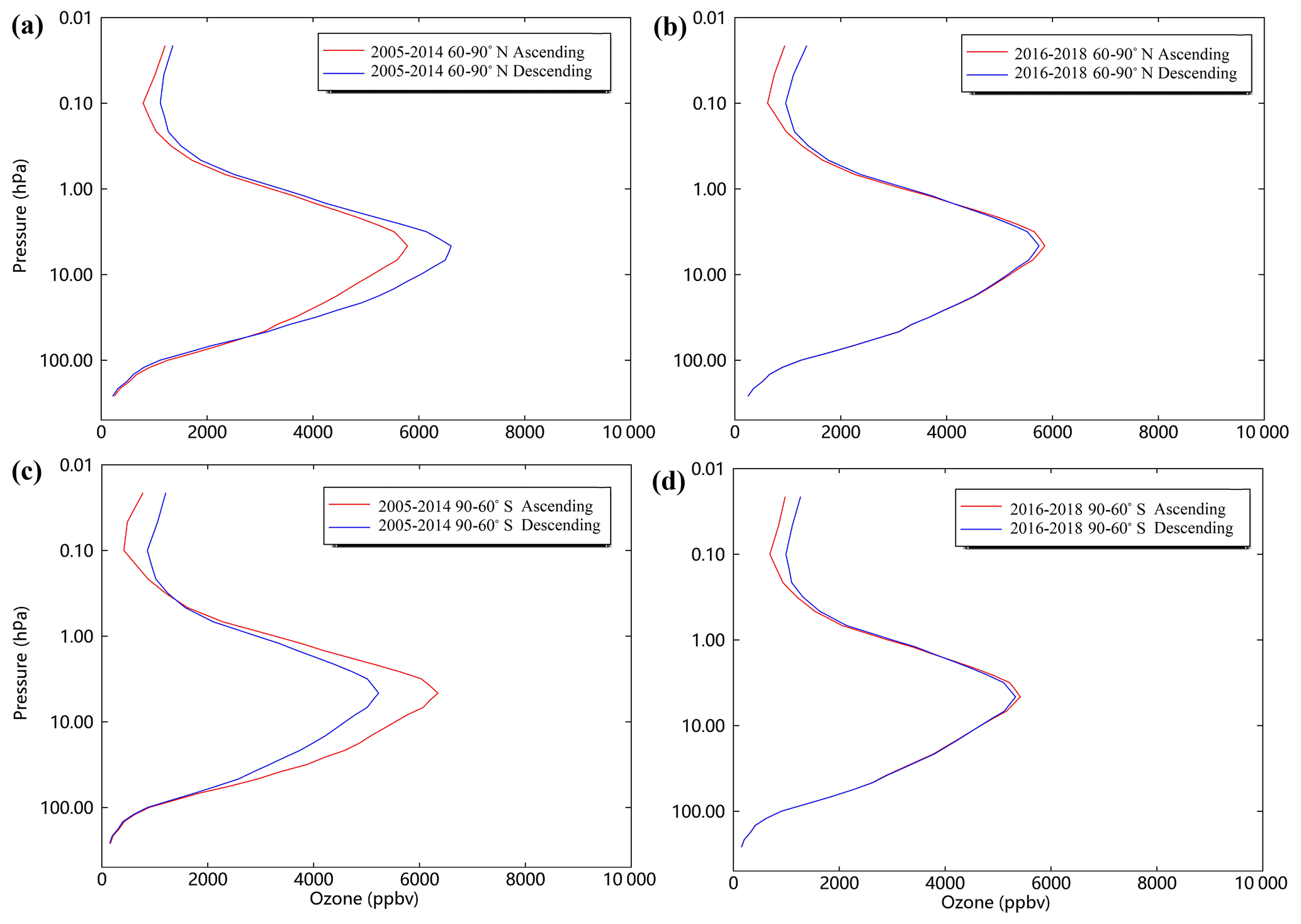
Figure 4(a) Averaged MLS ozone profile between 261 and 0.02 hPa for 2005–2014 from 60 to 90∘ N. (b) Averaged MLS ozone profile between 261 and 0.02 hPa for 2016–2018 from 60 to 90∘ N. Panels (c) is the same as panel (a) but for 90–60∘ S. Panel (d) is the same as panel (b) but for 90–60∘ S.
The O3 retrieval algorithm adopted by the MLS v2.2 products has been validated to be highly accurate using multiple correlative measurements, and the data have been widely used (Jiang et al., 2007; Froidevaux et al., 2008). The MLS v3.3 and v3.4 O3 profiles were reported on a finer vertical grid, and the bottom pressure level with scientifically reliable values (MLS O3 accuracy was estimated at ∼ 20 ppbv + 10 % at 261 hPa) increases from 215 to 261 hPa (Livesey et al., 2015). The latest MLS v4.2x O3 profile used in this study, released in February 2015, was generally similar to the previous version. One of the major improvements of MLS v4.2x was the handling of contamination from cloud signals in trace gas retrievals that resulted in a significant reduction in the number of spurious MLS profiles in cloudy regions and a more efficient screening of cloud-contaminated measurements. Furthermore, the MLS O3 products have been improved through additional retrieval phases and a reduction in interferences from other species (Livesey et al., 2015).
3.3 Comparison between AIRS and MLS O3 retrievals
Figure 5 presents comparison of yearly and monthly averaged SCO for 2005–2018 observed by AIRS and MLS in three latitude bands. Figure 5 explores the seasonality of either AIRS or MLS SCO day–night differences as well as whether the seasonality in day–night SCO varies in unison over the seasons. Figure 5a shows the 14-year average daytime AIRS SCO (250–1 hPa) and MLS SCO (261–0.02 hPa) between 60∘ S and 60∘ N for 2005–2018. The time-averaged MLS SCO column is 260.62 DU and AIRS SCO is 264.24 DU. The average MLS SCO day–night differences for 2005–2018 (0.88 DU) are smaller than the AIRS SCO day–night differences observed for the same time period (5.24 DU). The day–night difference of MLS SCO is 0.79 DU in the mesosphere (10–0.1 hPa) and 0.03 DU in the stratosphere (100–10 hPa). The day–night difference of AIRS SCO is 1.51 DU in the mesosphere (10–1 hPa) and 3.85 DU in the stratosphere (100–10 hPa). Compared with the AIRS SCO day–night differences, the magnitudes of MLS SCO day–night differences in the stratosphere and in the mesosphere are much smaller. It has been pointed out that errors in temperature profiles and water vapour mixing ratios will adversely affect the AIRS O3 retrieval. Significant biases (0 %–100 %) may exist in the region between ∼ 300 and ∼ 80 hPa (Wang et al., 2019; Olsen et al., 2017). AIRS O3 retrievals do not distinguish portions of the O3 profile as being of different qualities, because all AIRS O3 channels sense the surface as well as atmospheric O3. Thus, AIRS O3 retrievals are compromised if the surface is not well characterized (Olsen et al., 2017). In addition, AIRS SCO retrievals show smaller day–night differences in the polar zones (1–2 DU) than between 60∘ S and 60∘ N (4–5 DU). This is related to clouds and the surface type which both affect the AIRS O3 retrievals as mentioned above. Figure 5b shows the monthly 14-year average daytime AIRS SCO and MLS SCO between 60∘ S and 60∘ N for 2005–2018. Seasonal or random changes in clouds and the surface emissivity have a more significant impact on each monthly AIRS SCO retrieval than on the MLS SCO retrieval. Compared with the 60∘ S–60∘ N region, surface types in polar zones are less diverse (snow or ice). Therefore, the monthly 14-year average daytime AIRS SCO and MLS SCO in Fig. 5d and f show similar patterns. Figure 5c–f confirm that both MLS and AIRS can catch SCO seasonality at high latitudes. For AIRS SCO in Fig. 5f, the smallest day–night differences occur in September during the Antarctic O3 hole.
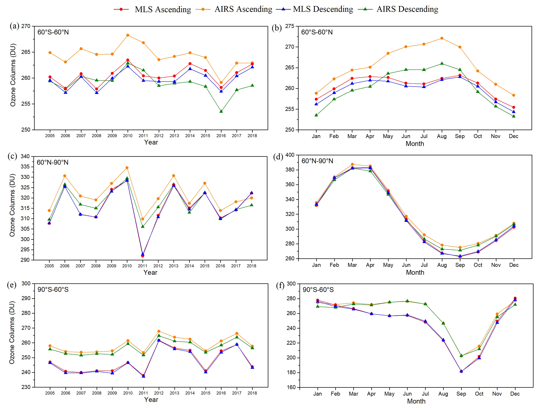
Figure 5Yearly and monthly averaged AIRS SCO and MLS SCO for 2005–2018. AIRS SCOs are calculated from 250 to 1 hPa.
3.4 Day–night difference of equatorial Pacific low-O3 regions
Generally, the Pacific low-O3 region (TCO < 220 DU), called the zonal wave-one feature (Newchurch et al., 2001; Ziemke et al., 2011), exists all year round. It is caused by lower NOx concentrations in this region. Other causes are tropospheric O3 loss related to higher air temperatures and higher water concentrations. High sea surface temperatures favour strong convective activity in the tropical western Pacific, which can lead to low O3 mixing ratios in the convective outflow regions in the upper troposphere in spite of the increased lifetime of odd oxygen (Kley et al., 1996; Rex et al., 2014). A further reduction in the tropospheric O3 burden through bromine and iodine emitted from open-ocean marine sources has been postulated by numerical models (Vogt et al., 1999; von Glasow et al., 2002, 2004; Yang et al., 2005) and observations (Read et al., 2008). However, the day–night differences in this region are expected to be small.
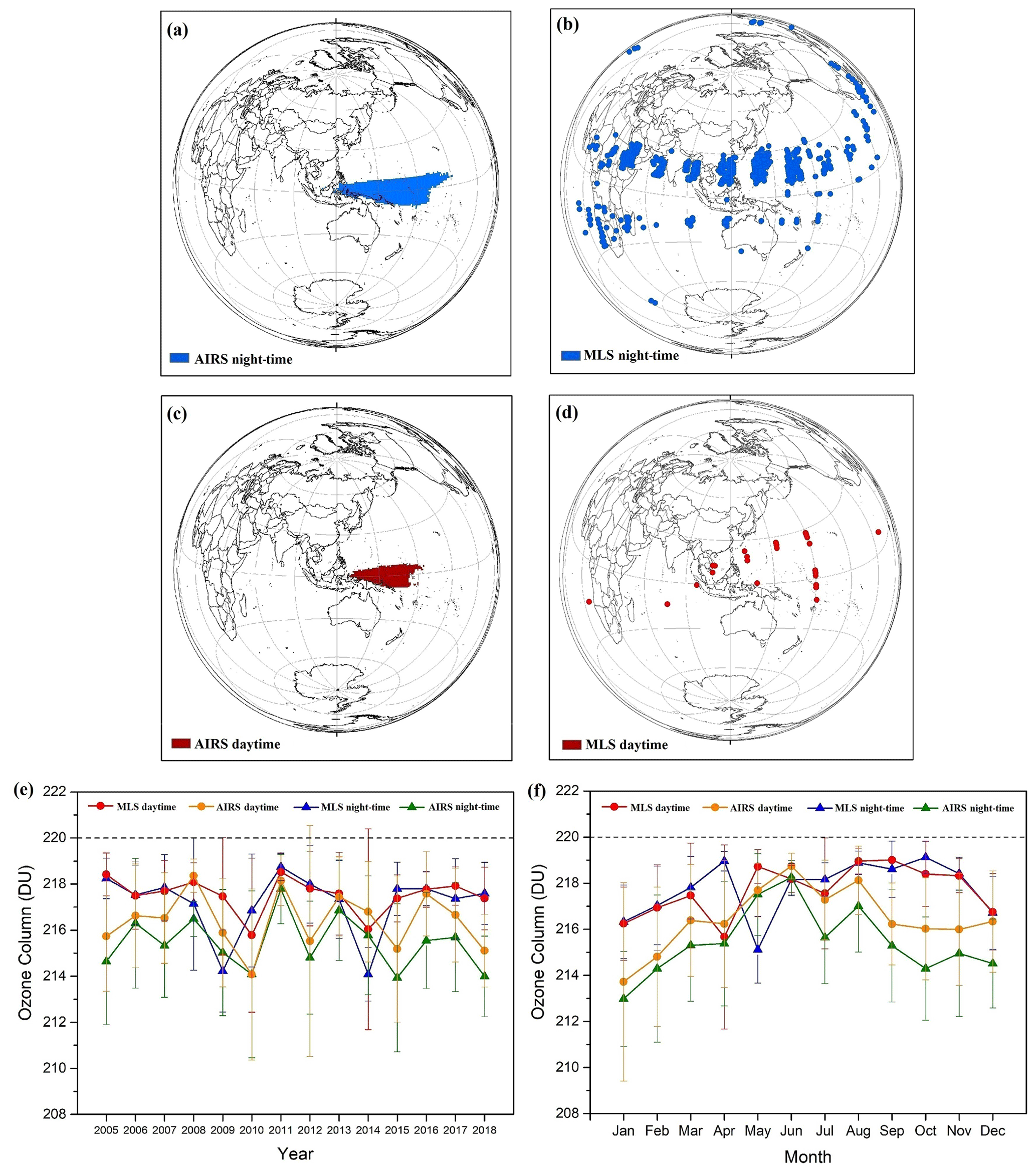
Figure 6Spatial and temporal distribution of the low ozone. (a) Location (composite pixel) of the yearly night-time low ozone from 2005 to 2018 for AIRS TCO. Panel (b) is the same as panel (a) but for MLS SCO. (c) Location (composite pixel) of the yearly daytime low ozone from 2005 to 2018 for AIRS TCO. Panel (d) is the same as panel (c) but for MLS SCO. (e) Yearly averaged AIRS TCO and MLS SCO of the low-ozone regions for 2005–2018. (f) Monthly averaged AIRS TCO and MLS SCO of the low-ozone regions for 2005–2018. Uncertainties represent the standard deviation of the measured values.
Figure 6a and c show that the low-O3 region is mainly located over the western Pacific by AIRS. Rajab et al. (2013) investigated similar low TCO in Malaysia using AIRS data. They found that the highest O3 concentration occurred in April and May, and the lowest O3 concentration occurred during November and December, which is consistent with our results in Fig. 6f. They also found that O3 concentrations exhibited an inverse relationship with rainfall but were positively correlated with temperature. Figure 6b shows that, in addition to the tropical western Pacific, low-O3 regions for MLS appear all over the tropical zone (30∘ S–30∘ N) at night. However, Fig. 6d shows that the occurrence frequency and intensity of daytime low-O3 regions by MLS SCO retrievals drastically reduces and exists mainly in tropical western Pacific. In Fig. 6e and f, yearly and monthly averaged AIRS TCO and MLS SCO of the low-O3 regions show no consistency or regularity. The analysis of daytime MLS SCO of the low-O3 regions is based on only a few observations. We cannot distinguish whether it is an algorithm problem or a chemical mechanism that caused this phenomenon. For AIRS, clouds over oceans may have greater impact on the AIRS TCO retrievals at night. For MLS, more active chemical reactions may occur in these low-O3 regions at night.
For past, current, and future monitoring of atmospheric phenomena like the Pacific tropospheric low-O3 area, it is important that observations are sufficiently accurate. The evaluation of day–night differences in both MLS and AIRS has revealed the existence of biases in the satellite data that are large enough in comparison to expected variations and changes in atmospheric O3 that they may hamper the use of these satellite data studying them.
Comparison of daytime and night-time AIRS TCO has revealed small but not insignificant biases in AIRS TCO. The differences are likely related to surface type (land, desert, vegetation, snow, or ice) and infrared surface emissivity, especially over regions that exhibit smaller infrared emissivity or large seasonal variability in infrared emissivity. Differences were typically of the order of a few percent, which is significant given that long-term changes in TCOs related to anthropogenic emissions of stratospheric O3-depleting substances outside of polar regions are also of the order of a few percent.
Over land, patterns in day–night differences appear to be dominated by the dryness of the surface, suggesting that emissivity may not be well represented or that reduced sensitivity to the lower troposphere during night compared with day over hot surfaces results in a different AIRS TCO. The spatial inhomogeneity of day–night AIRS TCO differences over drier regions points to emissivity dominating these differences. Infrared satellite retrieval artefacts due to land surface emissivity is a well-known phenomenon (Zhou et al., 2013; George et al., 2015; Bauduin et al., 2017).
There were major changes to the surface emissivity retrieval in AIRS V6 compared with previous versions, resulting in a very significant improvement in yield and accuracy for surface temperature and emissivity over land and ice surfaces compared with previous versions. Nevertheless, our results indicate that the AIRS V6 TCO still can be further improved with respect to the representation of infrared emissivity. In addition, AIRS TCO differences over oceans bear a clear cloud cover signature, which is likely related to uncertainties in the representation of clouds in the retrieval algorithm. The latter may also impact AIRS TCO retrievals over land, although detection of cloud features in AIRS TCO day–night differences over land is difficult due to the presence of the land surface emissivity-related bias.
For ocean regions with persistent clouds during day and night (for example, over the ITCZ), Fig. S1 in the Supplement shows that variations in cloud layer height have a greater impact on AIRS TCO day–night differences than variations in the cloud fraction.
Our results do not provide much evidence of another possible causes of day–night differences in AIRS TCO: the photochemical diurnal O3 cycle in the lower troposphere and upper atmosphere. The strongest diurnal O3 effects occur in the boundary layer over land due to night-time surface deposition and daytime photochemical O3 production in the presence of air pollution. In the marine boundary layer, the diurnal O3 cycle is much weaker due to the absence of air pollution and a general slow O3 destruction regime (∼ 10 % d−1). Similarly, in the free troposphere, the diurnal O3 cycle is also weak due to low O3 production rates (generally low levels of pollution relevant for O3 production). Hence, the diurnal O3 cycle in the free troposphere above 750 hPa is negligible (Petetin et al., 2016). In summary, any tropospheric photochemical diurnal O3 cycle effect should resemble some correspondence with air pollution. The day–night differences in AIRS TCO clearly do not resemble patterns of surface air pollution (Fig. 1). MLS day–night differences are confined to the mesosphere (1 hPa and higher). As shown in Smith et al. (2014), the lifetime of O3 due to chemistry is strongly altitude dependent (< 20 min in the upper mesosphere above 0.01 hPa). Only in the mesosphere is the chemical lifetime of O3 long enough to see significant differences between average daytime and night-time concentrations. However, the contribution of mesospheric O3 to MLS SCO is negligible. Thus, the mesospheric diurnal O3 cycle will also have a negligible effect on day–night AIRS TCO differences. In addition, Strode et al. (2019) simulated the global diurnal cycle in the tropospheric O3 columns, and their results indicated that the mean peak-to-peak magnitude of the diurnal variability in tropospheric O3 is approximately 1 DU. Figures S2 to S5 also show that the AIRS TCO retrieval artefacts dominate the day–night variability of tropospheric O3 residuals (TOR = AIRS TCO − MLS SCO).
In summary, our analysis has identified evidence and indications that clouds, land surface infrared emissivity, and the sensitivity of satellite measurements to the lower troposphere influence AIRS satellite TCO observations and has pinpointed areas and processes for algorithm improvement.
The MLS v4.2x was very useful for the verification of daytime and night-time SCO and O3 profiles between 60∘ S and 60∘ N. MLS day–night differences in SCO and O3 profiles show that day–night differences are only small (< 1 DU) and are likely to be in the upper stratosphere and mesosphere. However, an inconsistency was found in the “AscDescMode” flag between 60 and 90∘ N and between 90 and 60∘ S, resulting in inconsistent profiles in these regions before 14 May 2015. In processor version v4.22 and later versions this issue has been fixed, but as it is a relatively small issue, the MLS data set before 2016 has not been reprocessed (confirmed by Nathaniel J. Livesey, personal communication, 2020).
A case study of day–night differences in O3 over the equatorial Pacific revealed that both AIRS and MLS O3 retrievals have biases in comparison to expected variations and changes. Therefore, our results show that maintaining the quality of the satellite observations of stratospheric O3 is highly relevant.
Satellite data sets used in this research can be requested from public sources. AIRS Level 3 data are available online: https://doi.org/10.5067/Aqua/AIRS/DATA303 (AIRS Science Team/Joao Teixeira, 2013a). AIRS Level 2 data are available from https://doi.org/10.5067/Aqua/AIRS/DATA202 (AIRS Science Team/Joao Teixeira, 2013b). MLS Level 2 data can be obtained from https://doi.org/10.5067/Aura/MLS/DATA2017 (Schwartz et al., 2015).
The supplement related to this article is available online at: https://doi.org/10.5194/amt-14-1673-2021-supplement.
WW and JdL provided satellite data, tools, and analysis. RJvdA, JdL, and TC undertook the conceptualization and investigation. WW prepared original draft of the paper. RJvdA and JdL carried out review and editing. JEW checked the English language. All authors discussed the results and commented on the paper.
The authors declare that they have no conflict of interest.
The support provided by the China Scholarship Council (CSC) during Wannan Wang's visit to the Royal Netherlands Meteorological Institute (KNMI) is acknowledged.
This research has been supported by the National Key Research and Development Project of China (grant no. 2017YFC0212302).
This paper was edited by Pawan K. Bhartia and reviewed by Nadia Smith and two anonymous referees.
AIRS Science Team/Joao Teixeira: AIRS/Aqua L3 Daily Standard Physical Retrieval (AIRS-only), 1∘ × 1∘, V006, Goddard Earth Sciences Data and Information Services Center (GES DISC), Greenbelt, Maryland, USA, https://doi.org/10.5067/Aqua/AIRS/DATA303, 2013a.
AIRS Science Team/Joao Teixeira: AIRS/Aqua L2 Standard Physical Retrieval (AIRS-only), V006, Goddard Earth Sciences Data and Information Services Center (GES DISC), Greenbelt, Maryland, USA, https://doi.org/10.5067/Aqua/AIRS/DATA202, 2013b.
American Meteorological Society: https://www.ametsoc.org/index.cfm/ams/publications/bulletin-of-the-american-meteorological-society-bams/state-of-the-climate/ (last access: 13 April 2020), 2011.
Aumann, H. H., Chahine, M. T., Gautier, C., Goldberg, M. D., Kalnay, E., McMillin, L. M., Revercomb, H., Rosenkranz, P. W., Smith, W. L., Staelin, D. H., Strow, L. L., and Susskind, J.: AIRS/AMSU/HSB on the aqua mission: design, science objectives, data products, and processing systems, IEEE T. Geosci. Remote, 41, 253–264, https://doi.org/10.1109/TGRS.2002.808356, 2003.
Aumann, H. H., Broberg, S. E., Manning, E. M., Pagano, T. S., and Wilson, R. C.: Evaluating the Absolute Calibration Accuracy and Stability of AIRS Using the CMC SST, Remote Sens.-Basel, 12, 2743, https://doi.org/10.3390/rs12172743, 2020.
Ball, W. T., Alsing, J., Mortlock, D. J., Staehelin, J., Haigh, J. D., Peter, T., Tummon, F., Stübi, R., Stenke, A., Anderson, J., Bourassa, A., Davis, S. M., Degenstein, D., Frith, S., Froidevaux, L., Roth, C., Sofieva, V., Wang, R., Wild, J., Yu, P., Ziemke, J. R., and Rozanov, E. V.: Evidence for a continuous decline in lower stratospheric ozone offsetting ozone layer recovery, Atmos. Chem. Phys., 18, 1379–1394, https://doi.org/10.5194/acp-18-1379-2018, 2018.
Ball, W. T., Alsing, J., Staehelin, J., Davis, S. M., Froidevaux, L., and Peter, T.: Stratospheric ozone trends for 1985–2018: sensitivity to recent large variability, Atmos. Chem. Phys., 19, 12731–12748, https://doi.org/10.5194/acp-19-12731-2019, 2019.
Barnett, J. J., Houghton, J. T., and Pyle, J. A.: The temperature dependence of the ozone concentration near the stratopause, Q. J. Roy. Meteor. Soc., 101, 245–257, https://doi.org/10.1002/qj.49710142808, 1975.
Bauduin, S., Clarisse, L., Theunissen, M., George, M., Hurtmans, D., Clerbaux, C., and Coheur, P.-F.: IASI's sensitivity to near-surface carbon monoxide (CO): Theoretical analyses and retrievals on test cases, J. Quant. Spectrosc. Ra., 189, 428–440, https://doi.org/10.1016/j.jqsrt.2016.12.022, 2017.
Brown, S. S., Neuman, J. A., Ryerson, T. B., Trainer, M., Dube, W. P., Holloway, J. S., Warneke, C., de Gouw, J. A., Donnelly, S. G., Atlas, E., Matthew, B., Middlebrook, A. M., Peltier, R., Weber, R. J., Stohl, A., Meagher, J. F., Fehsenfeld, F. C., and Ravishankara, A. R.: Nocturnal odd-oxygen budget and its implications for ozone loss in the lower troposphere, Geophys. Res. Lett., 33, L08801, https://doi.org/10.1029/2006GL025900, 2006.
Brühl, C., Drayson, S. R., Russell, J. M., Crutzen, P. J., McInerney, J. M., Purcell, P. N., Claude, H., Gernandt, H., McGee, T. J., and McDermid, I. S.: Halogen Occultation Experiment ozone channel validation, J. Geophys. Res., 101, 10217–10240, https://doi.org/10.1029/95JD02031, 1996.
Chahine, M. T., Pagano, T. S., Aumann, H. H., Atlas, R., Barnet, C., Blaisdell, J., Chen, L., Divakarla, M., Fetzer, E. J., Goldberg, M., Gautier, C., Granger, S., Hannon, S., Irion, F. W., Kakar, R., Kalnay, E., Lambrigtsen, B. H., Lee, S.-Y., Le Marshall, J., McMillan, W. W., McMillin, L., Olsen, E. T., Revercomb, H., Rosenkranz, P., Smith, W. L., Staelin, D., Strow, L. L., Susskind, J., Tobin, D., Wolf, W., and Zhou, L.: AIRS: Improving Weather Forecasting and Providing New Data on Greenhouse Gases, B. Am. Meteorol. Soc., 87, 911–926, https://doi.org/10.1175/BAMS-87-7-911, 2006.
Chapman, S.: A theory of upperatmospheric ozone, Memoirs of the Royal Meteorological Society, 3, 103–125, 1930.
Chipperfield, M. P., Bekki, S., Dhomse, S., Harris, N. R. P., Hassler, B., Hossaini, R., Steinbrecht, W., Thieblemont, R., and Weber, M.: Detecting recovery of the stratospheric ozone layer, Nature, 549, 211–218, https://doi.org/10.1038/nature23681, 2017.
Connor, B. J., Siskind, D. E., Tsou, J., Parrish, A., and Remsberg, E. E.: Ground-based microwave observations of ozone in the upper stratosphere and mesosphere, J. Geophys. Res., 99, 16757–16770, https://doi.org/10.1029/94JD01153, 1994.
Craig, R. A. and Ohring, G.: The temperature dependence of ozone radiational heating rates in the vicinity of the mesopeak, J. Meteorol., 15, 59–62, https://doi.org/10.1175/1520-0469(1958)015<0059:TTDOOR>2.0.CO;2, 1958.
Cunnold, D., Chu, W., Barnes, R., McCormick, M., and Veiga, R.: Validation of SAGE II ozone measurements, J. Geophys. Res., 94, 8447–8460, https://doi.org/10.1029/JD094iD06p08447, 1989.
Divakarla, M., Barnet, C., Goldberg, M., Maddy, E., Irion, F., Newchurch, M., Liu, X. P., Wolf, W., Flynn, L., Labow, G., Xiong, X. Z., Wei, J., and Zhou, L. H.: Evaluation of Atmospheric Infrared Sounder ozone profiles and total ozone retrievals with matched ozonesonde measurements, ECMWF ozone data, and Ozone Monitoring Instrument retrievals, J. Geophys. Res., 113, D15308, https://doi.org/10.1029/2007JD009317, 2008.
Evans, W. and Llewellyn, E.: Measurements of mesospheric ozone from observations of the 1.27 µm band, Radio Sci., 7, 45–50, https://doi.org/10.1029/RS007i001p00045, 1972.
Feltz, M., Borbas, E., Knuteson, R., Hulley, G., and Hook, S.: The Combined ASTER and MODIS Emissivity over Land (CAMEL) Global Broadband Infrared Emissivity Product, Remote Sens.-Basel, 10, 1027, https://doi.org/10.3390/rs10071027, 2018.
Fioletov, V. E., Bodeker, G. E., Miller, A. J., McPeters, R. D., and Stolarski, R.: Global and zonal total ozone variations estimated from ground-based and satellite measurements: 1964–2000, J. Geophys. Res., 107, 4647, https://doi.org/10.1029/2001JD001350, 2002.
Frith, S. M., Bhartia, P. K., Oman, L. D., Kramarova, N. A., McPeters, R. D., and Labow, G. J.: Model-based climatology of diurnal variability in stratospheric ozone as a data analysis tool, Atmos. Meas. Tech., 13, 2733–2749, https://doi.org/10.5194/amt-13-2733-2020, 2020.
Froidevaux, L., Jiang, Y. B., Lambert, A., Livesey, N. J., Read, W. G., Waters, J. W., Browell, E. V., Hair, J. W., Avery, M. A., McGee, T. J., Twigg, L. W., Sumnicht, G. K., Jucks, K. W., Margitan, J. J., Sen, B., Stachnik, R. A., Toon, G. C., Bernath, P. F., Boone, C. D., Walker, K. A., Filipiak, M. J., Harwood, R. S., Fuller, R. A., Manney, G. L., Schwartz, M. J., Daffer, W. H., Drouin, B. J., Cofield, R. E., Cuddy, D. T., Jarnot, R. F., Knosp, B. W., Perun, V. S., Snyder, W. V., Stek, P. C., Thurstans, R. P., and Wagner, P. A.: Validation of aura microwave limb sounder stratospheric ozone measurements, J. Geophys. Res., 113, D15S20, https://doi.org/10.1029/2007JD008771, 2008.
Fu, D., Worden, J. R., Liu, X., Kulawik, S. S., Bowman, K. W., and Natraj, V.: Characterization of ozone profiles derived from Aura TES and OMI radiances, Atmos. Chem. Phys., 13, 3445–3462, https://doi.org/10.5194/acp-13-3445-2013, 2013.
Fu, D., Kulawik, S. S., Miyazaki, K., Bowman, K. W., Worden, J. R., Eldering, A., Livesey, N. J., Teixeira, J., Irion, F. W., Herman, R. L., Osterman, G. B., Liu, X., Levelt, P. F., Thompson, A. M., and Luo, M.: Retrievals of tropospheric ozone profiles from the synergism of AIRS and OMI: methodology and validation, Atmos. Meas. Tech., 11, 5587–5605, https://doi.org/10.5194/amt-11-5587-2018, 2018.
Fussen, D., Vanhellemont, F., Bingen, C., and Chabrillat, S.: Ozone profiles from 30 to 110 km Measured by the Occultation Radiometer Instrument during the period Aug. 1992–Apr. 1993, Geophys. Res. Lett., 27, 3449–3452, https://doi.org/10.1029/2000GL011575, 2000.
George, M., Clerbaux, C., Bouarar, I., Coheur, P.-F., Deeter, M. N., Edwards, D. P., Francis, G., Gille, J. C., Hadji-Lazaro, J., Hurtmans, D., Inness, A., Mao, D., and Worden, H. M.: An examination of the long-term CO records from MOPITT and IASI: comparison of retrieval methodology, Atmos. Meas. Tech., 8, 4313–4328, https://doi.org/10.5194/amt-8-4313-2015, 2015.
Goldberg, M. D., Qu, Y., McMillin, L. M., Wolf, W., Zhou, L., and Divakarla, M.: AIRS near-real-time products and algorithms in support of operational numerical weather prediction, IEEE T. Geosci. Remote, 41, 379–389, https://doi.org/10.1109/TGRS.2002.808307, 2003.
Gunson, M., Farmer, C. B., Norton, R., Zander, R., Rinsland, C. P., Shaw, J., and Gao, B. C.: Measurements of CH4, N2O, CO, H2O, and O3 in the middle atmosphere by the Atmospheric Trace Molecule Spectroscopy Experiment on Spacelab 3, J. Geophys. Res., 95, 13867–13882, https://doi.org/10.1029/JD095iD09p13867, 1990.
Hays, P. and Roble, R. G.: Observation of mesospheric ozone at low latitudes, Planetary Space Science, 21, 273–279, https://doi.org/10.1016/0032-0633(73)90011-1, 1973.
Huang, F. T., Reber, C. A., and Austin, J.: Ozone diurnal variations observed by UARS and their model simulation, J. Geophys. Res., 102, 12971–12985, https://doi.org/10.1029/97JD00461, 1997.
Huang, F. T., Mayr, H. G., Russell, J. M., Mlynczak, M. G., and Reber, C. A.: Ozone diurnal variations and mean profiles in the mesosphere, lower thermosphere, and stratosphere, based on measurements from SABER on TIMED, J. Geophys. Res., 113, A04307, https://doi.org/10.1029/2007JA012739, 2008.
Jiang, Y. B., Froidevaux, L., Lambert, A., Livesey, N. J., Read, W. G., Waters, J. W., Bojkov, B., Leblanc, T., McDermid, I. S., Godin-Beekmann, S., Filipiak, M. J., Harwood, R. S., Fuller, R. A., Daffer, W. H., Drouin, B. J., Cofield, R. E., Cuddy, D. T., Jarnot, R. F., Knosp, B. W., Perun, V. S., Schwartz, M. J., Snyder, W. V., Stek, P. C., Thurstans, R. P., Wagner, P. A., Allaart, M., Andersen, S. B., Bodeker, G., Calpini, B., Claude, H., Coetzee, G., Davies, J., De Backer, H., Dier, H., Fujiwara, M., Johnson, B., Kelder, H., Leme, N. P., König-Langlo, G., Kyro, E., Laneve, G., Fook, L. S., Merrill, J., Morris, G., Newchurch, M., Oltmans, S., Parrondos, M. C., Posny, F., Schmidlin, F., Skrivankova, P., Stubi, R., Tarasick, D., Thompson, A., Thouret, V., Viatte, P., Vömel, H., von der Gathen, P., Yela, M., and Zablocki, G.: Validation of Aura Microwave Limb Sounder Ozone by ozonesonde and lidar measurements, J. Geophys. Res., 112, D24S34, https://doi.org/10.1029/2007JD008776. 2007.
Kaufmann, M., Gusev, O. A., Grossmann, K. U., Martin-Torres, F. J., Marsh, D. R., and Kutepov, A. A.: Satellite observations of daytime and nighttime ozone in the mesosphere and lower thermosphere, J. Geophys. Res., 108, 4272, https://doi.org/10.1029/2002JD002800, 2003.
Kley, D., Crutzen, P. J., Smit, H. G. J., Vomel, H., Oltmans, S. J., Grassl, H., and Ramanathan, V.: Observations of near-zero ozone concentrations over the convective Pacific: Effects on air chemistry, Science, 274, 230–233, https://doi.org/10.1126/science.274.5285.230, 1996.
Koukouli, M. E., Lerot, C., Granville, J., Goutail, F., Lambert, J.-C., Pommereau, J.-P. Balis, D., Zyrichidou, I., Van Roozendael, M., Coldewey-Egbers, M., Loyola, D., Labow, G., Frith, S., Spurr, R., and Zehner, C.: Evaluating a new homogeneous total ozone climate data record from GOME/ERS-2, SCIAMACHY/Envisat, and GOME-2/MetOp-A, J. Geophys. Res.-Atmos., 120, 12296–12312, https://doi.org/10.1002/2015JD023699, 2015.
Livesey, N. J., Filipiak, M. J., Froidevaux, L., Read, W. G., Lambert, A., Santee, M. L., Jiang, J. H., Pumphrey, H. C., Waters, J. W., Cofield, R. E., Cuddy, D. T., Daffer, W. H., Drouin, B. J., Fuller, R. A., Jarnot, R. F., Jiang, Y. B., Knosp, B. W., Li, Q. B., Perun, V. S., Schwartz, M. J., Snyder, W. V., Stek, P. C., Thurstans, R. P., Wagner, P. A., Avery, M., Browell, E. V., Cammas, J.-P., Christensen, L. E., Diskin, G. S., Gao, R.-S., Jost, H.-J., Loewenstein, M., Lopez, J. D., Nedelec, P., Osterman, G. B., Sachse, G. W., and Webster, C. R.: Validation of Aura Microwave Limb Sounder O3 and CO observations in the upper troposphere and lower stratosphere, J. Geophys. Res, 113, D15S02, https://doi.org/10.1029/2007jd008805, 2008.
Livesey, N. J., Read, W. G., Wagner, P. A. Frovideaux, L., Lambert, A., Manney, G. L., Millan, L., Pumphrey, H. C., Santee, M. L., Schwartz, M. J., Wang, S., Fuller, R. A., Jarnot, R. F., Knosp, B. W., and Martinez, E.: Earth Observing System (EOS) Aura Microwave Limb Sounder (MLS) Version 4.2x Level 2 data quality and description document, JPL D-33509 Rev.A, JPL publication, Jet Propulsion Laboratory, California Institute of Technology, Pasadena, California, USA, 2015.
London, J.: Radiative Energy Sources and Sinks in the Stratosphere and Mesosphere, in: Atmospheric Ozone and its Variation and Human Influences, edited by: Nicolet, M. and Aikin, A. C., U.S. Department of Transportation, Washington, D.C., USA, 703, 1980.
Marsh, D. R., Skinner, W. R., Marshall, A. R., Hays, P. B., Ortland, D. A., and Yee, J. H.: High Resolution Doppler Imager observations of ozone in the mesosphere and lower thermosphere, J. Geophys. Res., 107, 4390, https://doi.org/10.1029/2001JD001505, 2002.
Masiello, G., Serio, C., Venafra, S., De Feis, I., and Borbas, E. E.: Diurnal variation in Sahara desert sand emissivity during the dry season from IASI observations, J. Geophys. Res.-Atmos., 119, 1626–1638, https://doi.org/10.1002/jgrd.50863, 2014.
Mlynczak, M. G. and Drayson, S. R.: Calculation of infrared limb emission by ozone in the terrestrial middle atmosphere: 1. Source functions, J. Geophys. Res., 95, 16497–16511, https://doi.org/10.1029/JD095iD10p16497, 1990.
Nalli, N. R., Gambacorta, A., Liu, Q., Tan, C., Iturbide-Sanchez, F., Barnet, C. D., Joseph, E., Morris, V. R., Oyola, M., and Smith, J. W.: Validation of Atmospheric Profile Retrievals from the SNPP NOAA-Unique Combined Atmospheric Processing System, Part 2: Ozone, IEEE T. Geosci. Remote, 56, 598–607, https://doi.org/10.1109/TGRS.2017.2762600, 2018.
Newchurch, M. J., Sun, D., and Kim, J. H.: Zonal wave-1 structure in TOMS tropical stratospheric ozone, Geophys. Res. Lett., 28, 3151–3154, https://doi.org/10.1029/2000GL012315, 2001.
Olsen, E., Fetzer, E., Hulley, G., Kalmus, P., Manning, E., and Wong, S.: AIRS Version 6 Release Level 2 Product User Guide, Jet Propulsion Laboratory, California Institute of Technology, Pasadena, California, USA, 2017.
Pallister, R. C. and Tuck, A. F.: The diurnal variation of ozone in the upper stratosphere as a test of photochemical theory, Q. J. Roy. Meteor. Soc., 109, 271–284, https://doi.org/10.1002/qj.49710946002, 1983.
Parrish, A., Boyd, I. S., Nedoluha, G. E., Bhartia, P. K., Frith, S. M., Kramarova, N. A., Connor, B. J., Bodeker, G. E., Froidevaux, L., Shiotani, M., and Sakazaki, T.: Diurnal variations of stratospheric ozone measured by ground-based microwave remote sensing at the Mauna Loa NDACC site: measurement validation and GEOSCCM model comparison, Atmos. Chem. Phys., 14, 7255–7272, https://doi.org/10.5194/acp-14-7255-2014, 2014.
Petetin, H., Thouret, V., Athier, G., Blot, R., Boulanger, D., Cousin, J.-M., Gaudel, A., Nédélec, P., and Cooper, O.: Diurnal cycle of ozone throughout the troposphere over Frankfurt as measured by MOZAIC-IAGOS commercial aircraft, Elementa: Science of the Anthropocene, 4, 000129, https://doi.org/10.12952/journal.elementa.000129, 2016.
Pittman, J. V., Pan, L. L., Wei, J. C., Irion, F. W., Liu, X., Maddy, E. S., Barnet, C. D., Chance, K., and Gao, R. S.: Evaluation of AIRS, IASI, and OMI ozone profile retrievals in the extratropical tropopause region using in situ aircraft measurements, J. Geophys. Res., 114, D24109, https://doi.org/10.1029/2009JD012493, 2009.
Pommier, M., Clerbaux, C., Law, K. S., Ancellet, G., Bernath, P., Coheur, P.-F., Hadji-Lazaro, J., Hurtmans, D., Nédélec, P., Paris, J.-D., Ravetta, F., Ryerson, T. B., Schlager, H., and Weinheimer, A. J.: Analysis of IASI tropospheric O3 data over the Arctic during POLARCAT campaigns in 2008, Atmos. Chem. Phys., 12, 7371–7389, https://doi.org/10.5194/acp-12-7371-2012, 2012.
Prather, M. J.: Ozone in the upper stratosphere and mesosphere, J. Geophys. Res., 86, 5325–5338, https://doi.org/10.1029/JC086iC06p05325, 1981.
Rajab, J. M., Lim, H., and MatJafri, M.: Monthly distribution of diurnal total column ozone based on the 2011 satellite data in Peninsular Malaysia, The Egyptian Journal of Remote Sensing and Space Science, 16, 103–109, https://doi.org/10.1016/j.ejrs.2013.04.003, 2013.
Read, K. A., Mahajan, A. S., Carpenter, L. J., Evans, M. J., Faria, B. V. E., Heard, D. E., Hopkins, J. R., Lee, J. D., Moller, S. J., Lewis, A. C., Mendes, L., McQuaid, J. B., Oetjen, H., Saiz-Lopez, A., Pilling, M. J., and Plane, J. M. C.: Extensive halogen-mediated ozone destruction over the tropical Atlantic Ocean, Nature, 453, 1232–1235, https://doi.org/10.1038/nature07035, 2008.
Rex, M., Wohltmann, I., Ridder, T., Lehmann, R., Rosenlof, K., Wennberg, P., Weisenstein, D., Notholt, J., Krüger, K., Mohr, V., and Tegtmeier, S.: A tropical West Pacific OH minimum and implications for stratospheric composition, Atmos. Chem. Phys., 14, 4827–4841, https://doi.org/10.5194/acp-14-4827-2014, 2014.
Sakazaki, T., Fujiwara, M., Mitsuda, C., Imai, K., Manago, N., Naito, Y., Nakamura, T., Akiyoshi, H., Kinnison, D., Sano, T., Suzuki, M., and Shiotani, M.: Diurnal ozone variations in the stratosphere revealed in observations from the Superconducting Submillimeter-Wave Limb-Emission Sounder (SMILES) on board the International Space Station (ISS), J. Geophys. Res.-Atmos., 118, 2991–3006, https://doi.org/10.1002/jgrd.50220, 2013.
Schanz, A., Hocke, K., and Kämpfer, N.: Daily ozone cycle in the stratosphere: global, regional and seasonal behaviour modelled with the Whole Atmosphere Community Climate Model, Atmos. Chem. Phys., 14, 7645–7663, https://doi.org/10.5194/acp-14-7645-2014, 2014.
Schwartz, M., Froidevaux, L., Livesey, N., and Read, W.: MLS/Aura Level 2, Ozone (O3) Mixing Ratio V004, Goddard Earth Sciences Data and Information Services Center (GES DISC), Greenbelt, Maryland, USA, https://doi.org/10.5067/Aura/MLS/DATA2017, 2015.
Seemann, S. W., Borbas, E. E., Knuteson, R. O., Stephenson, G. R., and Huang, H.-L.: Development of a global infrared land surface emissivity database for application to clear sky sounding retrievals from multispectral satellite radiance measurements, J. Appl. Meteorol. Clim., 47, 108–123, https://doi.org/10.1175/2007JAMC1590.1, 2008.
Simpson, D., Arneth, A., Mills, G., Solberg, S., and Uddling, J.: Ozone – the persistent menace: interactions with the N cycle and climate change, Curr. Opin. Env. Sust., 9–10, 9–19, https://doi.org/10.1016/j.cosust.2014.07.008, 2014.
Sitnov, S. A. and Mokhov, I. I.: Satellite-derived peculiarities of total ozone field under atmospheric blocking conditions over the European part of Russia in summer 2010, Russ. Meteorol. Hydro.+, 41, 28–36, https://doi.org/10.3103/S1068373916010040, 2016.
Smith, A. K. and Marsh, D. R.: Processes that account for the ozone maximum at the mesopause, J. Geophys. Res., 110, D23305, https://doi.org/10.1029/2005JD006298, 2005.
Smith, A. K., Lopez-Puertas, M., Funke, B., Garcia-Comas, M., Mlynczak, M. G., and Holt, L. A.: Nighttime ozone variability in the high latitude winter mesosphere, J. Geophys. Res.-Atmos., 119, 13547–13564, https://doi.org/10.1002/2014JD021987, 2014.
Smith, N. and Barnet, C. D.: Uncertainty Characterization and Propagation in the Community Long-Term Infrared Microwave Combined Atmospheric Product System (CLIMCAPS), Remote Sens.-Basel, 11, 1227, https://doi.org/10.3390/rs11101227, 2019.
Strode, S. A., Ziemke, J. R., Oman, L. D., Lamsal, L. N., Olsen, M. A., and Liu, J.: Global changes in the diurnal cycle of surface ozone, Atmos. Environ., 199, 323–333, https://doi.org/10.1016/j.atmosenv.2018.11.028, 2019.
Susskind, J., Barnet, C. D., and Blaisdell, J. M.: Retrieval of atmospheric and surface parameters from AIRS/AMSU/HSB data in the presence of clouds, IEEE T. Geosci. Remote, 41, 390–409, 2003.
Susskind, J., Blaisdell, J. M., Iredell, L., and Keita, F.: Improved Temperature Sounding and Quality Control Methodology Using AIRS/AMSU Data: The AIRS Science Team, Version 5, Retrieval Algorithm, IEEE T. Geosci. Remote, 49, 883–907, https://doi.org/10.1109/TGRS.2010.2070508, 2011.
Susskind, J., Blaisdell, J. M., and Iredell, L.: Improved methodology for surface and atmospheric soundings, error estimates, and quality control procedures: the atmospheric infrared sounder science team, version-6, retrieval algorithm, J. Appl. Remote Sens., 8, 084994, https://doi.org/10.1117/1.JRS.8.084994, 2014.
Tian, B., Yung, Y. L., Waliser, D. E., Tyranowski, T., Kuai, L., Fetzer, E. J., and Irion, F. W.: Intraseasonal variations of the tropical total ozone and their connection to the Madden-Julian Oscillation: The MJO in tropical total ozone, Geophys. Res. Lett., 34, L08704, https://doi.org/10.1029/2007GL029451, 2007.
Velders, G. J., Andersen, S. O., Daniel, J. S., Fahey, D. W., and McFarland, M.: The importance of the Montreal Protocol in protecting climate, P. Natl. Acad. Sci. USA, 104, 4814–4819, https://doi.org/10.1073/pnas.0610328104, 2007.
Vogt, R., Sander, R., Von Glasow, R., and Crutzen, P. J.: Iodine chemistry and its role in halogen activation and ozone loss in the marine boundary layer: A model study, J. Atmos. Chem., 32, 375–395, https://doi.org/10.1023/A:1006179901037, 1999.
von Glasow, R., Sander, R., Bott, A., and Crutzen, P. J.: Modeling halogen chemistry in the marine boundary layer, 1. Cloud-free MBL, J. Geophys. Res., 107, 4341, https://doi.org/10.1029/2001JD000942, 2002.
von Glasow, R., von Kuhlmann, R., Lawrence, M. G., Platt, U., and Crutzen, P. J.: Impact of reactive bromine chemistry in the troposphere, Atmos. Chem. Phys., 4, 2481–2497, https://doi.org/10.5194/acp-4-2481-2004, 2004.
Wang, H., Chai, S., Tang, X., Zhou, B., Bian, J., Vömel, H., Yu, K., and Wang, W.: Verification of satellite ozone/temperature profile products and ozone effective height/temperature over Kunming, China, Sci. Total Environ., 661, 35–47, https://doi.org/10.1016/j.scitotenv.2019.01.145, 2019.
Waters, J. W., Froidevaux, L., Harwood, R. S., Jarnot, R. F., Pickett, H. M., Read, W. G., Siegel, P. H., Cofield, R. E., Filipiak, M. J., and Flower, D. A.: The earth observing system microwave limb sounder (EOS MLS) on the Aura satellite, IEEE T. Geosci. Remote, 44, 1075–1092, https://doi.org/10.1109/TGRS.2006.873771, 2006.
Weeks, L., Good, R., Randhawa, J., and Trinks, H.: Ozone measurements in the stratosphere, mesosphere, and lower thermosphere during Aladdin 74, J. Geophys. Res., 83, 978–982, https://doi.org/10.1029/JA083iA03p00978, 1978.
WMO: Scientific Assessment of Ozone Depletion: 2010, Global Ozone Research and Monitoring Project-Report, No. 52, World Meteorological Organization (WMO), Geneva, Switzerland, 516 pp., 2011.
WMO: Scientific Assessment of Ozone Depletion: 2014, World Meteorological Organization, Global Ozone Research and Monitoring Project-Report, No. 55, World Meteorological Organization (WMO), Geneva, Switzerland, 416 pp., 2014.
WMO: Scientific Assessment of Ozone Depletion: 2018, Global Ozone Research and Monitoring Project-Report, No. 58, World Meteorological Organization (WMO), Geneva, Switzerland, 588 pp., 2018.
Yang, X., Cox, R. A., Warwick, N. J., Pyle, J. A., Carver, G. D., O'Connor, F. M., and Savage, N. H.: Tropospheric bromine chemistry and its impacts on ozone: A model study, J. Geophys. Res., 110, D23311, https://doi.org/10.1029/2005JD006244, 2005.
Zhou, D. K., Larar, A. M., and Liu, X.: MetOp-A/IASI Observed Continental Thermal IR Emissivity Variations, IEEE J. Sel. Top. Appl., 6, 1156–1162, https://doi.org/10.1109/JSTARS.2013.2238892, 2013.
Zhou, L., Goldberg, M., Barnet, C., Cheng, Z., Sun, F., Wolf, W., King, T., Liu, X., Sun, H., and Divakarla, M.: Regression of surface spectral emissivity from hyperspectral instruments, IEEE T. Geosci. Remote, 46, 328–333, https://doi.org/10.1109/TGRS.2007.912712, 2008.
Ziemke, J. R., Chandra, S., Labow, G. J., Bhartia, P. K., Froidevaux, L., and Witte, J. C.: A global climatology of tropospheric and stratospheric ozone derived from Aura OMI and MLS measurements, Atmos. Chem. Phys., 11, 9237–9251, https://doi.org/10.5194/acp-11-9237-2011, 2011.
Zommerfelds, W., Kunzi, K., Summers, M., Bevilacqua, R., Strobel, D., Allen, M., and Sawchuck, W.: Diurnal variations of mesospheric ozone obtained by ground-based microwave radiometry, J. Geophys. Res., 94, 12819–12832, https://doi.org/10.1029/JD094iD10p12819, 1989.
AscDescModeflag of the MLS v4.20 standard O3 product for 90–60° S and 60–90° N, resulting in inconsistent O3 profiles in these regions before May 2015.