Measurement characteristics of an airborne microwave temperature profiler (MTP)

The microwave temperature profiler (MTP), an airborne passive microwave radiometer, measures radiances, recorded as counts and calibrated to brightness temperatures, in order to estimate temperature profiles around flight altitude. From these data, quantities such as potential temperature gradients and static stability, indicating the state of the atmosphere, can be derived and used to assess important dynamical processes (e.g., gravity waves or stability assessments). DLR has acquired a copy of the MTP from NASA–JPL, which was designed as a wing-canister instrument and is deployed on the German High Altitude LOng range research aircraft (HALO). For this instrument a thorough analysis of instrument characteristics has been made in order to correctly determine the accuracy and precision of MTP measurements.

Using a laboratory setup, the frequency response function and antenna diagram of the instrument were carefully characterized. A cold chamber was used to simulate the changing in-flight conditions and to derive noise characteristics as well as reliable calibration parameters for brightness temperature calculations, which are compared to those calculated from campaign data.

The MTP shows quite large changes in the instrument state, imposing considerable changes in calibration parameters over the course of a single measurement flight; using a built-in heated target for calibration may yield large errors in brightness temperatures due to a misinterpretation of the measured absolute temperature. Applying the corrections presented herein to the calibration parameter calculations, the measurement noise becomes the dominant source of uncertainty and it is possible to measure the brightness temperatures around flight level (closely related to the absolute temperature close to the instrument) with a precision of 0.38 K. Furthermore, radiative transfer simulations, using the Py4CAtS package in a pencil-beam approach, indicate that the altitude range of the sensitivity of the MTP instrument can be increased by applying a modified measurement strategy.

This is the first time such an extensive characterization of an MTP instrument, including a thorough calibration strategy assessment, has been published. The presented results, relevant for the wing-canister design of the MTP instrument, are important when processing MTP data: knowledge of the relevant uncertainties and instrument characteristics is essential for retrieval setup and is mandatory to correctly identify and interpret significant atmospheric temperature fluctuations.

1 Introduction

Aircraft campaigns have long been used to study atmospheric composition and dynamics. Here, one important variable to be determined is the atmospheric temperature, ideally not only at flight level, as provided in high resolution by the standard aircraft instrumentation. For this measurement it is desirable to use a remote sensing technique that provides good horizontal and vertical resolution. A variety of instruments and techniques exists; many of them are used in ground-based setups or installed on satellites. For aircraft instruments, the line of sight is always an important factor, as is the ability to record data fast (providing high horizontal resolution). It is desirable to use a robust instrument design able to perform despite frequent changes in conditions due to flight patterns and geographical regions of deployment. On the German High Altitude LOng range research aircraft (HALO; Krautstrunk and Giez, 2012), the microwave temperature profiler (MTP; Denning et al., 1989) complements other instruments such as the Basic HALO Measurement and Sensor System (BAHAMAS), which measures the temperature amongst other parameters at flight level, and dropsondes. In contrast to such in situ instruments, the MTP scans through the atmosphere at different viewing directions, providing temperature profile information at, above, and below flight level. A copy of this compact wing-canister instrument, which was originally designed by NASA–JPL, has been transferred to DLR and was modified and certified for operation on HALO. On that aircraft it constitutes a valuable addition to the scientific payload as the data recorded by the MTP facilitate the interpretation of trace gas measurements taken during flight (e.g., by indicating tropopause height and static stability) and increase the atmospheric region over which information can be gathered. Combining MTP and dropsonde data (e.g., for cross-validation) or exploiting the synergy with the airborne multi-wavelength water vapor differential absorption lidar (WALES; Wirth et al., 2009) offers the opportunity to increase the insight into atmospheric processes targeted during measurement flights. Its observation range at, above, and below flight level plus its small size and weight clearly set the MTP apart from the HALO Microwave Package (HAMP; Mech et al., 2014), which is another optional instrument package deployable in HALO's belly pod capable of retrieving both humidity and temperature profiles, as well as the liquid water path (Jacob et al., 2019), below flight level by means of passive microwave radiometry.

The value of MTP data is also demonstrated by its continued use in many aircraft campaigns. Since its invention in the late 1970s, the MTP has been deployed in a number of aircraft campaigns (Mahoney and Denning, 2009) and continues to be developed to meet today's standards of technical requirements and data recording. In the past, MTP data have been used to interpret in situ measurements of trace gases (e.g., Marcy et al., 2007; Thornton et al., 2007; Spinei et al., 2015) and aerosols, (e.g., Gamblin et al., 2006; Popp et al., 2006; Schwarz et al., 2008), as well as to assist the study of cloud physics (e.g., Corti et al., 2008; Jensen et al., 2010; Schumann et al., 2017; Urbanek et al., 2017) and dynamics in the atmosphere (e.g., Tuck et al., 1997, 2003; Dörnbrack et al., 2002; Sitnikova et al., 2009). Other studies, focusing exclusively on MTP data, include the derivation of the boundary layer height from MTP potential temperature isentropes (Nielsen-Gammon et al., 2008), investigation of mixing processes within the polar vortex (Hartmann et al., 1989), and calculation of the cold point temperature and mesoscale temperature fluctuations, derived as the difference to the mission average temperature, in the upper troposphere and lower stratosphere (UTLS) in connection to tropical weather disturbances (Davis et al., 2014). Furthermore, MTP measurements have been utilized to investigate gravity waves in the atmosphere. Studies have focused on general overviews (Gary, 2006, 2008), the formation of polar stratospheric clouds (PSCs; Murphy and Gary, 1995; Tabazadeh et al., 1996), and the characterization of gravity waves encountered during flight (Gary, 1989; Chan et al., 1993; Dean-Day et al., 1998; Wang et al., 2006). Based on these mesoscale temperature fluctuation analyses, a number of modeling studies aimed at improving the understanding and numerical description of atmospheric gravity waves were published, including studies by Bacmeister et al. (1990, 1996, 1999), Pfister et al. (1993), Cho et al. (1999), Leutbecher and Volkert  (2000), Dörnbrack et al. (2002), and Eckermann et al. (2006). Especially for studies focusing on mesoscale temperature fluctuations or vertical temperature gradients, precise knowledge of the instrument characteristics, such as intrinsic noise and the precision of the measurements, is necessary, e.g., when identifying potential gravity wave signals within the time series of MTP data. Knowing the true range of sensitivity is also necessary to understand the shape and characteristic structures within the retrieved temperature profiles.

Despite the continuous use of data from various MTP instruments in many studies over the past decades, a thorough instrument characterization and estimation of measurement accuracy (i.e., the deviation from the true value; mostly influenced by systematic errors) and precision (i.e., the spread of the individual measurements; mostly influenced by random errors, such as measurement noise) have not yet been published. For the first time, this study presents a thorough investigation of relevant instrument characteristics of the HALO MTP instrument. All measurements shown in the following sections are important to correctly choose retrieval settings and interpret time series of MTP data. They were conducted without disassembling the instrument, provided that the hardware characteristics are comparable to previous mission deployments, thereby guaranteeing the continued airworthiness of the instrument on the HALO aircraft. Knowing the instrument characteristics is the foundation for correct analysis and interpretation of data recorded by the HALO MTP. The following sections present a brief description of the instrument and its measuring principle (Sect. 2), measurements of the instrument response function, the antenna diagram, and other inherent characteristics, such as measurement noise (Sect. 3), and a discussion of calibration strategies to determine the best practice (Sect. 4), including a discussion of the influence of flight-level changes on the instrument state and measurement performance. Further error sources and some discussion of possible improvements to the measurement strategy are presented in Sect. 5. The findings are summarized in Sect. 6.

2 Instrument description

The first MTP instrument was developed in the late 1970s by Bruce Gary and Richard Denning at the Jet Propulsion Laboratory (NASA–JPL) for research on clear-air turbulence (CAT; Gary, 1989). Since its first deployment in the Stratospheric–Tropospheric Exchange Project (STEP) in Australia in 1987, the MTP has been widely regarded as an instrument providing valuable background information on the state of the atmosphere, and several instrument designs have been realized. The latest development is the MTP as a wing-canister instrument (see Fig. 1a), which can be mounted underneath the wing of a research aircraft (e.g., Haggerty et al., 2014). Two such instruments were built. One has been deployed on the NCAR GV since 2008 (e.g., Lim et al., 2013; Davis et al., 2014; Haggerty et al., 2014), and the other (hereafter referred to as the HALO MTP) was acquired by DLR and has been flown on the German research aircraft HALO (Krautstrunk and Giez, 2012). This design was first introduced in 2008. Details of the instrument design and some discussion on standard measurement settings can be found in Mahoney and Denning (2009) and Lim et al. (2013).

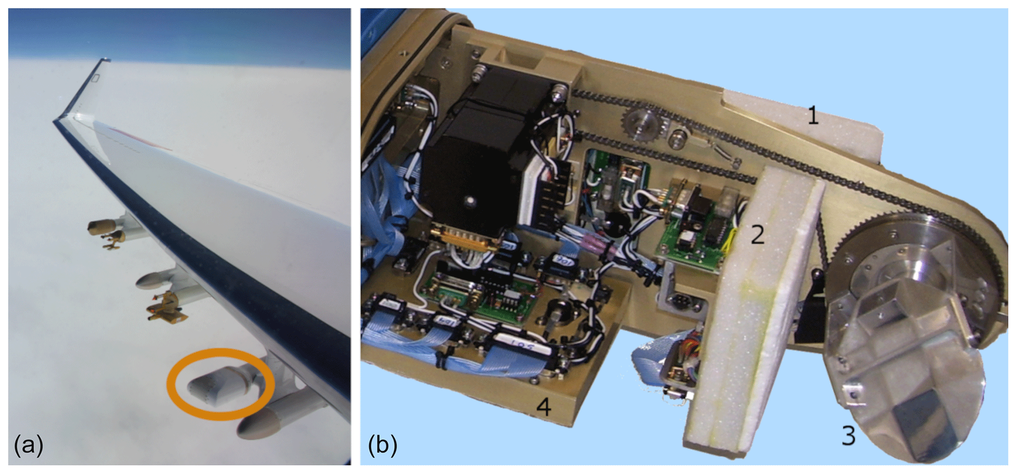
Figure 1 HALO MTP instrument. (a) Position of the MTP underneath the wing of the HALO aircraft. (b) MTP sensor unit in the lab. Marked with numbers are the radiometer unit (1), the hot calibration target (2), the rotating mirror (3), and the electronic unit (4), which contains various temperature sensors such as the scanning unit temperature and the pod air temperature sensor.

Table 1 MTP instrument: components and settings.

In the following, an overview of the characteristics of this specific version of MTP instruments is given, starting with a brief introduction of the measurement principle followed by a description of specific radiometric hardware (see also Table 1) built into the HALO MTP. All results in the following sections are representative of this specific MTP instrument design.

2.1 Measurement principle

The concept of measurements by the MTP as a passive total-power radiometer (Denning et al., 1989; Ulaby et al., 1981) is straightforward. The MTP records thermal radiation mainly emitted by oxygen molecules in the atmosphere. Like many radiometers measuring atmospheric temperature, the MTP uses absorption lines of the 60 GHz oxygen complex (“V band”), which are caused by magnetic dipole transitions (Liebe et al., 1992). Passive radiometers pick up the energy transported by the photons emitted in these transitions. In this part of the spectrum, the Rayleigh–Jeans relation (e.g., Ulaby et al., 1981) can be used to describe the source function of the radiance picked up by the MTP:

$$\begin{array}{}\text{(1)}& B\left(\mathit{\nu },T\right)={\displaystyle \frac{\mathrm{2}h{\mathit{\nu }}^{\mathrm{3}}}{c^{\mathrm{2}}}}\cdot {\displaystyle \frac{\mathrm{1}}{\exp \left(\frac{h\mathit{\nu }}{k_{\mathrm{B}}T}\right)-\mathrm{1}}}\cong \mathrm{2}{\displaystyle \frac{{\mathit{\nu }}^{\mathrm{2}}}{c^{\mathrm{2}}}}\cdot k_{\mathrm{B}}T,\end{array}$$

in which the measured radiance is equal to the brightness B of a black body described by Planck's law. This equation implies a linear relationship between the measured radiance and the temperature T of the black body source at a certain frequency ν using the Planck constant, h, velocity of light, c, and the Boltzmann constant k_B. This temperature, T, is referred to as brightness temperature (T_B), which is the temperature of on an ideal black body emitting the equivalent radiance. The recorded T_Bs have to be converted to absolute temperature profiles by using a retrieval algorithm that utilizes forward radiative transfer calculations, in which, ideally, all possible impacts on the measured radiance (e.g., water vapor, nitrous oxide, or hydrometeors) have to be considered. For correct interpretation of the fluctuations found in the retrieved temperature fields, it is necessary to have precise knowledge of the instrument characteristics, such as the instrument response function, antenna diagram (see Sect. 3), and the precision and accuracy of the brightness temperature measurements that are input to the retrieval algorithm (see Sect. 4).

In the MTP instrument, a horn antenna guides the incoming atmospheric radiation and, together with the hyperbolic shape of the rotating mirror, determines the spatial response function. The measurements are based on the heterodyne principle, which means that through mixing with a defined frequency, the local oscillator frequency (LO), the incoming signal is converted to an interim frequency (IF) near base band. Both difference frequencies below and above the LO frequency are down-converted to the IF in the double-side-band receiver. Low-pass filtering suppresses any incoming radiation outside the IF bandwidth of 200 MHz such that the symmetric spectrum around the current LO frequency is measured with only a minor gap of approximately 20 MHz at the LO frequency. The IF signal is converted to a voltage, which is proportional to the squared input amplitude, representing the power. This voltage is finally translated to a digital count number, stored in the MTP data file, and later converted into a brightness temperature through calibration (see Sect. 4). The physical temperatures of the important radiometric parts of the radiometer, such as the mixer, synthesizer, amplifiers, and the electronics, are stabilized to minimize the influence of the changing conditions during a research flight on the instrument state and to protect the electronic parts from malfunction due to condensation (see Mahoney and Denning, 2009, for further details).

Using a rotating mirror in front of the instrument's feed antenna (number 3 in Fig. 1b), the direction from which the radiation is collected can be changed. Moving through a single set of elevation angles, as well as the set of frequency channels at each of those elevation angles, is referred to in the following as a measurement “cycle”. This procedure enhances the vertical resolution of measurements in comparison to non-scanning measurements, which derive altitude information solely from exploiting frequency-dependent differences in the optical depth of the atmosphere. The MTP combines both principles. In its standard deployment settings, as programmed in the original JPL instrument software, 10 viewing angles are used during one measurement cycle: five above the horizon, four below, and one pointing exactly towards the horizon. At each angle, measurements at three frequency channels, corresponding to the frequencies of three strong oxygen absorption lines, are subsequently performed (see Table 1) before moving to the next elevation.

Furthermore, a calibration target is built into the instrument (number 2 in Fig. 1b), to which the mirror points after each cycle of atmospheric measurements. The target itself consists of carbon–ferrite on an aluminum plate, which is heated to a constant temperature (approximately 45 ^∘C) using two conventional power resistors. The calibration target is surrounded by a 1 in. thick Styrofoam insulation, which is transparent for microwave radiation. The signals recorded while pointing towards the heated target are combined with a noise diode (ND) signal and used for calibration (see Sect. 4) to convert the measured signal to a T_B, which is usually not equal to the outside air temperature, since the measured signal is influenced by multiple layers of the atmosphere. To derive absolute temperature from the radiation measurement, radiative transfer calculations have to be carried out and compared to the measured radiances by applying a retrieval algorithm in post-processing. The instrument characteristics presented in the following sections of this work all correspond to the raw measurements or the brightness temperatures, which are input to such a retrieval algorithm. However, a discussion of retrieval algorithms and related uncertainties is beyond the scope of this paper.

2.2 Specific wing-canister instrument hardware characteristics

Differences to older instrument designs are presented in Lim et al. (2013) and Haggerty et al. (2014). The most important upgrade is that the LO is now defined as a frequency near (or ideally at) an oxygen absorption line center so that the two flanks that are measured belong to the same line, which lowers the brightness temperature error, as discussed in Mahoney and Denning (2009) and Lim et al. (2013). The instrument is pointing forward, measuring the temperatures of air masses in front of the aircraft. The filter bandwidth of the HALO MTP is fixed to ±200 MHz around the LO, with a gap of approximately 20 MHz at the line center (see Fig. 2a). The synthesizer used to generate the LO for down-conversion of the signal can be tuned between 12 and 16 GHz. The synthesizer output is doubled twice, potentially allowing for a frequency range of 48 to 64 GHz for atmospheric measurements. The preset (“standard”) set of LO frequencies used was chosen based on the considerations presented in Mahoney and Denning (2009) and Lim et al. (2013). This set of frequencies is used for this study.

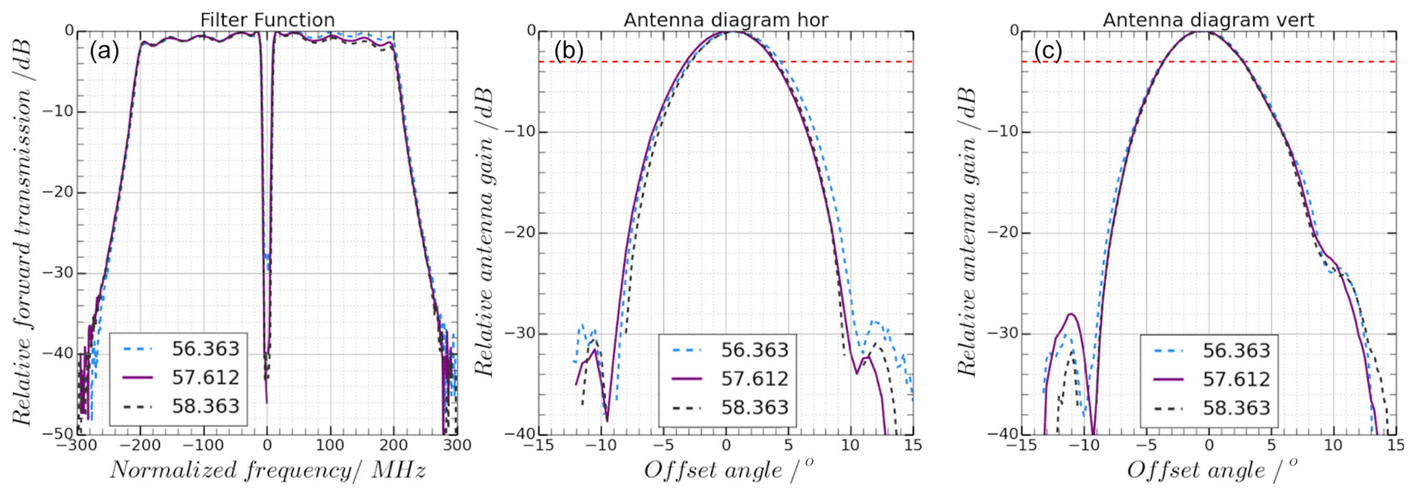
Figure 2 HALO MTP filter functions (a) and antenna diagram of the horizontal (b) and vertical (c) plane recorded at standard measurement frequencies. Red dashed lines indicate the half-maximum value. All data are normalized so that the maximum value shown is 0.

Two significant modifications to the original instrument were made by DLR: an embedded computer and an inertial measurement system including a Global Positioning System (GPS) antenna. In the original setup a Visual Basic software package was provided by NASA–JPL to run the instrument during research flights. With the onboard computer and integration of the inertial sensor, this software was translated to a LabView code, which was adjusted to use the additional data provided by the inertial sensor. With those modifications, the HALO MTP can be operated autonomously, i.e., independent from a connection to a cabin computer, which is still provided and can be used, e.g., to adjust settings during research flights using the HALO LAN network.

The HALO MTP was first deployed during the Midlatitude Cirrus Experiment (ML CIRRUS) in 2014 (Voigt et al., 2017). The focus of this mission was to probe natural cirrus clouds and contrail cirrus throughout various stages of their life cycles. The MTP was part of the wing-probe instrumentation and recorded data during all mission flights. In total, the HALO MTP produced almost 63 h of data during 13 mission flights, recording 17 476 individual measurement cycles. Data from this campaign will be used to derive the HALO MTP noise characteristics and in the investigation of calibration methods in the following sections.

3 Characteristics of the wing-canister MTP flown on HALO

To retrieve absolute temperature profiles from the MTP measurements, radiative transfer calculations are carried out to model the measured radiance in a defined atmospheric state. To correctly do so, the instrument transmission function (see Fig. 2a) has to be known. This function is defined by the instrument's filter function, which determines which part of the recorded spectrum is used in data processing. Moreover, the antenna diagram (see Fig. 2) shows how sensitive the receiver is to the different directions it is pointing towards. Both the filter functions and the antenna diagram have been measured in a stable laboratory environment (Sect. 3.1).

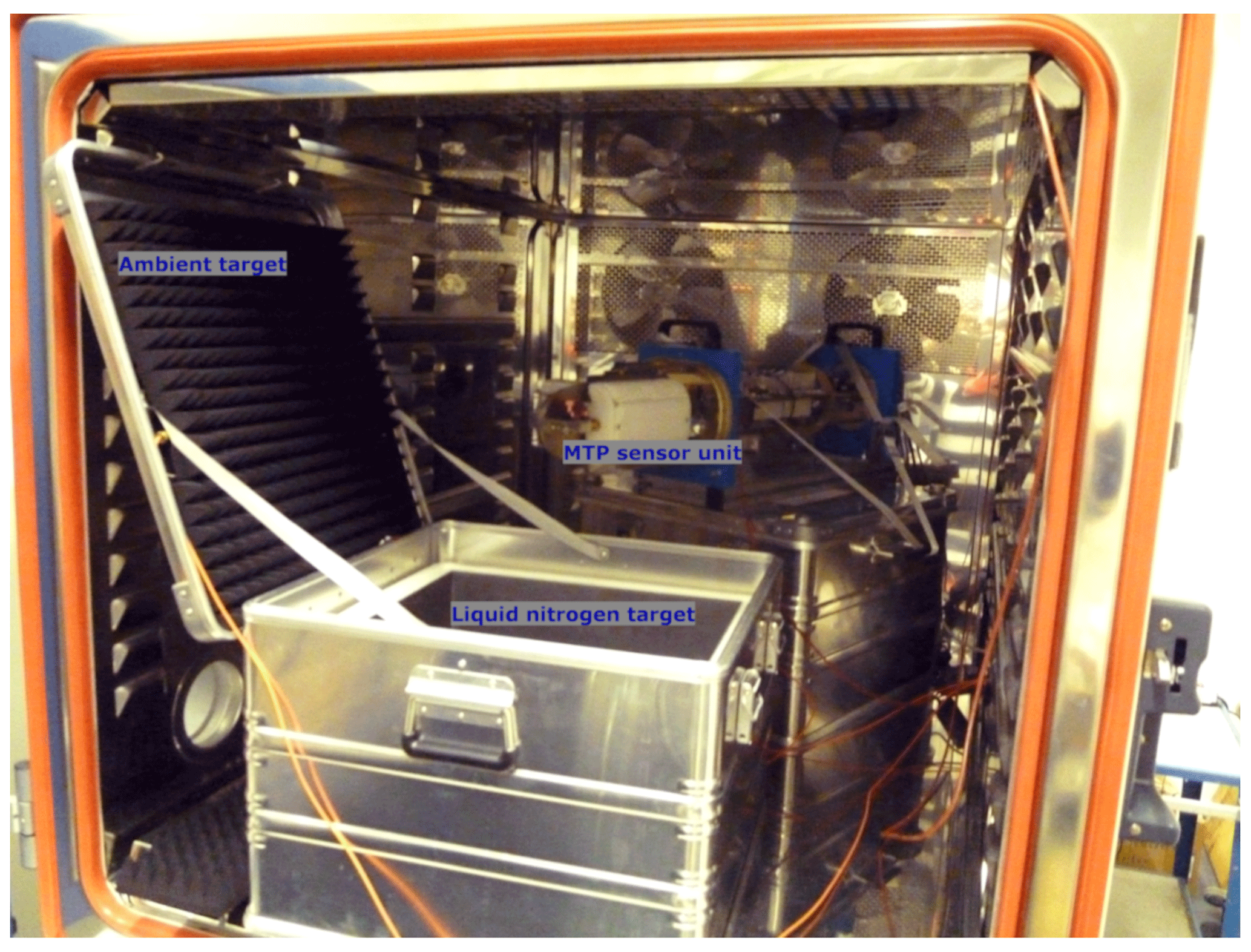
Figure 3 HALO MTP inside the cold chamber. For the measurements, the box containing the liquid nitrogen and the ambient target was rotated to face towards the MTP sensor unit. A second microwave absorber was placed on the ceiling of the chamber to function as a second ambient target.

Since this MTP instrument is mounted to the outside of the aircraft (see Fig. 1, left), the instrument experiences changes in surrounding pressure and temperature during measurement flights in which flight-level changes can be quite common. During a single mission flight, the air temperature surrounding the aircraft can change from around 300 K on the ground to as low as 190 K in the tropopause. These changing ambient temperatures of the MTP can influence the performance of the instrument: amplifiers might change their characteristics, and thus the relation between the recorded signal and the source temperature, i.e., the calibration parameters, change. Moreover, the noise diode used for calibration may change its signal strength (see Sect. 4.2), and the overall instrument noise can be affected. However, the noise characterization is particularly important when interpreting temperature fluctuations in a time series of MTP data. Knowing possible periodicity in the noise signal is essential to distinguish between real periodic atmospheric temperature fluctuations, e.g., those caused by gravity waves, and instrument noise. To test all of these characteristics, the MTP was placed inside a temperature chamber (Fig. 3) to simulate the changing outside air temperature during mission flights. In these tests, the influence of the changing surrounding temperature on the linearity of the sensor is tested (Sect. 3.2), and the measurements are used to determine the noise characteristics of the HALO MTP. The laboratory results are also compared to the noise characteristics derived from airborne ML CIRRUS mission data (Sect. 3.3). Possible calibration strategies and the effect of changing instrument state on the calibration of data will be discussed in Sect. 4.

3.1 Instrument function

The measurements of the instrument transmission functions, as well as of the antenna diagram, were made in a chamber completely covered in microwave absorbers. The MTP was installed on a rotatable platform. A tuneable signal source with a horn antenna was placed at 5 m of distance to the MTP instrument. The signal was then measured by the MTP and by a power meter for reference. The power of the source signal was chosen such that the MTP signal was well above its inherent noise level. For the measurement of the filter function, the source frequency was tuned between LO − 300 MHz and LO + 300 MHz in steps of 1 MHz. The measured signal is normalized and then corrected for frequency dependency based on the Friis transmission equation (e.g., Balanis, 1997):

$$\begin{array}{}\text{(2)}& {\mathrm{counts}}_{\mathrm{corr}}={\displaystyle \frac{{\mathrm{counts}}_{\mathrm{norm}}}{f^{\mathrm{2}}/{\left(min\left(f\right)\right)}^{\mathrm{2}}}}.\end{array}$$

Finally, the signal power of the source, P_corr(f), is taken into account in a final normalized signal representing the relative forward transmission, counts_final:

$$\begin{array}{}\text{(3)}& {\mathrm{counts}}_{\mathrm{final}}={\displaystyle \frac{{\mathrm{counts}}_{\mathrm{corr}}}{P_{\mathrm{corr}}\left(f\right)}}.\end{array}$$

The resulting instrument transmission functions for the three standard frequency channels are shown in Fig. 2a. It shows symmetrical shapes for all frequency channel functions (i.e., radiances are recorded symmetrically from both flanks of the probed oxygen line), confirming a transmission of the signal at ±200 MHz around the LO (the width of the plateau). The gap in the center is created by the receiver architecture using a double-side-band receiver as explained in Sect. 2. A certain “waviness” with an amplitude of about 0.5 dB is visible next to this gap. To exclude reflections from the chamber as a source, the measurements were repeated multiple times with slightly different positioning of the source antenna and the instrument. Since the results were similar in all measurements, the source of this waviness is attributed to some internal source within the instrument due to electromagnetic wave propagation through the instrument parts.

The main result of measuring the antenna diagram is the field of view (FOV) of the instrument, defined by the full-width half-maximum (FWHM; red dashed lines in Fig. 2b and c) of the antenna diagrams. It is actually mainly defined by the hyperbolic shape of the rotating mirror at the front of the instrument. The measurement was made using the same laboratory setup as for the measurement of the transmission function. Both the horizontal and the vertical plane were measured in steps of 1^∘ rotation. The symmetric shape of the diagram implies that radiance is picked up equally strong from all directions. Note that the maxima of the side lobes in the antenna diagrams have a maximum at −30 dB, meaning the signals from these spatial directions are 1000 times weaker than the signal picked up from the main viewing direction. The FOV is about 7.0–7.5^∘ in the horizontal and about 6.5–7.0^∘ in the vertical at all frequencies.

A spillover measurement of the horn antenna (as investigated, for example, in McGrath and Hewison, 2001) and a test of the stability of the LO frequency generator were not possible, as this would have required disassembling parts of the instrument, which was not an option at that time due to aircraft certification issues.

3.2 Temperature dependence of MTP characteristics

To investigate the temperature dependence of instrument performance, a series of measurements inside a cold chamber was performed (see Fig. 3). During this measurement series, the temperature of the cold chamber was successively lowered from 21 to −15 ^∘C in steps of 5 ^∘C. This temperature range resembles the temperatures the MTP experienced during its deployment in the ML CIRRUS campaign in 2014, as shown in Fig. 4b. The pod air temperature sensor monitors the temperature inside the MTP's housing during the flight (see Fig. 1b). In the cold chamber, the housing was not installed to prevent overheating of the instrument at higher temperatures. As a result, the readings of this sensor show the air temperature inside the cold chamber. The scanning unit temperature sensor keeps track of the temperature of the MTP instrument within close proximity to the crucial parts of the radiometer, such as the amplifiers and the mixer. The readings of this sensor give an impression of the state of the instrument and its thermal stability. It can be seen that the response to lowering the cold-chamber temperature is different between the two sensors. This is caused by the placement of the sensors, with one being closer to some heated parts of the instrument, indicating that changes in the environment of the instrument do not equally influence all parts of the instrument. Moreover, from the readings of the scanning unit temperature sensor (black line in Fig. 4a) it can be seen that the MTP instrument takes some time to stabilize under the new temperature conditions. This time required for stabilization depends a lot on the operating environment, such as the size of the laboratory space, ventilation, and ambient temperature. In this setting, it takes up to 15 min after the initial temperature change. Only those parts of the measurement series are used in which the scanning unit temperature is stable (the difference between two readings being smaller than an empirical threshold value of 0.04 K) to exclude effects from the instrument adjusting to new environmental conditions.

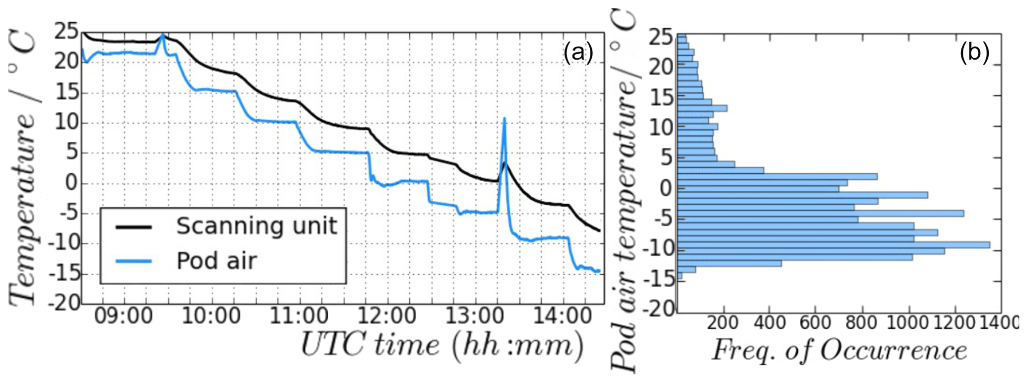
Figure 4 Temperature sensor measurements during cold-chamber measurements (a; black line: scanning unit sensor, blue line: pod air sensor). At 0 ^∘C (∼ 11:45 UTC) the cold-chamber software had to be restarted, causing a longer stabilization period, and at −5 ^∘C (∼ 13:15 UTC) the cold chamber was opened to refill the liquid nitrogen in the cold target, causing spikes in the temperature measurement. (b) Pod air temperature measurements during all ML CIRRUS campaign flights.

Along with the MTP instrument two microwave absorbers (Telemeter Electronic GmbH EPP51 broadband pyramidal absorber) at ambient temperature (hereafter referred to as “ambient targets”) and a similar microwave absorber submerged in liquid nitrogen (hereafter referred to as the “cold target”) were placed in the chamber in order to perform calibration measurements throughout the complete measurement series. The third type of calibration target used in this measurement series is the built-in calibration target of the MTP instrument (see Sect. 2), hereafter referred to as the “hot target”.

Linearity of the sensor

Using the measurements of the two ambient targets installed within the chamber, it can be shown that for the HALO MTP the linear relation between the source temperature and the measurement output is given at all standard frequency channels (see Fig. 5). Fits to the data using higher orders show that only the linear term significantly contributes to the data fit. Since the temperature of not only the target, but also the temperature of the sensor unit itself, changed during this test, which are both monitored (see Fig. 4), it can also be established that the linear relationship between the measured signal and the source temperature is maintained throughout changing conditions. The measurements corresponding to the two individual ambient targets (different line colors in Fig. 5) are nearly identical, proving the consistency of measurements.

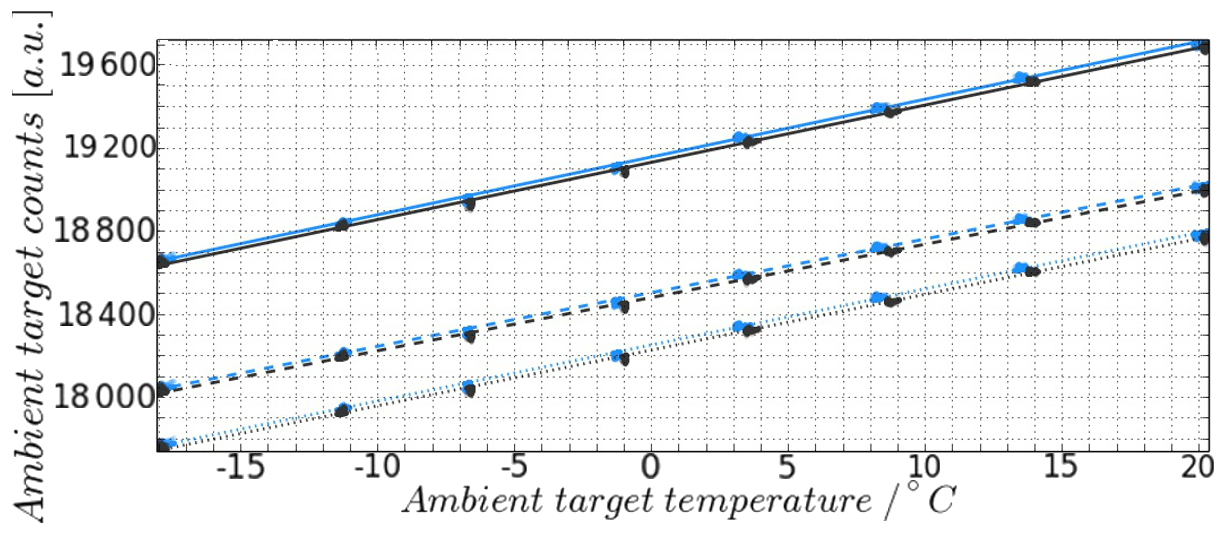
Figure 5 Ambient target temperature vs. the measured signal (counts) of the two ambient targets for all three standard frequency channels of the HALO MTP (different line styles). Different line colors correspond to the measurement of the two individual ambient targets.

The calibration parameters needed to calculate the brightness temperature (T_B) from the measured signal (“counts”; c) are therefore the y intercept (receiver noise temperature; T_R) and the slope of the line (s_cal) drawn through two points defined through measurements of calibration targets at known temperatures:

$$\begin{array}{}\text{(4)}& T_{\mathrm{B}}=c\cdot s_{\mathrm{cal}}-T_{\mathrm{R}}.\end{array}$$

In Sect. 4 it will be shown that those parameters depend on the instrument state and can be related to housekeeping data. Please note that in the classical microwave notation, the calibration is actually defined inversely as $T_{\mathrm{B}}=c\cdot G+T_{\mathrm{R}}$, in which the gain (G) is equal to the inverse slope as defined in the above equation.

3.3 Noise characterization

The instrument's noise was characterized using the signal measured when pointing towards the hot target. It is assumed that due to the temperature stabilization of the target, the mean measurement signal should not change over time. Hence, the deviation from the mean represents the noise added by the instrument. An example of the measured signal while looking at the hot target during one measurement segment at constant cold-chamber temperature is shown as the grey line in Fig. 6. Obviously, absolute stability can hardly be reached in a cold environment, while parts of the sensor unit are heated to approximately 40 ^∘C, which is taken into account by applying a linear fit to the measured data of one segment (black line in Fig. 6) instead of simply subtracting the mean (blue line in Fig. 6). Using all segments of the cold-chamber measurements, the resulting HALO MTP noise characteristics, as shown in Fig. 7 (top), can be described by a Gaussian distribution with a standard deviation of approximately 6 counts (approximately 0.25 K) and a mean of 0 counts.

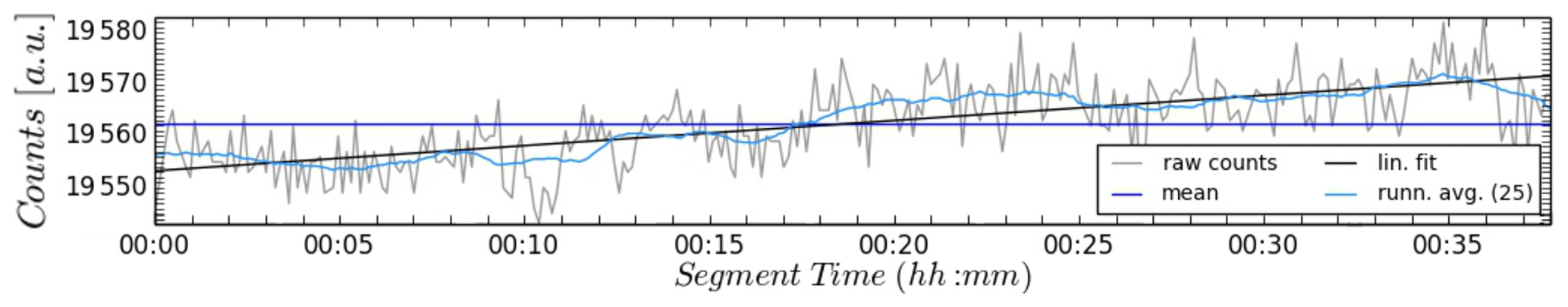
Figure 6 Measured signal (grey line) at 56.363 GHz while looking at the ambient target inside the cold chamber as well as a running average (light, blue line), mean value (blue line), and linear fit (black line). The corresponding brightness temperature change in the linear fit during the segment is about 0.8 K.

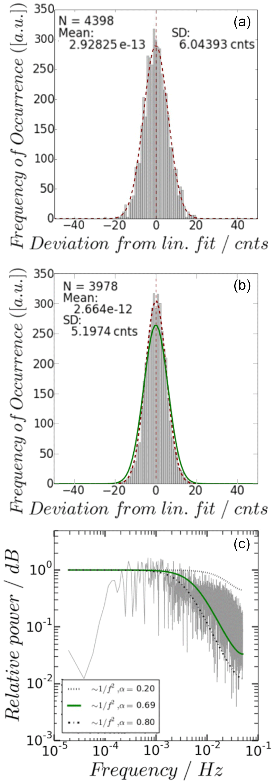
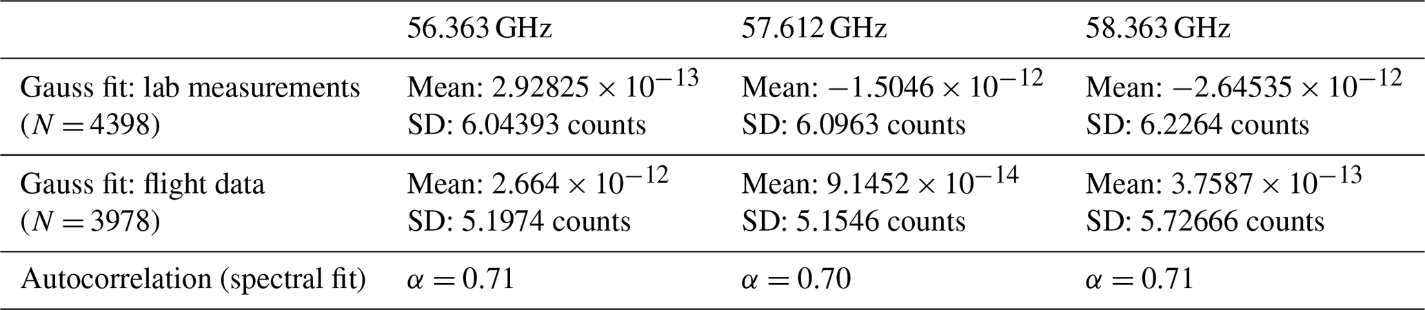
Figure 7 HALO MTP noise characteristics at 56.363 GHz. Figures for the other two standard frequency channels look similar. Fit parameters for all three frequency channels are summarized in Table 2. (a) Laboratory measurements in the cold chamber. Red dashed line: Gauss fit to the data. (b) Derived from ML CIRRUS flight data. Green line: ideal Gauss function with the mean at 0.0 and a standard deviation of 6 counts (∼ 0.25 K), as implied by the cold-chamber noise spectrum. (c) Noise spectrum calculated from ML CIRRUS flight data. Black dashed lines: theoretical power spectra of $\mathrm{1}/f^{\mathrm{2}}$ noise with lag-1 correlations of α=0.2 and α=0.8. Green solid line: theoretical power spectrum of $\mathrm{1}/f^{\mathrm{2}}$ noise with lag-1 correlation of input data.

The same method as for the cold-chamber measurements is used for HALO MTP data recorded during the ML CIRRUS campaign in 2014. Here, the criterion used to determine flight segments with nearly stable instrument states is a difference in the scanning unit temperature of less than 0.04 K between two measurement cycles. Additionally, it was ensured that no altitude changes were made (Δz≤25 m) and no curves were flown during these segments. From all ML CIRRUS mission and test flights, 61 segments could be identified that satisfied the criteria and were at least 5 min long to ensure significance of statistical results from the length of one segment: with the length of one measurement cycle (including a calibration measurement at the end) at 13 s each segment includes at least 22 recordings of the hot target measurement signal. Figure 7b shows the noise characteristics at 56.363 GHz. The results from the flight data evaluation are in excellent agreement with the values found in the laboratory environment, showing even smaller standard deviations of 5.2–5.7 counts, depending on the frequency channel. This is strong evidence that the HALO MTP noise characteristics do not change between flights, and laboratory assessment can be used to determine overall instrument health and comparability of measurements between campaigns, also serving as information for the retrieval development.

Table 2 HALO MTP instrument noise characteristics at each of the three standard frequency channels.

For the spectral analysis of the MTP measurement noise the 61 ML CIRRUS mission flight segments are used again. Due to the varying lengths of the individual flight legs, the data are concatenated to a single timeline for spectral analysis. The power spectrum of the noise signal of the HALO MTP at 56.363 GHz, as shown in Fig. 7 (bottom), reveals that the measurement noise can best be described as red noise, which is characterized by the autocorrelation α between a data point of the time series and its precursors. According to Torrence and Compo (1998), the corresponding theoretical noise power spectrum for a range of wave numbers k, P_k, is given by

$$\begin{array}{}\text{(5)}& P_k={\displaystyle \frac{\mathrm{1}-{\mathit{\alpha }}^{\mathrm{2}}}{\mathrm{1}+{\mathit{\alpha }}^{\mathrm{2}}-\mathrm{2}\mathit{\alpha }\cos (\mathrm{2}\mathit{\pi }k/N)}}.\end{array}$$

For the three standard frequency channels, the lag-1 autocorrelation of MTP measurements during the ML CIRRUS campaign is α≅0.7. Fit parameters characterizing the noise characteristics at the three standard frequency channels are summarized in Table 2.

With the above findings, characterizing the HALO MTP measurement noise as Gaussian-shaped, with a mean of 0 counts and a standard deviation of 6 counts, as well as with the knowledge of the inherent periodic structure of the noise signal, it is now possible to determine whether periodic structures in an MTP temperature measurement time series are significant (high probability that they result from atmospheric temperature fluctuations) or noise-induced. Additionally, the standard deviation of the Gaussian distribution of noise values can be used to determine the variance of TBs derived from the raw signals once the calibration parameters are known. While it would be interesting to investigate the integration time needed to significantly reduce the measurement noise (e.g., by applying the Allen variance), any increase in integration time will decrease the horizontal resolution of measurements taken on a jet-engine aircraft. The current settings present a well-chosen compromise between the measurement noise and the horizontal resolution of the MTP data (MJ Mahoney and Richard Denning, private communication, 2013). As the calibration measurement is already made at the end of each measurement cycle, the instrument is calibrated as frequently as possible, and the calibration performance cannot be further improved by adding more calibration measurements during mission flights.

4 Investigation of calibration methods for the HALO MTP

In Sect. 3.2 it was shown that there is a linear response in the measured signal to changes in the source temperature so that the measured signal can be related to a brightness temperature by using the linear relation in Eq. (4). While a line can be fitted through any two known points, which makes the calibration process very simple, the determination of the calibration parameters also faces the danger of inconsistencies under rapidly changing measurement conditions, which could lead to large errors in the calculated TBs. The cold-chamber measurements described in the previous section are used to investigate the influence of the changing instrument state (due to changing surrounding temperature) on the calibration parameters and the ND signal. To determine a best practice for calibration of MTP raw data, various methods to calibrate HALO MTP data are described in the following, giving a brief overview of their respective advantages and disadvantages in connection with the HALO MTP.

1. The first calibration method is hot–cold calibration with a cold target (microwave absorber submerged in liquid nitrogen) at temperature T_cold and an ambient target (microwave absorber at room temperature) at temperature T_amb to derive the calibration parameters. This is the standard calibration method of radiometers in a stable environment. Using this method to calibrate the sensor, before or after taking measurements in the atmosphere, provides the calibration parameters based on two temperatures which lie on the upper edge and below the expected measurement range. Thus, the validity of the calibration for the following measurements can be ensured, as long as the sensor itself is in the same surrounding conditions during the calibration as during the atmospheric measurements and sufficient instrument stability is given. Since this stability is not given for the MTP instrument, the equations applied for this calibration method are the following:

   $$\begin{array}{}\text{(6a)}& {\displaystyle }{T}_{\mathrm{B}}^{\mathrm{CCh}}\left(c\right)=s_{\mathrm{cal}}^{\mathrm{CCh}}\left(c_{\mathrm{hot}}\right)\cdot c-T_{\mathrm{R}}^{\mathrm{CCh}}\left(c_{\mathrm{hot}}\right),\text{(6b)}& {\displaystyle }{s}_{\mathrm{cal}}={\displaystyle \frac{T_{\mathrm{amb}}-T_{\mathrm{cold}}}{c_{\mathrm{amb}}-c_{\mathrm{cold}}}},\text{(6c)}& {\displaystyle }{T}_{\mathrm{R}}=T_{\mathrm{amb}}-s_{\mathrm{cal}}\cdot c_{\mathrm{amb}},\end{array}$$

   in which c_hot denotes a system parameter that describes the instrument state (see following section) so that in-flight data can be related to the cold-chamber laboratory measurements within a similar instrument state (indicated by the index CCh). Using the hot–cold calibration method is necessary to characterize the noise diode signal used in the second calibration method as described below. However, since it makes use of external calibration targets, the calibration measurement can only be performed on the ground, where single calibration measurements at arbitrary room temperatures may not be representative of the instrument state during flight, as shown below. However, this method can be used to check the overall health of the instrument between deployments.

2. The second calibration method is using the MTP built-in hot target (microwave absorber with a heated metal plate in the back) at temperature T_hot combined with a noise diode offset signal c_ND.

   $$\begin{array}{}\text{(7a)}& {\displaystyle }{T}_{\mathrm{B}}^{\mathrm{ND}}\left(c\right)=s_{\mathrm{cal}}\cdot c-\left(T_{\mathrm{hot}}-s_{\mathrm{cal}}\cdot c_{\mathrm{hot}}\right)\text{(7b)}& {\displaystyle }{s}_{\mathrm{cal}}={\displaystyle \frac{T_{\mathrm{ND}}}{c_{\mathrm{ND}}-c_{\mathrm{hot}}}}\end{array}$$

   This is the default way to calibrate MTP measurements. By using calibration measurements taken during flight, the calibration roughly follows the individual state of the instrument, whatever conditions the aircraft meets. The downside of this method is that a faulty noise diode signal can jeopardize reliable calibration. Also, in this method two reference temperatures are used, which are above the expected measurement range: the built-in calibration target is up to 100 K warmer than the outside air temperatures during flight, and T_ND is added to this temperature. Hence, small uncertainties in the determination of the calibration parameters may lead to large deviations in the calibrated data.

3. The third calibration method is using the MTP built-in hot target combined with HALO static temperature (HALO TS) using the equation

   $$\begin{array}{}\text{(8a)}& {\displaystyle }{T}_{\mathrm{B}}^{\mathrm{TS}}\left(c\right)=s_{\mathrm{cal}}\cdot c-\left(T_{\mathrm{hot}}-s_{\mathrm{cal}}\cdot c_{\mathrm{hot}}\right),\text{(8b)}& {\displaystyle }{s}_{\mathrm{cal}}={\displaystyle \frac{T_{\mathrm{hot}}-\mathrm{TS}}{c_{\mathrm{hot}}-c_{\mathrm{0}{}^{\circ }}}}.\end{array}$$

   Here, $c_{\mathrm{0}{}^{\circ }}$ represents the recorded signal at the horizontal viewing angle, which corresponds to the forward-looking measurement, probing the air masses directly in front of the aircraft. This method is an alternative to the previous calibration method in the case that the noise diode signal cannot be used. It also follows the individual state of the instrument during measurement flights, but since this method uses the HALO static temperature measurement, the MTP data are no longer independent from the aircraft measurements.

Other calibration methods, such as tipping curve calibration (e.g., Küchler et al., 2016; Han and Westwater, 2000), are not available for the DLR MTP because of the given instrument design (mainly antenna beam width) and potentially fast-changing atmospheric conditions due to the moving platform, influencing radiative transfer calculations needed in this approach and the need for an efficient measurement strategy.

In the following, the three methods described above are applied to calibrate MTP data from the cold-chamber measurements (see Sect. 3.2). First, the hot–cold calibration is used to investigate the temperature dependence of the calibration parameters themselves (Sect. 4.1); then, the other calibration methods, which are based on data recorded during mission flights (“in-flight calibration”), are assessed and temperature effects are again discussed (Sect. 4.2). In Sect. 4.3 the calibration methods are tested and compared to each other using measurements recorded during the ML CIRRUS campaign deployment. A discussion of measurement uncertainty and a summary of the results, leading to an assessment of a best practice for the calibration of HALO MTP data after a campaign, are given in Sect. 4.4.

4.1 Hot–cold calibration in a cold chamber

When performing cold target measurements, the interference with a standing wave present between the instrument's receiver hardware and the surface of the slowly evaporating liquid nitrogen (see also Sect. 4.1.1 in Küchler et al., 2016) was taken into account. As the HALO MTP is a total-power radiometer (Denning et al., 1989), the output voltage of the detector is proportional to the square of the incoming intensity (Ulaby et al., 1981; Woodhouse, 2005). Thus, the times with the least interference of the original signal and the standing waves are defined by minima in the measured signal time series. To find those minima in the cold-chamber measurement time series, several steps were taken: (i) a running average (N=25) is used to minimize the noise in the data; (ii) a spline fit is used to find a smooth curve, representing the measurements; (iii) the fit is used to interpolate to a higher time resolution; and (iv) the minima of this interpolated curve are used to identify those individual measurement cycles closest to the minima in the time series on which the calibration will be based. Due to noise, the calibration becomes more reliable if a mean of more than one measurement close to a minimum in the time series is used; hence, the five measurements closest to the time of a minimum in the smooth curve are always included in the analysis.

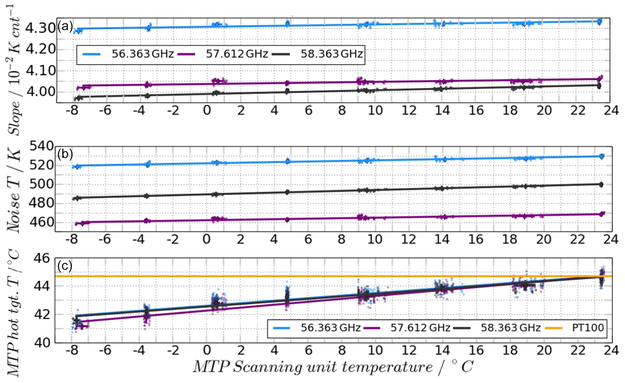
Figure 8 Calibration parameters calculated from hot–cold calibration for standard frequency channels during cold-chamber measurements. (a) Slope of calibration line. (b) Receiver noise temperature (T_R). (c) Calculated hot target TBs at different scanning unit temperatures during cold-chamber measurements. Small dots: single measurements contributing to the average at one scanning unit temperature. Orange line: Pt100 sensor readings.

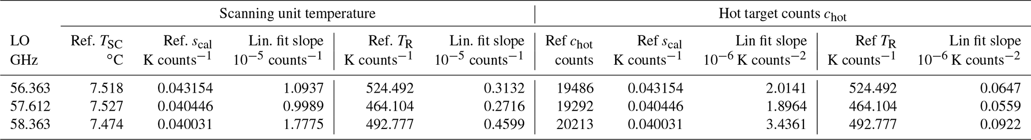
The resulting calibration parameters are plotted over the corresponding scanning unit temperatures at the time the minimum in the cold target measurements occurred. Figure 8 clearly shows that the parameters change with the scanning unit temperature. That corroborates the assumption that HALO MTP flight data cannot simply be calibrated by using fixed calibration parameters from laboratory measurements at single arbitrary room temperatures, since such measurements are only representative of specific instrument states. Still, it is possible to apply a linear fit to the data by providing a relationship between the MTP scanning unit temperature and the calibration parameters to be used at these temperatures. The same is true when using the hot target measurement signal as a reference, which might better represent the current state of the instrument than the scanning unit temperature. The linear fit parameters are summarized in Table 3.

Table 3 Linear fit values linking calibration slope values and receiver noise temperature T_R (calibration y intercept) to MTP scanning unit temperature and hot target counts.

4.2 Calibration using the MTP built-in target

When applying this (default) calibration method to MTP data, everything builds on the following two assumptions: (i) the ND offset signal is the same each time the calibration measurements are performed, and (ii) the TB measured when pointing towards the heated target corresponds to the measurements of the temperature sensors at the back of the target. Both assumptions are tested in the following using the calibration measurements performed in the cold chamber.

4.2.1 Noise diode offset temperature

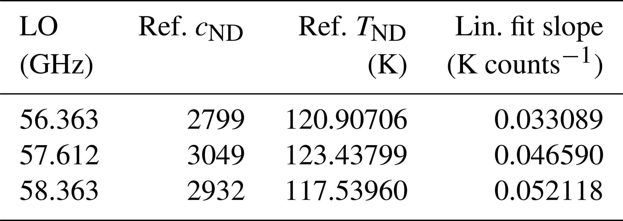
The ND offset signal is characterized using the hot–cold calibration method used during the cold-chamber measurement series, during which the ND is repeatedly activated. Since the calibration parameters are already known from the hot–cold calibration, the temperature offset connected to the signal offset created by the ND can be calculated. Resulting HALO MTP ND offset temperatures are shown in Fig. 9. The ND offset temperature obviously depends on the count offset resulting from the induced noise in the input signal, which shows a clear dependency on the sensor unit temperature (coloring of the dots in Fig. 9). Again, it is possible to apply a linear fit between the recorded ND offset signal, ${\widehat{c}}_{\mathrm{ND}}=c_{\mathrm{ND}}-c_{\mathrm{hot}}$, and the associated ND offset temperature derived from the hot–cold calibration method. This fit can be used to find the correct ND offset temperature required in the calibration of mission data. The linear fit values of this correction are shown in Table 4 (last column). In Fig. 9 the deviation of noise diode counts from the linear fit can be as large as 20 counts (approximately 0.83 K) for any of the three frequency channels. This spread translates into the remaining uncertainty in the ND offset temperature.

Figure 9 Calculated ND offset temperature for occurring ND count offsets (for better comparability, the means of the temperature and count values have been removed – mean values are shown in Table 4). Color coding is as follows. For the MTP scanning unit temperature blue indicates colder and red warmer; black line: linear fit linking ND offset temperature to offset counts.

Table 4 Linear fit values linking the noise diode offset temperature to MTP noise diode offset counts.

4.2.2 Calibration based on outside air temperature

During its deployment in the ML CIRRUS campaign in 2014, occasional failures of the ND, caused by a faulty soldered joint, were experienced. As the ND signal could not be used for calibration, HALO TS can be used instead. This temperature is interpreted as the TB measured at 0^∘ elevation (horizontal measurement). Simple radiative transfer calculations show that the MTP measurements at all standard frequency channels are most sensitive to the air directly in front of the sensor (less than 2 km of distance; see Appendix or Kenntner, 2018, for more details). Thus, the average HALO TS value of the 13 s period it takes to record an entire MTP measurement cycle (with the 0^∘ measurement being in the middle of the cycle) is representative of the air masses probed by the 0^∘ elevation measurements. Hence, the calibration parameters can also be derived by combining the calibration measurement while pointing at the hot target with the horizontal measurement using Eq. (8a).

4.2.3 Hot target temperature measurement

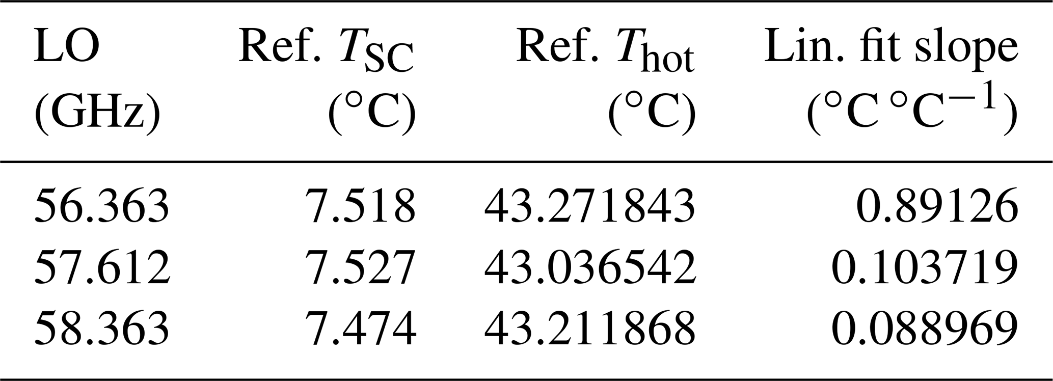
The housekeeping data of the MTP indicate large temperature differences of up to 55 K between the air in front of the hot target and the heated back. Temperature gradients within the absorber material could lead to a misinterpretation of the measured brightness temperature, since the calibration measurement is mostly influenced by the front of the absorber, the exact temperature of which is unknown. There are no temperature sensors built into the absorber material, which could be used to derive the thermal gradient, and measurements with a thermal imager would require disassembling of the instrument and are not an option. Still, to investigate the hot target measurement characteristics, the calibration parameters determined from the hot–cold calibration method are used to calculate the hot target TB associated with the current measurement signal. Indeed, Fig. 8c shows the clear trend towards colder TBs with lower scanning unit temperatures, which correspond to a colder environment of the MTP instrument, contrary to the readings of two Pt100 temperature sensors, which show the intended target temperature of the heaters placed at the metal back of the target of just below 45 ^∘C during entire mission flights (orange line in Fig. 8c). The difference can be as large as 3 K. However, the linearity of the sensor again allows for a linear fit between the current scanning unit temperature and the average associated hot target TB. Thus, in-flight calibration can be performed using a corrected hot target TB, according to the MTP instrument's housekeeping data. The parameters to correct the hot target TBs used in the calibration are shown in Table 5.

Table 5 Linear fit values used to correct the MTP hot target brightness temperature.

4.3 Comparison of calibration methods

There are eight different ways to perform the calibration calculations with and without applying the corrections discussed in the previous sections, as summarized in Table 6. All methods are compared to find the best practice of deriving TBs from MTP raw counts by applying all eight methods to the same set of mission data. To do so, segments from all ML CIRRUS mission flights are used during which the altitude of the aircraft did not change by more than 50 m during a measurement cycle and no curves were flown (roll smaller than 5^∘). Note that this definition of usable segments is not based on any parameters connected to the instrument state of the HALO MTP (e.g., scanning unit temperature), leading to the inclusion of measurement cycles with possibly unstable measurement conditions, e.g., shortly after altitude changes. The only exception is that only those segments are used, during which the ND did not show failures, to ensure comparability of all calibration methods. This way, 38 flight segments with at least a 10 min duration (i.e., including at least 50 measurement cycles) could be identified. The TBs are calculated based on each individual measurement cycle, but using the calibration coefficients (s_cal and T_R) calculated from the average of the relevant data from the seven previous cycles, the seven following cycles, and the cycle itself (N = 15) to account for noise in the calibration measurement signals. As an example, the resulting TBs of the 56.363 GHz measurements at a 0^∘ limb-viewing angle during one segment of ML CIRRUS flight MLC10 on 11 April 2014 are shown in Fig. 10 (top panel). The TBs resulting from all calibration methods show the same time-dependent variations and mainly differ in their offset to HALO TS, indicating that differences in the respective calibration coefficients affect the absolute accuracy of the derived TBs more than the precision.

Table 6 Calibration methods tested with MTP data. T_SC indicates linking of the parameters to the scanning unit temperature, and c_hot indicates linking to the hot target measurement signal. Usage of uncorrected data is denoted with a (u), and applied corrections are indicated with a (c).

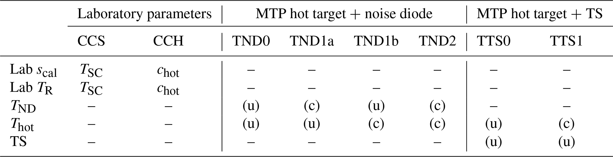
Figure 10 Top panel: difference between HALO static temperature and TBs derived with the eight calibration methods defined in Table 6 derived from the horizontal measurements at 56.363 GHz during one segment of an ML CIRRUS mission flight. Lower part: same as the top, but plotted relative to method TTS1 and with an applied offset correction at six different elevation angles measured at 56.363 GHz. Red crosses in lower left panel: difference between method TTS1 and HALO TS. Refer to Table 6 for the denomination of the calibration methods.

To further investigate the precision of the MTP measurements, a leg-mean value of the HALO TS and the TBs of the 0^∘ elevation measurements is used to determine the offset, which is subtracted from the TBs at all elevation angles:

$$\begin{array}{}\text{(9)}& T_{\mathrm{B}}^{\mathrm{corr}}\left({\mathit{\nu }}_{\mathrm{LO}},\mathit{\alpha }\right)=T_{\mathrm{B}}\left({\mathit{\nu }}_{\mathrm{LO}},\mathit{\alpha }\right)-\left(\stackrel{\mathrm{‾}}{T_{\mathrm{B}}\left({\mathit{\nu }}_{\mathrm{LO}},\mathrm{0}{}^{\circ }\right)}-\stackrel{\mathrm{‾}}{\mathrm{TS}}\right),\end{array}$$

with T_B(ν_LO,α) and $T_{\mathrm{B}}^{\mathrm{corr}}\left({\mathit{\nu }}_{\mathrm{LO}},\mathit{\alpha }\right)$ denoting the original and the corrected TBs under elevation angle α and at a specific frequency channel (i.e., LO), respectively. $\stackrel{\mathrm{‾}}{T_{\mathrm{B}}\left({\mathit{\nu }}_{\mathrm{LO}},\mathrm{0}{}^{\circ }\right)}$ denotes the leg mean of the original TBs measured under 0^∘ elevation, and $\stackrel{\mathrm{‾}}{\mathrm{TS}}$ represents the leg-mean HALO TS. By using leg-mean values to determine the offset, the corrected TBs will still contain individual small-scale structures, which might differ from those in the HALO TS measurements. Furthermore, large-scale trends of the background atmospheric temperature are also conserved in the resulting data. For individual calibration strategies, the subtracted offset can be as small as 0.8 K or as large as 7 K (see Fig. 10, top panel). The good agreement between all eight corrected TBs under the different viewing angles (see Fig. 10, lower part) indicates that removing the offset will not significantly change the shape of the temperature profile calculated in the retrieval. Moreover, the absolute accuracy of brightness temperature measurements now matches that of the HALO TS, which has an overall error of 0.5 K (Ungermann et al., 2015).

Figure 11 The rms difference between HALO TS and TBs derived from the MTP measurement signal at a limb-viewing angle of 0^∘ at the three standard frequency channels during all ML CIRRUS flight segments with no altitude changes, curves, or ND failures with signals longer than 10 min. Refer to Table 6 for the denominations of the calibration methods.

After applying the offset correction, the root mean square (rms) difference between the 0^∘ TBs and HALO TS, as shown in Fig. 11, gives a good impression of the capabilities of the different calibration strategies. Naturally, the methods that make use of HALO TS show the smallest deviation from HALO TS readings. However, it is the intention to maintain an independence of the MTP measurements from other measurement systems, increasing the value that MTP data add to the package of instruments flown on HALO. Of those calibration methods that do not use the HALO TS, the most reliable results are obtained when applying the method CCH, which uses the calibration values from the hot–cold calibration in the cold-chamber measurements related to the current hot target measurement signal. Whenever reliable ND measurements are available, this calibration method provides equally reliable results. Applying the corrections to T_ND or T_hot does not significantly change the result, but slightly smaller deviations from HALO TS are seen for the TBs derived using only the T_hot correction (method TND1b) and both corrections (method TND2). Considering the ND failures during the ML CIRRUS campaign, the favored calibration strategy is method CCH, also applying the offset correction between the leg-mean 0^∘ TB and the leg-mean HALO TS. The deviation between the resulting 0^∘ elevation TBs and HALO TS is ≤ 0.38 K at all three frequency channels for all ML CIRRUS flight legs with stable instrument conditions. This value is only exceeded when using the calibration method CCS – for all other methods it can be interpreted as the precision of MTP brightness temperature measurements, as will be shown below.

4.4 Discussion of HALO MTP measurement uncertainty

The overall uncertainty of the MTP measurements includes both systematic errors (e.g., the bias described above), and random errors (e.g., noise). In the case of the HALO MTP, the former can be related to HALO TS, as shown above, and the latter mainly influences measurement precision and the ability of the instrument to pick up atmospheric temperature fluctuations. In the literature (e.g., Ulaby et al., 1981), the standard formula to derive radiometric sensitivity (corresponding to the measurement precision of an ideal radiometer) is defined as the minimum detectable change in the radiometric antenna temperature of the observed scene:

$$\begin{array}{}\text{(10)}& \mathrm{\Delta }{T}_{\mathrm{theo}}={\displaystyle \frac{T_{\mathrm{sys}}}{\sqrt{\mathrm{\Delta }f\cdot \mathit{\tau }}}}={\displaystyle \frac{T_{\mathrm{R}}+T_{\mathrm{atmo}}}{\sqrt{\mathrm{\Delta }f\cdot \mathit{\tau }}}},\end{array}$$

in which Δf denotes the filter bandwidth, and τ represents the integration. The HALO MTP has an ideal filter width of Δf=200 MHz (see Fig. 2a) and uses an integration time of 200 ms. Assuming a receiver noise temperature of 493.79 K (see Table 7) and a mean atmospheric temperature of 250 K, this leads to a theoretical value of ΔT_theo=0.117 K. However, these values used to derive the theoretical value do not take into account gain fluctuations or the fact that the effective filter bandwidth is smaller than the ideal value due to small deviations depending on frequency and because of the gap in the center of the transmission function (see Fig. 2), so larger errors are expected for a real measurement system.

Table 7 Individual uncertainties of values used in brightness temperature calculation.

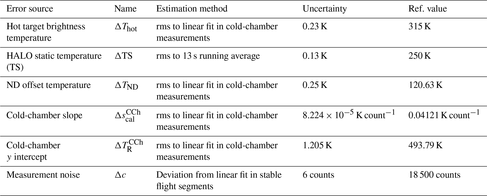
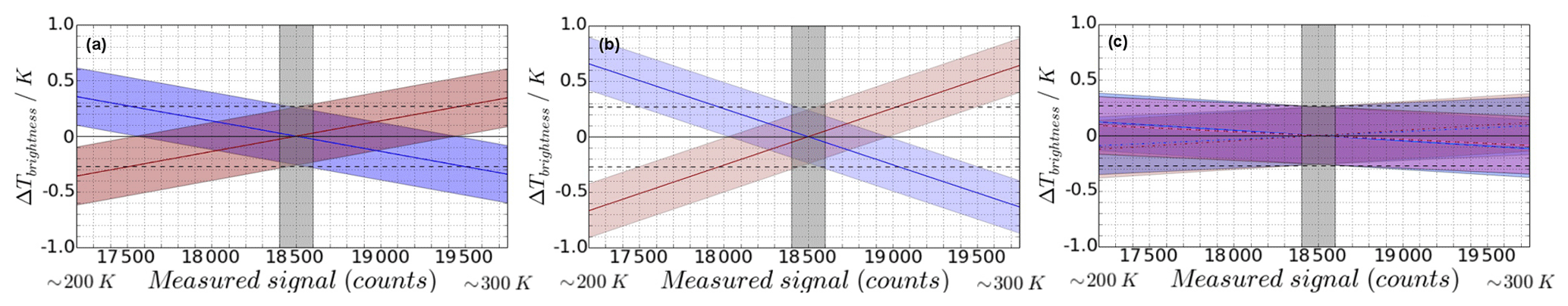
Figure 12 Error estimation of calibration methods with the applied HALO TS (assumed to be at 250 K) offset correction for the calibration methods (a) noise diode + hot target, (b) hot target + HALO TS, and (c) using cold-chamber calibration parameters. The measurement error for an individual measurement is indicated by the uppermost and lowermost edges of the blue or red shaded region (caused by measurement noise). Vertical grey shaded region: expected range of measurement signals if the 0^∘ measurement signal is at 18 500 counts (≈ 250 K). Black dashed horizontal lines: expected error induced by measurement noise of 6 counts.

In the calibration process, the main uncertainties arise from the use of the different reference temperatures, as summarized in Table 7. It is clear that the individual uncertainties assigned to each of the contributing values are not all independent. For example, the uncertainty of the y intercept (T_R) directly follows from the uncertainty of the slope of the line, but it is also directly influenced by the changing instrument state. Hence, a quadratic sum of the individual errors is not suitable and can lead to a large overestimation of the total TB error. Thus, a sensitivity analysis to estimate the overall measurement uncertainty is performed: reference values (see last column in Table 7) for all parameters with uncertainties are used in a reference calculation. With these values, TBs are calculated for a range of counts between 17 500 and 19 725, which corresponds to the measurement signal range for atmospheric temperatures, as seen during the ML CIRRUS campaign (approximately 200–300 K). Two control calculations are made, adding the corresponding individual uncertainties (see column 4 in Table 7) in a way that the slope of the calibration line becomes as steep as possible ($s_{\mathrm{cal}}^{max}$, red lines in Fig. 12) or as flat as possible ($s_{\mathrm{cal}}^{min}$, blue lines in Fig. 12), following

$$\begin{array}{}\text{(11a)}& {\displaystyle }{s}_{\mathrm{cal}}^{max}={\displaystyle \frac{\left(T_{\mathrm{1}}+\mathrm{\Delta }{T}_{\mathrm{1}}\right)-\left(T_{\mathrm{2}}-\mathrm{\Delta }{T}_{\mathrm{2}}\right)}{\left(c_{\mathrm{1}}-c_{\mathrm{2}}\right)-\mathrm{2}\mathrm{\Delta }c}},\text{(11b)}& {\displaystyle }{T}_{\mathrm{R}}^{max}=\left(T_{\mathrm{2}}-\mathrm{\Delta }{T}_{\mathrm{2}}\right)-s_{\mathrm{cal}}^{max}\cdot \left(c_s+\mathrm{\Delta }c\right)\end{array}$$

$$\begin{array}{}\text{(12a)}& {\displaystyle }{s}_{\mathrm{cal}}^{min}={\displaystyle \frac{\left(T_{\mathrm{1}}-\mathrm{\Delta }{T}_{\mathrm{1}}\right)-\left(T_{\mathrm{2}}+\mathrm{\Delta }{T}_{\mathrm{2}}\right)}{\left(c_{\mathrm{1}}-c_{\mathrm{2}}\right)+\mathrm{2}\mathrm{\Delta }c}},\text{(12b)}& {\displaystyle }{T}_{\mathrm{R}}^{min}=\left(T_{\mathrm{2}}+\mathrm{\Delta }{T}_{\mathrm{2}}\right)-s_{\mathrm{cal}}^{min}\cdot \left(c_s-\mathrm{\Delta }c\right),\end{array}$$

assuming that T₁ (with associated measurement signal c₁) is the warmer temperature used in the calibration. Comparing the TBs of the reference calculation to those of the two control calculations reveals the maximum uncertainty in the derived TBs.

Furthermore, in parallel to the offset correction introduced in the previous section, a TB correction for the control calculations is introduced: here, the offset correction is calculated from the difference between the TBs of the control calculation ($T_{\mathrm{B}}^{\mathrm{ctr}}$) and that of the reference calculation ($T_{\mathrm{B}}^{\mathrm{ref}}$) at 18 500 counts (∼ 250 K):

$$\begin{array}{}\text{(13)}& T_{\mathrm{B}}^{\mathrm{corr}}\left(c\right)=T_{\mathrm{B}}^{\mathrm{ctr}}\left(c\right)-\left(T_{\mathrm{B}}^{\mathrm{ctr}}\left(\mathrm{18}\mathrm{500}\right)-T_{\mathrm{B}}^{\mathrm{ref}}\left(\mathrm{18}\mathrm{500}\right)\right).\end{array}$$

Results for all three calibration methods are shown in Fig. 12. Within the typical region of measurements of one set of elevation angles (vertical grey shaded region in Fig. 12), the resulting uncertainty is comparable to or smaller than the expected error from the measurement noise itself ($\mathrm{\Delta }{T}_{\mathrm{B}}=\mathrm{\Delta }c\cdot s_{\mathrm{cal}}^{\mathrm{ref}}-T_{\mathrm{Sys}}^{\mathrm{ref}}$), indicated by the horizontal black dashed lines. The three approaches to calibrate MTP measurements produce comparable uncertainties in the derived TBs. However, the calibration method relating to the cold-chamber measurements is the most reliable in the case that the measured signals at certain viewing directions deviate largely from the measurement signal at the horizontal elevation (i.e., if large vertical temperature gradients are present around the current flight level). For all methods, the overall uncertainty is clearly below the already established value of ∼ 0.38 K mainly caused by the measurement noise. This is approximately 3 times larger than the theoretical value, which is expected, as the theory does not consider gain fluctuations (Ulaby et al., 1981). This is not representative of any real radiometric system that is applied outside controlled laboratory conditions, especially the MTP. It also confirms that the uncertainty of derived TBs is dominated by gain fluctuations. Any change in the measurement settings to use larger integration times, and thus reduce this noise, would be at the cost of horizontal resolution.

5 Further considerations relevant for retrieval setups

While this work excludes explicit retrieval studies, this section will provide brief insights into a few factors impacting retrieval outputs, which have not yet been mentioned. This includes further sources of input uncertainties and some considerations of how different measurement settings would impact the output quality.

5.1 Uncertainty from pointing error

The position of the HALO MTP instrument underneath the wing of the aircraft makes it sensitive to the altitude and speed of the aircraft. The bending and torsion of the aircraft body parts lead to deviations between the assumed pointing of the instrument and its true viewing direction. Adding to this is the aircraft pitch, which also depends on aircraft altitude and speed, introducing a potential source of a systematic error. During flights, the measurement of the inertial sensor, which is part of the HALO MTP that constantly records the current pitch angle of the instrument, is disturbed by the electromagnetic signal caused by the nearby mounted stepper motor, making the data not reliable enough to allow for a real-time correction of the pointing of the MTP instrument. Thus, the real pointing has to be determined after the flight. Analyzing the few reliable data points available after the two campaign deployments revealed that the relative deviation from the true horizontal plane was less than 1–2^∘ during entire mission flights. Compared to this, the MTP's FOV of 7–7.5^∘ (see Fig. 2 and Sect. 3.1) is clearly larger. Thus, it is safe to assume that a deviation of the elevation angle of 1–2^∘ from the assumed angle does not have a considerable influence on the uncertainty of the retrieval input.

5.2 Synthesizer errors

Another error source, which could not be studied in the lab, is a possible shift of the LO frequency. To measure the stability of the LO frequency generated by the synthesizer, it would be necessary to disassemble the instrument, which has serious implications for the certification of flying it on the aircraft. However, because of the placement of the LO frequency in the line center, a small shift will not create serious changes in the recorded TB; however, the measured TB would be caused by a slightly different altitude layer than expected. Because the strongest absorption lines of the absorption band are used, a notable effect would only be seen if the LO frequency shifted so much that one of the flanks of the line moved out of the filter range (in which case the overall health of the instrument should be checked). The effect is also dependent on the aircraft altitude, at which the error occurs due to the effect of line broadening. Furthermore, there is already a smearing effect caused by the FOV of the antenna, which dominates the altitude error, as long as the synthesizer error is small. Further investigation would certainly be useful in the retrieval setup using forward radiative transfer modeling.

5.3 Measurement settings impacting the retrieval output

There are several settings that can be easily changed when deciding the measurement strategy of the instrument. Both the set of elevation angles and the number and location of frequency channels used in a measurement cycle can be freely chosen. Simple geometric calculations, considering the length of the light path through an altitude layer, lead to a smaller set of elevation angles, which reduces redundancy between measurements due to the field of view of the instrument. Details can be found in the Appendix.

The frequency of the LO can be set between 48 and 64 GHz (see Table 1). Hence, there are quite a few possibilities to choose different frequency channels, including some at weaker absorption lines than in the standard setup. Using those, the instrument is able to view deeper into the atmosphere. As a reference, the MTP flown on the ER-2 research aircraft at ∼ 20 km of altitude only has a measurement range of approximately 2–3 km around flight altitude while using two frequency channels at similarly strong absorption lines to the current instrument (i.e., 57.3 and 58.8 GHz; Gary, 1989). Likewise, the height range of the DC-8 instrument, with LOs at 55.51, 56.66, and 58.79 GHz, has an “applicable range” (within which the weighting function drops to $\mathrm{1}/e$; see Appendix) of roughly ±2.8 km (Gary, 2006). In their conclusion on NCAR MTP data analysis Davis et al. (2014) mention that “it appears that more than about 3 km below the aircraft, the MTP may have difficulty identifying subtle mesoscale variations of temperature”.

The choice of frequency channels can have consequences on the calibration options but can lead to a clearly enhanced altitude range of sensitivity of the MTP. A pencil-beam calculation of the weighting functions at different frequency channels and viewing angles shows that changing the measurement strategy to include four frequency channels (instead of three) and only eight viewing angles (instead of 10) can significantly increase the vertical range and resolution of MTP measurements while still maintaining the length of one measurement cycle (i.e., not changing the horizontal resolution). However, an in-depth assessment of alternative measurement strategies must include forward radiative transfer modeling, using the information given in Sect. 3, and would go beyond the scope of this study. Details of the pencil-beam radiative transfer calculations and some implications for the calibration strategy are shown in the Appendix.

6 Summary

This study shows a thorough investigation of the MTP instrument operated by DLR and flown on the HALO aircraft. It is the first time a thorough characterization of an MTP instrument, including the assessment of brightness temperature calibration, has been published. Knowledge of the instrument characteristics, such as the instrument transmission function, the antenna diagram, its calibration, related measurement uncertainties, and the vertical observation range, is fundamental to the correct setup of a retrieval algorithm and for the interpretation of the retrieved temperature signals and conclusions about the atmospheric conditions around flight altitude.

Using the standard measurement settings, the instrument response function was determined along with the antenna diagram (Sect. 3). The results show symmetric shapes of all transmission functions, which is the desired and expected result. While small side lobes are detected in the antenna diagram, the main lobe has a symmetrical Gaussian shape, with a full-width half-maximum of 7.0–7.5^∘, which represents the field of view of the instrument. A smaller field of view could only be achieved by using a different shape of the rotating mirror and a larger horn antenna, which the compact design needed for the wing-carrier instrument does not allow for.

Measurements in a cold-chamber setup, as well as data recoded during a field campaign, were used to characterize the MTP's noise (Sect. 3). It can be described by a Gaussian distribution with a mean of 0 counts and a standard deviation of 6 counts (slightly less than 0.25 K). It was shown that the measurement noise can be characterized as red noise with a lag-1 autocorrelation of 0.7, which indicates that a time series of MTP data may show wave-like structures caused by internal noise; however, the presented characterization of the HALO MTP noise allows the identification of significant atmospheric signals in MTP measurement time series, as long as the amplitude of the atmospheric signal is larger than the measurement precision (i.e., significantly larger than 0.38 K), and wave-like signals (e.g., caused by gravity waves) can be clearly separated from the noise-induced structures caused by the autocorrelation of MTP measurements.

Furthermore, in the laboratory measurements the linear relationship between the instrument's measurements and the source temperature could be confirmed. Based on this linear relationship, the calibration of MTP raw data to derive brightness temperatures is possible and was further analyzed (Sect. 4). The measurements revealed clear changes in all calibration parameters, depending on the cold-chamber temperature. This includes a change in the measured brightness temperature when pointing towards the built-in hot calibration target, a change in receiver noise temperature caused by the electrical parts, and a change in the calibration slope caused by a change in amplification of the signal. Corrections to account for those changes have been found, and it could be shown that with the application of those corrections, brightness temperatures could be derived from ML CIRRUS mission data with an accuracy matching that of the HALO static temperature and a precision better than 0.38 K. The necessity of an offset correction relative to HALO TS has been identified for both the calibration relating to laboratory measurements and using the noise diode signal. The correction procedure was introduced as comparing the leg mean of the calculated TBs at 0^∘ elevation angle (horizontal measurement) to the leg mean of HALO TS. While removing a potential bias on the measured brightness temperatures, this method conserves trends in the background atmospheric temperature, as frequently observed during longer flight legs.

It was shown that all presented calibration methods produce comparable results. Considering the desire for MTP measurements mostly independent from other measurements (such as the HALO TS, which can then be used as a reference) and technical problems with the ND experienced during the ML CIRRUS campaign in 2014, the favored method of calibration is to use calibration parameters from the cold-chamber measurement series linked to the system state via the measurement signal while pointing towards the MTP built-in target. When analyzing the uncertainty of the calibrated brightness temperatures (Sect. 4.4), it was found that this method performs best whenever large vertical temperature gradients are present near flight level. Furthermore, the analysis of the uncertainties of the calibration parameters shows that they are clearly dominated by the contribution from measurement noise. Other uncertainties, such as the pointing of the instrument and synthesizer errors, are negligible compared to this uncertainty.

A brief discussion has been given on possibilities to further improve the quality and value of MTP measurements (Sect. 5) by changing the measurement setup within the given possibilities allowed by the instrument hardware. Simple estimations indicate that the signal is mostly influenced by the first 1.5–2 km of distance to the aircraft altitude both above and below flight level. The instrument hardly collects any usable information on the state of the atmosphere outside the resulting ∼ 3 km region around flight altitude (i.e., ±1.5 km around flight level). A proposal to improve the measurement strategy for future missions of the MTP is made, involving a reduction of the number of elevation angles used and including frequencies of weaker absorption lines of the 60 GHz oxygen absorption complex. The considerations shown in the Appendix indicate that the range of sensitivity above the aircraft can be increased to at least 2 km and up to approximately 4–5 km below the aircraft at an aircraft altitude of 11 km. At the same time, the horizontal resolution of MTP measurements can be maintained. This is a significant improvement in the value of MTP data.

Overall, this study summarizes the investigation of instrument parameters and characteristics necessary to accurately analyze and interpret the data produced by HALO MTP measurements. It is the basis to understand measurement uncertainty and the (vertical) range in which derived atmospheric properties are valid, to identify significant atmospheric signals in times series of HALO MTP data, and to act as a guideline for choosing the best possible strategy to record and calibrate mission data. Using this information, the best possible data input for the retrieval algorithm used to derive absolute temperature profiles can be obtained. With that basis the HALO MTP can provide valuable information on the atmospheric state, which can be utilized in many studies on atmospheric dynamics or in connection to in situ and other remote sensing measurements made on the same mission flights.

Appendix A: Simple approaches to increase the range of sensitivity

The altitude range of sensitivity and the vertical resolution of the retrieved temperature profile from MTP data depend on the set of frequency channels and the set of elevation angles used when recording MTP data, respectively. For an in-depth test of the optimal settings a full retrieval feasibility study would be mandatory, which is beyond the scope of this study. In the following the results of idealized radiative transfer (RT) simulations (cloud-free, not considering any special cases) are summarized to demonstrate the impact of these settings.

For this assessment the transmission and weighting functions (e.g., Ulaby et al., 1981) are of central importance. Transmission, $T\left(\mathit{\nu }\right)=\exp (-\mathit{\tau }(\mathit{\nu }\left)\right)$, characterizes the ratio of outgoing to incoming radiation traversing an atmospheric layer with path coordinate s. It is expressed through the optical depth τ(ν) defined as the integral of the absorption coefficient (α), which depends on the frequency (ν), the (path-dependent) atmospheric pressure (p(s)), and temperature (T(s)) of the layer within the plane-parallel atmosphere:

$$\begin{array}{}\text{(A1)}& \mathit{\tau }\left(\mathit{\nu }\right)=\underset{\mathrm{0}}{\overset{s}{\int }}\mathit{\alpha }\left(\mathit{\nu },p\left(s^{\prime }\right),T\left(s^{\prime }\right)\right)\mathrm{d}{s}^{\prime }.\end{array}$$

For brevity, in the following, the path dependency of α is expressed as α(ν,s). To investigate the range of sensitivity it is useful to calculate the signal contribution from each respective layer of the atmosphere, determined by the weighting function (WF) defined as

$$\begin{array}{}\text{(A2)}& \begin{array}{rl}W\left(\mathit{\nu },s\right)& ={\displaystyle \frac{\partial T(\mathit{\nu },s)}{\partial s}}=\mathit{\alpha }\left(\mathit{\nu },s\right)\cdot \exp \left(-\mathit{\tau }\left(s\right)\right)\\ & =\mathit{\alpha }\left(\mathit{\nu },s\right)\cdot \exp \left(-\underset{\mathrm{0}}{\overset{s}{\int }}\mathit{\alpha }\left(s^{\prime }\right)\mathrm{d}{s}^{\prime }\right).\end{array}\end{array}$$

For RT calculations the Python scripts for computational atmospheric spectroscopy (Py4CAtS; available at https://atmos.eoc.dlr.de/tools/Py4CAtS/, last access: 23 February 2021; Schreier et al., 2019), a re-implementation of the Generic Atmospheric Radiative transfer Line-by-line IR Code (GARLIC; Schreier et al., 2014), written in Fortran, are used. The WFs were computed from absorption coefficients using spectroscopic line parameters from the high-resolution transmission molecular absorption database (HITRAN; Rothman et al., 1998), assuming a midlatitude summer atmosphere (Anderson et al., 1986).

The WFs for the three standard frequency channels used by the HALO MTP under the nine non-horizontal viewing angles of the standard measurement strategy and assuming an aircraft altitude of 11 km are shown in Fig. A1a. The standard MTP WFs do not show any peaks away from the flight level, indicating that most information is gathered at the aircraft altitude. Nonetheless, from the difference between measurements under varying elevation angles and using different frequency channels, information on the vertical temperature profile can still be gathered. However, the weights at ±2 km of distance to the aircraft are less than a tenth of those close to flight level, indicating that not much information is collected from this distance or further away. At lower altitudes, with higher pressure leading to less transmission beneath the aircraft, this distance is even smaller.

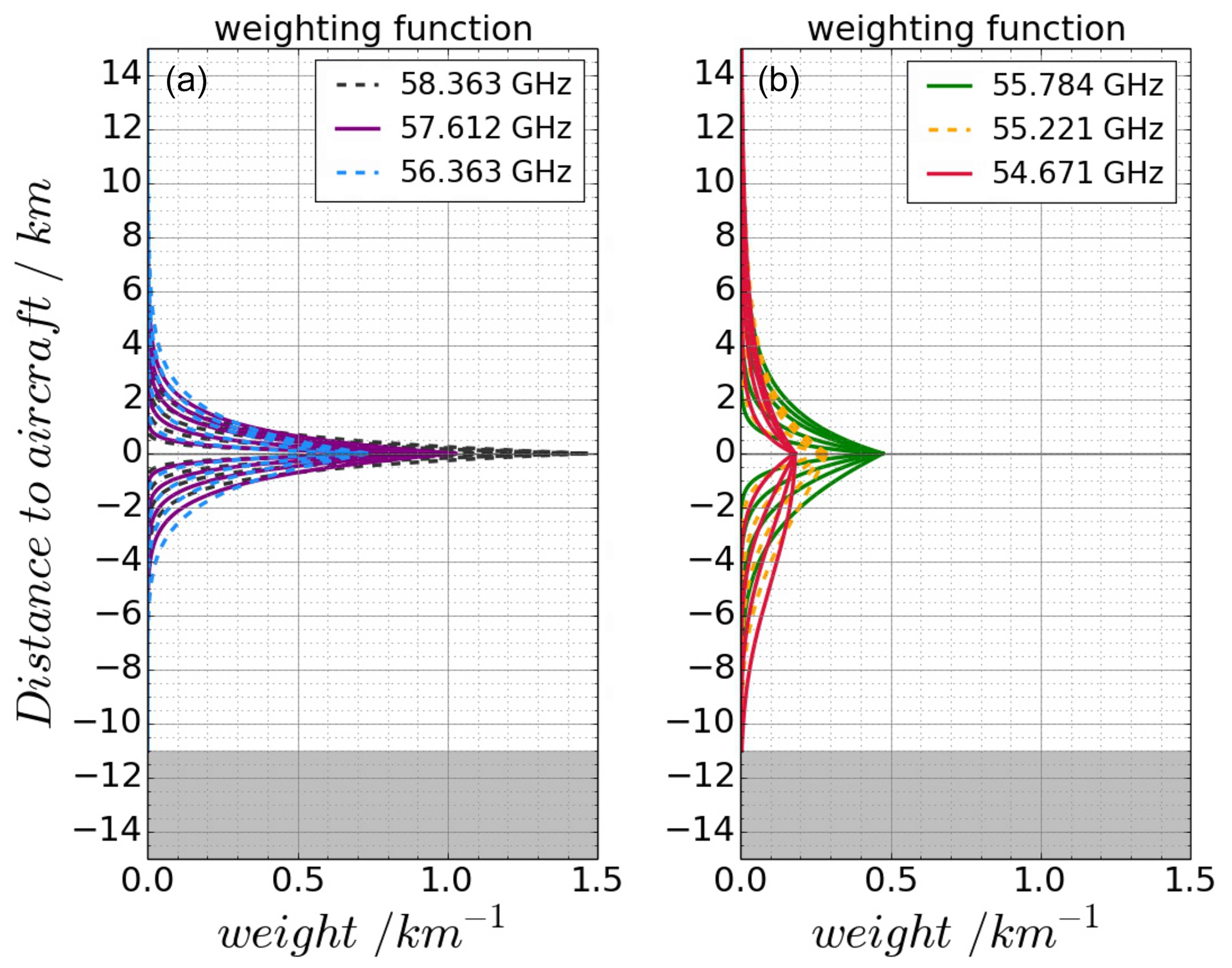
Figure A1 WFs (averaged over all contributing frequencies within filter transmission range) of the MTP frequency channels (each individual line corresponding to a different viewing angle), calculated at an aircraft altitude of 11 km. Shown are the three standard frequency channels (a) and three possible frequency channels (b) to be considered in a new measurement strategy for the HALO MTP. Grey areas at the bottom: altitude range that would be below the surface. Note that the black curves for the 58.363 GHz measurements are almost entirely covered by the other lines.

A1 Choice of LO frequencies

Logically, the best idea to widen the range of sensitivity would be to use different frequency channels that are located at weaker absorption lines than the standard frequency channels on the wing of the 60 GHz oxygen absorption complex or even between two lines, as was done with the older MTP instruments. However, the choice of an LO at the center frequency of an absorption line has several advantages: (i) the symmetrical line shape makes the retrieval more exact, (ii) synthesizer errors (small derivations of the LO from the intended frequency) cannot lead to large errors (opposite to a placement in which a strong line is placed just outside the filter range), and (iii) pressure broadening has an effect that is not as strong as with a placement between two lines. Concerning the threshold of possible frequencies, water vapor absorption becomes important in RT whenever frequencies close to 50 GHz are used.

To test the influence of opacity of the atmosphere, radiative transfer calculations were made in which the temperatures of all atmospheric layers between the ground and 110 km of altitude were set to 250 K. The simulation is made using the Temperature InveRsion Algorithm for MIcrowave SoUnding (TIRAMISU; Xu et al., 2016), a retrieval algorithm developed to process MTP brightness temperatures, which uses the radiative transfer model GARLIC. Simulations are made for the whole spectrum of frequencies between 50 and 60 GHz with 0.01 GHz resolution. This range includes the three standard frequency channels already in use, but also eight weaker absorption lines (Liebe et al., 1992). Furthermore, the simulations were carried out assuming six different flight altitudes between 2 and 15 km, which is the ceiling altitude of the HALO aircraft. In this setup, the expected brightness temperature for the horizontal and up-looking viewing directions is 250 K, unless the optical thickness of the atmosphere is small enough that the cold cosmic background influences the measurement, leading to a lower brightness temperature. The more transparent the atmosphere is at any frequency, the colder the simulated brightness temperature is, and the atmosphere close to the aircraft only contributes to a smaller part of the measured signal.

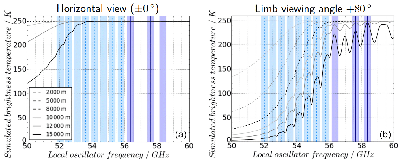
Figure A2 Simulated TBs at frequency channels between 50 and 60 GHz at different flight altitudes (different line styles) for a horizontal viewing angle (a) and a near-zenith angle (b). Solid vertical lines: standard frequency channels of the MTP; dashed vertical lines: strong lines that could be used as new MTP LOs. Shading around vertical lines: MTP filter width. Lines corresponding to altitudes of 8 km or lower overlap in panel (a).

The resulting brightness temperatures are shown in Fig. A2. Panel (a) shows those at a limb-viewing angle of 0^∘ (horizontal viewing direction) and panel (b) those at +80^∘ (near zenith). The solid black line in Fig. A2a shows that for any frequency channel below 54 GHz the atmosphere becomes partly transparent, even at the horizontal viewing angle. Hence, those measurements cannot be calibrated (or offset-corrected) using HALO TS, indicating that only frequency channels above 54 GHz should be considered. The results for the near-zenith measurements (Fig. A2b) indicate that the atmosphere is partly transparent for all possible frequency channels at nearly all flight altitudes. Whenever this transparency is too strong, the signal measured at weak absorption lines while looking downwards could be dominated by the surface temperature, which might not be well-known. As a result, for adding LOs to the MTP measurement strategy, only three possible frequency channels are considered: those corresponding to the oxygen absorption lines at 54.671, 55.221, and 55.784 GHz. The weighting functions of those three possible LOs under the standard set of elevation angles are shown in Fig. A1a. Obviously, the new frequency channels at weaker oxygen absorption lines are sensitive to a much wider range of altitude layers, especially below the aircraft. However, above the aircraft the weighting functions look similar to those of the standard frequency channels. This is due to the partial transparency of the atmosphere at these frequencies, indicated by low TBs in Fig. A2, combined with the fact that the viewing direction points through a medium that becomes optically thinner with increasing distance to the sensor.

A2 Choice of elevation angles

When discussing the choice of the set of elevation angles to be used in the MTP measurements, the signal path through the atmosphere has to be considered. Due to hardware design limitations, the range of MTP viewing angles is limited to ±80^∘. To consider a new, feasible set of elevation angles, it makes sense to compare the path lengths of all possible elevation angles α with the shortest possible path length through a vertical layer of the atmosphere at maximum elevation (±80^∘ relative to the horizon):

$$\begin{array}{}\text{(A3)}& l_{\text{rel}\mathrm{80}{}^{\circ }}={\displaystyle \frac{\cos \left(\mathrm{10}{}^{\circ }\right)}{\cos (\mathrm{90}{}^{\circ }-\mathit{\alpha })}}.\end{array}$$

The relative path lengths to the ±80^∘ angle are summarized in Table A1. The three largest elevation angles used in the standard MTP measurement strategy (underlined values in Table A1), in particular, do not differ much in their path lengths. This can result in the WFs of different measurements being very similar (overlaying lines, e.g., below aircraft altitude in Fig. A3); those measurements are (partly) redundant.

Table A1 Signal path lengths relative to ±80^∘. Values in italic font: elevation angles used in the standard measurement strategy. Values in bold font: possible candidates for a new strategy. Elevations in between, which are marked by (...), do not correlate with integer values in relative path lengths.

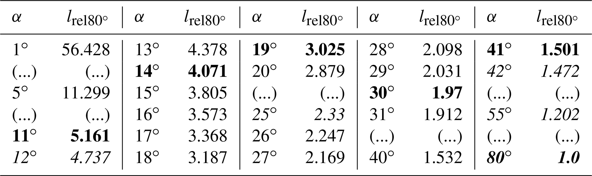
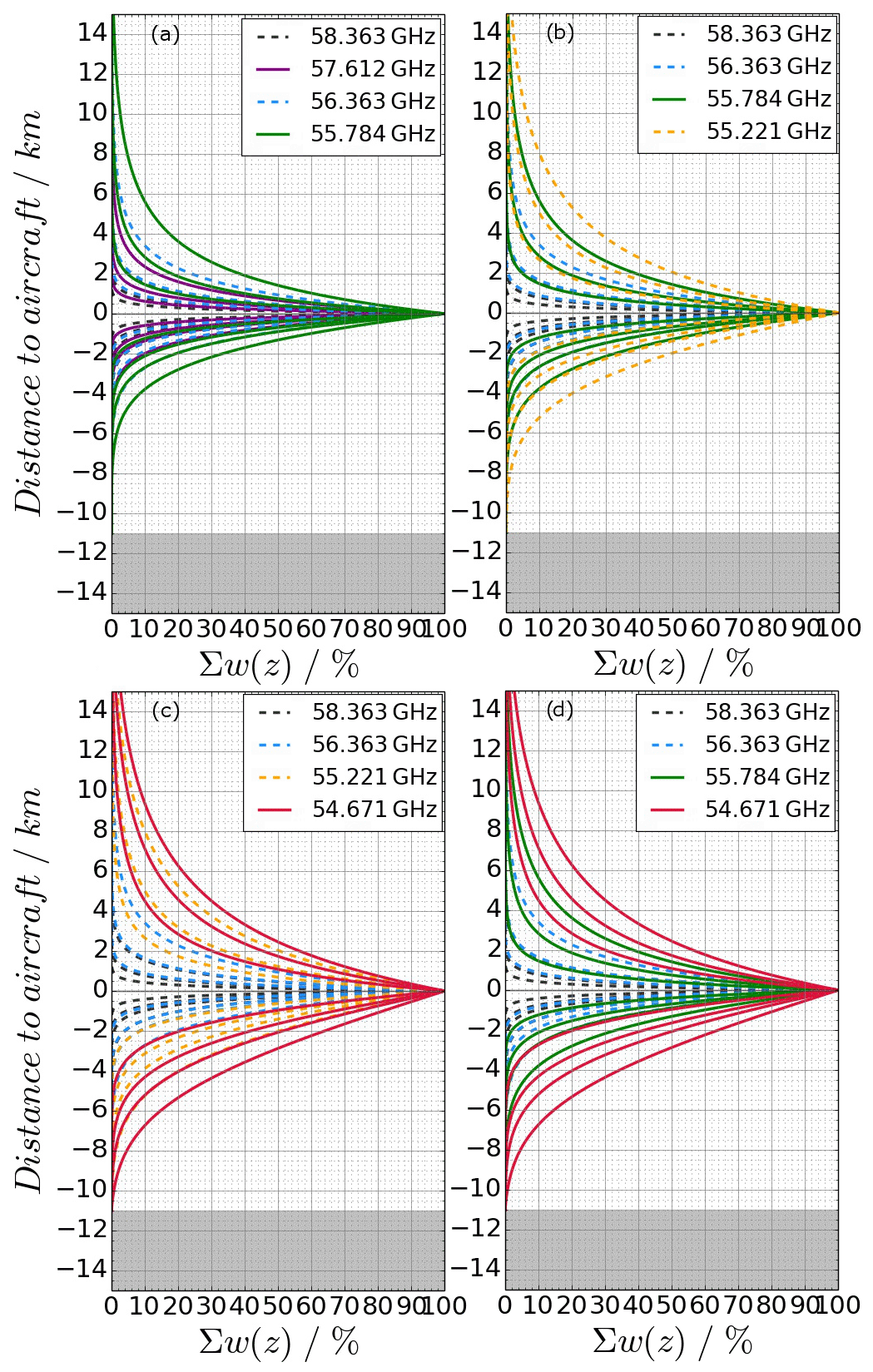
Figure A3 Cumulated weights of the MTP frequency channels (with each individual line in a panel corresponding to a different viewing angle and frequency combination) calculated for an aircraft altitude of 11 km. Shown are possible new measurement strategies, as mentioned in Table A2: (a) 8E4LOa, (b) 8E4LOc, (c) 8E4LOb1, and (d) 8E4LOb2. Grey areas at the bottom: altitude range that would be below the surface.

To derive a new set of elevation angles for MTP measurements with as much independent information as possible, a rule of thumb is used that with each new angle the length of the signal path at 80^∘ should be added, meaning that $l_{\text{rel}\mathrm{80}{}^{\circ }}$ is close to an integer. Corresponding rows are highlighted in grey in Table A1, including one angle with $l_{\text{rel}\mathrm{80}{}^{\circ }}\approx \mathrm{1.5}$. However, due to the fact that the antenna beam of the MTP instrument has a field of view of 7–7.5^∘, the measurements at 11 and 14^∘ would overlap and probably also not contain much different information from the measurement at 19^∘.

A3 Determining a new measurement strategy

Since the MTP is mounted on a moving platform with an approximate speed of 200 m s⁻¹, it is also necessary to consider the time it takes to record one complete measurement cycle. In favor of better horizontal resolution, the most appropriate set of elevation angles is ±14, ±30, ±41, and ±80^∘, considering the field of view of the antenna. Thus, including the horizontal measurement, only nine elevation angles would be used instead of the 10 standard angles, in which the down-looking set of angles is smaller than the up-looking set, leaving out the −55^∘ limb angle. Since the up-looking WFs of all possible frequency channels are very similar, the opposite would be more feasible: using more down-looking angles to enhance the resolution of measurements below the aircraft but reduce the number of up-looking angles, e.g., by leaving out the +41^∘ measurement.

Table A2 Proposed measurement strategies for future missions of the HALO MTP.

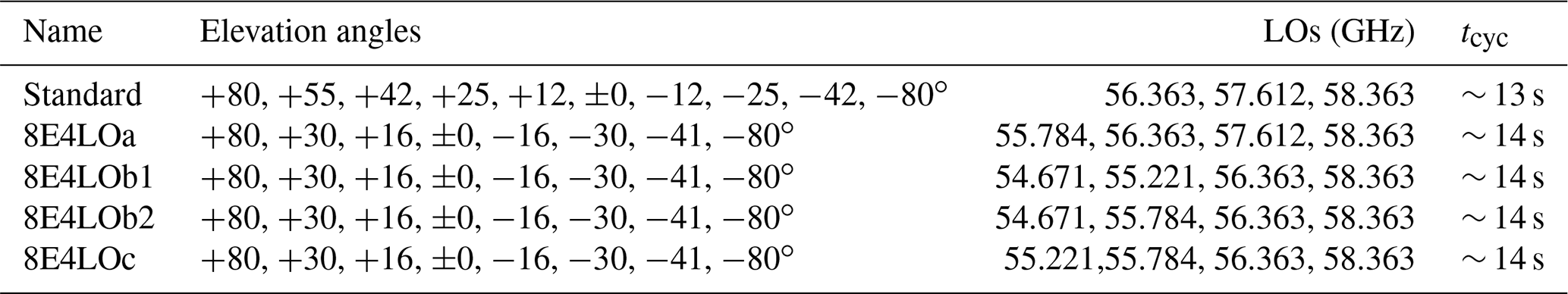
Based on all previous considerations, four new measurement strategies are proposed and summarized in Table A2. The new strategies are compromises between vertical resolution and range of sensitivity, keeping the total number of measurements per cycle close to the original so the total time of recording a complete measurement cycle does not change significantly, thus keeping the horizontal resolution of measurements. All proposed strategies use eight viewing angles and four frequency channels to enhance the vertical resolution and altitude range at the same time. The weighting functions of the measured signals for each of those new strategies are shown in Fig. A3. Depicted are the cumulative weights to indicate the percentage of the measurement signal that is acquired with decreasing distance to the aircraft. This depiction helps us to understand how much a certain layer of the atmosphere contributes to the total signal at a single viewing angle and frequency. If two lines in the figure overlap, the corresponding measurements (i.e., measurements at two certain frequency and viewing angle combinations) are redundant. To compare the relative contributions of different frequencies to the total incoming signal, please refer to Fig. A1.

Strategy 8E4LOa shows the result of simply adding a frequency channel to the standard set (Fig. A2a). In the other three proposed strategies, only two frequency channels of the original set are kept, and two frequency channels at weaker absorption lines are added. Since it is desirable to have the least redundancy in the measurement, overlaying weighting functions as seen, for example, in Fig. A2d are to be avoided. Also, if the aircraft is flying at lower altitudes, the frequency channel corresponding to the weakest absorption line might be influenced by the surface temperature. Hence, depending on the planned flight pattern, strategies 8E4LOb1 (Fig. A2c) or 8E4LOc (Fig. A2b) should be favored. The simple approach taken here indicates that both strategies increase the MTP measurement sensitivity to a wider altitude range, especially below flight level, while allowing for a well-resolved temperature retrieval and keeping the horizontal resolution of MTP data.

Obviously, the effects of changing the measurement strategy depend on the atmospheric conditions, mainly the true temperature profile around flight altitude. Hence, further investigations using forward radiative transfer calculations considering all MTP instrument characteristics shown in the main text would be needed to determine the influence of the proposed changes on retrieval input error and vertical measurement resolution. As the outcome clearly depends on the chosen retrieval algorithm, this is to be done in a separate study related to the retrieval algorithm used.