the Creative Commons Attribution 4.0 License.
the Creative Commons Attribution 4.0 License.
 | 12 Jan 2021
Separation of convective and stratiform precipitation using polarimetric radar data with a support vector machine method
Lin Tang
Pao-Liang Chang
Yu-Shuang Tang
A precipitation separation approach using a support vector machine method was developed and tested on a C-band polarimetric weather radar located in Taiwan (RCMK). Different from those methods requiring whole-volume scan data, the proposed approach utilizes polarimetric radar data from the lowest unblocked tilt to classify precipitation echoes into either stratiform or convective types. In this algorithm, inputs of radar reflectivity, differential reflectivity, and the separation index are integrated through a support vector machine. The weight vector and bias in the support vector machine were optimized using well-classified data from two precipitation events. The proposed approach was tested with three precipitation events, including a widespread mixed stratiform and convective event, a tropical typhoon precipitation event, and a stratiform-precipitation event. Results from the multi-radar–multi-sensor (MRMS) precipitation classification algorithm were used as the ground truth in the performance evaluation. The performance of the proposed approach was also compared with the approach using the separation index only. It was found that the proposed method can accurately classify the convective and stratiform precipitation and produce better results than the approach using the separation index only.
- Article
(15250 KB) - Full-text XML
- BibTeX
- EndNote


Convective and stratiform precipitation exhibit a significant difference in precipitation growth mechanisms, thermodynamic structures, and precipitation intensities (e.g., Houghton, 1968; Houze, 1993, 1997). For example, convective precipitation is generally associated with strong but small areal vertical air motion (>5 m s−1), but stratiform precipitation is associated with weak updrafts/downdrafts (<3 m s−1) (Penide et al., 2013). Convective precipitation also produces a higher rainfall rate (R) than the stratiform type (Anagnostou, 2004). Given the fact that the radar reflectivity (Z) from stratiform precipitation generally is less than 40 dBZ (Steiner et al., 1995) (hereafter SHY95), the R estimated from stratiform precipitation is less than 11 mm h−1 following the standard Marshall–Palmer relationship (Z=200R1.6). In order to obtain accurate rainfall estimation, different R(Z) relationships according to the precipitation types should be applied in quantitative precipitation estimation (QPE) (Kirsch et al., 2019). Therefore, accurately classifying precipitation into the either convective or the stratiform type can promote our understandings of cloud physics and thermodynamics and enhance QPE accuracy. For these purposes, numerous methods using ground in situ measurements or satellite observations were developed and applied during the past 40 years (e.g., Leary and House, 1979; Adler and Negri, 1988; Tokay and Short, 1996; Hong et al., 1999).
Ground-based weather radars, such as the Weather Surveillance Radar, 1988, Doppler (WSR-88D), are currently used in all aspects of weather diagnosis and analysis. Precipitation classification algorithms using single- or dual-polarization radars were developed during the past 3 decades. For a single-polarization radar, developed algorithms mainly rely on Z and its derived variables (e.g., Biggerstaff and Listemaa, 2000; Anagnostou, 2004; Yang et al., 2013; Powell et al., 2016). For example, SHY95 proposed a separation approach that utilizes the texture features derived from the radar reflectivity field. In this approach, a grid point is identified as the convective center if its Z value is larger than 40 dBZ or exceeds the average intensity taken over the surrounding background. Those grid points surrounding the convective centers are classified as convective area, and far regions are classified as stratiform. Penide et al. (2013) found that SHY95 may misclassify those isolated points embedded within stratiform precipitation or associated with low cloud-top height. Powell et al. (2016) modified SHY95's approach, and the new approach can identify shallow convection embedded within large stratiform regions. A neural-network-based convective–stratiform classification algorithm was developed by Anagnostou (2004). Six variables were used in this approach as inputs, including storm height, reflectivity at 2 km elevation, the vertical gradient of reflectivity, the difference in height, the standard deviation of reflectivity, and the product of reflectivity and height. Similar variables were also used in a fuzzy-logic-based classification approach proposed by Yang et al. (2013).
Motivations of developing a new classification algorithm are mainly based on two aspects. First, according to the U.S. Radar Operations Center (ROC), the WSR-88D radars are currently operated without updating a complete volume during each volume scan, especially during precipitation events. New radar scanning schemes are designed to update data from low elevations at a high frequency and data from high elevations at a low frequency. Such an alternative scanning scheme enables the WSR-88D radars to promptly capture the storm development and enhance the weather forecast capability. These new schemes include the automated volume scan evaluation and termination (AVSET), supplemental adaptive intra-volume low-level scan (SAILS), the multiple elevation scan option for SAILS, and the mid-volume rescan of low-level elevations (MRLEs). With these new scanning schemes, the separation of stratiform/convective becomes a challenge for those algorithms requiring a full-volume scan of data. Therefore, a separation algorithm using only low tilt radar data is desired. The second reason is to further explore the applications of the polarimetric variables. Polarimetric weather radars have been well applied in radar QPE, severe weather detection, hydrometeor classification, and cloud microphysics retrieval (Ryzhkov and Zrnic, 2019; Zhang, 2016). Extra information about hydrometeors' size, shape, and orientation could be obtained through transmitting and receiving electromagnetic waves along the horizontal and vertical directions. Polarimetric measurements may reveal more precipitation microphysical and dynamic properties. Inspired by these features, a C-band polarimetric radar precipitation separation approach was developed by Bringi et al. (2009) (hereafter BAL), which classifies the precipitation into stratiform, convective, and transition regions based on retrieved drop size distribution (DSD) characteristics. However, it was found that strong stratiform echoes might have similar DSDs to weak convective echoes and lead to wrong classification results (Powell et al., 2016).
In this work, a support-vector-machine-(SVM)-based classification method was developed and tested on a C-band polarimetric radar located in Taiwan. Unlike some existing classification techniques that require a whole-volume scan of data, this new approach only requires the lowest unblocked tilt data in the separation. If the lowest tilt is partially or completely blocked, the next adjacent unblocked tilt is used in the classification instead. This method's major advantage is that it can provide classification results even when the radar is operated under AVSET, SAILS, and MRLE scanning schemes. This paper is organized as follows: Sect. 2 introduces the proposed method, including radar variables and data processing, the SVM method, and the training process. The performance evaluation is shown in Sect. 3, and the discussion and summary are given in Sect. 4.
In the current work, the SVM precipitation separation approach was developed and validated on a C-band polarimetric radar (RCMK) located at Makung, Taiwan (Fig. 1). The Weather Wing of the Chinese Air Force deployed this radar and has made the data available to the Central Weather Bureau (CWB) of Taiwan since 2009. Together with three single-polarization S-band WSR-88D (RCCG, RCKT, and RCHL) and one dual-polarization S-band radar (RCWF), these five radars provide real-time products to CWB to support missions of flood monitoring and prediction, landslide forecasts, and water resource management. The wavelength of RCMK is 5.291 cm, and its range and angular resolutions are 500 m and 1∘, respectively. RCMK performs volume scans of 10 tilts (0.5, 1.4, 2.4, 3.4, 4.3, 6.0, 9.9, 14.6, 19.5, and 25∘) every 5 min. The Central Mountain Range (CMR) of Taiwan is also shown in Fig. 1, which poses a major challenge to radar products. Radars located in complex terrain are prone to partial or total blockages, which cause data from low elevation angles (EAs) to be unavailable or problematic. Blockage maps of RCMK are illustrated in Fig. 2. Since there are severe blockages at 0.5∘ for RCMK, data from the 1.4∘ EA are used in the algorithm development.
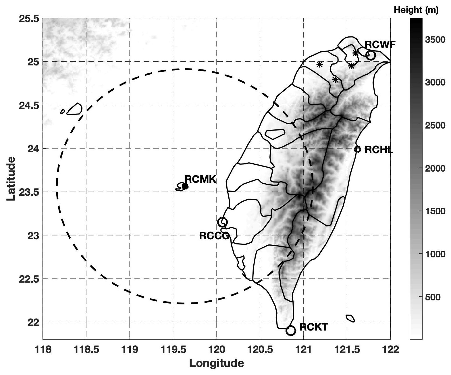
Figure 1The terrain of Taiwan, the location of a C-band polarimetric radar RCMK (marked with a black square), JWDs (marked with black stars), and four S-band single-polarization radars: RCCG, RCKT, RCHL, and RCWF (marked with black circles). The continuous grayscale terrain map shows the central mountain range of Taiwan.

Figure 2Blockage maps of RCMK from the first two EAs (0.5 and 1.4∘). The grayscale indicates the blockage percentages.
2.1 Input polarimetric radar variables and preprocesses
Three measured or derived radar variables are proposed as inputs to the SVM approach: Z, differential reflectivity fields (ZDR), and separation index (i). Because convective precipitation generally shows higher reflectivity values, Z works well as one of the inputs in most of the precipitation classification approaches. For example, a radar echo, with the reflectivity of 40 dBZ and above, is automatically classified as a convective type in the approach developed by SHY95. Differential reflectivity, which is highly related to a raindrop's mass-weighted mean diameter (Dm), is another good indicator of precipitation type. It was found that the values of Dm in stratiform and convective precipitation generally are within 1–1.9 mm and above 1.9 mm, respectively (Chang et al., 2009). Therefore, higher ZDR values are expected from convective than from stratiform precipitation.
For short-wavelength radars such as C-band or X-band radars, the Z and ZDR fields will be significantly attenuated when the radar beam propagates through heavy-precipitation regions. Both the Z and ZDR fields need to be corrected from attenuation before applied in the precipitation classification and QPE. Different attenuation correction methods were proposed using the differential phase (ϕDP) measurement such as the linear ϕDP approach, the standard ZPHI method, and the iterative ZPHI method (e.g., Jameson, 1992; Carey et al., 2000; Testud et al., 2000; Park et al., 2005). Because of its simplicity and easy implementation in a real-time system, the linear ϕDP method was applied in the current work.
where Z′(r) (ZDR′(r)) is the observed reflectivity (differential reflectivity) at range r; Z(r) (ZDR(r)) is the corrected value; ϕDP(0) is the system value; ϕDP(r) is the smoothed (by FIR filter) differential phase at range r. The attenuation correction coefficients α and β depend on DSD, drop size shape relations (DSR), and temperature. The typical range of α (β) is found to be 0.06∼0.15 (0.01∼0.03) dB per degree for C-band radars (e.g., Carey et al., 2000; Vulpiani et al., 2012). Following the work from Wang et al. (2014), optimal coefficients α and β in Taiwan are 0.088 and 0.02 dB per degree, respectively. The Z and ZDR fields are further smoothed with a 3×3 (along azimuthal angle and along range) moving window function after being corrected from attenuation.
Other quality control issues on Z and ZDR fields, including calibration, vertical profiles of reflectivity (VPR) correction, and ground clutter removal, were also considered in this work. First, since this radar is used for the real-time QPE purpose, the calibration biases of Z and ZDR should be within 1 and 0.1 dB, respectively. The data quality of RCMK was examined through validating the QPE performance in different works (e.g., Wang et al., 2013, 2014). Therefore, the calibration biases (Z and ZDR) of RCMK should be within reasonable ranges. Second, a VPR correction is generally needed on the reflectivity field to reduce the measurement biases because of the melting layer (Zhang et al., 2011). The enhanced backscattering amplitudes of melting hydrometeors within the melting layer (bright band) significantly enhance radar reflectivity. The bright band feature is one of the obvious indicators of stratiform precipitation and can normally be observed from relatively high EAs (such as above 9.9∘). Given the fact that data from the 1.4∘ elevation angle are used within the maximum range of 150 km and the melting layer is usually around 5 km in Taiwan, the radar data used in this work are well below the melting layer. Therefore, no VPR corrections are applied to the fields of Z and ZDR. Third, since ground clutter is typically associated with a low correlation coefficient (ρHV), a ρHV threshold of 0.85 is used in the current work to remove radar echoes from ground clutter (Park et al., 2009).
Another input variable is the separation index i, which was initially proposed by BAL. The i was calculated under a normalized gamma DSD assumption:
where is the estimated NW (normalized number concentration) from observed Z and ZDR and is calculated as
In Eq. (4), D0 is the median volume diameter and can be calculated as
The units of ZDR, Z, Nw, and D0 are dB, mm6 m−3, mm−1 m−3, and mm, respectively. The positive and negative values of index i indicate convective and stratiform rain, respectively, and indicates transition regions (Penide et al., 2013). BAL pointed out that index i worked well in most of the cases in their study; however, incorrect classification results are likely obtained for low-Z and high-ZDR cases in some convective precipitation.
2.2 Drop size distribution and drop shape relation
It should be noted that the relations between i, Nw, and D0 were derived using the DSD data collected in Darwin, Australia. Coefficients in Eqs. (2)–(5) need to be adjusted according to the radar frequency and/or DSD and DSR features from the specific location (Thompson et al., 2015). In the current work, the separation index i is directly derived using Eqs. (2)–(5) without further adjustment. It was shown by Wang et al. (2013) that DSD and DSR features in Taiwan are very similar to those measured in Darwin, Australia. Similar R(KDP) relationships were obtained using data collected from these two locations. Coefficients derived by BAL could be directly used in Taiwan without further modification. To verify this assumption, Nw and D0 were calculated using DSD data collected from four impact-type Joss–Waldvogel disdrometers (JWDs) located in Taiwan (Fig. 1). The measurement range and temporal resolution of these JWDs are 0.359–5.373 mm and 1 min, respectively. A total of 4306 min of data from 2011–2014 is used in Nw and D0 calculation following the approach described in Bringi et al. (2003). Similar to the work presented in BAL, the distribution of i along median volume diameter D0 is shown in Fig. 3. Sample pairs (log 10Nw, D0) from stratiform and convective types are represented with gray circles and black stars, respectively. Although the relation described in Eq. (3) can separate most stratiform from convective types, a large number of points are still classified incorrectly. Therefore, the single separation index is not sufficient in the precipitation separation, and other variables such as Z and ZDR may be used as supplements.
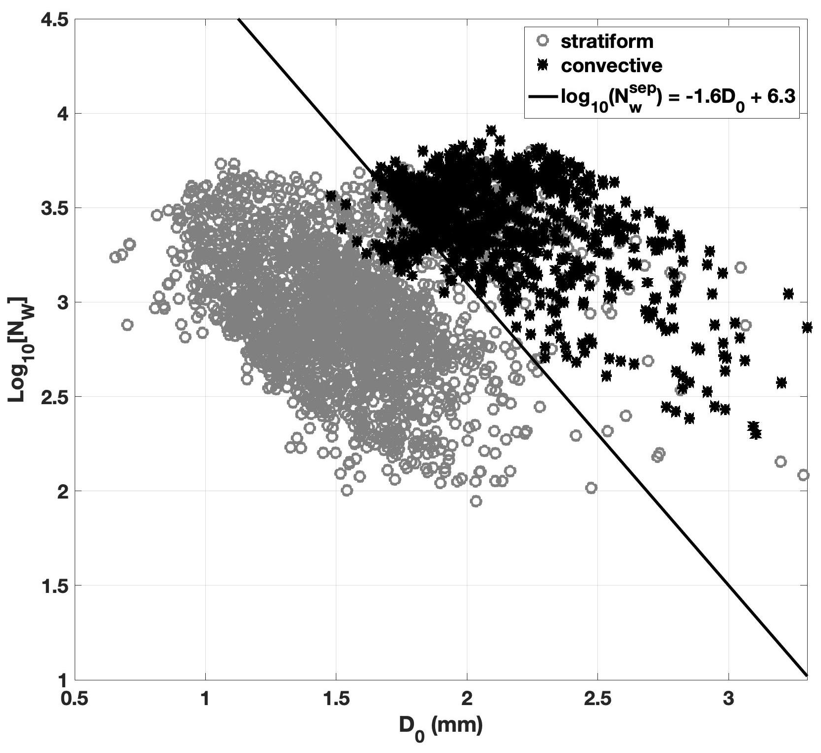
Figure 3The distribution of log 10(Nw) vs. D0. The DSD data from stratiform and convective precipitation are presented with gray circles and black stars, and the separator line is shown with a solid line.
2.3 Support vector machine (SVM) method
2.3.1 Introduction of SVM
Artificial intelligence (AI) algorithms using meteorological radar data have been developed well during the past 2 decades. With the assistance of AI, weather radar's capabilities in severe weather prediction, rainfall rate estimation, and lightning detection have apparently been improved (e.g., Capozzi et al., 2018; T. et al., 2019; Yen et al., 2019). Inspired by these enhancements, a precipitation separation approach using an SVM was developed and tested in the current work. Generally, an SVM can be viewed as a kernel-based machine learning approach, which nonlinearly maps the data from the low-dimension input space to a high-dimension feature space and then linearly maps to a binary output space (Burges, 1998). Given a set of training samples, the SVM constructs an optimal hyperplane, which maximizes the margin of separation between positive and negative examples (Haykin, 2011). Specifically, given a set of training data , the goal is to find the optimal weights vector W and a bias b such that
where Xi∈ℝm is the input vector, m is the variable dimension (m = 3 in this work), N is the number of training samples, and yi is the output with the value of +1 or −1 that represents convective or stratiform types, respectively. The particular data points (Xi,yi) are called support vector if Eq. (6) is satisfied with the equality sign. The optimum-weight vector W and bias b can be obtained through solving the Lagrangian function with the minimum cost function (Haykin, 2011).
Since the SVM can be viewed as a kernel machine, finding the optimal weight vector and bias in Eq. (6) can be alternatively solved through the recursive least square estimations of
where Ns is the number of support vectors, αi is the Lagrange multipliers, and k(X,Xi) is the Mercer kernel defined as
With the solved , the SVM calculates the classification results with new input data Z∈ℝm as
When f(Z)=1, the output is classified as convective; otherwise it is stratiform.
2.3.2 Training of the SVM
In the SVM approach, the weight vector and bias in Eq. (6) and the standard deviation vector in Eq. (8) need to be optimized through a recursive least square estimation using training data. Since the training data play a critical role in the SVM approach, Z, ZDR, and i from convective- and stratiform-precipitation events were carefully examined in three steps. Firstly, the training data were checked following general classification principles. For example, training data from convective precipitation are generally associated with relatively large reflectivity and high vertically integrated liquid (VIL). On the other hand, stratiform precipitation is generally associated with prominent bright band signatures. Secondly, the precipitation type is verified by ground observation, such as ground severe storm reports. Thirdly, the precipitation type is confirmed by the multi-radar–multi-sensor (MRMS) precipitation classification algorithm implemented in Taiwan (Zhang et al., 2011, 2016). In this MRMS classification approach, a three-dimensional radar reflectivity field is mosaicked from four S-band single-polarization radars (Fig. 1). The composite reflectivity (CREF) and other measurements, such as temperature and moisture fields, are then used in the surface precipitation classification (Zhang et al., 2016). The performance of MRMS has been thoroughly evaluated for years in QPE, flash flood monitoring, severe weather observation, and aviation weather surveillance (e.g., Gourley et al., 2016; Smith et al., 2016). It was found that MRMS system can provide robust and accurate products, and these products were used as benchmarks and/or ground truths in many studies (e.g., Grecu et al., 2016; Skofronick-Jackson et al., 2017). Moreover, since the MRMS classification is a mosaicked product derived from four S-band radars, it can be viewed as an independent reference. Therefore, the MRMS precipitation classification is regarded as the appropriate reference in training and validation.
Convective-type training data are mainly from a precipitation event on 23 July 2014. Apparent squall line features could be identified from this thunderstorm, and MRMS classified this precipitation event as the convective type. Strong downdrafts triggered by this storm caused an aircraft crash at the airport of Makung at 11:06 UTC. Radar data collected from 10:30 to 11:30 UTC were used as the convective-type data, and data selection follows the criteria of Z>20 dBZ and ρHV>0.9. Some samples from a mixed stratiform- and convective-precipitation event on 30 August 2011 are also included as convective-type data. The stratiform-type data are from the precipitation event on 30 August 2011, and only those data identified as a stratiform type by MRMS are used in training. It should be noted that the ρHV threshold of 0.9 is used in the training data selection for both convective and stratiform precipitation. As reported in Park et al. (2009), the liquid phase precipitation (e.g., light to heavy rain) is associated with relatively high ρHV (>0.92). Other types of precipitation, such as the mixture of rain and hail, wet snow, and crystals, may produce low ρHV (<0.85). Since the i is derived based on the raindrop size distribution assumption, the proposed SVM approach is only valid for liquid phase precipitation classification. The classification of other types of precipitation is beyond the scope of this work. Therefore, 0.9 is a reasonable ρHV threshold in the training data selection. The training data used in this work are from pure liquid precipitation events, and the average ρHV is above 0.98. Similar training results are expected if a higher ρHV threshold is used in the training data selection.
A total of 17 281 data sets (15 144 sets of stratiform data and 2137 sets of convective data) are used in the training process. One data set is defined as the variables from a gate in terms of range and azimuthal angle. To be more specific, a set of training data means a vector of [], where a and r indicate azimuthal angle and range, respectively. The variable d is the ground truth (with representing convective or stratiform types), and acts as the desired response in the training process. It should be noted that the size of training data is regarded as small, and the ratio between convective and stratiform data is not well balanced. Much more data from various precipitation events should be included in the training process if the proposed algorithm is implemented in operation.
The number of support vectors is selected as 1000 in the current work, and the training process is regarded as completed when the root-mean-square error reaches a stable value. In the SVM approach, the original three-dimensional input space nonlinearly maps to a 1000-dimensional feature space and then linearly maps to a binary output space (Burges, 1998). The higher-dimension feature space (the number of support vector) potentially captures more input variables features with higher computation cost. Generally, after the number of support vector reaches a particular number, the enhancement of the SVM approach becomes slight. There is a balance between accuracy and computation cost. In the current work, the number of support vectors was tested with a value of 500, 750, 1000, 2000, and 5000. Since 1000 support vectors can produce less than 5 % error with reasonable computation time, they are used in the current work.
3.1 Description of the experiments
The performance of the proposed approach was validated with three precipitation events from 2009 to 2011: one stratiform precipitation, one intense tropical precipitation, and one mixed convective and stratiform precipitation. In the validation, a ρHV threshold of 0.85 is first used to remove radar echoes not associated with liquid phase precipitation such as clutter and AP (Park et al., 2009). As discussed in Sect. 2.3.2, some ice phased or mixed precipitation such as snow, the mixture of hail and rain, and crystals may be associated with low ρHV (<0.85). However, this work proposes an approach to classify liquid phase precipitation into either stratiform or convective types. Classification of other meteorological targets is beyond the scope of this work. Two experiments based on the BAL approach with different thresholds (i.e., BAL0 and BAL−0.5) were also validated with the same events. In these two experiments, the separation index i from each radar gate was first calculated using Eqs. (2)–(5), and thresholds of T0=0 and −0.5 were then used to separate convective type from stratiform type. A gate is classified as convective type if the obtained i is larger than T0 and as stratiform type otherwise. It was suggested that positive (negative) i is generally associated with convective (stratiform) precipitation (Bringi et al., 2009). Therefore, T0 = 0 was selected as one of the thresholds. Another aggressive threshold of −0.5 was also tested in the current work, which will classify many more pixels as convective. Performances of those approaches requiring multiple elevation angles as introduced in Sect. 1 are not discussed in this work.
In the evaluation, three statistical scores of probability of detection (POD), false alarm rate (FAR), and critical success index (CSI) are used, and MRMS classification results are used as the “ground truth” in the calculation.
where “hit,” “false,” and “miss” are, respectively, defined as a radar gate classified as convective type by MRMS and the evaluated approach simultaneously, by the evaluated approach only, and by MRMS only. Since these scores only partially capture the performance due to the time gap between MRMS and RCMK results (SVM and BAL), a new evaluation score RCS (whole coverage convective ratio) is also used as a supplement:
where Ncon and Nstr are the total pixel numbers of convective and stratiform types within the coverage, respectively. The evaluation results are shown in the following sections.

Figure 4The time series plot of RCS (a), CSI (b), POD (c), and FAR (d) from 30 August 2011. 24 h data (00:00–24 00 UTC) are used in each case. The results from BAL with the threshold , BAL with the threshold T0=0, SVM, and MRMS are presented by green, blue, red, and black lines, respectively.
3.2 Experiment results
3.2.1 Widespread mixed stratiform and convective precipitation
The performance of the proposed approach was first validated with one widespread stratiform and convective mixed precipitation event on 30 August 2011, and 24 h data (00:00–24:00 UTC) were used in the evaluation. Classification results from the proposed SVM were calculated with the trained weight vector and biases, and results from the BAL approach (BAL0 and BAL−0.5) were also calculated for the comparison purpose. It should be noted that the threshold of −0.5 is much lower than the value suggested by BAL, and BAL−0.5 will classify more precipitation as the convective type.
Figure 4 shows the time series of RCS (a), CSI (b), FOD (c), and FAR (d) are calculated using Eqs. (10)–(13), where results from MRMS, SVM, BAL0, and BAL−0.5 are represented by black, red, blue, and green lines, respectively. When the MRMS results are applied as the ground truth, BAL0 obviously classifies more precipitation as stratiform type during this 24 h period. The time series of RCS from BAL0 are much lower than the other three approaches. BAL−0.5 classifies more pixels as convective than BAL0, as expected, and the RCS scores are much higher than BAL0. The proposed SVM shows the most similar RCS scores to MRMS compared to BAL approaches. Since BAL−0.5 uses a very low threshold, it classifies more pixels as convective type, and the obtained RCS scores are higher than MRMS. SVM and BAL−0.5 show similar results in terms of CSI, POD, and FAR, but BAL0 shows apparently worse performance.
To better understand the performance of each approach, the classification results and radar variables (Z, ZDR, and i) from two distinct moments are examined as shown in Figs. 5–7. Figure 5 shows the classification results from 03:03 UTC, 30 August 2011, where BAL0, BAL−0.5, SVM, and MRMS are shown in panels (a), (b), (c), and (d), respectively. The time stamp for the MRMS result is 03:00 UTC and about 3 min earlier than the other three approaches. Three input variables of SVM at 03:03 UTC are shown in Fig. 6, where Z, ZDR, and i are presented in panels (a), (b), and (c). A circle is inserted in Figs. 5 and 6 to emphasize a region where BAL and SVM show different performances. Within this circle, BAL0 (BAL−0.5) classifies the least (most) echoes as convective and SVM shows the most similar results to MRMS. The averages of Z and ZDR within this region both show relatively large values (Z>36 dBZ and ZDR>0.75 dB) as shown in Fig. 6. This is a clear indication of convective-type precipitation. Both SVM and BAL−0.5 classify most of the area within the red circle as convective, and this result is consistent with the MRMS result. Since the separation indexes within the black circle are below or slightly higher than 0, most of the area is classified as stratiform type by BAL0. For this moment, the threshold of −0.5 shows better performance than 0. Similar reasons may be applied to other regions.
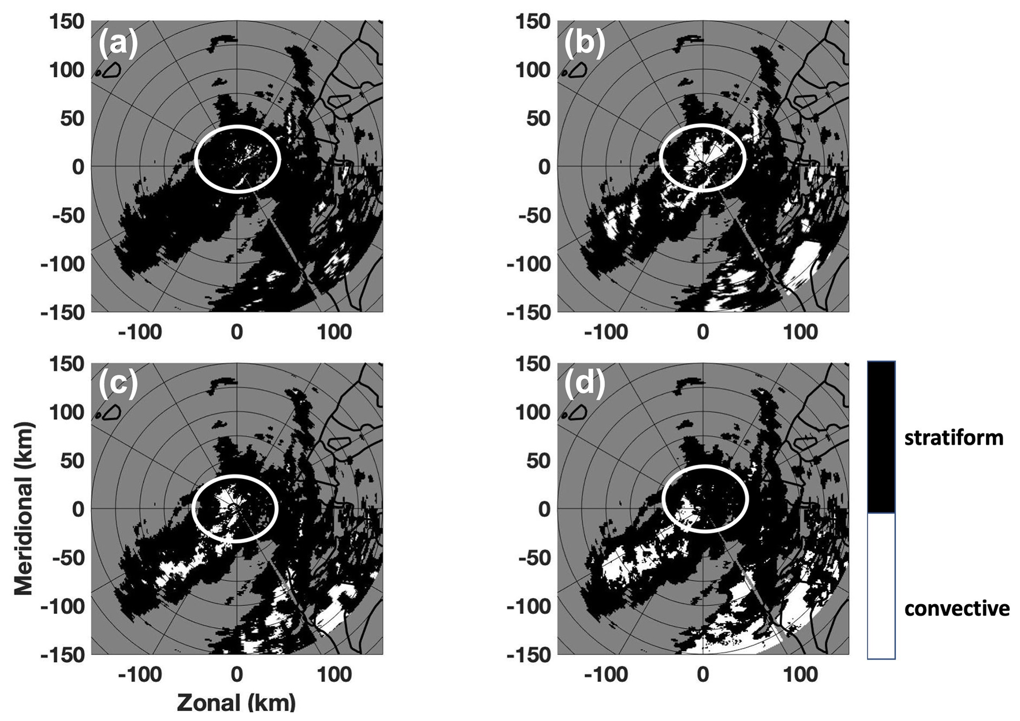
Figure 5The classification results from BAL0 (a), BAL−0.5 (b), SVM (c), and MRMS (d). The time stamp for BAL0, BAL−0.5, and SVM is 03:03 UTC, 30 August 2011, and time stamp for MRMS is 03:00 UTC, 30 August 2011. The region inside the white circle is used in the analysis.
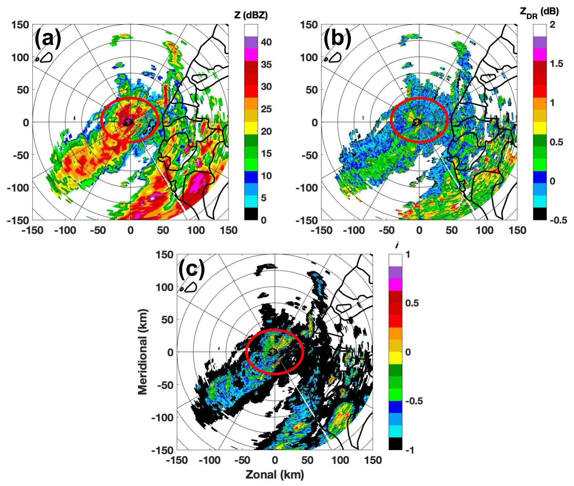
Figure 6Radar variables of reflectivity (a), differential reflectivity (b), and separation index (c). The radar data were collected by RCMK at 03:03 UTC, 30 August 2011. The region inside the red circle is used in the analysis.
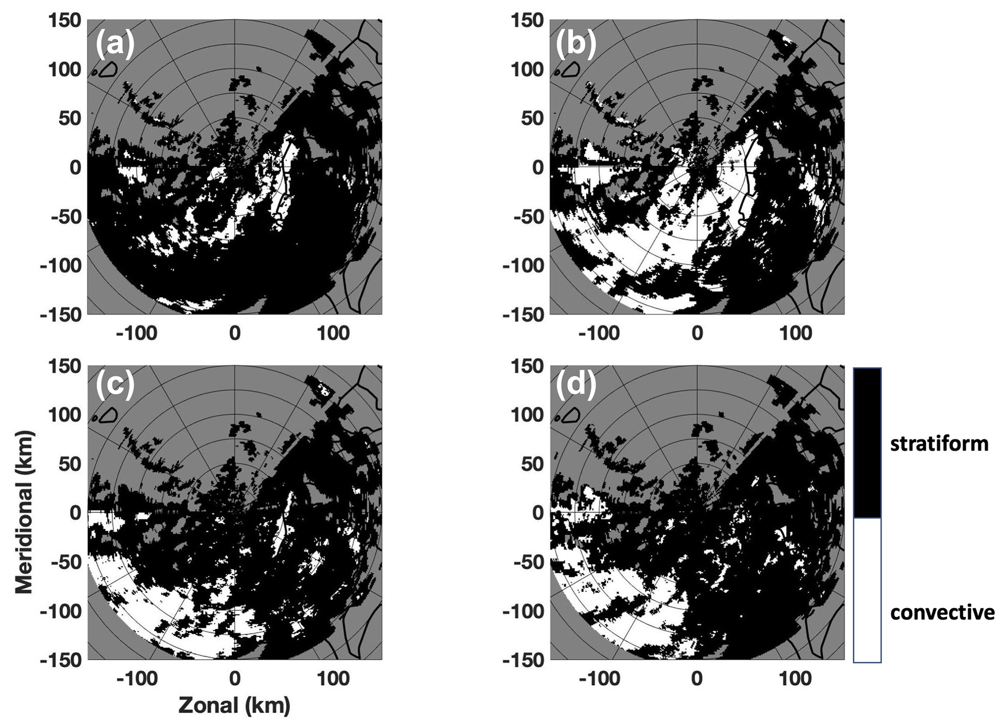
Figure 7Similar to Fig. 5, results are from 06:50 UTC.
Figure 7 shows another example of classification results from 06:50 UTC. At this moment, although SVM and BAL−0.5 produce similar CSI (0.30 vs. 0.25) and POD (0.48 vs. 0.52), the RCS from BAL−0.5 (32 %) is much higher than RCS from MRMS (17 %) and SVM (13 %). These scores could also be found in Fig. 4. In Fig. 7, It could be found that the MRMS, SVM, and BAL−0.5 show similar classification results between the azimuthal angle of 180 and 270∘. However, BAL−0.5 misclassifies gates between 90 and 180∘ as convective type, which produces such high RCS. On the other hand, MRMS and SVM show similar classification results in this region.
3.2.2 Tropical convective
Typhoon Morakot (6–10 August 2009) brought significant rainfall to Taiwan. Over 700 people were reported dead in the storm, and the property loss was more than USD 3.3 billion. For most of the time during its landfall in Taiwan, the precipitation was classified as a mixture of tropical convective and tropical stratiform types. The performances of SVM, BAL0, and BAL−0.5 were validated using 96 h data from 6 to 9 August 2009, where the results from 10 August 2009 were not included in the evaluation because no significant precipitation was observed from that day. Figure 8 shows the time series plots of RCS (a), CSI (b), POD (c) and FAR (d). It could be found that scores of RCS, CSI, and POD from the BAL-based approaches are evidently lower than the results from SVM and MRMS, and the latter two show similar performance during these 4 d.
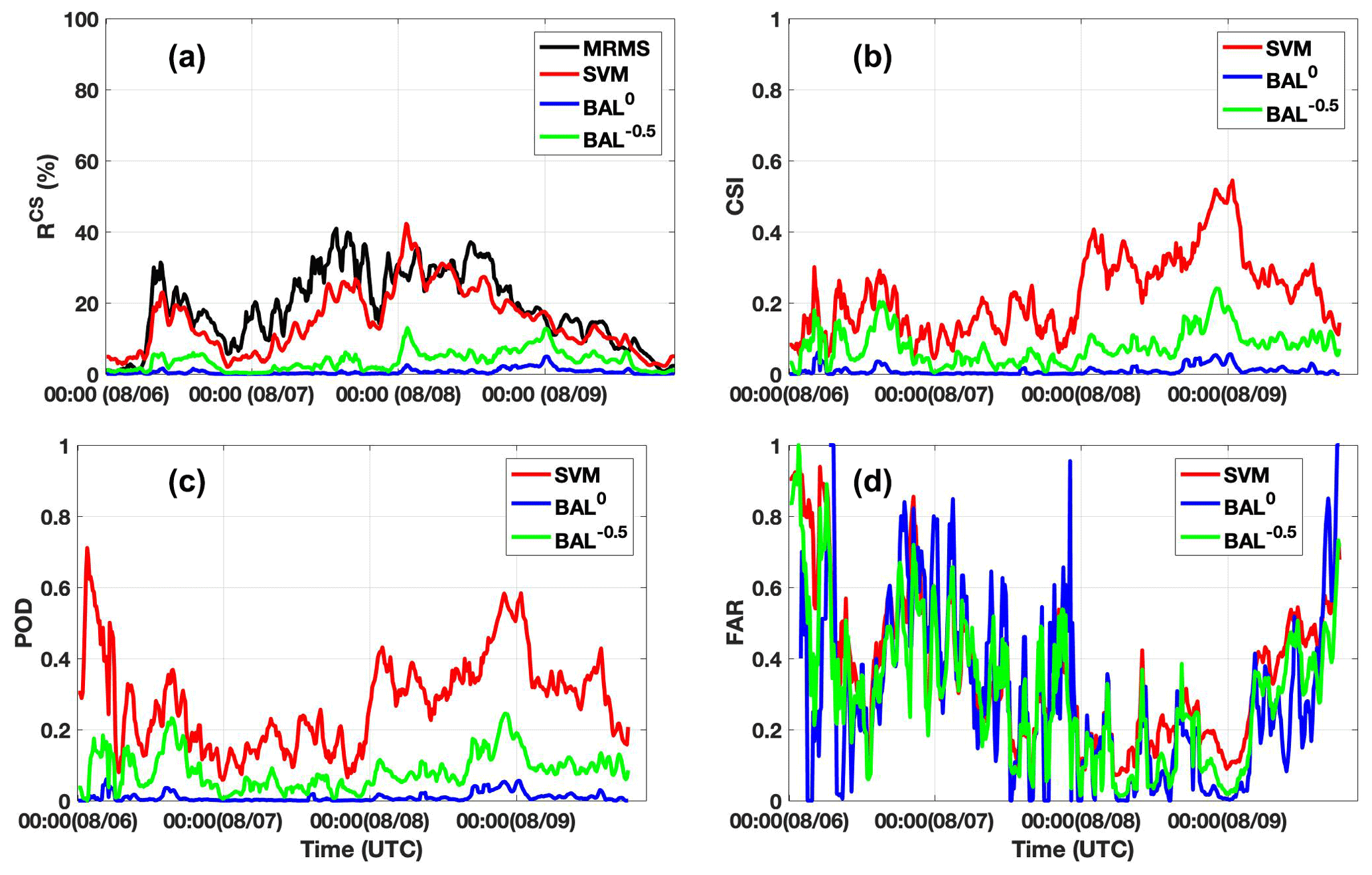
Figure 8The time series plot of RCS (a), CSI (b), POD (c), and FAR (d) from 6–9 August 2009; 96 h data are used in each case. The results from BAL with the threshold , BAL with the threshold T0=0, SVM, and MRMS are indicated by green, blue, red, and black lines, respectively.
Classification results from BAL0, BAL−0.5, SVM (0402 UTC), and MRMS (04:00 UTC) from 9 August 2009 are shown in Fig. 9a–d, respectively. The classification results within two regions, highlighted with two circles, are convective (SVM and MRMS) and stratiform (BAL0 and BAL−0.5). Radar variables from 04:02 UTC are shown in Fig. 10 including the reflectivity (a), differential reflectivity (b), and separation index (c). Figure 10d is the zoom-in reflectivity field inside the red rectangular box (a) for more details. It was found that a heavy precipitation band is over RCMK (Fig. 10d), and this may cause significant attenuation in Z and ZDR fields. Although both Z and ZDR fields were corrected using Eq. (1), deficient or excessive compensations in Z and ZDR fields lead to increased uncertainty in the separation index. It may be the primary reason for the small values of the separation index. Other reasons such as wet radome may also contribute to the Z and ZDR issues. In Fig. 10c, the separation index i is equal to or less than −0.5 in the circled areas, and the BAL-based approaches classify these regions as stratiform. On the other hand, these regions clearly show the convective-precipitation features in the fields of Z (Fig. 10a) and ZDR (Fig. 10b).
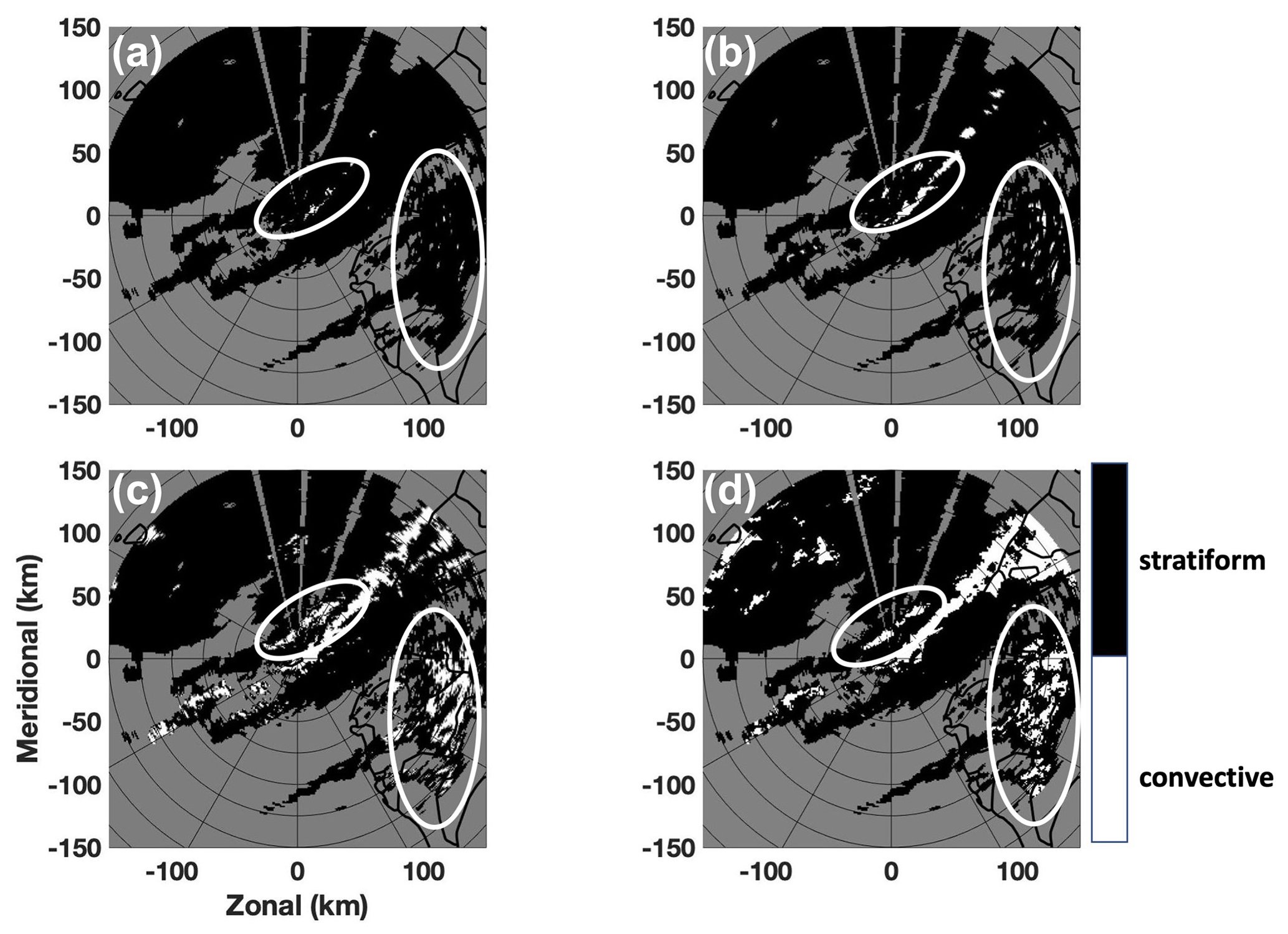
Figure 9The classification results from BAL0 (a), BAL−0.5 (b), SVM (c), and MRMS (d). The time stamp for BAL0, BAL−0.5, and SVM is 04:02 UTC, 9 August 2009, and the time stamp for MRMS is 04:00 UTC, 9 August 2009.
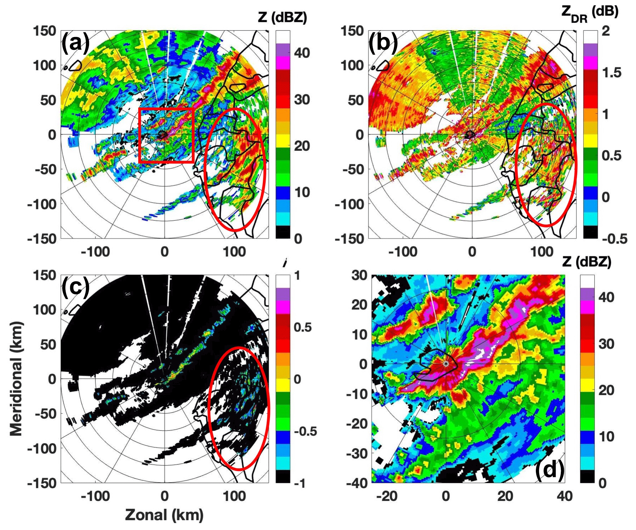
Figure 10Radar variables of reflectivity (a), differential reflectivity (b), separation index (c), and (d) reflectivity within the red rectangular in (a). The radar data were collected by RCMK at 04:02 UTC, 9 August 2009.
3.2.3 Stratiform-precipitation event
The performances of BAL0, BAL−0.5, and SVM were also evaluated with a widespread stratiform-precipitation event on 26 March 2011. This is a typical stratiform-precipitation event, and there were no convective-type pixels identified by MRMS. These three approaches showed consistent classification results with the MRMS result during an 8 h period evaluation. For all three approaches, the scores of POD, FAR, CSI, and RCS are 1, 0, 1, and 0, respectively.
A novel precipitation classification approach using a support vector machine approach was developed and tested on a C-band polarimetric radar located in Taiwan. Different from other classification algorithms that use a complete volume scan data, the proposed method only utilizes the data from the lowest unblocked tilt to separate precipitation into convective or stratiform types. This feature makes this approach an optimal option in new scanning schemes such as AVSET, SAILS, and MRLE. Three radar variables of reflectivity, differential reflectivity, and the separation index derived by Bringi et al. (2009) are utilized in the new proposed approach. Both reflectivity and differential reflectivity need to be corrected from attenuation and differential attenuation before applied in this approach. Although the separation index alone can be used in the precipitation classification, there are two potential limitations: thresholds and biases on reflectivity and/or differential reflectivity. A threshold of 0 was suggested in separating convective type from stratiform type. However, it was found that a single threshold may not be sufficient for all cases. Other thresholds (such as −0.5 used in the current work), sometimes can produce better results than 0. On the other hand, although both reflectivity and differential reflectivity should be corrected from attenuation before used in the separation index calculation, the correction biases on either field may cause large uncertainty in the derived separation index and further lead to a wrong decision.
This work attempts to propose a complementary method to enhance the performance of using the separation index. The proposed approach integrates input variables with a support vector machine method. The parameters used in the support vector machine were trained with typical stratiform- and convective-precipitation events. It should be noted that the proposed approach has a flexible framework, and some other variables can be easily included. With newly added variables, the weight vector and bias need to be retrained. In the current work, the proposed approach was tested with multiple precipitation events. Its performance was found to be better than using the separation index only and similar to a well-developed approach, MRMS, which utilizes multiple tilt radar data in the classification. It should be noted that although the proposed approach shows better scores (POD, FAR, CSI, and RCS), this evaluation should be treated as a qualitative evaluation instead of a statistical analysis. In order to obtained statistical evaluation results, more long-term precipitation events are needed.
There are some issues that need to be noted before applying this approach for operation purposes. First, this approach is developed for fast scan and fast update purposes, and data from the lowest unblocked tilt are used. If the radar is located in a complex orography area, radar beams could be partially or completely blocked in some regions. A possible solution for such a scenario is using data from different tilts to form a hybrid scan, and the hybrid scan is then used as the input. Given the fact that precipitation's microphysics (such as drop size distribution) from different altitudes may be significantly different, the performance of the proposed approach may be worse than expected. Second, the performance of the proposed approach depends highly on the training data, which should be selected very carefully. In the current work, a threshold of ρHV>0.9 is used in the data selection. Using a lower threshold may cause different performance, and more investigations on this issue are needed. Moreover, only very limited training data are used in the current work. Much more data from various precipitation events should be included in the training process if the proposed algorithm is implemented in operation. Third, coefficients in the separation index calculation depend on the local drop size distribution and drop shape relation features. Therefore, new relations need to be derived for optimal results. Moreover, the separation index only validates liquid phase precipitation. For ice phase precipitation, such as mixed hail and rain, its performance is not well studied. Other hydrometeor classification schemes could be used for such a scenario. Fourth, the mis-calibration may significantly affect the performance of the proposed approach. The calibration biases for Z and ZDR should be within 1 dBZ and 0.2 dB, respectively. Moreover, this work only presents a prototype algorithm. Given the flexible framework, other variables (such as differential phase) could be easily integrated into this algorithm, and the performance could be further enhanced.
The data sets and source code used in this study are available from the corresponding author upon request (yadwang@siue.edu).
The algorithm was originally developed by YW. LT processed the radar data including generating results from MRMS. PLC and YST provided and processed radar data from CWB, and they were further involved in algorithm discussion and article writing.
The authors declare that they have no conflict of interest.
The authors thank the radar engineers from CWB for helping us collect and process the radar data.
This paper was edited by Saverio Mori and reviewed by four anonymous referees.
Adler, R. F. and Negri, A. J.: A satellite infrared technique to estimate tropical convective and stratiform rainfall, J. Appl. Meteor., 27, 30–51, 1988. a
Anagnostou, E. N.: Doppler radar characteristics of precipitation at vertical incidence, Rev. Geophys. Space Phys., 11, 1–35, 2004. a, b, c
Biggerstaff, M. I. and Listemaa, S. A.: An improved scheme for convective/stratiform echo classification using radar reflectivity, J. Appl. Meteor., 39, 2129–2150, 2000. a
Bringi, V. N., Chandrasekar, V., Hubbert, J., Gorgucci, E., Randeu, W. L., and Schoenhuber, M.: Raindrop size distribution in different climatic regimes from disdrometer and dual-polarized radar analysis, J. Atmos. Sci., 60, 354–365, 2003. a
Bringi, V. N., Williams, C. R., Thurai, M., and May, P. T.: Using dual-polarized radar and dual-frequency profiler for DSD characterization: a case study from Darwin, Australial, J. Atmos. Oceanic Technol., 26, 2107–2122, 2009. a, b, c
Burges, C. J. C.: A tutorial on support vector machines for pattern recognition, Data Min. Knowl. Discovery, 2, 955–974, 1998. a, b
Capozzi, V., Montopoli, M., Mazzarella, V., Marra, A. C., Panegrossi, N. R. G., Dietrich, S., and Budillon, G.: Multi-variable classification approach for the detection of lightning activity using a low-cost and portable X band radar, Remote Sens., 10, 1797, https://doi.org/10.3390/rs10111797, 2018. a
Carey, L. D., Rutledge, S. A., Ahijevych, D. A., and Keenan, T. D.: Correcting propagation effects in C-band polarimetric radar observations of tropical convection using differential propagation phase, J. Appl. Meteor., 39, 1405–1433, 2000. a, b
Chang, W.-Y., Wang, T.-C. C., and Lin, P.-L.: Characteristics of the raindrop size distribution and drop shape relation in typhoon systems in the western Pacific from the 2D video disdrometer and NCU C-band polarimetric radar., J. Atmos. Oceanic Technol., 26, 1973–1993, 2009. a
Gourley, J. J., Flaming, Z. L., Vergara, H., Kirstetter, P.-E., Clark, R. A., Argyle, E., Arthur, A., Martinaitis, S., Terti, G., Erlingis, J. M., Hong, Y., and Howard, K.: The FLASH project: improving the tools for flash flood monitoring and prediction across the United States, B. Am. Meteorol. Soc., 94, 799–805, 2016. a
Grecu, M., Olson, W. S., Munchak, S. J., Ringerud, S., Liao, L., Haddad, Z. S., Kelley, B. L., and McLaughlin, S. F.: The GPM combined algorithm, J. Atmos. Oceanic Technol., 33, 2225–2245, 2016. a
Haykin, S. O.: Neural networks and learning machines, Pearson Higher Education, Pearson Education, Inc., Upper Saddle River, New Jersey, 2011. a, b
Hong, Y., Kummerov, C. D., and Olson, W. S.: Separation of convective and stratiform precipitation using microwave brightness temperature, J. Appl. Meteor., 38, 1195–1213, 1999. a
Houghton, H. G.: On precipitation mechanisms and their artificial modification, J. Appl. Meteor., 7, 851–859, 1968. a
Houze, R. A. J.: Cloud Dynamics, Academic Press, San Diego, USA, 1993. a
Houze, R. L.: Stratiform precipitation in regions of convection: A meteorological paradox?, B. Am. Meteorol. Soc., 78, 2179–2196, 1997. a
Jameson, A. R.: The effect of temperature on attenuation correction schemes in rain using polarization propagation differential phase shift, J. Appl. Meteor., 31, 1106–1118, 1992. a
Kirsch, B., Clemens, M., and Ament, F.: Stratiform and convective radar reflectivity-rain rate relationships and their potential to improve radar rainfall estimation, J. Appl. Meteor. Climatol., 58, 2259–2271, 2019. a
Leary, C. A. and House Jr., R. A.: Melting and evaporation of hydrometeors in precipitation from the anvil clouds of deep tropical convection, J. Atmos. Sci., 36, 669–679, 1979. a
Park, H., Ryzhkov, A. V., Zrnić, D. S., and Kim, K.-E.: The hydrometeor classification algorithm for the polarimetric WSR-88D: Description and application to an MCS, Weather Forecast., 24, 730–748, 2009. a, b, c
Park, S. G., Maki, M., Iwanami, K., Bringi, V. N., and Chandrasekar, V.: Correction of radar reflectivity and differential reflectivity for rain attenuation at X-band, part II: evaluation and application, J. Atmos. Oceanic Technol., 22, 1633–1655, 2005. a
Penide, G., Protat, A., Kumar, V. V., and May, P. T.: Comparison of two convective/stratiform precipitation classification techniques: radar reflectivity texture versus drop size distribution-based approach, J. Atmos. Oceanic Technol., 30, 2788–2797, 2013. a, b, c
Powell, S. W., Houze Jr., R. A., and Brodzik, S. R.: Rainfall-type categorization of radar echoes using polar coordinate reflectivity data, J. Atmos. Oceanic Technol., 33, 523–538, 2016. a, b
Ryzhkov, A. V. and Zrnic, D. S.: Radar Polarimetry For Weather Observations, Springer Nature Switzerland AG, Cham, Switzerland, 2019. a
Skofronick-Jackson, G., Petersen, W. A., Berg, W., Kidd, C., Stocker, E. F., Kirschbaum, D. B., Kakar, R., Braun, S. A., Huffman, G. J., Iguchi, T., Kirstetter, P. E., Kummerow, C., Meneghini, R., Oki, R., Olson, W. S., Takayabu, Y. N., Furukawa, K., and Wilheit, T.: The global precipitation measurement GPM mission for science and society, B. Am. Meteorol. Soc., 98, 1679–1695, 2017. a
Smith, T. M., Lakshmanan, V., Stumpf, G. J., Ortega, K. L., Hondl, K., Cooper, K., Calhoun, K. M., Kingfield, D. M., Manross, K. L., Toomey, R., and Brogden, J.: Multi-Radar Multi-Sensor (MRMS) severe weather and aviation products: Initial operating capabilities, B. Am. Meteorol. Soc., 97, 1617–1630, 2016. a
Steiner, M., Houze Jr., R. A., and Yuter, S. E.: Climatological characterization of three-dimensional storm structure from operational radar and rain gauge data, J. Appl. Meteor., 34, 1978–2007, 1995. a
T., A. S. S., Somula, R., K., G., Saxena, A., and A., P. R.: Estimating rainfall using machine learning strategies based on weather radar data, Int. J. Commun. Syst., 33, e3999, https://doi.org/10.1002/dac.3999, 2019. a
Testud, J., Bouar, E. L., Obligis, E., and Ali-Mehenni, M.: The rain profiling algorithm applied to polarimetric weather radar, J. Atmos. Oceanic Technol., 17, 332–356, 2000. a
Thompson, E. J., Rutledge, S. A., Dolan, B., and Thursai, M.: Drop size distributions and radar observations of convective and stratiform over the equatorial Indian and West Pacific Oceans, J. Atmos. Sci., 72, 4091–4125, 2015. a
Tokay, A. and Short, D. A.: Evidence from tropical raindrop spectra of the origin of rain from stratiform versus convective clouds, J. Appl. Meteor., 35, 355–371, 1996. a
Vulpiani, G., Montopoli, M., Passeri, L. D., Gioia, A. G., Giordano, P., and Marzano, F. S.: On the use of dual-polarized C-band radar for operational rainfall retrieval in mountainous areas, J. Appl. Meteor. Climatol., 51, 405–425, 2012. a
Wang, Y., Zhang, J., Ryzhkov, A. V., and Tang, L.: C-band polarimetric radar QPE based on specific differential propagation phase for extreme typhoon rainfall, J. Atmos. Oceanic Technol., 30, 1354–1370, 2013. a, b
Wang, Y., Zhang, P., Ryzhkov, A. V., Zhang, J., and Chang, P.-L.: Utilization of specific attenuation for tropical rainfall estimation in complex terrain, J. Hydrometeorol., 15, 2250–2266, 2014. a, b
Yang, Y., Chen, X., and Qi, Y.: Classification of convective/stratiform echoes in radar reflectivity observations using a fuzzy logic algorithm, J. Geophys. Res.-Atmos., 118, 1896–1905, 2013. a, b
Yen, M., Liu, D., and Hsin, Y.: Application of the deep learning for the prediction of rainfall in Southern Taiwan, Sci. Rep., 9, 12774, https://doi.org/10.1038/s41598-019-49242-6, 2019. a
Zhang, G.: Weather Radar Polarimetry, CRC Press, 304 pp., 2016. a
Zhang, J., Howard, K., Langston, C., Vasiloff, S., Kaney, B., Arthur, A., Cooten, S. V., Kitzmiller, K. K. D., Ding, F., Seo, D.-J., Wells, E., and Dempsey, C.: National mosaic and multi-sensor QPE (NMQ) system: Description, results, and future plans, B. Am. Meteorol. Soc., 92, 1321–1338, 2011. a, b
Zhang, J., Howard, K., Langston, C., Kaney, B., Qi, Y., Tang, L., Grams, H., Wang, Y., Cocks, S., Martinaitis, S., Arthur, A., Cooper, K., Brogden, J., and Kitzmiller, D.: Multi-Radar Multi-Sensor (MRMS) quantitative precipitation estimation: initial operating capabilities, B. Am. Meteorol. Soc., 97, 621–638, 2016. a, b