Methane emissions from an oil sands tailings pond: a quantitative comparison of fluxes derived by different methods

Tailings ponds in the Alberta oil sands region are significant sources of fugitive emissions of methane to the atmosphere, but detailed knowledge on spatial and temporal variabilities is lacking due to limitations of the methods deployed under current regulatory compliance monitoring programs. To develop more robust and representative methods for quantifying fugitive emissions, three micrometeorological flux methods (eddy covariance, gradient, and inverse dispersion) were applied along with traditional flux chambers to determine fluxes over a 5-week period. Eddy covariance flux measurements provided the benchmark. A method is presented to directly calculate stability-corrected eddy diffusivities that can be applied to vertical gas profiles for gradient flux estimation. Gradient fluxes were shown to agree with eddy covariance within 18 %, while inverse dispersion model flux estimates were 30 % lower. Fluxes were shown to have only a minor diurnal cycle (15 % variability) and were weakly dependent on wind speed, air, and water surface temperatures. Flux chambers underestimated the fluxes by 64 % in this particular campaign. The results show that the larger footprint together with high temporal resolution of micrometeorological flux measurement methods may result in more robust estimates of the pond greenhouse gas emissions.

1 Introduction

Fossil fuel deposits in the Alberta oil sands region consist of a mixture of quartz sands, slit, clay, bitumen, organics, trace metals, minerals, trapped gases, and pore water (Small et al., 2015). Surface mining is widely practiced to extract the oil sands where the deposits are shallow. Extraction of the bitumen from the oil sands involves large amounts of warm water, various additives such as caustic soda and sodium citrate, and diluents, such as naphtha or paraffin (Simpson et al., 2010; Small et al., 2015). Non-recovered diluents, additives, and bitumen, along with water, end up in large engineered tailings ponds.

There have been a number of studies to quantify the emissions of pollutants to the atmosphere from the various industrial activities associated with the oil sands (Simpson et al., 2010; Liggio et al., 2016, 2017, 2019; Li et al., 2017; Baray et al., 2018). Pollutant emissions that have been observed from tailings ponds include greenhouse gases (GHGs, mainly methane, CH₄, and carbon dioxide, CO₂), reduced sulfur compounds, volatile organic compounds (VOCs), and polycyclic aromatic hydrocarbons (PAHs) (Siddique et al., 2007, 2011, 2012; Simpson et al., 2010; Yeh et al., 2010; Galarneau et al., 2014; Small et al., 2015; Bari and Kindzierski, 2018; Zhang et al., 2019). However, published studies on atmospheric emissions from tailings ponds have been rare (Galarneau et al., 2014; Small et al., 2015; Zhang et al., 2019), and significant gaps remain regarding their contribution to total emission from oil sands operations (Small et al., 2015).

Quantifying greenhouse gas emissions from tailings ponds is essential, since facilities are required to report specified gas emissions (Government of Alberta, 2019) and to follow emission standards (Statutes of Alberta, 2016). CH₄ is long lived in the atmosphere and has a greenhouse gas global warming potential (GWP) per molecule that is 28 times that of CO₂ on a 100-year time horizon, contributing 0.97 W m⁻² radiative forcing to the total of 2.83 W m⁻² by all well-mixed greenhouse gases since the beginning of the industrial era (Myhre et al., 2013). CH₄ can be produced by microbes in the oil sands tailings through methanogenic degradation of hydrocarbon in diluents and unrecovered bitumen (Siddique et al., 2007, 2011, 2012; Penner and Foght, 2010; Foght et al., 2017; Kong et al., 2019).

Most commonly, flux chambers have been used to determine the emission rate of GHGs from tailings ponds (Small et al., 2015; Stantec, 2016). These chambers cover an area of less than 1 m² each and result in only short snapshots of emissions that may not capture the spatiotemporal variability of emissions. Tailings ponds in the oil sands region typically have a size of 0.1–10 km² with heterogeneous surfaces. Micrometeorological methods of determining fluxes, such as eddy covariance (EC) (Foken et al., 2012) and gradient fluxes (Meyers et al., 1996), are non-intrusive and continuous methods that can be used to measure fluxes from area sources. These methods intrinsically produce integrated flux estimates representative of hectares to km². In addition, inverse dispersion models (IDMs) (Flesch et al., 1995) and vertical radial plume mapping (VRPM) (Hashmonay et al., 2001) can be used to combine micrometeorological information with measured pollutant concentrations to deduce surface–atmosphere exchange rates.

Micrometeorological methods applied to large areas of a tailings pond can provide much needed information on the spatial and temporal variabilities of emission fluxes from tailings ponds as an input for air quality and climate change modeling. Tailings ponds represent a useful testing ground for a multi-method comparison of flux measurement techniques due to their reliability as sources of significant fluxes, relatively well defined sources areas, and minimal other anthropogenic sources in the immediate vicinity. This paper describes the results of a comparison of flux chambers, EC, gradient, and IDM approaches for estimating emission rates of CH₄, to verify the suitability of these methods for quantifying fugitive emissions from such sources.

2 Site and measurement description

The main site of this study was on the south shore of Suncor Pond $\mathrm{2}/\mathrm{3}$ (Fig. 1; 56^∘59^′0.90^′′ N, 111^∘30^′30.30^′′ W; 305 $\mathrm{m}\mathrm{a}.\mathrm{s}.\mathrm{l}.$). The Suncor main facility was 2.6 km to the northeast, and the Syncrude main facility was 9 km to the northwest. The pond liquid surface area was about 2.5 km by 1.3 km. Within 2 km to the south of our measurement site, the landscape included natural landscapes, a workers camp, and parking lots. There were also other facilities and sources around the pond, but they were too far from our measurement site to contribute to the fluxes measured using the methods in this study (Sect. 4.2). Measurements were conducted from 28 July to 5 September 2017. The sampling platform was a 32 m mobile tower instrumented at three levels (8, 18, and 32 m) above ground plus another sampling level at 4 m above ground on the roof of the trailer housing the instruments. This setup allowed the measurement of the vertical gradient of gaseous pollutant concentrations and meteorological conditions. Gas inlets at these levels were connected to a range of instruments in the trailer located right beside the flux tower, through 40 m of $\mathrm{1}/\mathrm{2}$ in. (1.27 cm) outer diameter Teflon tubing for the upper three levels and 7 m of tubing for the lowest level. For the gradient measurements, a cavity ring-down spectroscopy instrument (Picarro, model G2204) was used to measure CH₄ and hydrogen sulfide (H₂S) at four levels by cycling through the levels every 10 min (i.e., 2.5 min at each level). Readings from the first 30 s after each level switch were discarded.

Figure 1 Overall map of the study site and close-up of the pond in September 2017. The superimposed polar plot shows the footprints under unstable conditions. Two traces in the polar plot show the medians of 80 % and 50 % contribution distances (in meters) for the measured half-hour EC fluxes in 16 wind direction bins. Angles in the polar plot are the wind direction (true north) with the center at the main site. The 15 white circles on the surface of the pond indicate the locations of the flux chamber measurements. The gray areas north of the r = 1100 m circle are sandy deposits; dark gray represents liquid surfaces.

For the EC measurements, another cavity ring-down spectroscopy (CRDS) instrument (Picarro, model G2311f) was used to measure the mole fraction of CH₄, CO₂, and H₂O (water vapor) at 10 Hz. It sampled from the 18 m level through a 30 m $\mathrm{3}/\mathrm{8}$ in. outer diameter Teflon tube at a flow rate of 7 L min⁻¹.

Calibrations of CH₄ for all the CRDS instruments were performed before and after the field project against secondary standards traceable to standards used by Environment and Climate Change Canada (ECCC) for their GHG observational program, which are in turn traceable to World Meteorological Organization (WMO) standards.

At each of the three levels on the tower, an ultrasonic anemometer (Campbell Scientific, model CSAT3) measured the turbulent motions in the atmosphere, i.e., u, v, w (the three orthogonal components of the wind) and T (sonic temperature), at 10 Hz. The momentum flux and the sensible heat flux can be calculated from the covariance of the vertical wind component with horizontal wind and temperature fluctuations, respectively, through EC. Friction velocity (u_∗) can also be calculated from measured u, v, and w ($u_{\ast }=({\stackrel{\mathrm{‾}}{u^{\prime }{w}^{\prime }}}^{\mathrm{2}}+{\stackrel{\mathrm{‾}}{v^{\prime }{w}^{\prime }}}^{\mathrm{2}}{)}^{\mathrm{1}/\mathrm{4}}$). The two lower ultrasonic anemometers pointed towards true north, whereas the ultrasonic anemometer at 32 m pointed at 3.5^∘. An adjustment to the true north was applied during analysis. There was also a propeller anemometer (Campbell, model 05103-10) on the trailer roof 4 m above ground, measuring wind speed and direction. Ambient temperature and relative humidity (RH) were measured with sensors at three levels on the tower and 1 m above ground (Rotronic, model HC2-S3-L; shield: Campbell Scientific, model 43502). Ambient pressure was measured with a barometer (RM Young model 61202). A net radiometer (Kipp & Zonen, model CNR1) was used to measure solar radiation during the entire project. An infrared remote sensor (Campbell Scientific, model SI-111) was mounted at 32 m on the tower looking down at an angle of 30^∘ below the horizontal to measure the temperature at the pond surface. With an angular field of view of 44^∘, this results in a footprint ranging from 25 to 228 m from the tower. Given the location of the tower relative to the pond, winds from between 286 and 76^∘ were defined as coming from the pond (Fig. 1).

An open-path Fourier transform infrared (OP-FTIR) spectrometer system (Open Path Air Monitoring System (OPS), Bruker) was set up at the site to measure line-integrated mole fractions of CH₄ and other pollutants. The spectrometer was set up in a trailer next to the main tower about 1.7 m above the ground, pointing to three retro-reflectors 200 m to the east. The lowest retro-reflector was on a tripod, and the higher two retro-reflectors were supported by JLG basket lifts, resulting in heights of the three retro-reflectors of approximately 1.7, 11, and 23 m above ground. The spectrometer automatically cycled through pointing at these three sequentially. Spectra were measured at a resolution of 0.5 cm⁻¹ with 250 scans co-added, resulting in roughly 1 min resolution. Other details on the OP-FTIR setup and spectral retrieval analysis can be found in You et al. (2021).

3 Methods for deriving fluxes

3.1 Eddy covariance flux

EC fluxes represent a direct measurement of the turbulent vertical exchange of a substance and as such usually serve as a reference (Foken et al., 2012) to which more indirect methods (such as those described below) can be compared (Bolinius et al., 2016; Prajapati and Santos, 2018). EC typically requires fast response time measurements (on the order of 0.1 s) and high sampling frequency (> 5 Hz) (Foken et al., 2012), which in this study limits the method to sensible and latent heat (H₂O) fluxes, momentum, and CO₂ and CH₄ fluxes.

As summarized in Foken et al. (2012), in the EC method, flux is calculated by averaging the product of the deviations of the vertical wind component and a mole fraction from their means. For compound c and vertical wind component w, the flux F_c is thus

$$\begin{array}{}\text{(1)}& F_{\mathrm{c}}\left(\text{EC}\right)=\stackrel{\mathrm{‾}}{w^{\prime }{c}^{\prime }},\end{array}$$

where the mole fraction $c=\stackrel{\mathrm{‾}}{c}+c^{\prime }$, with the overbar denoting the average and the prime a deviation from it, and similarly for w. To account for “storage”, i.e., the vertical buildup or venting of a gas between the source and the measurement level (assuming a linear vertical profile of gas concentration), a storage term is added, so that the total flux is given by

$$\begin{array}{}\text{(2)}& F_{\mathrm{c}}=\stackrel{\mathrm{‾}}{w^{\prime }{c}^{\prime }}+\underset{\mathrm{0}}{\overset{z}{\int }}{\displaystyle \frac{\partial c}{\partial t}}\partial z.\end{array}$$

In this study, 30 min averages of the EC flux of CH₄ were calculated by combining the 18 m CRDS CH₄ data with the CSAT measurements. The raw data were processed by EddyPro (version 6.0.0, LI-COR Inc.), and major processes included axis rotation (double rotation) (cf. Wilczak, et al., 2001), time lag compensation (covariance maximization method) (Fan, et al., 1990), and storage term correction (Foken et al., 2012). The time lag on average was 10.5 s. Covariance spectra were examined for signal losses at higher frequencies (smaller eddies) during transit of the sampled air through the sample line, finite sample cell volume, and instrument response (Fig. S1 in the Supplement), accounting for a loss of typically 15 % of covariance signal compared to the sensible heat cospectrum that does not suffer from equivalent losses. Spectral corrections following Horst (1997) were applied to correct for these losses. Corrections for signal losses at the low-frequency end of the spectral peak due to the finite averaging time were applied according to Moncrieff et al. (2004). The EC flux quality flag was categorized into three classes: 0 (best quality), 1 (good quality), and 2 (poor quality) (Mauder et al., 2006; Mauder and Foken, 2004). Only EC fluxes with flag 0 or 1 were included in further analysis.

Although the slope of the shoreline of the pond was very gentle and the wind was not expected to experience any significant perturbations near the flux tower, we also tested calculating the CH₄ EC flux using a sector-wise planar-fit coordinate rotation (Wilczak et al.,2001). Four sectors were defined: 286–76^∘ (pond sector); 76–124^∘ (east shoreline sector), 124–259^∘ (the south sector); 259–286^∘ (west shoreline sector). The resulting half-hour CH₄ EC flux and the flux using double rotation were within 0.0 ± 0.1 $\mathrm{g}{\mathrm{m}}^{-\mathrm{2}}{\mathrm{d}}^{-\mathrm{1}}$ of each other (mean and SD of the difference). Therefore, as expected, during this campaign at this site the planar fitting method did not significantly change the final CH₄ EC flux results.

3.2 Gradient flux method

Gradient flux estimates are based on relationships between the vertical gradient of mole fractions and the associated flux (down the gradient from high to low mole fractions). In the atmosphere, turbulent exchange dominates molecular diffusion by several orders of magnitude under most conditions, and the factor relating the gradient to the flux is a transfer coefficient dependent on the characteristics of turbulence (first-order closure, K-theory), called the eddy diffusivity (K_c) (Stull, 2003a). The flux is then given by

$$\begin{array}{}\text{(3)}& F_{\mathrm{c}}=-K_{\mathrm{c}}{\displaystyle \frac{\partial c}{\partial z}},\end{array}$$

where F_c is the gradient flux for a pollutant c, and $\frac{\partial c}{\partial z}$ is the vertical mole fraction gradient. Note that in this notation, K_c incorporates any stability corrections required since stability effects on the relationship between vertical mole fraction gradients and turbulent fluxes are already incorporated. Our approach follows the well-established modified Bowen ratio (MBR) method (Meyers et al., 1996; Bolinius et al., 2016). To calculate K_c of CH₄, the measurements of CH₄ EC flux and a gradient of mole fraction are required by Eq. (3). From the measurements at the 18 m, we have a direct EC flux for CH₄. Since the footprint of fluxes derived from mole fraction gradients between 8 and 32 m is approximately equivalent to the EC footprint at 18 m (see discussion in Sect. 4.2), this gradient can be combined with the EC flux to calculate K_c by Eq. (3). However, only a fraction of the observations yield well-resolved CH₄ fluxes and gradients, whereas a continuous time series of K_m, the eddy diffusivity for momentum (wind speed) by Eq. (4) (Stull, 2003a), can be readily established. Therefore, we establish a relationship between K_c and K_m for those periods when this is feasible and calculate the ratio of these two, which by definition is the so-called “Schmidt number” in Eq. (5) (Gualtieri et al., 2017),

$$\begin{array}{}\text{(4)}& {\displaystyle }& {\displaystyle }{F}_m=-K_{\mathrm{m}}{\displaystyle \frac{\partial u}{\partial z}},\text{(5)}& {\displaystyle }& {\displaystyle }\mathit{Sc}={\displaystyle \frac{K_{\mathrm{m}}}{K_{\mathrm{c}}}}.\end{array}$$

To get the Schmidt number Sc by Eq. (5), two approaches were used: the first approach is with a constant Sc. A linear regression of binned K_c versus K_m bins was performed. The inverse of this slope (Fig. 2), as defined in Eq. (5), is the Schmidt number. The least-squares fit produces a Sc = 0.74, which falls between published values of 0.99 by Gualtieri et al. (2017) and the average value of 0.6 in Flesch et al. (2002). Since due to the intermittent nature of CH₄ a measured K_c is only available a fraction of the time, we use the more continuous momentum eddy diffusivity K_m divided by Sc as our K_c.

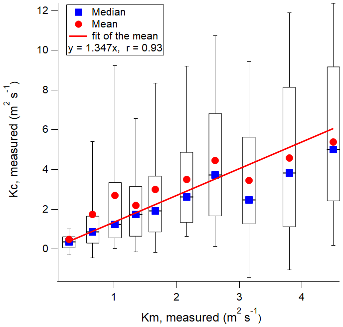
Figure 2 Calculating the Schmidt number Sc as a constant over the entire study. Lower and upper bounds of the box are the 25th and 75th percentile of each bin; the lines in the box and the blue squares mark the median; the red circle labels the mean of the data in each bin; whiskers are the 10th and 90th percentile of the data. In this analysis, measured K_c values were binned by K_m with 65 points in each bin. Bin centers were the median K_m measured of each bin. The red line is the best fit of mean K_c vs. median K_m of each bin. The p value of the fit = 0.0001. Points with K_m > 5 m² s⁻¹ were excluded in the fit.

The second approach is with variable Sc. Gualtieri et al.(2017) reviewed experimental and numerical simulation studies of the turbulent Schmidt number in the atmospheric environment and reported Sc values from 0.1 to 1.3. Flesch et al. (2002) measured the turbulent Sc of a pesticide in the atmosphere from soil emissions. Reported Sc in that study varied from 0.17 to 1.34 and showed that this was not solely due to measurement uncertainty. The Sc in this study also varies significantly over time when the wind is from the pond, from 0.04 to 2.90.

To investigate the real variability in Sc, $\mathit{Sc}=K_{\text{m\_measured}}/K_{\text{c\_measured}}$ was plotted against the stability parameter $z/L$ (Stull, 2003b), where L is the Obukhov length, for periods when the wind was from the pond direction (Fig. 3). Figure 3 shows that Sc becomes small as $z/L$ indicates increasingly unstable turbulent mixing, i.e., an increasing importance of convective (sensible heat driven) turbulence, which is not captured by an uncorrected K_m, vs. mechanical (momentum driven) turbulence. Sc varies significantly with $z/L$ and is associated with significant noise near neutral stability ($z/L$ close to 0). To avoid introducing large scatter in the Sc correction near neutral stability, Sc is set as 0.74 when $z/L$ is close to 0. To make the correction function continuous, a stepwise definition for Sc is given:

$$\begin{array}{}\text{(6)}& \mathit{Sc}=\left\{\begin{array}{ll}\mathrm{0.08}+\mathrm{3.13}\times {\mathrm{10}}^{-\mathrm{9}}{e}^{\left(\frac{\frac{z}{L}+\mathrm{19.5}}{\mathrm{1.008}}\right)},& \frac{z}{L}<-\mathrm{0.18}\\ \mathrm{0.74},& \frac{z}{L}\ge -\mathrm{0.18}.\end{array}\right.\end{array}$$

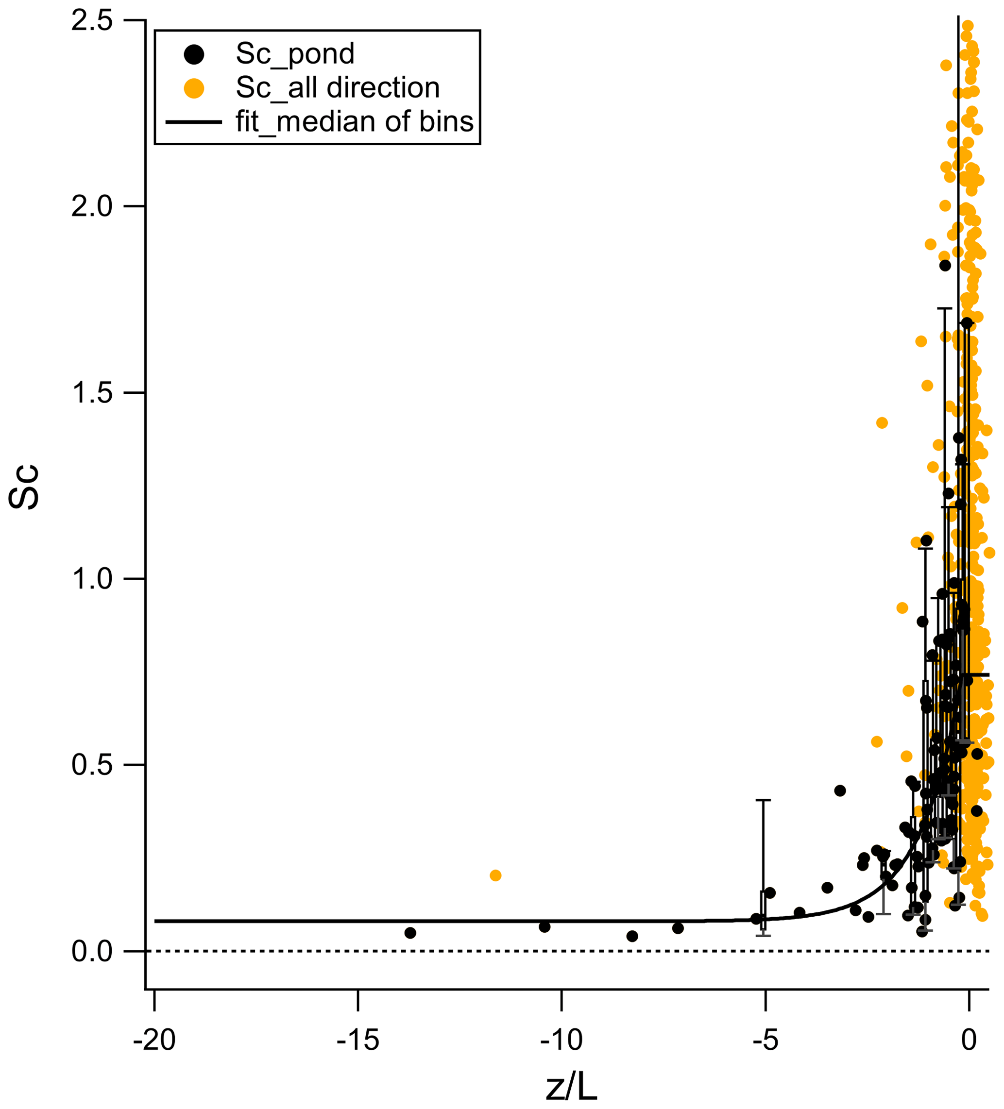
Figure 3 Dependence of Sc on $z/L$ measured at 18 m. Yellow points are Sc observed in each individual half-hour period over the entire period; black points are Sc observed in each individual half-hour period when the wind was from the pond; the black curve is the best fit of Sc versus median $z/L$ from each $z/L$ bin when the wind was from the pond. In this analysis, Sc was binned by $z/L$ with 10 points in each bin before fitting.

This Sc of the entire study period and a time series of $K_{\mathrm{c}}=K_{\mathrm{m}}/\mathit{Sc}$ (corresponding to 8 and 32 m measurements) were calculated. A three-point median smoothing was performed with the calculated K_c time series before the gradient flux of CH₄ was calculated using Eq. (3). To lessen the impact of extreme outliers, the final pond average fluxes reported were based on gradient fluxes between the 2.5th and 97.5th percentiles. In the Results and discussion section, gradient fluxes and plots from the variable Sc approach are shown, and results with the constant Sc approach are shown in Table S1 in the Supplement for comparison.

It is possible to calculate K_c values based on CO₂ in order to avoid potential circularity arguments when calculating gradient fluxes of CH₄ using this approach. However, the CO₂ flux signal from this pond was confounded by the strong natural variability of the CO₂ background, as well as the smaller signal-to-noise ratio of the pond CO₂ flux compared to the CH₄ flux (Fig. S1). Regardless, K_c values based on CO₂ were calculated and found to be noisier but statistically not different from those based on CH₄ (t test p = 0.09, based on fluxes binned into 16 wind direction sectors). It would also be possible to base the calculated K_c values on the sensible heat flux instead of the momentum flux, but due to the absence of significant heat fluxes at night, this would not provide the continuity that the momentum fluxes afford.

3.3 Inverse dispersion fluxes

Inverse dispersion models (IDMs) can be used to derive emission rate estimates based on line-integrated or point mole fraction measurements downwind of a defined source. Required inputs include the turbulence statistics between the source and point of observation. Unlike the EC and gradient techniques, IDMs also require an estimation of the background mole fraction of the pollutant upwind of the source. The backward Lagrangian stochastic (bLS) models are a specific subtype of IDMs. WindTrax 2.0 (Thunder Beach Scientific, http://www.thunderbeachscientific.com, last access: 26 January 2021; Flesch et al., 1995), based on a bLS model, is used in this study. The emission rate Q ($\mathrm{g}{\mathrm{m}}^{-\mathrm{2}}{\mathrm{d}}^{-\mathrm{1}}$) is calculated through

$$\begin{array}{}\text{(7)}& Q={\displaystyle \frac{(C-C_{\mathrm{b}})}{{\left(\frac{C}{Q}\right)}_{\text{sim}}}},\end{array}$$

where C [ppm] is the pollutant mole fraction at the measurement location, C_b is the background mole fraction of the pollutant, and $(C/Q{)}_{\text{sim}}$ is the simulated ratio of the pollutant mole fraction at the site to the emission rate from the specified source calculated by the bLS model. In this study, the meteorological condition inputs for the bLS model are u_∗ and L taken from the 30 min averaging calculation of ultrasonic anemometer measurements at 8 m, as well as 30 min average wind directions and ambient temperature directly from the propeller and temperature sensor at 4 m. Periods when $u_{\ast }<$ 0.15 m s⁻¹ were disregarded (Flesch et al., 2004). CH₄ mole fraction input was taken from the OP-FTIR measurement, which was located 10 m to the east of the flux tower. Emission rates are calculated by IDM only when the wind came from the pond, including the sectors centered at 270 and 90^∘.

3.4 Flux chamber measurements

Floating flux chamber measurements of CH₄ and CO₂ were conducted at 15 spots in and around bubbling zones, including 4 within 500 m of the tower, from 31 August to 2 September 2017, by Barr Engineering Co., using compliance monitoring procedures established with guidance from the Quantification of Area Fugitive Emissions at Oil Sands issued by Alberta Environment and Parks (AEP, 2019). On-site analysis of GHG was performed using U.S. Environmental Protection Agency (USEPA) flux chambers with real-time GHG analyzers (Los Gatos Research, Inc., USA). These flux chamber measurements were conducted during daytime. Key procedural steps include 45 min of purging pure nitrogen gas to reach an equilibrium between the flow of the inert carrier gas and the methane evolving from the pond surface, and measurement for a minimum of 30 min of with steady-state concentration readings. GHG gases reported from the chamber measurements include CH₄, CO₂, and N₂O (nitrous oxide). Fluxes were calculated according to the USEPA user's guide EPA/600/8-86/008 (USEPA 1986, Eqs. 3–5):

$$\begin{array}{}\text{(8)}& F_{\text{chamber}}={\displaystyle \frac{Q\cdot C}{A}},\end{array}$$

where Q is the flux chamber sweep air flow rate (L min⁻¹), A is the enclosed surface area (m²), and C is measured concentration (µg L⁻¹).

3.5 Area-weighted average of flux

To derive fluxes representing the whole pond, the half-hour fluxes (EC, gradient, and IDM fluxes) are binned by wind direction into 16 sectors. Area-weighted averages of fluxes for the pond F_pond are then calculated by

$$\begin{array}{}\text{(9)}& F_{\text{pond}}={\displaystyle \frac{\sum _{\text{sectors}}\stackrel{\mathrm{‾}}{F\left(\text{flux,\hspace{0.17em} sector}\right)}\cdot \text{Area\hspace{0.17em}(sector)}}{{\sum }_{\text{sectors}}\text{Area\hspace{0.17em}(sector)}}}.\end{array}$$

The area-weighted averages of flux results are summarized in Table 1 and serve as the final average fluxes representing the whole pond over the study period.

Table 1 Summary of CH₄ fluxes ($\mathrm{g}{\mathrm{m}}^{-\mathrm{2}}{\mathrm{d}}^{-\mathrm{1}}$) in this study.

^a Statistics and average fluxes are area weight averaged. ^b Statistics and average of 15 measurements described in Sect. 4.6. The error of the mean is the SD of the 15 measurements. Emission estimates were 5.3 $\mathrm{g}{\mathrm{m}}^{-\mathrm{2}}{\mathrm{d}}^{-\mathrm{1}}$ in 2016 and 11.1 $\mathrm{g}{\mathrm{m}}^{-\mathrm{2}}{\mathrm{d}}^{-\mathrm{1}}$ in 2018. ^c Errors with the mean fluxes are calculated with a top-down error estimation approach, using the average of SDs of fluxes from five periods when the fluxes displayed high stationarity.

4 Results and discussion

4.1 Meteorological conditions

As shown in the wind rose (Fig. S2 in the Supplement), wind coming from the pond occurred only about 22 % of the entire measurement period. The dominance of winds from the background directions was known before the study, based on records from monitoring stations in the area, but logistical and access constraints limited us to using the south shore for the setup. There was no significant diurnal variation in wind direction over the entire period. The ambient temperature during the measurement period varied from 7.5 to 31.1 ^∘C, with an average of 17.5 ^∘C (Fig. 4b). The mean wind speed measured with the propeller anemometer at 4 m was 3.0 m s⁻¹, with a range from 0 to 14.9 m s⁻¹, and quartiles of 1.7 and 4.0 m s⁻¹ (Fig. 4a). The mean friction velocity at 8 m (the lowest height by sonic anemometer measurement) over the whole measurement period was 0.32 m s⁻¹ (Fig. 4a), with a range from 0.03 to 1.01 m s⁻¹ and quartiles are 0.20 and 0.42 m s⁻¹. Wind speed and friction velocity had a predictable diurnal pattern: greater during the day than at night (Fig. 4a).

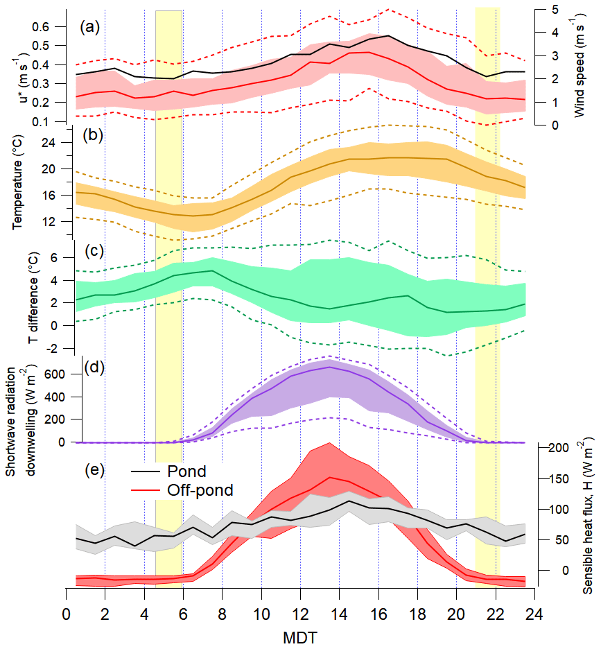
Figure 4 Diurnal variations of (a) u_∗ at 8 m (red) and wind speed at 4 m (black); (b) ambient temperature at 8 m; (c) the temperature difference between the surface of the pond and the ambient temperature at 8 m; (d) downwelling shortwave radiation; (e) the sensible heat flux at 8 m. Solid lines show the median, shades indicate the interquartile ranges, and dashed lines label the 10th and 90th percentiles. MDT denotes mountain daylight savings time (hours). The yellow shades mark the range of local sunrise and sunset times during this 5-week project.

In Fort McMurray during the study period, the sunrise was in the range of 04:35 to 05:56 MDT (mountain daylight savings time, UTC−6), solar noon occurs at around 13:30 and sunset occurs in the range of 22:25 to 20:49 MDT (Fig. 4d). Winds across the pond and from the south pass over markedly different surface types (liquid pond vs. a mixture of solid surface types), so the sensible heat flux H is analyzed separately based on the wind direction (Fig. 4e). During the day (from 08:00 to 19:00), H associated with winds across the pond was consistently smaller than H with winds from other directions, suggesting the pond absorbs significant solar energy at the site during the day. It is also worth mentioning that H stayed positive during the night when the wind came across the pond, consistent with the observation that the pond surface temperature was greater than the air temperature (Fig. 4c). These resulted in convective turbulent transport of species emitted from the pond surface throughout the night.

4.2 Footprint of flux measurements

The footprint of a micrometeorological flux measurement, i.e., the area upwind that contributes to the flux at the point of observation, depends on the wind speed and the dynamic stability of the surface layer. The footprints of EC fluxes measured at 18 m at each half-hour period were estimated using the algorithm by Kljun et al. (2015), which takes mean wind speed, boundary layer height, wind direction, friction velocity, Obukhov length, and SD of horizontal wind speed. Boundary layer height was estimated using the lidar measurements at Fort McKay in August 2017 (Strawbridge et al., 2018). Footprints under unstable conditions are summarized in the polar plot in Fig. 1. Footprint contribution distances were calculated for each half hour over the entire period of study. Results were further separated into unstable ($z/L\le -\mathrm{0.0625}$), neutral (−0.0625 < $z/L$ < 0.0625), and stable ($z/L\ge \mathrm{0.0625}$) conditions. Since unstable conditions applied 98.6 % of time when the wind was from the pond and 52 % of entire measurement period, we summarized the unstable condition footprint results into 16 wind direction bins, and medians are shown in the polar plot in Fig. 1 (footprint under neutral and stable conditions is shown in Fig. S3 in the Supplement). The footprint results show the EC flux footprint lies mostly within the edges of the pond.

For gradient flux measurements, the effective footprint is the same as the EC footprint at the geometric mean of the two sample heights (Horst, 1999) for a homogeneous surface area upwind. In this study, gradients between 8 and 32 m therefore have a footprint equivalent to that for EC at 16 m, reasonably close to where the 18 m EC fluxes were measured. Since the concentration footprint at the upper (32 m) level is larger than the concentration footprint at the lower (8 m) level, the gradient flux may be affected by sources beyond the geometric mean footprint.

4.3 Eddy covariance flux

Analysis of CH₄ mole fractions at 18 m as shown in Fig. 5 clearly indicates that CH₄ was elevated when the wind was from the pond direction, and it was steady at round 1.9 ppm when the wind was from other directions (Figs. 5 and 6). Besides sectors from the pond directions, Fig. 7 shows CH₄ fluxes significantly larger than zero from two sectors centered with 90 and 270^∘, i.e., along the shorelines to the east and west. Therefore, measured results for air coming from these two sectors could represent a mixture of air carrying pond emissions and air from the shore. EC fluxes from the four wind direction sectors centered in the range of 292.5 to 0^∘ are close to each other.

Figure 5 Rose plot of CH₄ mole fraction at 18 m. Colors represent CH₄ mole fraction. The length of each colored segment represents the time fraction of that mole fraction range in each direction bin. The radius of the black open sectors indicates the frequency of wind in each direction bin; the angle represents wind direction.

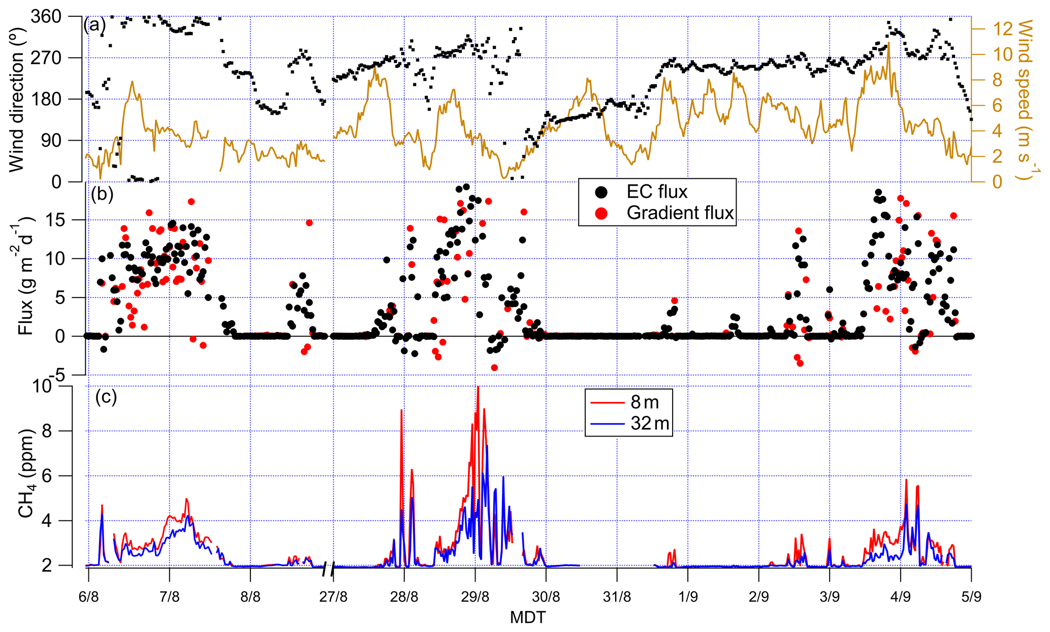
Figure 6 Time series of (a) wind direction and wind speed, (b) CH₄ EC fluxes and gradient fluxes, and (c) CH₄ mole fractions at 8 and 32 m, from 6 to 9 August and from 27 August to 5 September.

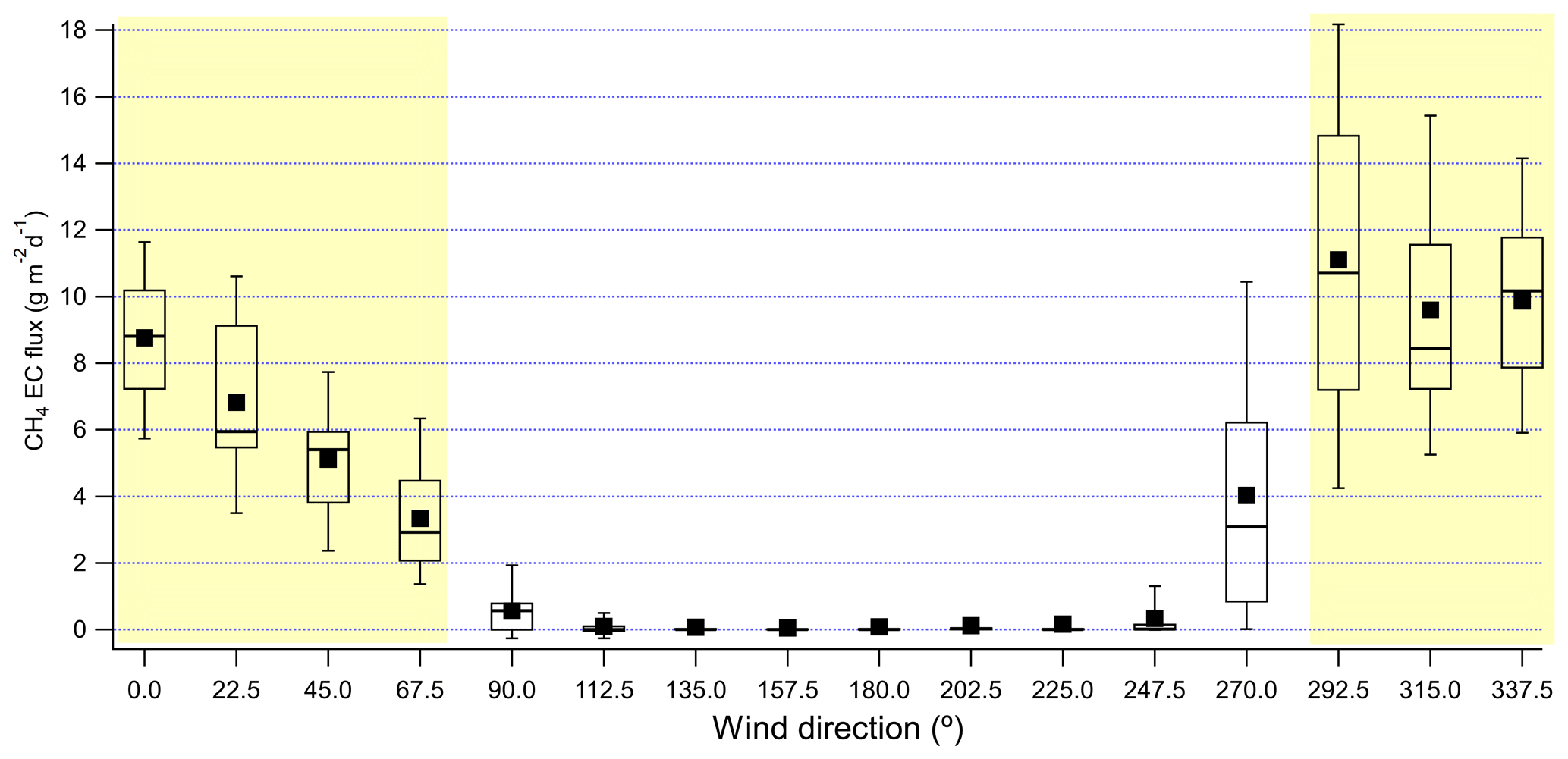
Figure 7 EC flux of CH₄ as a function of wind direction binned in 22.5^∘ bins. Lower and upper bounds of the box plot are the 25th and 75th percentile; the line in the box marks the median and the black square labels the mean; the whiskers label the 10th and 90th percentile. Yellow shades indicate the wind directions from the pond.

There was no statistically significant diurnal pattern of the CH₄ EC flux when the wind came from the pond direction (WD ≥ 286^∘ or WD ≤ 76^∘) (relative SD is 15 %, p=0.54) (Fig. S4a in the Supplement). The diurnal pattern of another three sectors when the wind was not from the pond were studied. The sector 259^∘ ≤ WD < 286^∘ (Fig. S4b) contains a mixture of pond emission and the shore of the pond, and it also showed no significant diurnal pattern. The sector 214^∘ ≤ WD < 259^∘ (Fig. S4c) mainly covers trees and a lake and showed a slightly increased flux during 12:00–18:00, which is likely due to biogenic emission from trees and soils (Covey and Megonigal, 2019). The sector 124^∘ ≤ WD  < 146^∘ (Fig. S4d) covered a workers' lodge and parking lots, and CH₄ emissions and diurnal variation were close to zero. The lack of a diurnal variation of CH₄ EC flux observed when the wind was from the pond in this study was similar to the lack of diurnal variation of CH₄ EC flux at another tailings pond reported by Zhang et al. (2019).

Relationships between the flux when the wind was from the pond and various meteorological parameters were investigated, and results show that fluxes showed a weak dependence on wind speed, u_∗, water surface temperature, or the temperature difference between the water surface and 8 m (Fig. S5 in the Supplement); i.e., they were not major drivers of the CH₄ emission rate. CH₄ at this site is mainly produced through the methanogenesis of hydrocarbon by the microbes in the fine tailings covering a range of depth in the pond (Penner and Foght, 2010; Siddique et al., 2011, 2012) and therefore is not directly affected much by the meteorological conditions at the surface or above the pond.

4.4 CH₄ gradient flux and comparison with EC flux

The CH₄ mole fraction measured at 8 and 32 m shows that winds across the pond carried significantly more CH₄ than from other directions, and there was a clear vertical gradient with mole fraction at 8 m on the order of 0.5 ppm or more higher than at 32 m (Fig. 6). Gradient fluxes were calculated for all periods when valid EC fluxes and concentration gradients were available. The gradient flux derived from measurements at 8 and 32 m shows that the flux was minimal when the wind was from other directions, similar to the EC flux (Fig. S6 in the Supplement). Due to significant scatter, the half-hour gradient fluxes were statistically different from the EC fluxes when the wind was from the pond direction (p=0.003). They were moderately correlated (slope = 0.80, r=0.32, Fig. S7a in the Supplement). To obtain some comparability, it is therefore necessary to average blocks of data into appropriate bins. A t test of the gradient and eddy average fluxes binned by wind direction (22.5^∘ blocks) yielded a p=0.30, and hourly diurnal averaged fluxes agreed with a p=0.09. The pond-area-weighted mean gradient flux was 8 % lower than EC flux, and the median was 18 % less than EC flux (Table 1).

Studies comparing MBR and EC CH₄ fluxes are rare. Zhao et al. (2019) compared CH₄ fluxes from an MBR method as well as from an aerodynamic flux model to EC fluxes for two small fish ponds and showed that the MBR fluxes were well correlated with EC fluxes, with a mean 27 % greater than the EC mean flux. The gradient flux calculation in our study can be considered a hybrid of the MBR and aerodynamic methods, based on a continuous time series of eddy diffusivities for momentum, scaled by the eddy diffusivity for CH₄. The gradient fluxes of CH₄ agreed well with EC flux in our study, providing a basis for applying the derived K_c values to calculate gradient fluxes for a variety of other gases emitted by the pond (e.g., You et al., 2021). Other studies comparing MBR with eddy covariance methods on other gases fluxes, such as CO₂, have been reported. Xiao et al. (2014) showed that fluxes of CO₂ from these two methods were comparable at Lake Taihu. Wolf et al. (2008) and Bolinius et al. (2016) used EC of heat to derive gradient fluxes of CO₂ over trees and showed they were comparable with EC fluxes.

Gradient fluxes were also calculated with the constant Sc approach, as described in Sect. 3.2, and results are listed in Table S1. Gradient fluxes calculated from a constant Sc were significantly lower than gradient fluxes with the variable Sc approach ($p<{\mathrm{10}}^{-\mathrm{21}}$; the pond average mean (median) is 33 % (34 %) lower, respectively). Results from this study clearly present the variable nature of Sc and that correcting Sc with stability ($z/L$) is effective to improve gradient flux calculations. While the function derived (Eq. 6) is primarily a function of the characteristics of atmospheric turbulence and should have broad applicability, it is based on a limited data set and should be verified in other settings in future studies.

4.5 CH₄ inverse dispersion flux and comparison with EC flux

Compared to point measurements, path-integrated measurements have the advantage of being less sensitive to changes in wind direction and being representative of larger areal averages (Flesch et al., 2004). Therefore, the bottom path-integrated CH₄ mole fraction of the FTIR was used as input for the IDM flux estimate. The bottom path measurement had the greatest signal-to-noise ratio and a footprint on the order of 1–2 km, which is comparable to the footprint of the EC and gradient fluxes (Fig. 1). CH₄ IDM flux calculated from the path-integrated mole fraction inputs from OP-FTIR bottom path measurements (when the OP-FTIR path was downwind of the pond) compared well to EC flux, based on the set of simultaneous half-hour periods when both EC and IDM fluxes were available. IDM and EC flux showed reasonable correlation (r=0.62) with a slope of 0.69 (Fig. S7b), although the averaged half-hour IDM fluxes are significantly different from EC fluxes ($p<{\mathrm{10}}^{-\mathrm{4}}$). Binning into 16 wind direction sectors similar to that described in Sect. 4.4 yielded agreement at the p=0.08 level. The pond-area-weighted mean IDM flux was 30 % smaller than EC flux, and the pond-area-weighted median IDM flux was also 30 % smaller than EC median flux. Some of the differences are likely due to the different footprints of the two measurements. The footprint for turbulent fluxes is smaller than the footprint for concentrations at the same height (Schmid, 1994). The IDM flux showed weak diurnal variations when the wind came from the pond directions (Fig. S8 in the Supplement), with smaller fluxes during the day compared to fluxes at night (p=0.04) – inconsistent with EC and gradient fluxes. As stated in Sect. 3.3, half-hour periods when u_∗ < 0.15 m s⁻¹ were excluded in IDM calculation (Flesch et al., 2004). This filtering excluded more nighttime fluxes than daytime fluxes, which caused more limited data in IDM nighttime fluxes and biased the t test.

Since the background mole fraction input for IDM calculation could affect the flux estimates, two approaches to determining background mole fraction of CH₄ for model inputs were tested: the daily minimum of CH₄ from wind sectors between 180 and 240^∘ of OP-FTIR at our site; the CH₄ from another independent OP-FTIR measurement on the north shore of this pond (details are described in You et al., 2021). Results of IDM fluxes with these two background approaches agreed well (You et al., 2021).

4.6 Flux chamber measurements

Fluxes from the 15 flux chamber measurements over 3 d in and around the bubbling zones varied from 0.9 to 5.1 $\mathrm{g}{\mathrm{m}}^{-\mathrm{2}}{\mathrm{d}}^{-\mathrm{1}}$, with an average of 2.8 $\mathrm{g}{\mathrm{m}}^{-\mathrm{2}}{\mathrm{d}}^{-\mathrm{1}}$ and a median of 2.3 $\mathrm{g}{\mathrm{m}}^{-\mathrm{2}}{\mathrm{d}}^{-\mathrm{1}}$. The average flux of the five measurements on the last day, 2 September, is 3.6 $\mathrm{g}{\mathrm{m}}^{-\mathrm{2}}{\mathrm{d}}^{-\mathrm{1}}$, which is the highest amongst the 3 d. The great variation amongst these 15 measurements shows the pond was highly heterogeneous in terms of CH₄ emissions. The average fluxes from these flux chamber measurements are about half of the average fluxes from the EC, gradient, and IDM methods. While the flux chamber measurements were deployed over the three days, the wind was from the south, so no simultaneous comparison could be made between flux chamber measurements and micrometeorological methods. However, based on the micrometeorological fluxes spanning more than a month, there is no evidence of day-to-day variability of this magnitude, and we conclude that the mismatch is due to spatial or methodological differences.

Annual compliance flux chamber measurements in 2016 resulted in pond average fluxes of 5.3 and 11.1 $\mathrm{g}{\mathrm{m}}^{-\mathrm{2}}{\mathrm{d}}^{-\mathrm{1}}$ in 2018, despite similar operational parameters in these years as in 2017. We conclude that the underestimate in 2017 is not an indication of a systematic bias of flux chambers but rather a measure of the uncertainty involved in flux estimates based on snapshot chamber measurements.

A few other studies have also discussed differences between flux chambers and micrometeorological methods (Schubert et al., 2012; Podgrajsek et al., 2014; Erkkilä et al., 2018; Zhang et al., 2019). Zhang et al. (2019) measured CH₄ emission from another tailings pond and reported flux chamber measurements were more than 10 times greater than fluxes from the EC method. They stated that strong eruptions of bubbles could overwhelm the chamber and result in a local underestimation of the flux. On the other hand, the lower EC flux estimate suggests that the area average flux was being overestimated by extrapolation from the chambers, which may have preferentially been located over bubble zones. Their EC fluxes were 2 orders of magnitude smaller than CH₄ flux in this study. Results from this study and Zhang et al. (2019) suggest that average tailings pond CH₄ emission extrapolated from a few individual flux chamber measurements may significantly underestimate or overestimate fluxes relative to area-averaging micrometeorological measurements.

This has also been shown over other water surfaces. Podgrajsek et al. (2014) investigated CH₄ fluxes at the lake Tämnaren and reported the fluxes from the EC and flux chamber were on the same order of magnitude. They stated that due to the non-continuous measurement of flux chambers, some high-flux short episodes could be missed. Schubert et al. (2012) measured CH₄ fluxes from lake Rotsee and reported the fluxes from the EC and flux chamber compared well. Erkkilä et al. (2018) measured CH₄ flux at Lake Kuivajärvi with the two methods when the lake was stratified and reported flux chamber measurements were significantly greater than EC fluxes. In conclusion, while flux chambers present advantages in terms of finer spatial and temporal resolution for small sources or locations with high spatial heterogeneity, reliance on a limited number of flux chamber measurements can result in significant year-to-year variability, and spatially integrating methods such as eddy covariance or gradient fluxes will generally provide more representative averages.

Table 2 Comparison of CH₄ fluxes ($\mathrm{g}{\mathrm{m}}^{-\mathrm{2}}{\mathrm{d}}^{-\mathrm{1}}$) in this study to previously reported fluxes.

^a The original units are $\mathrm{t}{\mathrm{ha}}^{-\mathrm{1}}{\mathrm{yr}}^{-\mathrm{1}}$. Measurements were taken from August to October in 2010 or 2011. The pond area was 2.8 km² as listed in Table 1 of Small et al. (2015). We assumed no seasonal variations to extrapolate from summer measurements to annual totals. ^b The original number is 2.0 t h⁻¹, and the pond water surface area used was 2.8 km² (Small et al., 2015). BDL: below detection limit. NA: not available.

4.7 Comparison with previous results

Emissions reported in Small et al. (2015) and a Stantec report (2016) (Table 2) represent estimates extrapolated from individual flux chamber measurements and did not incorporate any seasonal variations for microbial CH₄ emissions. Therefore, to compare result of this study to results summarized in Small et al. (2015), we simply used 1 year = 365 equal days. Small et al. (2015) showed that CH₄ emissions from the same pond were 2.6 $\mathrm{g}{\mathrm{m}}^{-\mathrm{2}}{\mathrm{d}}^{-\mathrm{1}}$ based on the averaging of flux chamber measurements during August to October in 2010 and 2011. A Stantec compliance report (2016) presented flux chamber measurements on this pond with resulting average fluxes of 12.9 and 2.1 $\mathrm{g}{\mathrm{m}}^{-\mathrm{2}}{\mathrm{d}}^{-\mathrm{1}}$ (bubbling and quiescent zones, respectively) in 2013 and 9.6 $\mathrm{g}{\mathrm{m}}^{-\mathrm{2}}{\mathrm{d}}^{-\mathrm{1}}$ and below the detection limit, respectively, in 2014. EC fluxes of CH₄ in this study are a factor of 2.8 greater than flux chamber measurements which were taken during the last few days of this project and a factor of 3 greater than emissions reported in Small et al. (2015). However, CH₄ fluxes in this study are 19 % to 40 % smaller than the fluxes from the bubbling zones in 2013 and 2014 (Stantec, 2016). The big differences between flux chamber measurements in the bubbling and quiescent zones may suggest micrometeorological measurements with a bigger footprint will perform better in quantifying emission from the whole pond. It is worth noting that the seasonal variation of fugitive emission from tailings pond is still not well understood and that different daily emissions are derived from the tabulated annual results from Small et al. (2015) depending on the annual extrapolation model used. This reflects a general complication when comparing the 5-week emission results in this study to annual emissions reported in the past.

Baray et al. (2018) calculated CH₄ emission from this pond based on airborne measurement in 2013 over the whole facility, combined with reported statistics stating that 58 % of CH₄ emissions within the facility were from tailings ponds, and 85 % of emissions from these tailings ponds were from Pond $\mathrm{2}/\mathrm{3}$. This resulted in an estimate of 2.0 ± 0.3 t h⁻¹, which converts to 17.1 $\mathrm{g}{\mathrm{m}}^{-\mathrm{2}}{\mathrm{d}}^{-\mathrm{1}}$ (for a pond area of 2.8 km², Small et al., 2015, Table 2). This emission rate is significantly (119 %) greater than emissions from the three micrometeorological methods in this study, possibly because of the uncertainties in the reported percentage contribution of CH₄ emissions from this pond to the whole facility.

Suncor reported facility-wide emissions of CH₄ for 2017 of 5977 t (Government of Canada, 2017). The emissions measured during the 5 weeks of this study extrapolated to the year result in 6548 t yr⁻¹, i.e., 110 % of this total. This extrapolation assumes seasonal invariance of CH₄ emissions (e.g., January emissions are the same as August emissions) as is common practice in monitoring reports (cf. Stantec, 2016).

When comparing CH₄ emissions in this study to emissions summarized in Table 2, it must be kept in mind that different time periods are being compared and that several factors may contribute to variability of the emissions (Siddique et al., 2007, 2012). Pond $\mathrm{2}/\mathrm{3}$ is an active pond, and the amount and characteristics of input streams are variable with time. Some of the facility-specific variables which could affect the methane emissions include the amount of diluent loss to the pond, the proportions of diluent and hydrocarbons in the froth treatment tailings (FTT) that enter matured fine tailings (MFT) layers in the pond, density of microbes in the MFT, physical disturbance of the MFT layers, transferring activities of the MFT, pond water temperature change and consequential density inversion between oil layers and water in the pond, FTT discharge diluent composition change, introduction of new materials and chemicals into the MFT, and consequential change in microbial community (Small et al., 2015; Foght et al., 2017). Natural lakes and wetlands emit at rates typically on the order of 0.005–0.05 $\mathrm{g}{\mathrm{m}}^{-\mathrm{2}}{\mathrm{d}}^{-\mathrm{1}}$ (Sanches et al., 2019). Another independent approach to estimating CH₄ emissions is using an emission factor (EF) combined with diluent discharge rates to the pond. The EF was based on an MFT characterization and kinetics of methanogenesis for a matured pond. Pond $\mathrm{2}/\mathrm{3}$ is presumably similar in maturity and properties to the studied MFT in other oil sands facility (Siddique et al., 2008). After incorporating the diluent loss to the pond, the daily CH₄ emissions were calculated and integrated into an annual emission of 5860 t, which is comparable to annual emissions extrapolated from the micrometeorological methods in this study. This approach requires some assumptions: first, that the kinetics of methanogenesis are a function of the maturity of the microbial community within the target MFT; and, second, that the properties of the diluent feed stream remain constant over the period considered. This approach can provide emission estimates continually, provided that the microbial state in the MFT and the diluent discharge volumes and properties are tracked and remain consistent.

To put the CH₄ emissions into a global warming context, the CH₄ fluxes can be combined with concurrent flux measurements of CO₂ with the same instrumentation. Assuming a GWP of CH₄ = 28 (Myhre et al., 2013), the equivalent CO₂ flux ($F_{{\mathrm{CO}}_{\mathrm{2}\mathrm{eq}}}$) from this tailings pond $F_{{\mathrm{CO}}_{\mathrm{2}\mathrm{eq}}}$ = $F_{{\mathrm{CO}}_{\mathrm{2}}}$ + $(F_{{\mathrm{CH}}_{\mathrm{4}}}\cdot \text{GWP})$ = 204 kt yr⁻¹, 90 % of which is due to CH₄. This accounts for only 3 % of Suncor's facility CO_2eq emissions in 2017 due to the dominance of other CO₂ sources.

5 Conclusions

Results in this study have provided several estimates of the emission of CH₄ from this tailings pond using EC, gradient, and IDM for a period of 5 weeks. The gradient and inverse dispersion methods agreed moderately with EC results (18 % and 30 % lower, respectively), which lends confidence that the former two methods can provide valid flux estimates for other gases emanating from the pond. These results were also compared to flux chamber measurements at this pond taken during the study, showing flux chamber estimates were 64 % lower than those from micrometeorological methods. The better agreement between the three micrometeorological measurements flux results suggests that the larger footprint of micrometeorological measurements results in more robust emission estimates representing most of the pond area. Fluxes were shown to have only a minor diurnal cycle, with a 15 % variability, during the period of this study. To investigate seasonal patterns, further studies measuring CH₄ fluxes using micrometeorological methods at this pond or other tailings ponds throughout the year are recommended.