A new method to detect and classify polar stratospheric nitric acid trihydrate clouds derived from radiative transfer simulations and its first application to airborne infrared limb emission observations

Polar stratospheric clouds (PSCs) play an important role in the spatial and temporal evolution of trace gases inside the polar vortex due to different processes, such as chlorine activation and NO_y redistribution. As there are still uncertainties in the representation of PSCs in model simulations, detailed observations of PSCs and information on their type – nitric acid trihydrate (NAT), supercooled ternary solution (STS), and ice – are desirable.

The measurements inside PSCs made by the CRISTA-NF (CRyogenic Infrared Spectrometers and Telescope for the Atmosphere – New Frontiers) airborne infrared limb sounder during the RECONCILE (Reconciliation of essential process parameters for an enhanced predictability of Arctic stratospheric ozone loss and its climate interactions) aircraft campaign showed a spectral peak at about 816 cm⁻¹. This peak is shifted compared with the known peak at about 820 cm⁻¹, which is recognised as being caused by the emission of radiation by small NAT particles. To investigate the reason for this spectral difference, we performed a large set of radiative transfer simulations of infrared limb emission spectra in the presence of various PSCs (NAT, STS, ice, and mixtures) for the airborne viewing geometry of CRISTA-NF. NAT particles can cause different spectral features in the 810–820 cm⁻¹ region. The simulation results show that the appearance of the feature changes with an increasing median radius of the NAT particle size distribution, from a peak at 820 cm⁻¹ to a shifted peak and, finally, to a step-like feature in the spectrum, caused by the increasing contribution of scattering to the total extinction. Based on the appearance of the spectral feature, we defined different colour indices to detect PSCs containing NAT particles and to subgroup them into three size regimes under the assumption of spherical particles: small NAT (≤ 1.0 µm), medium NAT (1.5–4.0 µm), and large NAT (≥ 3.5 µm). Furthermore, we developed a method to detect the bottom altitude of a cloud by using the cloud index (CI), a colour ratio indicating the optical thickness, and the vertical gradient of the CI. Finally, we applied the methods to observations of the CRISTA-NF instrument during one local flight of the RECONCILE aircraft campaign and found STS and medium-sized NAT.

1 Introduction

Polar stratospheric clouds (PSCs) form inside the cold polar vortices in both hemispheres in winter. They have a major influence on the ozone chemistry and, thus, ozone depletion in the stratosphere (Solomon, 1999). PSCs are classified into three different types: supercooled ternary solution (STS) droplets, nitric acid trihydrate (NAT), and ice particles (e.g. Lowe and MacKenzie, 2008). The formation and existence of these different types is largely temperature dependent. Solid ice particles can only exist below the frost point T_frost ≈ 188 K, whereas NAT particles are thermodynamically stable at temperatures below T_NAT ≈ 195 K. The liquid STS droplets form from binary H₂SO₄–H₂O droplets at temperatures below the dew point of HNO₃ T_dew ≈ 192 K by the uptake of HNO₃ (see e.g. Peter and Grooß, 2012, and references therein).

PSCs directly and indirectly influence the spatial distribution of trace gases relevant for ozone depletion in different ways. Due to heterogenous reactions on the cold particle surfaces, chlorine is activated from its reservoir species, mainly HCl and ClONO₂, and the chlorine radicals catalytically destroy ozone (e.g. Solomon, 1999). NAT particles can grow to larger sizes, which then leads to a sedimentation of the particles and, thus, to a permanent removal of HNO₃ from the stratosphere (denitrification) (e.g. Fahey et al., 2001; Molleker et al., 2014). This denitrification slows down the deactivation of chlorine and, therefore, enhances the ozone loss (e.g. Waibel et al., 1999; Peter and Grooß, 2012).

Because of these different processes and due to the fact that many models rely on rather simple parameterisations, the simulation of PSCs and related processes is incomplete and is also partly accompanied by larger uncertainties. Specifically, chemistry climate models (CCMs) that are used to assess polar stratospheric ozone loss (e.g Eyring et al., 2013) often employ rather simple schemes to represent PSCs in the model simulations. Such simplifications may lead to a heterogeneous chemistry dominated by NAT, but it is known that heterogeneous chemistry on STS and cold binary aerosol particles probably dominates the chlorine activation (e.g Solomon, 1999; Drdla and Müller, 2012; Kirner at al., 2015). Additionally, no comprehensive microphysical models are typically used to describe the evolution of PSCs over the winter. Mesoscale temperature variations that are known to play an important role in the formation of PSCs (Carslaw et al., 1998; Dörnbrack et al., 2002; Engel et al., 2013; Hoffmann et al., 2017) are also missing in current state-of-the-art CCMs (Orr et al., 2015).

Assumptions regarding the occurrence of different PSC types typically only have a limited impact on many aspects of ozone loss, as, for example, liquid PSC particles are sufficient to simulate nearly all ozone loss (Wohltmann et al., 2013; Kirner at al., 2015; Solomon et al., 2015). However, there are also situations where the PSC type is crucial. For example, the specific PSC type present at the top of the ozone loss region is important (Kirner at al., 2015), and type also plays an important role during the initial activation in PSCs covering only a small part of the vortex (Wegner et al., 2012). Furthermore, the heterogenous reaction rates on PSCs strongly depend on temperature as well as on the PSC type (e.g. Drdla and Müller, 2012; Wegner et al., 2012). Here, especially for NAT, the reaction rates show rather large uncertainties (Carslaw et al., 1997; Wegner et al., 2012), which highlights the importance of observing the PSC type.

In summary, information on the composition of PSCs is very important, but measurements are limited. Typical PSC measurement techniques are in situ particle measurements and lidar observations (e.g. Molleker et al., 2014; Achtert and Tesche, 2014; Pitts et al., 2018). However, in addition to these above-mentioned measurement techniques, an infrared limb emission sounder builds a good basis for PSC studies (e.g. Spang and Remedios, 2003; Höpfner et al., 2006).

In addition to the derivation of volume mixing ratios of several trace gases, infrared limb emission sounders such as CRISTA (CRyogenic Infrared Spectrometers and Telescopes for the Atmosphere; Offermann et al., 1999; Grossmann et al., 2002), CRISTA-NF (CRyogenic Infrared Spectrometers and Telescope for the Atmosphere – New Frontiers; Kullmann et al., 2004), and MIPAS-Envisat (Michelson Interferometer for Passive Atmospheric Sounding – Envisat; Fischer et al., 2008) are well-suited to detect clouds of different composition. Spang et al. (2001) established a simple and effective cloud detection method based on the radiance ratio of two specific spectral regions. The first one is dominated by CO₂ molecular line emissions (around 792 cm⁻¹), and the second one is dominated by the broader continuum-like aerosol emissions (around 833 cm⁻¹). This detection method was then successfully used in various studies and for different satellite and airborne instruments (e.g. Spang and Remedios, 2003; Spang et al., 2002, 2005, 2008, 2015; Höpfner et al., 2006; Kalicinsky et al., 2013). Furthermore, the infrared spectra exhibit different spectral features or radiance behaviours in the presence of different types of polar stratospheric clouds. Spang and Remedios (2003) presented a sharp peak-like feature at around 820 cm⁻¹ observed by the CRISTA instrument in the Antarctic winter for the first time. They attributed this feature to HNO₃-containing particles. Höpfner et al. (2006) showed that the feature can be best reproduced in simulations by using refractive index data for β-NAT particles (assuming relatively high number densities). The authors showed that the colour ratio method derived by Spang and Remedios (2003) that exploits the peak-like feature for detection is able to identify PSCs containing small NAT particles (radii < 3 µm). By means of a large set of radiative transfer simulations, Spang et al. (2012, 2016) developed a detection and discrimination method for PSCs. Besides the feature at 820 cm⁻¹, the method also uses further spectral behaviours such as a radiance decrease from around 830 cm⁻¹ towards larger wavenumbers (around 950 cm⁻¹) that occurs in the case of ice to distinguish different PSC types. Spang et al. (2018) finally presented a climatology of the PSC composition for the whole MIPAS-Envisat observation time period (2002–2012) based on this method.

During the RECONCILE campaign (Reconciliation of essential process parameters for an enhanced predictability of Arctic stratospheric ozone loss and its climate interactions; von Hobe et al., 2013) a slightly different type of spectral feature was observed by the CRISTA-NF infrared limb emission sounder in the presence of PSCs. The campaign took place in Kiruna, Sweden, from January to March 2010, and the high-flying M55-Geophysica research aircraft carried out a number of flights with a huge set of different instruments in order to study the polar vortex and related scientific topics, such as PSCs, ozone chemistry, and mixing processes. CRISTA-NF was one of the instruments operated and is able to detect clouds and distinguish different types of PSCs. During the first five flights of the campaign (17–25 January 2010), CRISTA-NF detected PSCs around the aircraft. Because of the viewing geometry of an infrared limb sounder, where the horizontal distance of a tangent point to the aircraft increases with decreasing sampling altitude, CRISTA-NF typically observes air masses in a wider range around the aircraft. The infrared spectra measured inside the clouds show a noticeable spectral feature at about 816 cm⁻¹. This feature is slightly shifted towards smaller wavenumbers compared with the typical spectral feature at 820 cm⁻¹, which is caused by very small NAT particles. Another appearance of the spectral feature caused by NAT particles, a step-like or shoulder-like behaviour of the radiance in the 810–820 cm⁻¹ spectral region, was observed by the MIPAS-B balloon-borne instrument in January 2001 (Höpfner et al., 2002) and the MIPAS-STR airborne instrument during the ESSENCE campaign in December 2011 (Woiwode et al., 2016). Woiwode et al. (2016) analysed different particle modes with radii between 1 and 6 µm and suggested that highly aspherical medium to large-sized (median radius 4.8 µm) NAT particles caused the change in the NAT signature to the step-like appearance. Woiwode et al. (2016) concluded that the particle shape and the scattered radiation from below can influence the feature. However, the appearance of the spectral feature seems to depend on the particle size distributions of the NAT particles, especially on the median radius. This motivated the following study of the relationship between the appearance of the feature (typical, shifted, and step-like) and the corresponding particle size distribution, aiming at an improved detection method for PSCs containing NAT particles. In particular, the possibility to detect larger NAT particles is important, because they play a major role in the denitrification of the stratosphere (Fahey et al., 2001; Molleker et al., 2014) and, thus, in ozone chemistry as a whole (e.g. Waibel et al., 1999; Peter and Grooß, 2012). New insights and an improvement in the detection method are also interesting for measurements of other infrared limb emission sounders such as MIPAS-Envisat, where data for a long observation period (about 10 years) and both hemispheres are available. For this purpose, a large variety of different PSCs with respect to the composition, spatial dimensions, and particle size distributions of the PSC particles were simulated and analysed.

The paper is structured as follows: in Sect. 2, the CRISTA-NF instrument and the radiative transfer code are described, and the set-up used for the simulations is explained; the results of the simulations are presented and analysed in Sect. 3; the derived methods are applied to the CRISTA-NF measurements in Sect. 4; and, finally, the main results are discussed in Sect. 5 and summarised in Sect. 6.

2 Methods and set-up

The radiative transfer simulations were performed using the viewing geometry and spectral properties of the CRISTA-NF airborne infrared limb sounder. The background atmosphere used for the simulations is a polar winter atmosphere with conditions suitable for the formation of polar stratospheric clouds. The simulations themselves were performed using the Juelich Rapid Spectral Simulation Code (JURASSIC). This section describes the CRISTA-NF instrument, the JURASSIC radiative transfer code, the set-up used for the simulations, and the different cloud scenarios that were investigated.

2.1 CRISTA-NF instrument

The airborne CRISTA-NF instrument is a successor of the CRISTA satellite instrument. CRISTA-NF measures the thermal emissions of the atmosphere in the mid-infrared region from 4 to 15 µm in an altitude range from flight altitude (up to 20 km) down to approximately 5 km. A detailed description of the design of the cryostat and the optical system is given by Kullmann et al. (2004). The calibration procedure and some improvements for the RECONCILE campaign are described by Schroeder et al. (2009) and Ungermann et al. (2012) respectively.

CRISTA-NF uses a Herschel telescope and a tiltable mirror to scan the atmosphere from flight altitude down to approximately 5 km. The incoming radiance is then spectrally dispersed by two Ebert–Fastie grating spectrometers (e.g. Fastie, 1991). These two spectrometers have different respective spectral resolving powers of $\frac{\mathit{\lambda }}{\mathrm{\Delta }\mathit{\lambda }}$ ≈ 1000 and 500; therefore, they are denoted as a high-resolution spectrometer (HRS) and a low-resolution spectrometer (LRS) respectively. In this study, we focus on the spectral range that is covered by the LRS 5 (850–965 cm⁻¹) and LRS 6 (775–865 cm⁻¹) channels. The vertical sampling of the LRS during one altitude scan is typically between 100 and 200 m with finer sampling at higher altitudes and wider sampling at lower altitudes due to mounting and instrument conditions. The field of view (FOV) is very small at 3 arcmin (about 300 m at 10 km tangent height; Spang et al., 2008). The horizontal sampling along the flight track is about 12.5 to 15 km depending on the speed of the aircraft. The radiance is finally measured using liquid helium cooled semiconductor detectors (Si : Ga) that are operated at a temperature of 13 K. These low temperatures enable fast measurements of one spectrum in about 1 s.

2.2 The JURASSIC radiative transfer simulation code

For the simulations of the CRISTA-NF infrared spectra in the presence of PSCs, we used the Juelich Rapid Spectral Simulation Code (JURASSIC) (Hoffmann, 2006). It is a fast radiative transfer model for the mid-infrared spectral region. It has been used in numerous studies analysing infrared limb and nadir measurements, including MIPAS-Envisat (Hoffmann et al., 2005, 2008), CRISTA-NF (Hoffmann et al., 2009; Weigel et al., 2009), and the AIRS nadir sounder (Hoffmann and Alexander, 2009), as well as to simulate 2-D trace gas and temperature retrievals for a proposed new infrared limb instrument named PREMIER IRLS (PRocess Exploitation through Measurements of Infrared and millimetre-wave Emitted Radiation – InfraRed Limb Sounder; Preusse et al., 2009; Hoffmann and Riese, 2010). For fast radiative transfer calculations, JURASSIC applies a spectral averaging approach by using the emissivity growth approximation (EGA) (Gordley and Russel III, 1981; Marshall et al., 1994) and precalculated lookup tables. The lookup tables were calculated by the line-by-line model reference forward model (RFM;  Dudhia, 2017) and take the spectral resolution of the instrument to be investigated into account.

JURASSIC has been compared to the RFM and KOPRA (Karlsruhe Optimized and Precise Radiative transfer Algorithm) line-by-line models for selected spectral windows and shows good agreement (Griessbach et al., 2013). JURASSIC was extended with a scattering module that allows for radiative transfer simulations, including single scattering on aerosol and cloud particles (Griessbach et al., 2013). The optical properties of the particles (extinction coefficient, scattering coefficient, and phase function) required for the radiative transfer simulations with scattering can either be calculated with an internal Mie code assuming spherical particles or can be taken from databases for non-spherical particles. The scattering module has been used successfully in different studies (Griessbach et al., 2014, 2016, 2020).

2.3 Simulation set-up

The simulation set-up can be divided into three parts: the instrument part, the atmosphere part, and the cloud scenarios. The instrument part includes the viewing geometry and the spectral properties of the CRISTA-NF airborne infrared limb emission sounder. In the atmosphere part we describe the background atmosphere that is used for the simulations. All different types of polar stratospheric clouds with respect to the position and thickness of the cloud as well as the composition (NAT, STS, and ice) are summarised in the cloud scenario section.

2.3.1 Instrument properties

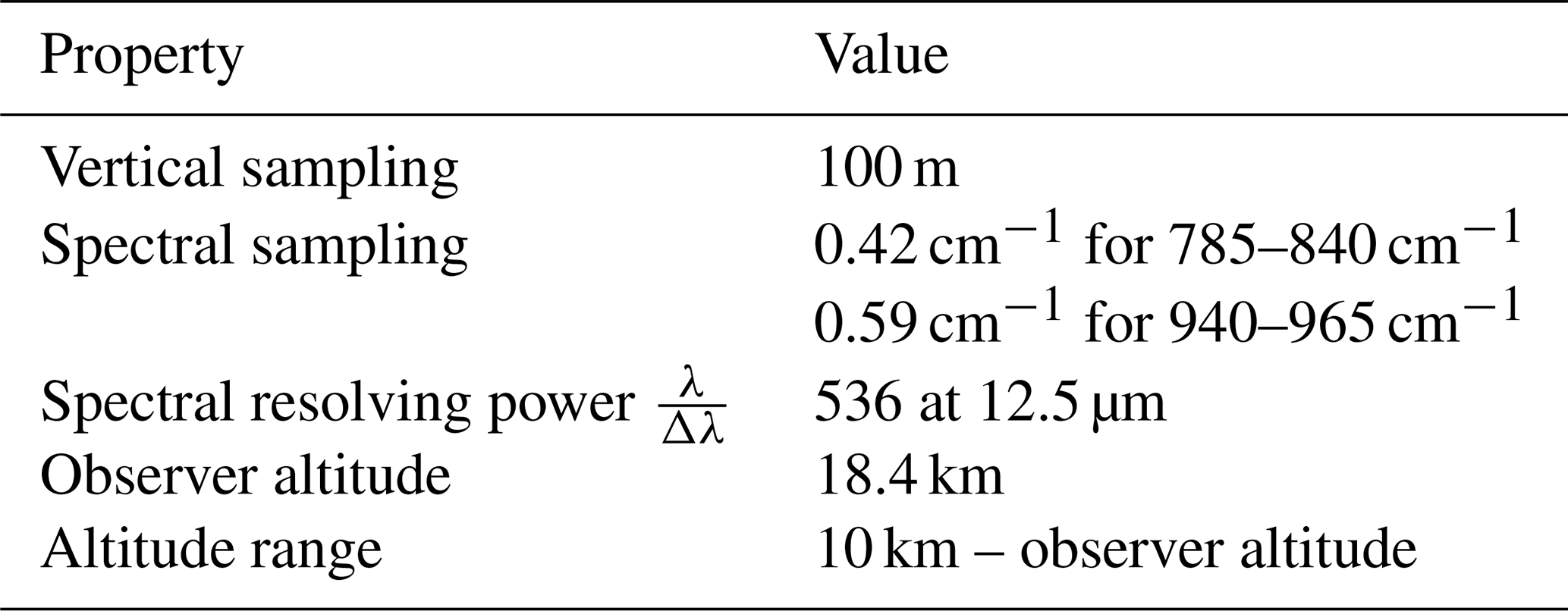
The two important spectral regions that are necessary to analyse infrared spectra with respect to polar stratospheric clouds are 785–840 cm⁻¹, because of the cloud index (CI) and the NAT signature, and the 940–965 cm⁻¹ region, because of an ice signature. The spectral resolving power used in the simulations is $\frac{\mathit{\lambda }}{\mathrm{\Delta }\mathit{\lambda }}$ = 536 at a reference wavelength of 12.5 µm (800 cm⁻¹) (see Weigel, 2009). The spectral sampling of the CRISTA-NF measurements is about 0.0065 µm and corresponds to an average of 0.42 cm⁻¹ for the 785–840 cm⁻¹ wavelength range and 0.59 cm⁻¹ for the 940–965 cm⁻¹ region. These values have been considered in the calculation of the lookup tables for JURASSIC. We used an observer altitude of 18.4 km, which is the maximum average flight altitude during the RECONCILE flights of interest. However, the average altitudes of all flights only differ by a few hundred metres (18.1 to 18.4 km). The observations were simulated in the tangent altitude range from observer altitude down to 10 km. The vertical sampling used for the simulations was 100 m. Table 1 summarises these properties.

Table 1 CRISTA-NF instrument properties used in the simulations.

2.3.2 Atmospheric set-up

For the background atmosphere we used polar winter conditions to get representative simulations. Most information was taken from the MIPAS reference polar winter climatology by Remedios et al. (2007). We updated some constituents, and we focused on the winter 2009–2010 here, especially on January 2010. There are two reasons for this choice: (1) a large variety of PSCs were observed in the Arctic in this winter; and (2) the CRISTA-NF observations of PSCs during RECONCILE took place in January 2010. The updates are summarised in the following.

Two very important parameters of the atmosphere for the simulation of infrared spectra are temperature and CO₂ volume mixing ratios (VMRs). In order to have a temperature profile that is representative for a situation where many different PSCs can occur, we focused on the PSC observation period during the RECONCILE aircraft campaign (17 to 25 January 2010). The temperature profile was derived using ERA-Interim reanalysis data (Dee et al., 2011). An average profile in the region of the CRISTA-NF observations north of Kiruna (67–78^∘ N, 10–35^∘ E) was used for the background atmosphere. Additionally, we used the corresponding pressure profile from ERA-Interim reanalysis data. The CO₂ VMR was derived from the reconstructed CO₂ product by Diallo et al. (2017) for January 2010. The profile is a zonal average in the latitude region of interest. The profiles were extended to larger altitudes following the slope of the climatology. As PAN (peroxyacetyl nitrate) is not included in the climatology, we took a mean profile derived from CRISTA-NF observations (see Ungermann et al., 2012, for the retrieval description) in the region around Kiruna between the end of January and the beginning of March. Unfortunately, there are no retrieval results for PAN available during the PSC flights. However, the derived profile is in a good agreement with published MIPAS-Envisat observations for October to December 2003 in the corresponding latitudinal region (Glatthor et al., 2007) and also with the average profile in 2007–2008 in the latitudinal band from 60 to 90^∘ (Pope et al., 2016). For CFC-11, CFC-113, HCFC-22, SF₆, and COF₂, we updated the climatological profiles to 2010 values using information on tropospheric values (Bullister, 2011) as well as satellite observations from the Atmospheric Chemistry Experiment Fourier Transform Spectrometer (ACE-FTS) (Boone et al., 2013) and in situ observations carried out by the High Altitude Gas Analyzer (HAGAR) instrument (Riediger et al., 2000; Werner et al., 2010) onboard the M55-Geophysica during RECONCILE.

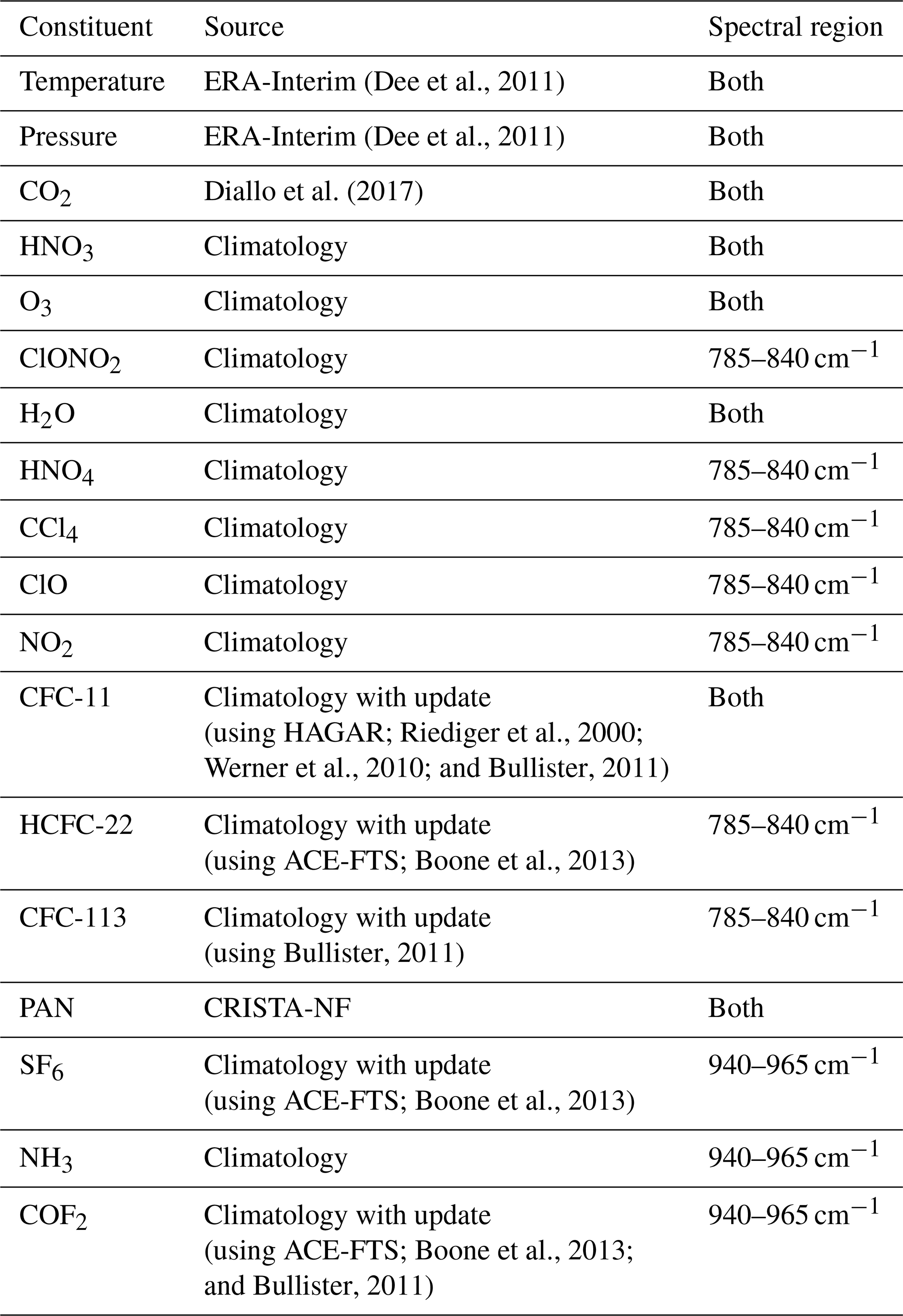
In order to save computation time, we restricted the number of trace gases to a minimum by just using those gases that have a noticeable contribution to the total radiance in the two analysed spectral regions. The trace gases have been selected separately for the two spectral regions. For the 785–840 cm⁻¹ region, we used 13 trace gases: CO₂, HNO₃, ClONO₂, O₃, H₂O, HNO₄, CCl₄, CFC-11, HCFC-22, CFC-113, PAN, ClO, and NO₂. The simulations in the 940–965 cm⁻¹ region included nine trace gases: CO₂, HNO₃, O₃, H₂O, CFC-11, PAN, SF₆, NH₃, and COF₂. A summary of the trace gases, their sources, and the spectral region in which they were considered is given in Table 2.

(Dee et al., 2011)(Dee et al., 2011)Diallo et al. (2017)Riediger et al., 2000Werner et al., 2010Bullister, 2011Boone et al., 2013Bullister, 2011Boone et al., 2013Boone et al., 2013Bullister, 2011

Table 2 Set-up of the background atmosphere for the simulations.

2.4 Cloud scenarios

Two parameters that were largely varied to investigate different situations are the position and the thickness of the PSCs. The PSC position was varied between a minimum cloud bottom height (CBH) of 13 km and a maximum top height of 30 km. For the thickness, we used the values 0.5, 1.0, 2.0, 4.0, and 8.0 km. The bottom height is shifted in 1 km steps up to 20 km (slightly above flight altitude) and in 2 km steps above for each thickness value as long as the cloud top height (CTH) is lower than or equal to 30 km.

PSCs consisting of NAT particles are the most interesting ones for this study due to their impact on the NO_y redistribution. Thus, the majority of the simulations were performed for this particle type. The two parameters varied for the NAT scenarios are the median radius of the particle size distribution and the number density of the particles. The different particle size distributions for all cases (also ice, STS) were described by a log-normal distribution:

$$\begin{array}{}\text{(1)}& {\displaystyle \frac{\mathrm{d}N}{\mathrm{d}r}}={\displaystyle \frac{N_{\mathrm{0}}}{\sqrt{\mathrm{2}\mathit{\pi }}\ln \left(\mathit{\sigma }\right)r}}{e}^{-\frac{\left(\ln \right(r)-\ln (\mathit{\mu }){)}^{\mathrm{2}}}{\mathrm{2}{\ln }^{\mathrm{2}}\left(\mathit{\sigma }\right)}},\end{array}$$

where r is the radius, N₀ is the number density, μ is the median radius, and σ is the width. The width is constant at σ=1.35, and we varied the median radius between 0.5 and 8.0 µm. For the calculation of the number densities and, thus, the particle size distributions, we used different HNO₃ VMRs from 1 to 15 ppbv under the assumption that one HNO₃ molecule is converted to one NAT molecule. The calculations were done for typical conditions for the lower stratosphere with 193 K and 60 hPa.

We also simulated PSCs using bimodal NAT particle distributions. The median radius of the first mode varied from 0.5 to 2.5 µm and was combined with a second mode, where larger radii than in the first mode were used. The total HNO₃ VMR was always 10 ppbv, and the ratios between first and second mode were $\mathrm{70}/\mathrm{30}$, $\mathrm{50}/\mathrm{50}$, and $\mathrm{30}/\mathrm{70}$. Here, we restricted the simulations to two bottom altitudes at 13 and 17 km and three different thicknesses of 1, 4, and 8 km.

The volume densities used for the STS and ice simulations range from 0.1 to 10.0 µm³ cm⁻³ and from 0.1 to 100.0 µm³ cm⁻³ respectively. The median radii were varied between 0.1 and 1.0 µm for STS and between 1.0 and 10.0 µm for ice. In the case of STS, we simulated three different mixtures of H₂SO₄/HNO₃: $\mathrm{2}/\mathrm{48}$, $\mathrm{25}/\mathrm{25}$ and $\mathrm{48}/\mathrm{2}$ wt %.

Finally, we simulated mixed NAT–STS clouds. Here, we also used only the bottom altitudes at 13 and 17 km and the different thicknesses of 1, 4, and 8 km, as in the case of bimodal NAT. Furthermore, we concentrated on the small and medium-sized NAT particles up to 3.5 µm and used three different HNO₃ VMRs of 5, 10, and 15 ppbv. We combined these NAT scenarios with STS scenarios using $\mathrm{2}/\mathrm{48}$ wt %, volume densities of 5 and 10 µm³ cm⁻³, and radii of 0.1, 0.3, and 1.0 µm.

Table 3 Cloud scenario simulation set-up. Please note that “^∗” refers to HNO₃ VMR (ppbv), and “${}^{\ast \ast }$” refers to volume density (µm³ cm⁻³).

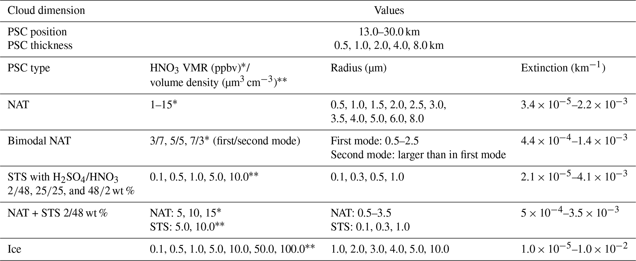
The parameter ranges for all cloud scenarios are summarised in Table 3, including the cloud extinction range. The refractive indices for ice, NAT, and the STS mixtures were taken from Toon et al. (1994), Biermann (1998) with refinement in Höpfner et al. (2006), and Biermann et al. (2000) respectively. The total number of scenarios was 16392 (NAT: 9240; STS: 3360; ice: 2352; and mixtures of bimodal NAT and NAT–STS: 1440).

Considering the computational resources required to simulate this number of scenarios, we assumed single scattering. Neglecting multiple scattering introduces uncertainties. Based on the findings of Höpfner and Emde (2005) for our optical depth ranges (Table 3, extinction times cloud thickness) and the single-scattering albedos of STS, NAT, and ice, the uncertainty is mostly below 1 %, 4 %, and 4 % respectively. However, for a few scenarios of 8 km thickness, the uncertainty may reach up to 4.5 % for STS and 20 % for ice. In the cloud scenario set-up, we assumed homogeneous clouds. The horizontal extent of the CRISTA-NF line of sight inside the PSC can reach up to several hundred kilometres. In the case of synoptic-scale PSCs, horizontal homogeneity is a sufficiently good approximation. PSCs of other origin, such as mountain-wave-induced PSCs, have a smaller horizontal extent but are less frequent compared with synoptic-scale PSCs.

3 Results of the simulations

The following section deals with the analyses of the simulation results. The analyses can be divided into three parts: (1) the shift in the NAT feature, (2) the detection of PSCs and the identification of the NAT and ice PSC types, and (3) the determination of the bottom altitude of the clouds.

3.1 Shift in the NAT feature

The appearance of the spectral feature that is observed in infrared limb spectra in the presence of polar stratospheric clouds consisting of NAT particles in our study is unambiguously characterised by the median radius of the particle size distribution, as we kept the distribution width σ constant. With increasing median radius, the shape transforms from the well-known pronounced peak at about 820 cm⁻¹ to a peak that is slightly shifted towards smaller wavenumbers and, finally, to a step-like feature. Figure 1 illustrates this behaviour and the dependency of the appearance on the median radius. The spectra shown in Fig. 1 are scaled such that the radiance in the 832.0–834.0 cm⁻¹ spectral range is equal to one for all spectra. The example spectrum for the smallest median radius of 0.5 µm (yellow colour) exhibits a clear pronounced peak at about 820 cm⁻¹. For slightly larger median radii (1.0–3.5 µm), the peak shifts to smaller wavenumbers and becomes less pronounced (orange colours). When the median radius is even larger, the spectral feature transforms to a step-like feature that shows a steep radiance decrease from about 811 to 826 cm⁻¹. The magnitude of this decrease largely diminishes with increasing median radius.

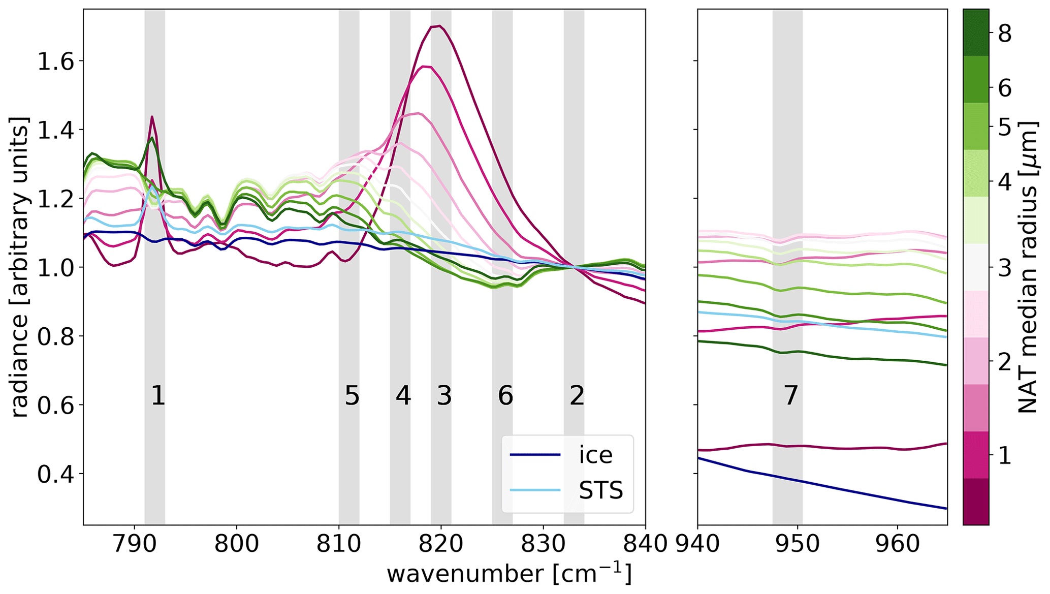
Figure 1 Selected simulation results for infrared spectra in the presence of polar stratospheric clouds consisting of NAT particles with different particle median radii, STS, and ice. The spectra have been scaled using the mean radiance in the 832.0–834.0 cm⁻¹ (MW2) spectral window such that the radiance for all spectra equals one in this window. The grey vertical bars mark the micro-windows (MWs) used during the analysis; they are numbered from MW1 to MW7.

This behaviour and, thus, the dependency of the appearance of the feature on the median radius can be explained by the different contributions of emission and scattering to the total observed radiance enhancement caused by the PSCs. These contributions largely depend on the median radius of the particles. The real and the imaginary part of the refractive index of β-NAT are shown in Fig. 2a in black and red respectively. The imaginary part illustrates the emission and absorption characteristic of the NAT particles, whereas the real part shows the scattering behaviour. The imaginary part shows a distinct peak at about 820 cm⁻¹. As the emission is the major contribution when only small particles are present, the simulated spectra in the case of small NAT only show this peak. This is illustrated in Fig. 2b and c, where the extinction and single-scattering albedo (SSA) are shown. The extinction shows a clear peak at about 820 cm⁻¹, and the SSA, which gives the contribution of the scattering to the total extinction, shows low values. With increasing median radius of the NAT particles, the scattering becomes more and more important. This can be seen by the increase in the SSA, which for large particles then can exceed 0.5, i.e. the scattering increasingly accounts for more than half of the total extinction. As a consequence, the peak shifts to smaller wavenumbers with increasing particle size until it transforms to a step-like signature (see Figs. 1 and 2b).

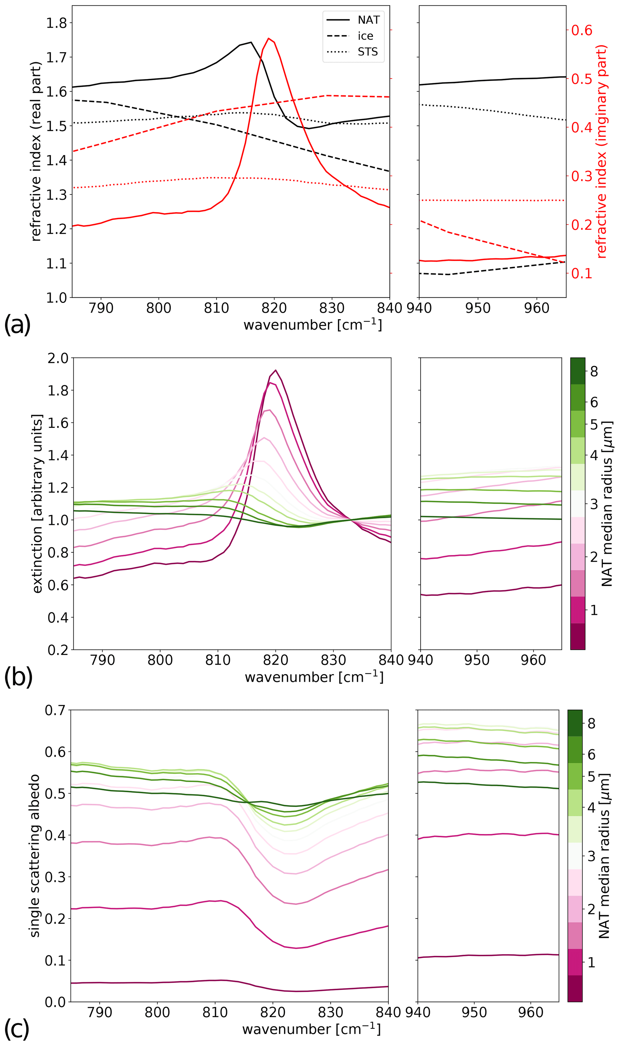
Figure 2 (a) Refractive indices for NAT (solid lines), STS (dotted lines), and ice (dashed lines). The real parts are shown in black, and the imaginary parts are shown in red using the right y axis. The refractive indices for NAT, STS, and ice were taken from Biermann (1998) with refinement in Höpfner et al. (2006), Biermann et al. (2000), and Toon et al. (1994) respectively. (b) Extinction spectra for NAT with different median radii. The spectra have been scaled using the mean value in the 832.0–834.0 cm⁻¹ spectral window such that the extinction for all spectra equals one in this window. (c) Single-scattering albedo for NAT with different median radii.

The spectral feature with all its versions in the 810–820 cm⁻¹ region is a unique signature that only occurs in the presence of NAT PSCs and will be used for the detection of NAT PSCs. Other PSCs consisting of STS or ice do not show this feature, as shown in Fig. 1 using two examples in light blue (STS) and dark blue (ice). In contrast to the other PSC types, ice shows the largest relative difference between the 832.0–834.0 cm⁻¹ region and the second spectral range of our simulations (940–965 cm⁻¹). Only NAT PSCs consisting of particles with very small radii (< 1.0 µm) can also achieve large differences. This spectral behaviour in the case of ice will further be used to detect ice PSCs.

3.2 Detection of NAT

3.2.1 Unimodal pure NAT

The detection of clouds using infrared limb spectra typically uses the cloud index (CI) (e.g Spang et al., 2001, 2002, 2008). The CI is the radiance ratio between a spectral region dominated by CO₂ at around 792 cm⁻¹ and a second spectral region dominated by aerosol or cloud particles at around 833 cm⁻¹. For the analysis of the airborne observations by CRISTA-NF, we used the 791.0–793.0 cm⁻¹ (micro-window MW1) and 832.0–834.0 cm⁻¹ (MW2) windows. Because of the different viewing geometries and instrument properties, the first window is defined with a smaller range than that typically used for satellite observations (Spang et al., 2008). In cloud-free conditions, the CI value (MW1/MW2) is typically large (around 10). When clouds or larger aerosol loads are in the line of sight of the instrument, the CI significantly drops to smaller values depending on the optical thickness of the cloud. The MWs used for the CI and all following indices are marked with grey bars in Fig. 1. Additionally, all indices are summarised in Table 4.

Table 4 Summary of the indices and their corresponding micro-windows.

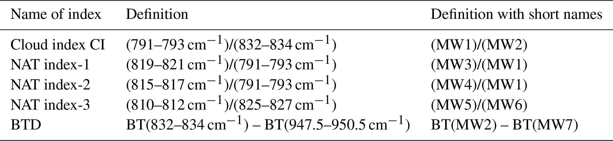
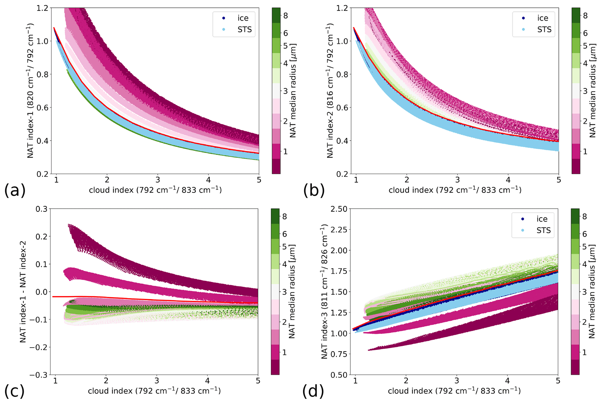
Figure 3 Correlations between different NAT indices and the cloud index for the simulated PSC scenarios: (a) NAT index-1 (819–821 cm⁻¹)/(791–793 cm⁻¹); (b) NAT index-2 (815–817 cm⁻¹)/(791–793 cm⁻¹); (c) NAT index-1 – NAT index-2; (d) NAT index-3 (810–812 cm⁻¹)/(825–827 cm⁻¹). The red lines show the separation lines, which mark the upper envelope of the regions of STS and ice defined by the blue coloured areas (in panels a, b, and d) and the region of medium and large NAT with radii greater than 1.0 µm (in panel c). Simulation results for ice and STS are in shown in dark and light blue respectively.

The detection of NAT particles inside clouds is based on the characteristic spectral behaviour in the 810–820 cm⁻¹ region. In previous studies, a NAT index, the radiance ratio between the spectral region of the typical NAT feature (819–821 cm⁻¹) and the region of the CO₂ peak (788–796 cm⁻¹), was introduced to detect PSCs containing small NAT particles (e.g Spang and Remedios, 2003; Höpfner et al., 2006; Spang et al., 2012, 2016, 2018). Here, we define the NAT index-1 as the radiance ratio between the 819–821 cm⁻¹ (MW3) and 791–793 cm⁻¹ (MW1) regions and use the same smaller window in the region of the CO₂ peak as for the CI. In a scatter plot of the NAT index-1 versus the CI, we found that spectra simulated for small NAT particles were separate from spectra simulated for larger NAT particles and other types of PSCs (Fig. 3a). Note here that there is sometimes an overlap of the data points for adjacent radii. This is also the case in the other scatter plots. Nearly all simulations with NAT particles < 3 µm lie above the region of the simulations for STS and ice clouds, which is marked by the solid red line. The separation line was determined solely by the simulation results for ice and STS to define an upper limit of these simulations for each possible CI value. Thus, NAT particles within this size range can be detected and discriminated using NAT index-1.

In order to detect PSCs containing larger NAT particles and to make the estimation of the size range of the particles more distinct, we introduce two new NAT indices here. The NAT index-2, which is defined as the radiance ratio between 815–817 cm⁻¹ (MW4) and 791–793 cm⁻¹ (MW1), focuses on the shifted NAT feature that occurs for larger particles than that producing the non-shifted feature. Figure 3b shows the scatter plot of the NAT index-2 versus the CI. In contrast to the NAT index-1, the results for PSCs with larger NAT particles (up to 4 µm) now also lie above the simulations for STS and ice (red separation line). Additionally, for different particle median radii, the distance to the separation line changes when going from NAT index-1 to index-2 in an inverse way. In the case of very small particles, the distance becomes smaller as the spectral region used for the detection moves away from the centre of the typical NAT peak. For larger particles, the opposite behaviour is observed, and the distance enlarges as the spectral region moves to the centre of the shifted NAT peak. This inverse behaviour can be seen in Fig. 3c, where the difference between NAT index-1 and index-2 is shown on the y axis. It is obvious that the simulations for the two smallest radii (0.5 and 1.0 µm) behave in an inverse manner to the simulations for larger radii.

Lastly, we introduce the NAT index-3, which is defined as the radiance ratio between 810–812 cm⁻¹ (MW5) and 825–827 cm⁻¹ (MW6), to detect PSCs containing even larger NAT particles. This ratio enables the discrimination of a step-like feature from a peak and a more or less constant radiance in the complete spectral range as is the case for STS and ice. Figure 3d shows the scatter plot of the NAT index-3 against the CI. The simulation results for small NAT particles (≤ 1.0 µm) have a NAT index-3 smaller than for the simulations results for STS and ice. A large part of the simulation results for larger NAT particles show a NAT index-3 that is larger than for the simulation results for STS and ice. By using this ratio NAT particles with radii > 4 µm also separate from the other simulation results and are consequently detectable.

Figure 4 The histograms of the proportion of the detected spectra (NAT) per simulated cloud spectra in each size bin. The colours illustrate the different cases (1–3): case 1 (sNAT) is shown in yellow, case 2 (mNAT) is shown in orange, and case 3 (lNAT) is shown in red. For a description of the different cases, see the text. In panel (a), the CI threshold value to detect a spectrum as a cloud spectrum is 5.0 (about 365 000 cloud spectra in total), whereas the threshold in panel (b) is 3.0 (about 197 000 cloud spectra in total).

In total, the three different NAT indices enable the detection of PSCs containing NAT particles and allow for a classification of the NAT particles in different size regimes. The detection and discrimination of NAT can be divided into three different cases: case 1 (small NAT) – NAT is detected using the NAT index-1, and the difference NAT index-1 – index-2 is above the separation line; case 2 (medium NAT) – NAT is detected using the NAT index-2, and the difference NAT index-1 – index-2 is below the separation line; and case 3 (large NAT) – no detection of NAT using the NAT index-1 or index-2 (both below separation line), but the NAT index-3 is above the separation line. Figure 4 shows the proportion between the spectra detected as being influence by NAT and the cloud spectra (spectra below a certain CI threshold) in each size bin of the simulations (0.5–8.0 µm), colour coded for the three different cases. In Fig. 4a, only observations with a CI below 5.0 are taken into account. Obviously, in case 1 (yellow colour), only NAT particles with a median radius of 0.5 or 1.0 µm are detected. The detection results in case 2 (orange colour) go from 1.5 up to 4.0 µm, and the results in case 3 (yellow colour) all show median radii larger than or equal to 2.5 µm, whereby the radius 2.5 µm only occurs in a very small amount. Thus, the different cases all represent a specific size regime with little or no overlap with the other cases. Particularly the very small NAT particles (0.5 and 1.0 µm) can be completely distinguished from the particles with other median radii, as all of the detected spectra in this size range fall into case 1. The other two cases overlap with each other.

The total detection capacity with respect to the simulations is also very good. For median radii up to 6.0 µm, nearly all spectra that have been detected as cloud spectra can be detected as spectra influenced by NAT particles. However, a few cloud spectra cannot be identified as NAT spectra for 2.5 and 3.0 µm. These spectra all have a larger CI value (> 3.0, optically thinner), and the separation between NAT and the other PSC types degrades for larger CI values (see Fig. 3). Thus, a small part of the cloud spectra influenced by NAT cannot be distinguished from STS and ice. When the CI threshold value is reduced to 3.0, the detection itself and also the separation between the different size regimes improves, as shown in Fig. 4b. Now all spectra for median radii up to 6.0 µm are identified as NAT. Additionally the separation between the different sizes is now better, and case 3 only detects radii ≥ 3.5 µm. Independent of the CI threshold value, only a part of the simulations for the largest median radius of 8.0 µm are detected as NAT (CI < 5.0: ∼ 30 %; CI < 3.0: ∼ 40 %). This is caused by the decreasing magnitude of the radiance decrease from 811 to 826 cm⁻¹ for an increasing median radius (see Sect. 3.1). The improvement in the detection and discrimination when using a CI threshold of 3.0 shows that it is not advisable to use a larger threshold when analysing observations. According to the different size ranges of the three cases, the cases are hereafter denoted as small NAT (sNAT: ≤ 1.0 µm), medium NAT (mNAT: 1.5–4.0 µm), and large NAT (lNAT: ≥ 3.5 µm). Compared with the former method where only the NAT index-1 is used (e.g. Spang and Remedios, 2003; Höpfner et al., 2006; Spang et al., 2012, 2016, 2018), our new approach with three NAT indices enables an improved detection capacity, as more NAT clouds can be detected. For our simulations, the improvement is about a factor of 1.78 (approximately 190 000 cloud spectra identified as NAT with all new indices and about 108 000 spectra identified as NAT when only using index-1) for a CI < 3.0.

3.2.2 Influence of tropospheric clouds

The influence of tropospheric clouds was intensively studied during the analysis of the radiative transfer simulations for various PSC situations for the MIPAS-Env satellite instrument (Spang et al., 2012, 2016), and the results can be transferred to this study. A tropospheric cloud below the PSC mainly influences the absolute radiance values where the cold tropospheric cloud leads to lower overall radiance values. The appearance of the spectral signature (typical peak, shifted peak, or step-like behaviour) in the 810 to 820 cm⁻¹ region remains nearly unchanged. Simulations by Woiwode et al. (2019) also showed these effects. As our detection method is based on colour ratios, i.e. relative effects, the change in the absolute radiance values does not significantly influence the analysis. Especially in the case of STS or ice, which show no distinct spectral features in the 810–820 cm⁻¹ region, the data points in the scatter plots only slightly shift along the correlation lines or regions for the specific PSC type. Thus, the separation lines, which are defined using the STS and ice simulations (see Fig. 3), are still valid in such cases. Consequently, a false detection by an assignment of STS or ice to a NAT class is not possible. For NAT clouds, the impact of underlying clouds slightly depends on the median radius of the particles, as the scattering contribution increases with radius (see Fig. 2c). For median radii ≤ 1.0 µm, an influence of a tropospheric cloud is negligible, as the spectra are dominated by absorption and emission. For larger median radii a little change in the features can occur and a little change in the positions of the data points in the scatter plots is possible. Possible effects are an eventual assignment of NAT with a median radius of 1.5 µm to the class sNAT (upward shift in data points for the difference NAT index-1 – NAT index-2) or a missing detection for lNAT (downward shift in data points for NAT index-3). Thus, a very small part of the uncertainty in the class boundaries cannot be completely ruled out. However, the majority of all possible situations will still be detected and classified correctly.

3.2.3 Mixed NAT–STS clouds

We additionally simulated mixed NAT–STS clouds to evaluate the influence on the spectra and, specifically, the performance of our classification into different size regimes. Here, we only simulated a subset of all possible combinations, as the spectral behaviour for each median radius is very similar independent of factors such as the bottom altitude of the cloud or the thickness (see Sect. 2.4).

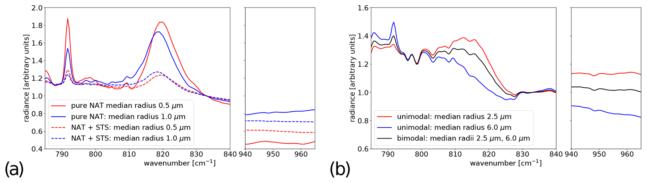
Figure 5 Selected spectra for NAT–STS mixed clouds (a) and bimodal NAT particle size distributions (b). The spectra were scaled using the mean radiance in the 832.0–834.0 cm⁻¹ spectral window such that the radiance for all spectra equals one in this window. (a) The solid lines show spectra for unimodal NAT particle size distributions. Red denotes a median radius of 0.5 µm and 10 ppbv HNO₃, and blue denotes a median radius of 1.0 µm and 10 ppbv HNO₃. The dashed lines show the NAT–STS mixed clouds. The amount of NAT is the same as for the pure NAT simulations, and the volume density of STS is 10 µm³ cm⁻³ in both cases. (b) The red and blue lines show the spectra for unimodal size distributions with median radii of 2.5 and 6.0 µm respectively. The amount of HNO₃ is 10 ppbv in each case. The black line shows the simulation results for a bimodal size distribution with median radii of 2.5 and 6.0 µm and 5 ppbv HNO₃ in each mode.

If STS is present in addition to NAT, the relative magnitudes of the spectral features caused by NAT particles get smaller; therefore, the separation between these mixed clouds and STS is also restricted compared with a pure NAT cloud. Figure 5a shows example spectra for PSCs of pure NAT (solid lines in red for 0.5 µm and blue for 1.0 µm) and PSCs with the same NAT as well as STS (dashed lines) to illustrate this effect. In a scatter plot of the NAT indices versus the CI (compare Fig. 3a and b), the simulation results for the NAT–STS mixtures are closer to the separation line or even below it compared with pure NAT. When the NAT detection and classification procedure (described in the previous subsection) is applied to the simulation results for the mixed clouds, the good discrimination between the small and medium-sized particles remains. This discrimination relies on the difference in the NAT index-1 and index-2, where both indices are influenced in the same way. Therefore, the sign of the difference remains the same, because it depends on the position of the spectral peak, which is not affected by the additional STS (see Fig. 5a). For a CI value below 3.0, about 97.5 % of the simulated cloud spectra with median radii of 0.5 and 1.0 µm are correctly detected as sNAT, and only about 0.3 % are incorrectly detected as mNAT (the remaining 2.2 % are not detected as NAT). In some cases STS completely masks the spectral features caused by NAT, and NAT is not detectable any more. However, for a CI value below 3.0, more than 90 % of the cloud spectra can still be identified as containing NAT in the entire simulated size range. The proportion typically decreases with increasing median radius, i.e. more NAT-influenced spectra at 3.0 µm are missed than at 0.5 µm, and will also decrease with increasing STS volume density or decreasing HNO₃ VMR inside the PSC. In a nutshell, in mixed NAT–STS clouds, fewer scenarios are identified as containing NAT, because the STS reduces the amplitude of the characteristic NAT signature. However, if a scenario in our simulations was classified as NAT, the size attribution remains as reliable as in the pure NAT scenarios.

3.2.4 Bimodal NAT clouds

In addition, we also simulated PSCs using bimodal NAT particle distributions with a main focus on the small and medium-sized particles and the separation between those. Here, a subset of all possible combinations was also simulated (see Sect. 2.4).

The spectra simulated for the bimodal NAT particle size distributions are typically some kind of mixture of the spectra for the corresponding unimodal distributions; thus, the HNO₃ VMR ratio plays an important role. Figure 5b shows an example of a spectrum simulated for a bimodal NAT particle distribution (black line). The HNO₃ VMRs were 5 ppbv in each mode with median radii of 2.5 and 6.0 µm. The two corresponding spectra for the unimodal size distributions are shown in red and blue respectively. Obviously, the spectrum for the bimodal size distribution is a mixture of the other two. When the HNO₃ ratio for both modes is changed to $\mathrm{70}/\mathrm{30}$ or $\mathrm{30}/\mathrm{70}$, the spectrum looks more like the spectrum for the unimodal size distribution that dominates the bimodal distribution, because of more HNO₃ in the corresponding size range.

We also applied our classification procedure to these simulations for bimodal size distributions with the following results. When the first mode dominates (70 % HNO₃), nearly all cloud spectra simulated for a median radius of 0.5 or 1.0 µm are still detected as sNAT (about 99 % sNAT and 1 % mNAT) and, thus, classified correctly. All spectra that are identified as cloud (CI < 3.0) are also identified as NAT-containing PSCs. For a HNO₃ ratio of $\mathrm{50}/\mathrm{50}$ or $\mathrm{30}/\mathrm{70}$, the influence of the second mode increases such that more and more spectra are detected as mNAT and a small part are detected as lNAT. In the case of a $\mathrm{50}/\mathrm{50}$ ratio, about 50.5 % are classified as sNAT and 49.5 % are classified as mNAT; for a $\mathrm{30}/\mathrm{70}$ ratio, 21 % are classified as sNAT, 77 % are classified as mNAT, and 2 % are classified as lNAT. When combined with larger NAT particles in the second mode (≥ 4 µm), a part of the cloud spectra (CI < 3.0) are not detected as NAT because neither a spectral peak nor a step-like behaviour can be detected ($\mathrm{50}/\mathrm{50}$: 0.5 % and $\mathrm{30}/\mathrm{70}$: 10 %). However, these cases are only a few percent of all cloud spectra in our simulations. When the first mode has a median radius between 1.5 and 2.5 µm, about 99 % of the simulated spectra are identified as mNAT (1 % lNAT, when the median radius in the second mode is 5.0 or 6.0 µm) independent of the ratio of the HNO₃ VMRs. Furthermore, only a few spectra per thousand of those identified as clouds cannot be classified as NAT-containing PSCs. In total, our new classification scheme delivers very reasonable results even in the case of bimodal NAT particle size distributions.

3.3 Detection of ice

The detection of ice uses the fact that a large radiance decrease from about 833 to 949 cm⁻¹ can be observed in the presence of ice (see Fig. 1). This clear decrease is only observed in the case of ice or in the presence of very small NAT particles. Spang et al. (2012, 2016) used this spectral behaviour to detect ice clouds in satellite measurements of MIPAS-Envisat. The authors used the brightness temperature (BT) difference between the two spectral regions. Here, we adopt the same method for the CRISTA-NF observations. Because of the different viewing geometry, spectral resolution, and the different definition of the CI for the two instruments, the separation lines have to be newly defined. The spectral regions used for the BT difference are 832.0–834.0 cm⁻¹ (MW2) and 947.5–950.5 cm⁻¹ (MW7). In a scatter plot of the BT difference against the CI, the simulated ice spectra clearly separate from other particle types (Fig. 6). Obviously, spectra that are influenced by ice clearly separate from STS and nearly all NAT particles when the cloud is optically thick enough (low CI). For larger CI, values the separation becomes smaller. The only particles that can produce similar values of the BT difference are very small NAT particles with median radii of 0.5 µm (yellow colours in Fig. 6a), but these particles can be safely filtered out using the method described in Sect. 3.2. Consequently, the BT difference is a very robust method to detect ice particles in PSCs.

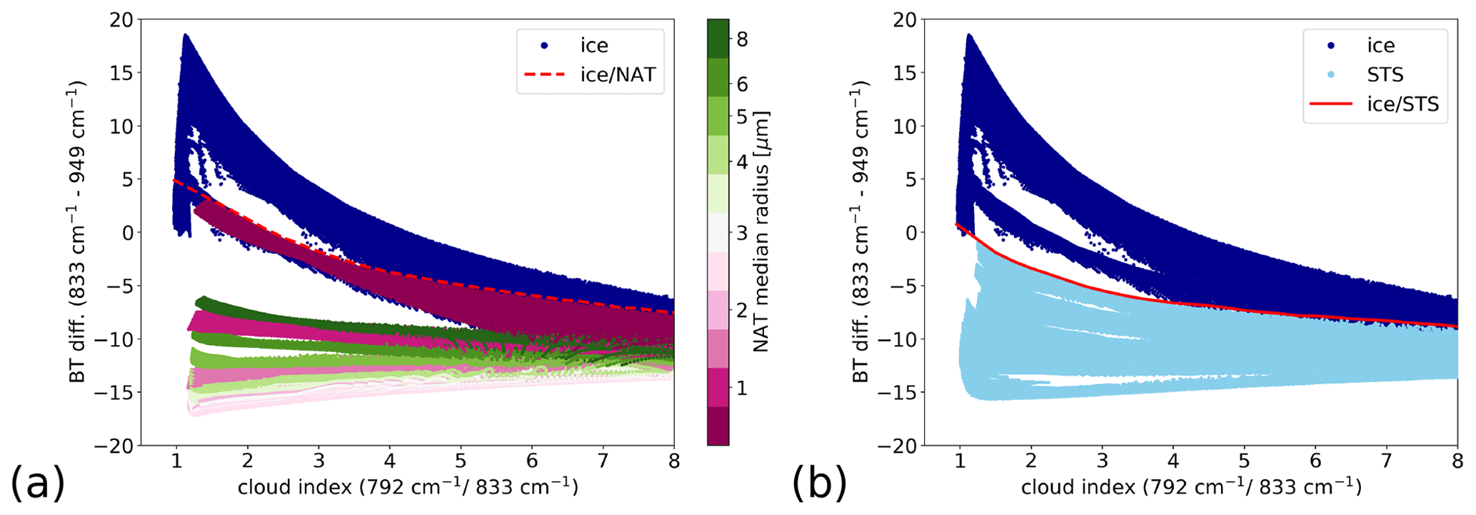
Figure 6 Correlation between the BT difference (832–834 cm⁻¹) – (947.5–950.5 cm⁻¹) and the cloud index. The red solid line shows the separation line between ice and STS, and the dashed line marks the separation between ice and NAT.

3.4 Detection of STS

The spectra for STS show neither a local spectral feature like the spectra for NAT nor a broadband spectral feature such as the spectra for ice. Thus, the detection of STS can not be achieved by using a unique spectral behaviour. In practice, the detection procedure is as follows. Firstly, the NAT detection methods are used to detect observations of NAT particles and to distinguish between the three size regimes. Secondly, the BT difference method is applied to the observations to detect ice. Finally, the observations inside PSCs that are neither detected as NAT nor as ice are categorised as STS. It is not necessarily the case that the spectra categorised as STS are solely influenced by STS; it is possible that NAT or ice were also present in the PSC, but the additional amount of STS was enough to minimise the spectral features such that NAT or ice was no longer definitely detectable. Furthermore, the small amount of very large NAT particles that cannot be distinguished from STS and ice will also fall into the STS category.

3.5 Bottom altitude of the PSCs

Further important quantities with respect to cloud detection are the vertical thickness and the position of the cloud defined by the top and bottom altitude. Here, we present a method to determine the bottom altitude of the observed cloud. The cloud index, which is used to detect optically thick conditions caused by clouds (or aerosol), shows characteristic vertical changes in the presence of clouds. These changes are used for the detection of the cloud bottom altitude.

Figure 7 Vertical profiles of the cloud index (a) and the vertical gradient of the cloud index (b) for clouds with different vertical thicknesses. The colour coding shows the vertical thickness (yellow: 1 km; red: 4 km; light blue: from 8 to 23 km). The HNO₃ VMRs inside the NAT PSCs are 5 ppbv for the 1 and 8 km thick clouds and 10 ppbv for the 4 km thick cloud. The corresponding shaded areas illustrate the vertical extent of the clouds. The black stars mark the altitudes of the CI minima and the CI gradient minima. The black horizontal line shows the flight altitude.

Figure 7a shows examples of CI altitude profiles for clouds with different vertical thicknesses. When the complete cloud is located below the flight altitude (yellow colour), the CI largely drops to low values when entering the cloud from above (or slightly above because of the FOV). In the case that the flight altitude is inside the cloud, the CI is already low at flight altitude. The CI then typically further decreases with decreasing altitude inside the cloud, and the minimum CI value is reached close to the bottom altitude. In some cases, when the vertical thickness is larger (4 km or 8 km), the CI minimum can be located somewhere inside the cloud. When leaving the cloud, the CI increases again. These vertical changes in the CI can be best illustrated with the gradient of the CI (Fig. 7b). Slightly above the cloud top, the vertical gradient maximises, and slightly below the cloud bottom, the gradient reaches its minimum value. In contrast to the CI minimum, where larger deviations from the cloud bottom can occur, the minimum of the gradient is always slightly below the real bottom altitude of the cloud.

Figure 8 summarises the results for the simulated clouds with a bottom altitude below flight altitude. In the case of the CI minima (full circles), there are sometimes larger deviations from the real bottom altitude when the cloud is vertically thick (red and light blue full circles). The CI gradient minima (full diamonds) are always located close to the real bottom altitude, at the first or the second measurement below. The possibility to observe the gradient minimum at the second measurement below the cloud increases with decreasing altitude of the cloud, because the vertical extent of the FOV (in metres) is larger at lower altitudes. In our simulations, this occurs only at bottom altitudes of 13.0 and 14.0 km. In summary, the CI minimum and the gradient minimum enclose the real bottom altitude. A large gap between the two minimum values indicates the observation of a cloud with a larger vertical thickness.

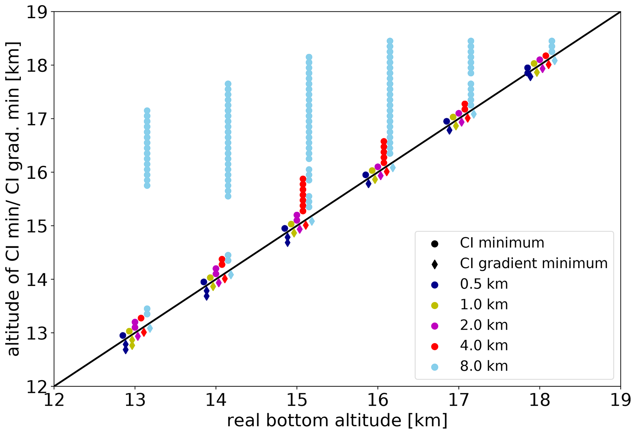
Figure 8 The altitude of the CI minimum (full circles) and the CI gradient minimum (full diamonds) against the real bottom altitude. The black line shows the line with a slope of one. The different cloud thicknesses are shown using colour coding, and the points have been shifted along the line for the sake of clarity. Clouds with a CI minimum < 1.2 (optically thick) and > 5.0 (optically thin) have been excluded.

There are further restrictions on the determination of the bottom altitude. In some cases, the observations run into saturation, and the CI values below the cloud bottom altitude converge at a low value. Additionally, in other situations, the CI values below the bottom altitude only show a linear increase and not the larger change directly below the bottom altitude. In both cases, the CI minimum and the gradient minimum cannot sufficiently be determined and used for the detection of the bottom altitude of the cloud. An effective way to sort out observations that are possibly affected is the use of a threshold value. We derived a CI minimum below 1.25 from the simulations. Such low CI values only occur for a part of the ice clouds simulated here (typically for largest volume densities of 50 and 100 µm³ cm⁻³; with increasing vertical thickness, some simulations with 5 and 10 µm³ cm⁻³ were also affected) and for a few of the NAT and STS clouds with large HNO₃ VMRs (≥ 11 ppbv) or volume densities (≥ 5 µm³ cm⁻³) combined with a large vertical thickness (≥ 4 km). Secondly, when the cloud is optically and vertically thin, the location of the cloud bottom is also not detectable. In order to select only clouds that are optically thick enough for detection, we used only simulation spectra with CI < 5.0.

Furthermore, other special situations can be considered, such as PSC only above flight altitude and layered PSCs. When the PSC is located above the flight altitude, the CI typically increases with decreasing altitude from flight altitude downwards, as the length of the line of sight inside the PSC also decreases. Thus, there is not the typical decrease in the CI to a local minimum, but rather a continuous increase from a rather low CI value compared with clear air at flight altitude. Both the CI and the CI gradient typically show the lowest values at the points closest to the flight altitude. In the case of layered PSCs, where different types of PSCs are lying above each other, the results depend on the optical thickness of the different layers. On the one hand, the CI gradient minimum is still located at the bottom of the complete PSC, when the lower layer is optically thick enough and the transition to the cloud-free atmosphere shows the largest increase in CI; on the other hand, when the lower layer is optically very thin, it can occur that the CI gradient minimum is located directly below the upper layer. In this case, the transition from the upper layer to the lower layer leads to a larger increase in the CI than the transition from the lower layer to the cloud-free atmosphere.

4 Application to the CRISTA-NF measurements

This section shows the application of the methods derived from the simulations to observations from the CRISTA-NF instrument for all flights during RECONCILE where PSCs were observed. These PSC observations were carried out during the first five flights between 17 and 25 January 2010. For one selected flight (local flight 3: 22 January 2010), we additionally show more details of the results to demonstrate the capability of the instrument and the methods.

4.1 Analysis of the CRISTA-NF measurements

We applied the detection methods for NAT and ice using the NAT indices and the brightness temperature difference (BTD) to the measurements from CRISTA-NF for flight 1–5. The results for the different scatter plots are shown in Fig. 9a–e. Note here that the measurements were filtered for flight 2–5 so that only measurements inside PSCs were taken into account (for more details, see Sect. 4.2). In the case of flight 1, this filtering was not possible as many profiles show very low CI values (see Sect. 3.5); thus, all measurements between flight altitude and 14 km are shown for this flight. The observations separate into two different situations. First, during flight 1, a clear ice signal was detected, which can been seen in Fig. 9e, and there was no indication of NAT. For all NAT indices versus CI, the data points stay below the separation lines, which were derived from the simulation results, in the same way as the simulation results for ice (see Fig. 3). This shows the good correspondence between simulations and observations and gives additional confidence in the simulation results and the derived separation lines using these results. The ice observation is supported by European Centre for Medium-Range Weather Forecast (ECMWF) data (not shown), which show temperatures low enough for ice formation above the flight altitude (at about 20 km and above), and CALIPSO observations that show ice PSCs above 20 km a few hours before the flight (Michael Pitts, personal communication, 2020). Thus, CRISTA-NF observed the ice PSC from below. As ice PSCs are typically optical thicker than other PSCs, this explains the lower CI values observed during this flight. Second, flights 2–5 all show NAT signatures (see Fig. 9a and b). As the differences between NAT index-1 and index-2 are below the separation line (see Fig. 9c), these observations are categorised as mNAT (a few spectra are categorised as lNAT for flight 5). The difference in the spectra for these two PSC types is additionally illustrated in Fig. 9f, with example spectra from flight 1 (blue colours) and flight 3 (red colours). They are scaled for better comparability. Obviously, the spectra in flight 3 show a shifted NAT peak, and the spectra in flight 1 show a large negative gradient towards larger wavenumbers, which in the absence of the of the 820 cm⁻¹ NAT feature clearly shows the influence of ice (see Fig. 1).

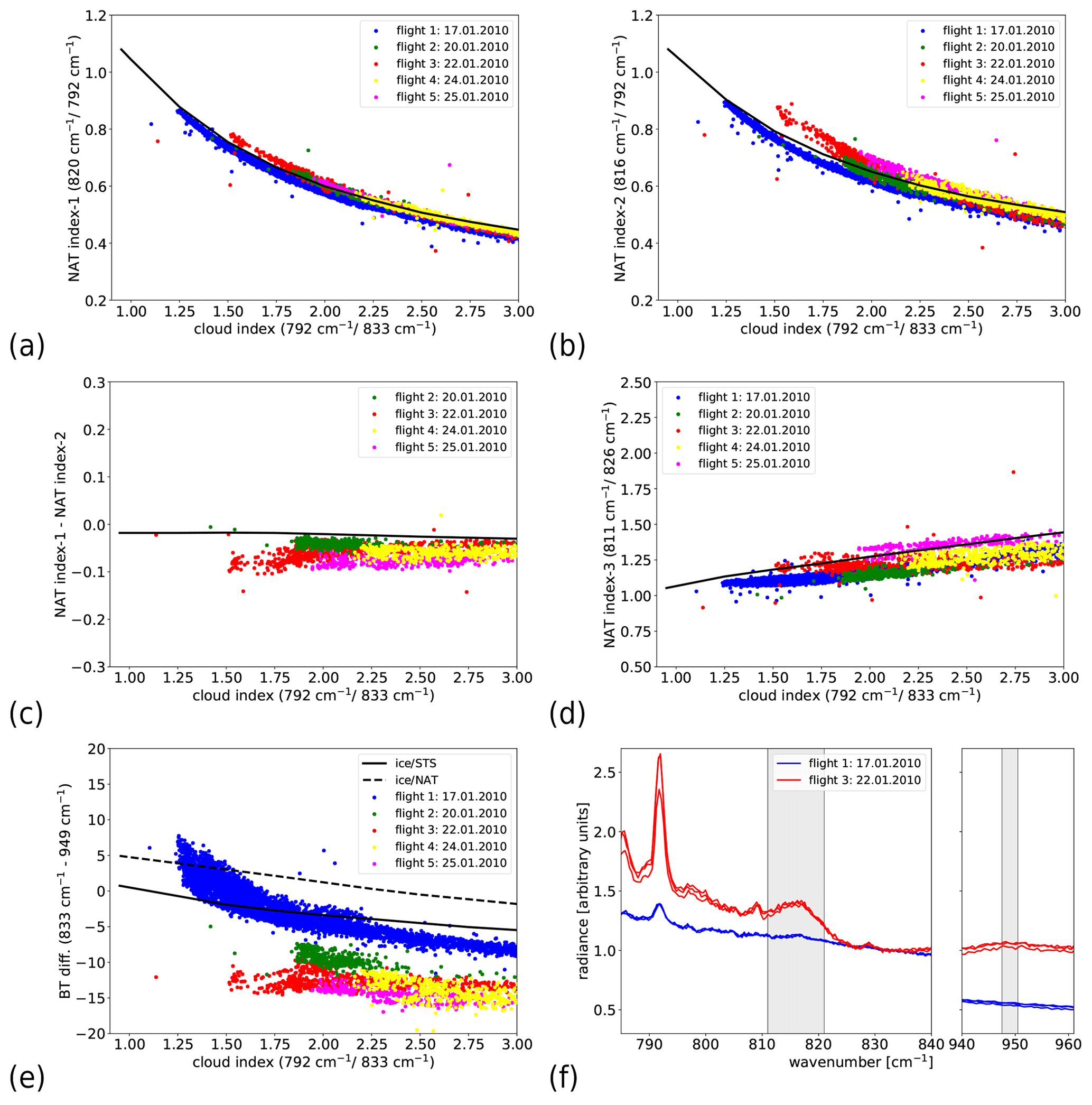
Figure 9 Correlations between the different NAT indices and the cloud index for the CRISTA-NF observations during RECONCILE flights 1–5: (a) NAT index-1 (819–821 cm⁻¹)/(791–793 cm⁻¹) (MW3/MW1); (b) NAT index-2 (815–817 cm⁻¹)/(791–793 cm⁻¹) (MW4/MW1); (c) NAT index-1 – NAT index-2; (d) NAT index-3 (810–812 cm⁻¹)/(825–827 cm⁻¹) (MW5/MW6). The black lines show the separation lines, which mark the upper envelope of the regions of STS and ice (in panels a, b, and d) or the region of medium and large NAT (in panel c). Simulation results for ice and STS are in shown in dark and light blue respectively. (e) Correlation between the BT difference (832–834 cm⁻¹) – (947.5–950.5 cm⁻¹) and the cloud index for the CRISTA-NF observations during RECONCILE flights 1–5. The black solid line shows the separation line between ice and STS, and the dashed line marks the separation between ice and NAT. (f) Example spectra from flight 1 and flight 3 for ice and NAT PSC respectively. The spectra have been scaled such that the radiance for all spectra equals one in the 832.0–834.0 cm⁻¹ spectral window. The grey bars mark the region of the shifted NAT feature and the region used for the BTD around 949 cm⁻¹.

Because of the strong radiance enhancement caused by the clouds, the dominating uncertainty is the relative uncertainty (noise uncertainty) of the measurements, whereas systematic uncertainty (e.g. an offset) plays a minor role. The relative uncertainty for the radiances typically observed during atmospheric measurements is about 1 %–2 % for CRISTA-NF (Schroeder et al., 2009). Because of the calculation of ratios, the relative error can add up, but it is still only a few percent. In the worst case, the maximum uncertainty is about 2 %–4 %. For the analysis of the PSC observations this has a different effect depending on the CI and the NAT index. For smaller values of the CI and NAT indices, the resulting absolute uncertainties of these quantities determined from the relative uncertainties are smaller than for larger values. Thus, the methods work better for smaller CI values. This suggests that a threshold value for the CI should be used and that only observations with a CI below this threshold should be analysed, as was done in Sect. 3.2. Furthermore, the same spectral windows are used for CI and the NAT indices-1 and 2. In this case, some of the uncertainty will cancel, as the data points will shift similar to the correlation regions and lines, i.e. a smaller CI (because of a smaller radiance in the CO₂ window) will be accompanied by a larger NAT index and vice versa. However, many observations, especially for flight 3 and 5, show deviations from the separation line larger than a few percent and a clear separation between ice and NAT (see Fig. 9a, b). Furthermore, they show a compact correlation and not a spread as would be expected for large noise errors.

4.2 Detailed results for flight 3

We show more detailed results for the detection of the bottom altitude and the detection and discrimination of PSCs using RECONCILE local flight 3, which took place on 22 January 2010, as a good example. The flight started in Kiruna (Sweden), and the whole flight was located northward of Kiruna inside the polar vortex.

4.2.1 Bottom altitude

During the RECONCILE local flight 3, the aircraft flew through PSCs. Thus, the CRISTA-NF instrument made measurements inside PSCs during a large part of the flight. The behaviour of the CI and the CI gradient can now be used to detect the bottom of the PSCs. Figure 10 shows the CI and the CI gradient for two selected altitude profiles that have been measured inside PSCs. These two profiles show the behaviour as expected from the simulations. For profile 102 (right panel in Fig. 10), the CI becomes smaller from flight altitude downwards as long as the measurements are inside the cloud (compare the red and yellow profiles of CI in Fig. 7). The CI gradient shows the largest negative value one sampling step below the CI minimum. According to the simulation results, the CI gradient minimum is located below the cloud, whereas the CI minimum is located inside the cloud. Thus, in this example, an accurate detection of the bottom altitude is possible (profile 102: ∼ 17.3–17.4 km). In the case of profile 80, the behaviour of CI and the CI gradient is very similar. Only the altitude difference between the CI minimum and the CI gradient minimum is larger than one sampling step (profile 80: ∼ 17.2–17.5 km). This can be caused by two effects: firstly, the PSC is inhomogeneous, and this causes the increase in the CI above the CI gradient minimum, which is supposed to be located directly below the PSC; secondly, in the case of vertically largely extended clouds, this behaviour is also observed in the simulations (see Fig. 7 blue curves). If the vertical extent is responsible for the difference between the two minima, this would suggest that the vertical extent is larger than 2 km. However, the difference between the two minima is only about 300 m. Thus, the detection of the bottom altitude, which is located between these two points, is still very accurate.

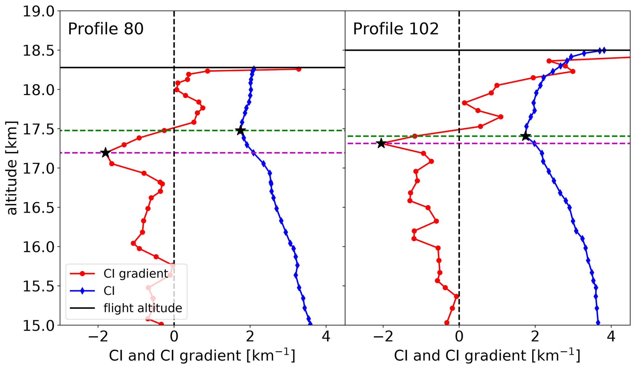
Figure 10 Altitude profiles of the cloud index (CI) and the CI gradient for two selected profiles of the CRISTA-NF measurements during RECONCILE flight 3. The CI is shown as a blue curve, and the CI gradient is shown as red curve. The flight altitude is marked by a horizontal black line. The dashed green and magenta lines show the minima of the CI and CI gradient profile respectively.

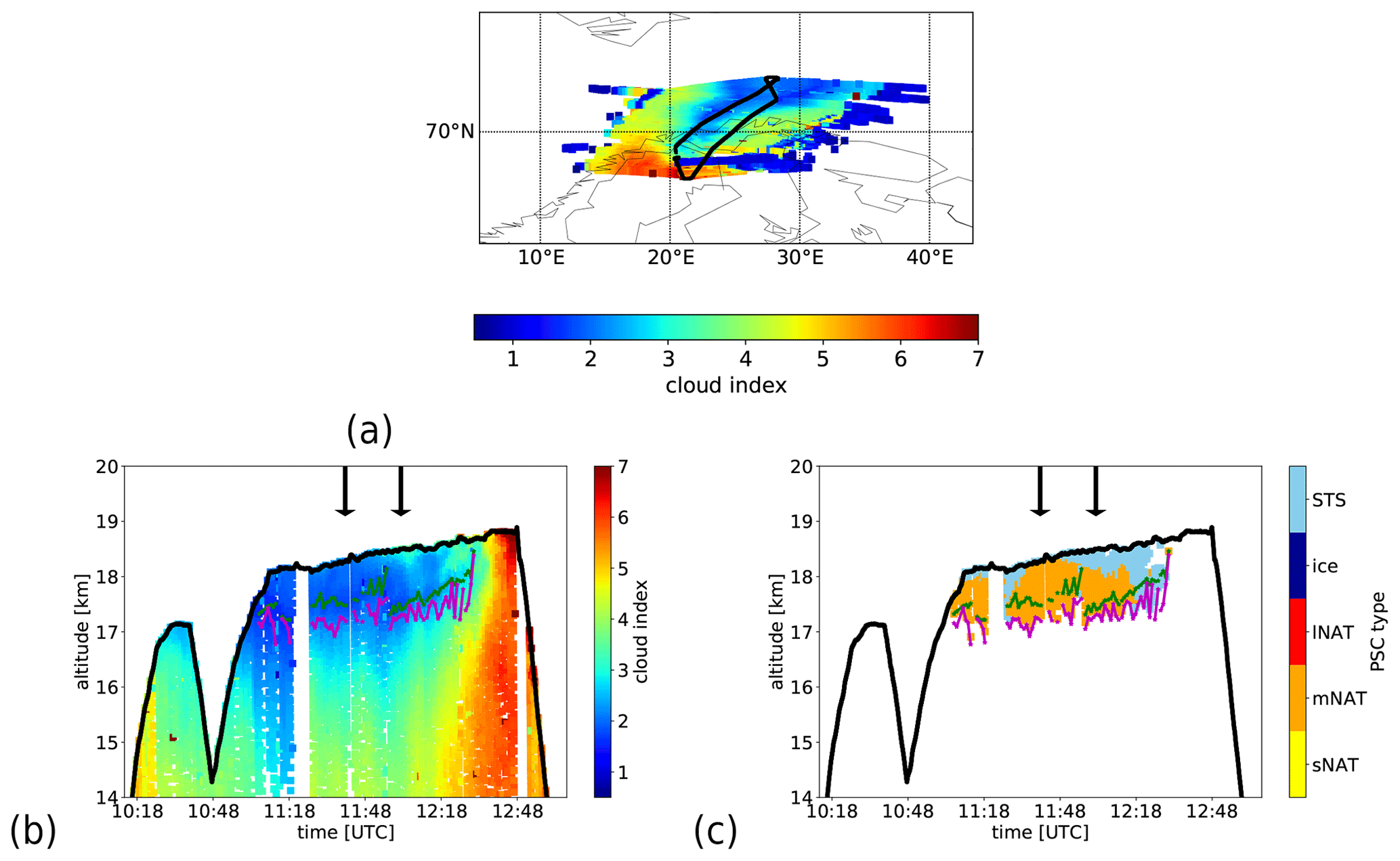
Figure 11 (a, b) Longitude–latitude and cross-section plot of the cloud index for RECONCILE flight 3. (c) Cross-section plot of the PSC types. The analysis of the PSC composition was performed for all spectra between the flight altitude and CI gradient minimum. The black line shows the flight altitude of the aircraft. The CI minimum and the CI gradient minimum are marked by a green and a magenta line respectively. Only profiles with a CI minimum below 3.0 and where both minima can sufficiently be determined are considered. The black arrows in panels (b) and (c) mark the two profiles shown in Fig. 10.

Figure 11a shows the cross section of the CI for the complete flight. During the middle section of the flight the aircraft crossed PSCs, as can be seen by the low CI values (blue colours) at and directly below the flight altitude. Beneath this region the CI values are larger again, which indicates cloud-free conditions below the PSCs. The green and the magenta line in Fig. 11a mark the CI minima and the CI gradient minima respectively. Only profiles where both minima could sufficiently be determined are considered. Similar to the results for the two selected profiles (see Fig. 10) the two minima are primarily located in the region between 17 and 17.5 km. Thus, for most profiles, a good estimate of the bottom altitude of the cloud is achieved.

4.2.2 PSC classification

During a large part of the flight, numerous spectra below the bottom altitude of the cloud (see the green and magenta lines in Fig. 11a) would be detected as PSC-influenced spectra. This is expected, as a large part of the line of sight (LOS) is still inside the PSC; thus, the spectral features caused by the PSC particles are visible in the spectra. As the cloud bottom height was determined by the CI gradient method, we restricted the analysis to the altitude range between flight altitude and the CI gradient minima. Figure 11b shows the cross section of the detected PSC types. Additionally, only spectra with a CI value below 3.0 are considered (Fig. 11b).

During the complete flight only medium sized NAT and STS were observed (orange and light blue colours in Fig. 11b). Figure 12 shows example spectra inside the PSCs at about 12:10 UTC for illustration, which show a shifted NAT feature at about 816 cm⁻¹; thus, a classification as mNAT is expected. The new method reliably detects spectra showing such a shifted NAT feature. Most of the observations detected as STS are located in the second half of the PSC observation from the flight altitude downwards. This is also in accordance with the spectra that have been measured in this region. These spectra (see Fig. 12) show a clear shifted NAT feature only at altitudes a few hundred metres below flight altitude. Directly below the flight altitude, the NAT feature can hardly be seen. This does not necessarily mean that no NAT was present in this altitude region, but the STS contribution to the measured radiances was that large that all other particle type signatures were masked out. Additionally, the CI values in this region are lower directly below flight altitude (see Fig. 11a) compared with the first part of the PSC. In addition to the smaller distance between the CI minima and the gradient minima in the second part of the PSC, this suggests that the vertical extent of the cloud is smaller compared with the first part or that the PSC is optically thinner.

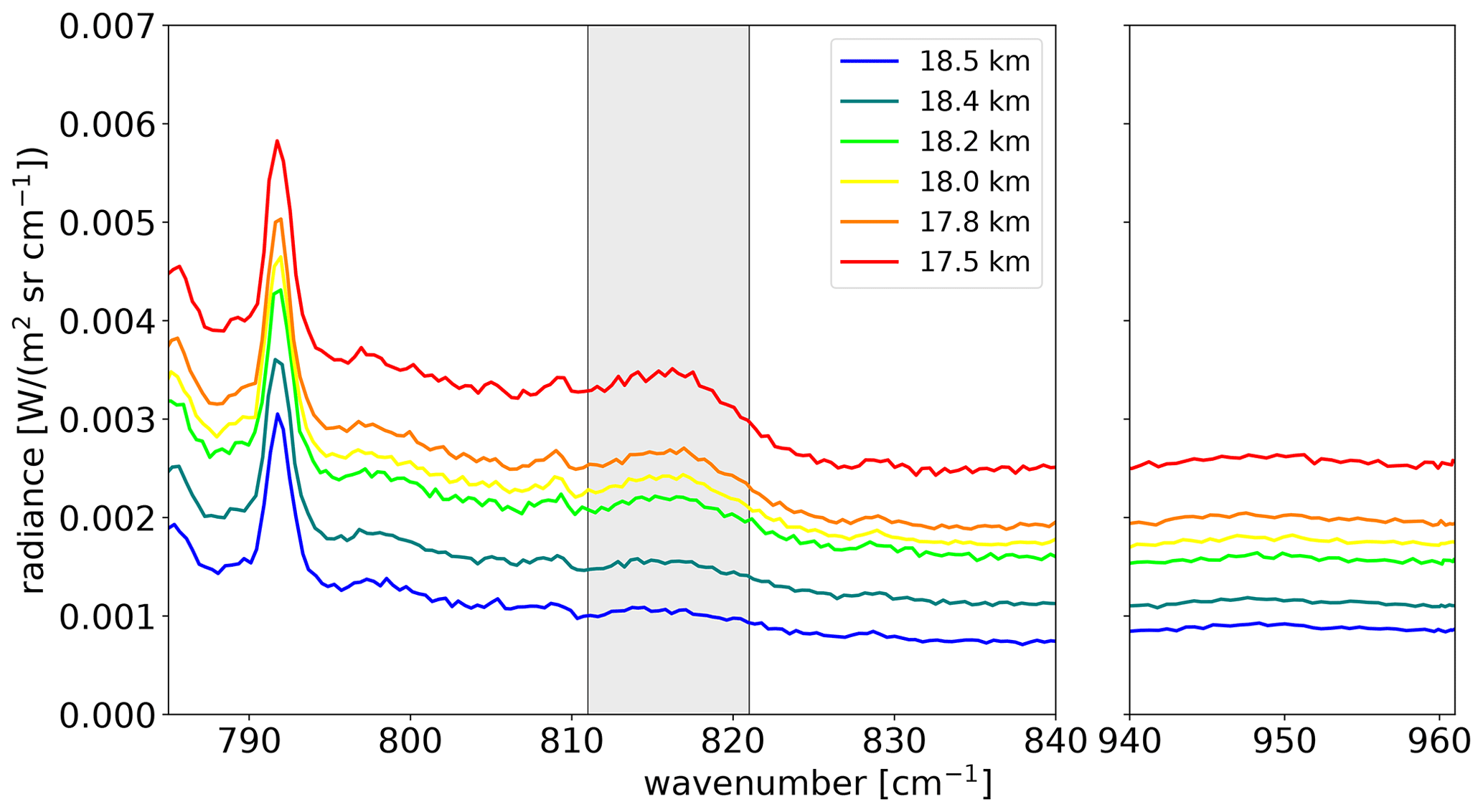
Figure 12 Example infrared spectra measured by CRISTA-NF during RECONCILE flight 3 inside PSCs at about 12:10 UTC. The spectra at different tangent altitudes are shown using colour coding. The grey bar marks the region of the shifted NAT feature.

In summary the methods derived in Sect. 3 are able to give a complete picture of the observed PSC. The PSC and the bottom altitude of the cloud are clearly detected, and the new and improved detection method enables the classification of medium-sized NAT particles and STS during RECONCILE flight 3.

5 Discussion

Small NAT particles cause a distinct spectral peak in infrared limb emission spectra at about 820 cm⁻¹. This peak has been observed in satellite measurements since the 1990s (Spang and Remedios, 2003; Höpfner et al., 2006). With our simulations, we showed that the appearance of the NAT feature changes with changing particle size. The spectral peak (small NAT) transforms to a shifted peak (medium NAT) and, finally, to a step-like behaviour of the spectrum (large NAT) with increasing median radius of the particle size distribution. This change is related to the different proportions to which scattering and emission contribute to the total radiance (see also Woiwode et al., 2016).

The change in the appearance of the feature can be used to distinguish between different size regimes. Our new approach enables the differentiation between small NAT (0.5–1.0 µm), medium NAT (1.5–4.0 µm), and large NAT (≥ 3.5 µm). As the complete analysis method is based on colour ratios, i.e. relative differences, the method searches for spectra that qualitatively show the same features as in the simulations. Possible differences concerning the absolute radiance values (e.g. influenced by vertical thickness and the optical thickness of the PSC) only lead to changes inside the correlation region for a specific particle type or size. In contrast to the former method where only one NAT index is used (detection of NAT < 3.0 µm) (see Spang and Remedios, 2003; Höpfner et al., 2006; Spang et al., 2016), this improved method leads to a larger detection capacity, as more NAT-containing clouds can be detected. A part of the medium-sized particles (those when only the NAT index-2 is above the separation line) and the complete size range of large NAT particles are not detected with the former method. This improvement will probably diminish the discrepancy between NAT cloud observations by MIPAS-Envisat and the CALIOP (Cloud-Aerosol Lidar with Orthogonal Polarization) instrument onboard CALIPSO (Cloud-Aerosol Lidar and Infrared Pathfinder Satellite Observation; Pitts et al., 2018) in the Northern Hemisphere, where much more NAT was observed by CALIOP and the agreement for the NAT observations by both instruments is only 18 % (the agreement for NAT observations in the Southern Hemisphere is much better, about 73 %) (Spang et al., 2018; Tritscher et al., 2021). Consequently, this would conclude a larger probability for the formation of NAT clouds with medium to large radii for the Northern Hemisphere compared with Southern Hemisphere conditions, which highlights a link to different formation mechanisms and meteorological conditions fostering the formation of large or small NAT particles.

The derived methods can easily be adopted to analyse other observations, such as those from MIPAS-Envisat, as the spectral behaviour is generally the same. The separation lines would need to be adjusted, because different instruments have different spectral properties and viewing geometries. Thus, the new NAT detection method can be transferred to MIPAS-Envisat, but a set of simulations is necessary to do this. In the case of the ice detection, we successfully transferred the method used for MIPAS-Envisat (e.g. Spang et al., 2016) to the airborne geometry of CRISTA-NF and refined the separation lines.

In recent publications by Woiwode et al. (2016, 2019), a special step-like behaviour of infrared spectra in the presence of NAT particles was intensively analysed, and the authors simulated the observed spectra by the presence of large aspherical NAT particles. Woiwode et al. (2019) showed the large shoulder-like signature at about 820 cm⁻¹ and flat radiance behaviour afterwards, which they called a “hockey-stick” signature, for an example observed by MIPAS-Envisat. The authors assigned this behaviour as characteristic of large aspherical NAT particles and developed a detection method for this type of spectrum. The main criteria used for the detection were a difference in the integrated radiance between the 817.5–818.5 and 833.0–834.0 cm⁻¹ windows above a certain value (to detect the step or shoulder) and a difference in the integrated radiance between the 833.0–834.0 and 960.0–961.0 cm⁻¹ windows below a certain value (to detect the flat behaviour at larger wavenumbers). Our simulations agree with the point that large spherical NAT particles (with unimodal distribution) typically show a step-like behaviour but a decrease in the radiance towards larger wavenumbers (cf. Fig. 1 reddish colours and Fig. 5b blue line) and, therefore, do not show this hockey-stick signature. However, some of our simulations for the bimodal NAT particle size distributions show this typical behaviour. The spectrum in Fig. 5 for the bimodal NAT particle size distribution (black line) exhibits no difference in radiance from about 833 to 960 cm⁻¹. Furthermore, the step or shoulder is more pronounced compared with the spectrum for the unimodal size distribution (blue line) and slightly shifted towards larger wavenumbers. Therefore, the radiance decrease from 818 to 833 cm⁻¹ increases. In our opinion, this spectrum will probably fulfil all of the criteria used for the detection of large aspherical NAT particles as described in Woiwode et al. (2019). This suggest that large aspherical NAT particles are not necessarily the only possibility to observe the kind of spectrum or spectral signature that fulfil the criteria of the detection method. Thus, the spectrum alone is possibly not enough to definitely detect aspherical NAT particles. However, a complete picture of the situation involving both infrared emission spectra, FSSP (Forward-Scattering Spectrometer Probes; Molleker et al., 2014) observations of the particle size distribution, and information on the HNO₃ budget will presumably be sufficient to make a clear decision. This has been done by Woiwode et al. (2016, 2019) for single spectra, and aspherical NAT particles led to the best results in these special cases.

As the differences used in the detection scheme by Woiwode et al. (2019) rely on absolute differences and as CRISTA-NF and MIPAS-Envisat have different viewing geometries etc., the absolute radiance values and, therefore, the differences are not comparable. Thus, the detection method cannot be applied to CRISTA-NF observations or simulations. In order to analyse the detection scheme by Woiwode et al. (2019) in more detail, simulations for the MIPAS-Envisat instrument are necessary, but this is beyond the scope of this paper. However, our simulation results demonstrate that spherical particles can qualitatively produce all the different appearances of the NAT feature (typical feature, shifted feature, step-like behaviour) in the considered spectral range, including those previously attributed to highly aspherical NAT. We think that this is an important point to consider, as it implies that IR limb emission measurements alone are not sufficient to prove the existence of aspherical NAT, in particular for cases without additional information on the atmospheric state and cloud particle size distribution. An approach using additional information about the particle size distribution and the HNO₃ budget as well as a quantitative comparison as done by Woiwode et al. (2016, 2019) would help to gain more information about particle shape. However, an approach such as this is only feasible for local case studies and not for global analyses. We do not consider our approach of grouping the NAT particles into three size bins based on the spectral signature to be affected by the particle shape, and the reasons for this are outlined in the following. The small particles (< 3 µm) are considered not or only slightly aspherical. For our approach, we used the term “small” for particle size distributions with median radii ≤ 1.0 µm. Woiwode et al. (2019) also used the method from Höpfner et al. (2006), which is based on simulations using spherical particles, to detect these small particles. Furthermore, a substantial fraction of our “medium” size group (median radii ≤ 4 µm) can be considered almost aspherical. The shifted NAT signature reported by Woiwode et al. (2016) for highly aspherical NAT is bimodal with median radii of 2 and 4.8 µm, where the latter dominates the signal. This means that the shifted NAT signature that was simulated using this bimodal size distribution in combination with aspherical particles has only been observed in the presence of larger NAT particles. Moreover, Woiwode et al. (2019) (Fig. 1) showed that a step-like NAT feature can be observed for median radii ≥ 5.0 µm. Hence, our result that the shift in the NAT signature is associated with NAT particle size is in line with the results of Woiwode et al. (2016, 2019). Due to particle asphericity, our size bin boundary between “medium” and “large” has uncertainties, and the numbers given here are valid under the assumption of spherical particles.

Grooß et al. (2014) presented a measured size distribution for a part of flight 3. The maximum in the distribution lies at a radius of about 2.5–3 µm, and a second smaller maximum at is visible about 5–6 µm. Our results for this flight show mNAT particles (1.5–4 µm). This is in a reasonable agreement considering the limits of the comparisons. Note here that the particle size distribution is observed solely at flight altitude, and CRISTA-NF observes much larger air masses. Additionally, it is likely that the larger particles are located more at lower altitudes, and the number density of these large particles will decrease with increasing altitude due to sedimentation. CRISTA-NF is also influenced by the air masses above flight altitude. Molleker et al. (2014) presented particle size distributions for flights 4 and 5. The maximum for flight 4 is at about 2.5–3 µm, and larger particles were also detected. Our results for this flight show mNAT, which is in agreement under the aforementioned restrictions for the comparison. For flight 5, different size distributions are presented that show two maxima: one at about 2.5–3 µm and a second at about 5–6 µm. This flight shows the largest amount of large particles. Our results for flight 5 show mainly mNAT and a few lNAT. This is again in agreement within the scope of the limits of the comparison. However, a detailed comparison would need additional information, such as knowledge on the vertical change in the size distribution and the vertical extent of the cloud.

6 Summary and conclusions

We performed a large set of radiative transfer simulations of infrared limb emission spectra in the presence of different types (NAT, STS, ice) of polar stratospheric clouds. All simulations were performed for the viewing geometry and spectral properties of the CRISTA-NF instrument. These simulations build a new database that is used for the analysis of PSC spectra to develop and refine detection and discrimination methods.

Our simulations showed that the NAT feature changes from a spectral peak at 820 cm⁻¹ (small NAT) to a shifted peak (medium NAT) and, finally, to a step-like behaviour of the spectrum (large NAT) with an increasing median radius. Based on this behaviour, we developed an improved method to detect NAT particles, which, for the first time, allows for the discrimination of three different size regimes under the assumption of spherical particles: small NAT (0.5–1.0 µm), medium NAT (1.5–4.0 µm), and large NAT (≥ 3.5 µm). Using colour ratios, i.e. relative differences, the method qualitatively compares observed spectra with the complete simulated database. This new detection method will also improve the analysis of other observations by infrared limb emission sounders, such as MIPAS-Envisat. The ice detection method was adopted from former studies (MIPAS-Envisat), and the separation lines were newly defined. Additionally, we developed a new method to detect the bottom altitude of the clouds. This method uses the gradient of the CI, which reaches a minimum shortly below the real bottom altitude. As the minimum of the CI itself is located inside the cloud (typically close to the bottom), these two quantities give a good estimate of the bottom altitude. This method can surely be transferred to other cloud observations, such as cirrus clouds and aerosol layers, and to other airborne instruments measuring in the same wavelength region, such as GLORIA (Gimballed Limb Observer for Radiance Imaging of the Atmosphere; Riese et al., 2014). A prerequisite for a successful usage of the method is a small FOV such as that of CRISTA-NF. Larger FOVs will lead to a larger vertical averaging of the measurements and, thus, to a reduction in the detection capabilities. This can already be seen for the CRISTA-NF instrument, where the minimum of the CI gradient can move further away from the real bottom altitude at lower altitudes (14 km and below).

Finally, we applied the new methods to observations of CRISTA-NF during the RECONCILE local flight 3. The results show a polar stratospheric cloud that has been crossed by the aircraft during the flight and extends downward to about 17–17.5 km. The PSC contained NAT particles that could be classified as medium-sized (1.5–4 µm) particles, as a shifted NAT feature was always observed in the spectra. This shifted feature is detected by the new method. Moreover, using the method developed here, a new data set of PSC observations and classification can be obtained. This new data set will help to improve the results of trace gas retrievals in the presence of PSCs by integrating realistic PSC extinction spectra into the retrieval process. Furthermore, the gained data will help to improve the representation of PSCs in model simulations.