the Creative Commons Attribution 4.0 License.
the Creative Commons Attribution 4.0 License.
 | 19 Mar 2021
Residual temperature bias effects in stratospheric species distributions from LIMS
V. Lynn Harvey
Arlin Krueger
Murali Natarajan
The Nimbus 7 Limb Infrared Monitor of the Stratosphere (LIMS) instrument operated from 25 October 1978 through 28 May 1979. Its version 6 (V6) profiles were processed and archived in 2002. We present several diagnostic examples of the quality of the V6 stratospheric species distributions based on their level 3 zonal Fourier coefficient products. In particular, we show that there are small differences in the ascending (A) minus descending (D) orbital temperature–pressure or T(p) profiles (their A−D values) that affect (A−D) species values. Systematic A−D biases in T(p) can arise from small radiance biases and/or from viewing anomalies along orbits. There can also be (A−D) differences in T(p) due to not resolving and correcting for all of the atmospheric temperature gradient along LIMS tangent view-paths. An error in T(p) affects species retrievals through (1) the Planck blackbody function in forward calculations of limb radiance that are part of the iterative retrieval algorithm of LIMS, and (2) the registration of the measured LIMS species radiance profiles in pressure altitude, mainly for the lower stratosphere. There are clear A−D differences for ozone, H2O, and HNO3 but not for NO2. Percentage differences are larger in the lower stratosphere for ozone and H2O because those species are optically thick. We evaluate V6 ozone profile biases in the upper stratosphere with the aid of comparisons against a monthly climatology of UV–ozone soundings from rocketsondes. We also provide results of time series analyses of V6 ozone, H2O, and potential vorticity for the middle stratosphere to show that their average (A+D) V6 level 3 products provide a clear picture of the evolution of those tracers during Northern Hemisphere winter. We recommend that researchers use the average V6 level 3 product for their science studies of stratospheric ozone and H2O, while keeping in mind that there are uncorrected nonlocal thermodynamic equilibrium effects in daytime ozone in the lower mesosphere and in daytime H2O in the uppermost stratosphere. We also point out that the present-day Sounding of the Atmosphere using Broadband Emission Radiometry (SABER) experiment provides measurements and retrievals of temperature and ozone that are nearly free of anomalous diurnal variations and of effects from gradients at low and middle latitudes.
- Article
(28699 KB) - Full-text XML
-
Supplement
(925 KB) - BibTeX
- EndNote


The historic Nimbus 7 Limb Infrared Monitor of the Stratosphere (LIMS) experiment provided data on the middle atmosphere from 25 October 1978 through 28 May 1979 for scientific analysis and for comparisons with atmospheric models (Gille and Russell, 1984). Remsberg et al. (2007) describe characteristics of the ozone profiles of the LIMS version 6 (V6) dataset. Notably, V6 corrects for a high ozone bias in the lowermost stratosphere of the previous version 5 (V5) profiles, as shown by comparisons of the V6 profiles with ozonesonde data in Remsberg et al. (2007, 2013). Remsberg et al. (2009) report on improvements in the profiles and distributions of V6 water vapor (H2O) within the lower stratosphere, where temperature and interfering radiances from the oxygen continuum are more accurate than in the processing of V5. Finally, Remsberg et al. (2010) contains information on the V6 improvements of nitric acid (HNO3) and nitrogen dioxide (NO2) in particular.
Frith et al. (2020) reported on modeled estimates of diurnal ozone variations, as a function of latitude, altitude, and season. In general, their modeled results are in accord with observed ozone variations from both satellite ultraviolet (UV) and microwave measurements. However, the ozone distributions from the infrared measurements of LIMS show some anomalously large day–night differences in the middle stratosphere (Remsberg et al., 1984, 2007). LIMS ozone and H2O are quite sensitive to small biases of the LIMS temperature versus pressure (or T(p)), due to nonlinear effects of the Planck blackbody function in forward radiance calculations that are part of the LIMS retrieval algorithm (Gille et al., 1984; Remsberg et al., 2004). Consequently, temperature bias is the largest source of ozone and H2O error by far, although small bias effects from T(p) are hard to verify from correlative comparisons of individual profiles. The LIMS orbital line-of-sight to its tangent layer is nearly in a meridional direction or along horizontal temperature gradients (Remsberg et al., 1990). Roewe et al. (1982) consider line-of-sight radiance gradient corrections for the LIMS species retrievals, while Gille et al. (1984) employ corrections based on the T(p) gradient. We will show that while the LIMS algorithm makes first-order corrections for T(p) gradients, residual bias effects are still apparent in the V6 species distributions.
This study considers the distributions of V6 T(p) plus plots of ascending (A) minus descending (D) orbital differences (A−D) for both temperature and species as diagnostics for the effects of residual bias errors in T(p). We evaluate those effects using plots of the LIMS level 3 (mapped) products (Remsberg et al., 1990; Remsberg and Lingenfelser, 2010) and their monthly zonal mean distributions that are part of the SPARC Data Initiative (SPARC, 2017). Section 2 gives a brief review of the characteristics and retrieval algorithms for V6 temperature and species. Section 3 reviews the measurement, retrieval, and day–night differences for temperature. Section 4 relates small temperature biases to the anomalous A−D values in the LIMS monthly species distributions for March 1979. Section 5 compares V6 daytime ozone with rocketsonde UV-filter ozone (ROCOZ) profile data for the upper stratosphere and lower mesosphere. We interpret the comparisons according to their respective error estimates and by examining the profiles in the context of hemispheric maps of the surrounding temperature and ozone fields from the level 3 products. Section 6 contains results of time series of Northern Hemisphere (NH) distributions of V6 ozone and H2O on the 850 K potential temperature surface (∼10 hPa) as indications of the quality of averages of their V6 data. Section 7 summarizes our findings about the V6 species and our recommendations for scientific studies of them. We also point out why the following experiment, Sounding of the Atmosphere using Broadband Emission Radiometry (SABER), provides measurements and retrievals of temperature that are nearly free of anomalous A−D differences at low and middle latitudes.
2.1 Daily mapped data
The V6 algorithm accounts for low-frequency spacecraft motions that affect how the LIMS instrument views the horizon and the subsequent registration of its measured radiance profiles in pressure and altitude (Remsberg et al., 2004). Retrieved ozone, temperature, and geopotential height (GPH) profiles extend from 316 to ∼0.01 hPa and have a point spacing of ∼0.88 km with a vertical resolution of ∼3.7 km. H2O, HNO3, and NO2 data are limited to the stratosphere (∼100 to 1 hPa). Processing of the original V5 T(p) profiles occurred at a rather coarse vertical point spacing of ∼1.5 km and for every ∼4∘ of latitude. Retrievals for V6 occur at every ∼1.6∘ of latitude along orbits and resolve the horizontal temperature structure better. However, the line-of-sight T(p) gradients for both the V5 and V6 processing algorithms are from daily maps of the combined V5 (A+D) temperature fields on pressure surfaces.
Mapping of the V6 profiles to a level 3 product occurs at 28 vertical levels, as opposed to just 18 levels for V5. The sequential-estimation mapping algorithm for V6 (Remsberg and Lingenfelser, 2010) employs a shorter relaxation time of about 2.5 d for its zonal wave coefficients, compared with ∼5 d for V5. The mapping algorithm is insensitive to the very few large, unscreened ozone mixing ratio values within the lower stratosphere, as noted in Remsberg et al. (2013, Fig. 1a). LIMS made measurements with a duty cycle of up to 11 d on and 1 d off, and the mapping algorithm interpolates the profile data in time to provide a continuous, 216 d set of daily zonal coefficients. Daily maps also provide a spatial context for the individual V6 profiles and are helpful for interpreting comparisons with auxiliary data sets, especially during dynamically disturbed periods.
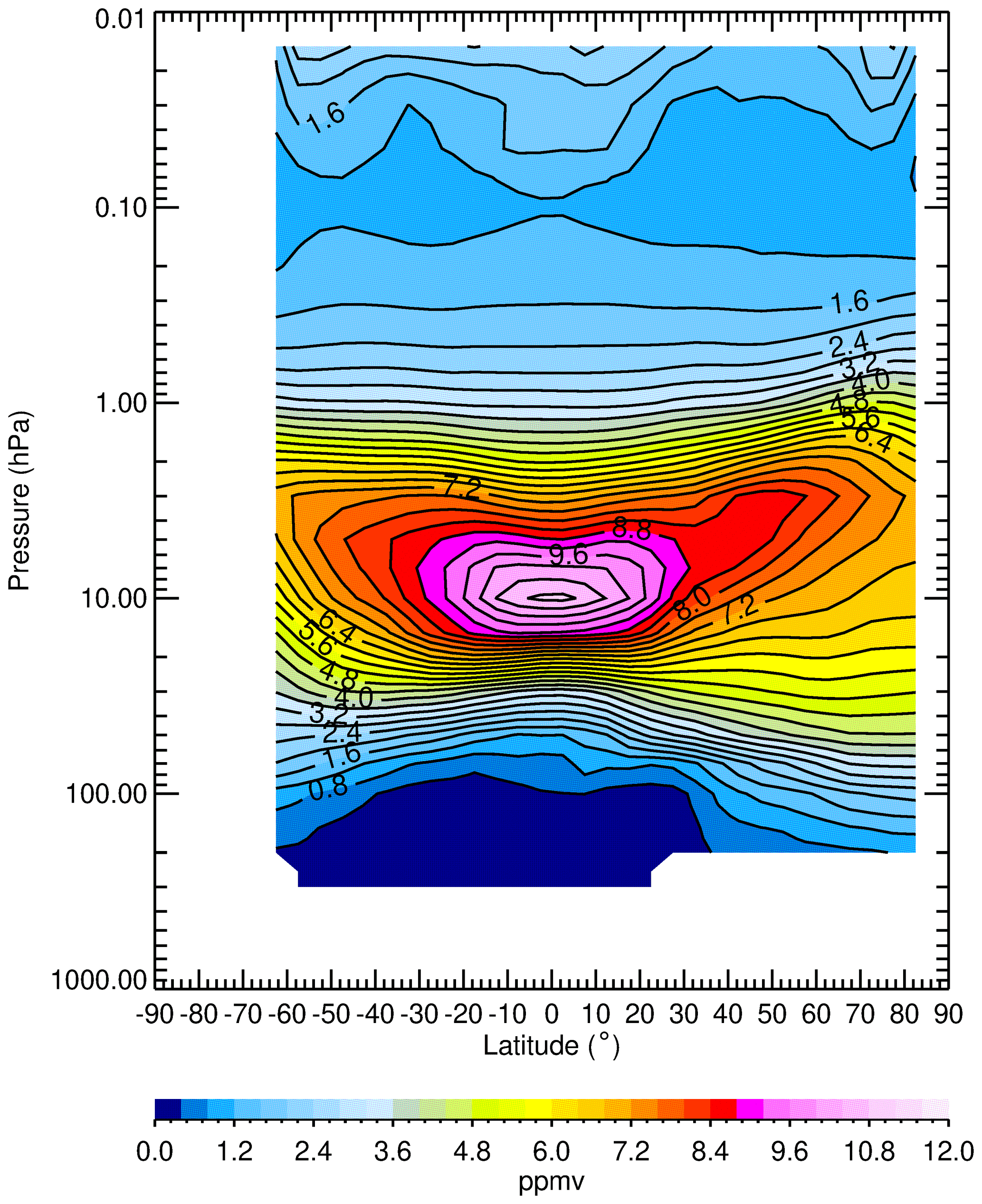
Figure 1Zonal average ozone for March 1979 from the combination of the LIMS V6 ascending and descending orbital data. Contour interval (CI) is 0.4 ppmv.
2.2 Monthly zonal average V6 ozone, temperature, and water vapor
We generated monthly zonal mean distributions from the daily level 3 files of temperature and species and supplied them to the SPARC Data Initiative or SPARC-DI (SPARC, 2017). Although the V6 ozone for SPARC-DI extends up to only the 0.1 hPa level (∼64 km), Fig. 1 updates the combined (A+D) monthly ozone for March 1979 to its highest level of about 0.015 hPa (∼75 km). Retrieved daytime ozone contributes to the (A+D) ozone in Fig. 1 and has a large positive bias throughout the mesosphere because the LIMS algorithms do not account for nonlocal thermodynamic equilibrium (NLTE) effects from either ozone (Solomon et al., 1986; Mlynczak and Drayson, 1990) or CO2 (Edwards et al., 1996; Manuilova et al., 1998). However, the V6 nighttime ozone is essentially free of those NLTE effects below about the 0.05 hPa level. We also screened the SPARC-DI product of daily zonal mean ozone values (<0.1 ppmv) near the tropical tropopause, as recommended in Remsberg et al. (2013). This study focuses on the quality of V6 ozone in the stratosphere.
Figure 1 shows that ozone has the largest mixing ratios at about 10 hPa near the Equator (∼10.8 ppmv), decreasing sharply above and below that level. Maximum mixing ratios at middle to high latitudes occur closer to 3 hPa due to larger zenith angles and longer paths of the UV light for the production of its atmospheric ozone. Remsberg et al. (2007) compared V6 ozone and Solar Backscatter UltraViolet (SBUV) version 8.0 ozone and reported that V6 ozone is larger (by 4 % to 12 %) in the upper stratosphere, although the differences are within the combined errors of V6 and SBUV. However, the monthly comparisons at 4 hPa indicate that those differences increase from November to May. Sun and Leovy (1990, their Fig. 1) also compared equatorial ozone time series from LIMS and SBUV, and they found that their monthly differences for the upper stratosphere changed with the descent of the semi-annual oscillation (SAO). Most likely, LIMS and SBUV do not resolve the vertical response of ozone to the SAO equally well.
Figure 2 shows the March zonal mean V6 T(p) distribution from SPARC-DI. Monthly T(p) extends to near the 0.01 hPa level and has values every 5∘ of latitude. T(p) has a maximum value of about 275 K at the stratopause and minimum values approaching 195 K near the mesopause and at the tropical tropopause. Radiances from the two 15 µm CO2 channels for retrievals of T(p) are free of NLTE effects below about the 0.05 hPa level (∼70 km) (Lopez-Puertas and Taylor, 2001). Estimates of a bias in V6 T(p) are in Table 1, following Remsberg et al. (2004, their Table 2, row g), but do not include any error due to temperature gradients. Estimates of bias errors for ozone due to those T(p) errors are also given in Table 1; a positive bias in temperature leads to a negative bias in retrieved ozone (and the other species) via the effect of the Planck function on radiance calculations. In principle, one may also infer the quality of the V6 temperatures based on independent estimates of the quality of the retrieved ozone. Finally, Table 1 compares V6 T(p) for March 1979 at 38∘ N with that from the temperature climatology at 40∘ N from Barnett and Corney (1985; hereafter, BC). Those (V6–BC) temperature values include a five-point running average of the SPARC-DI V6 monthly T(p) profile above the 30 hPa level to account for the broader vertical weighting functions of the satellite measurements of BC. The difference profiles, V6–BC, have values of the order of the bias estimates for V6 T(p). The larger difference of −4.4 K at 3 hPa indicates the redistribution of Northern Hemisphere temperature following the final stratospheric warming and split vortex that is specific to late February 1979.
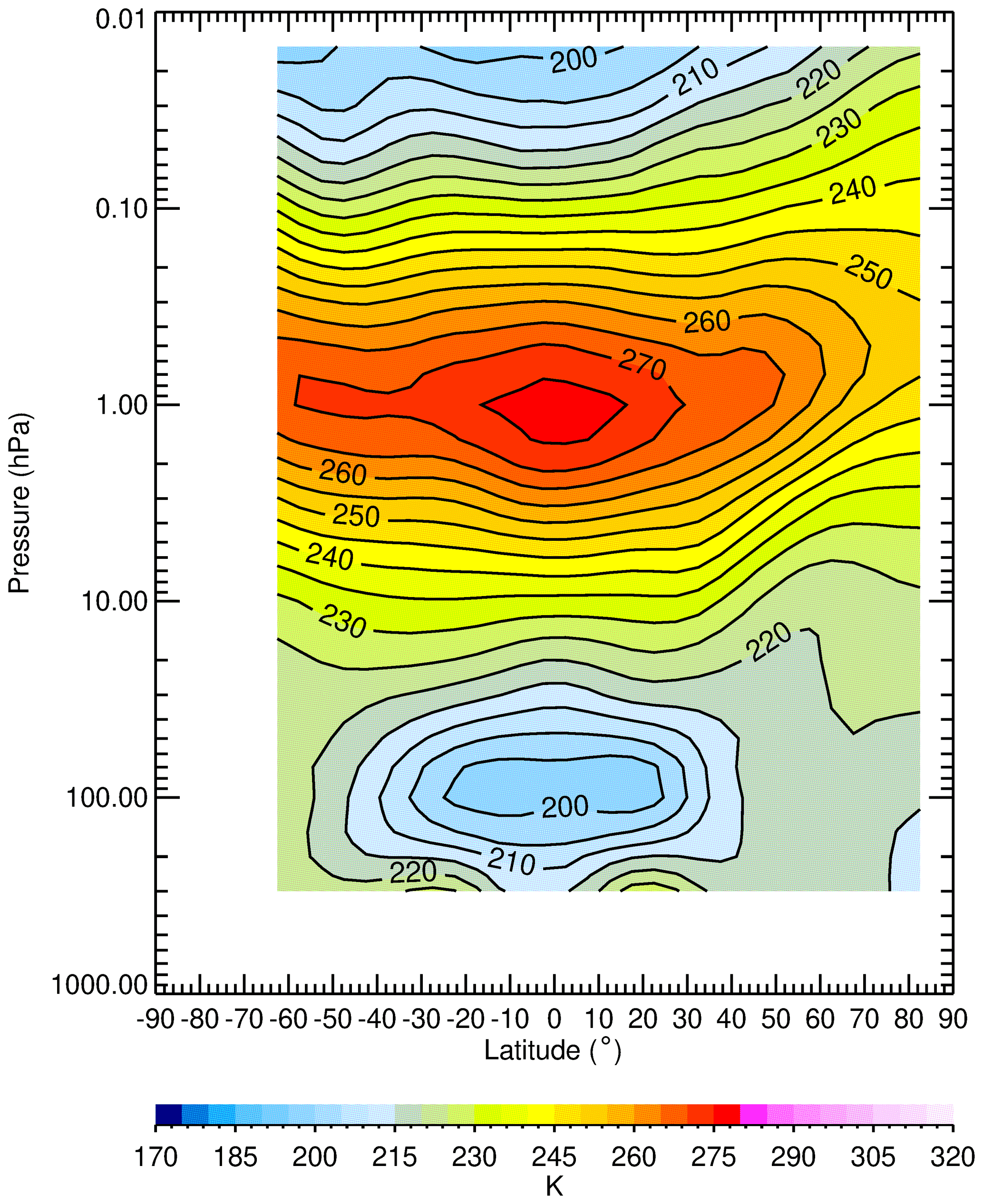
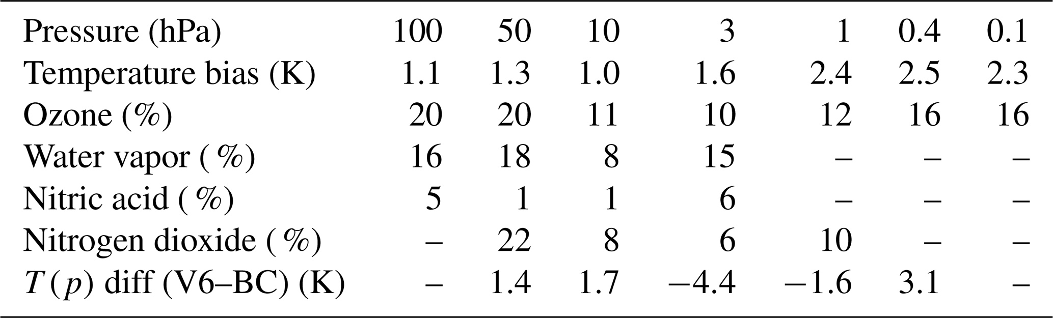
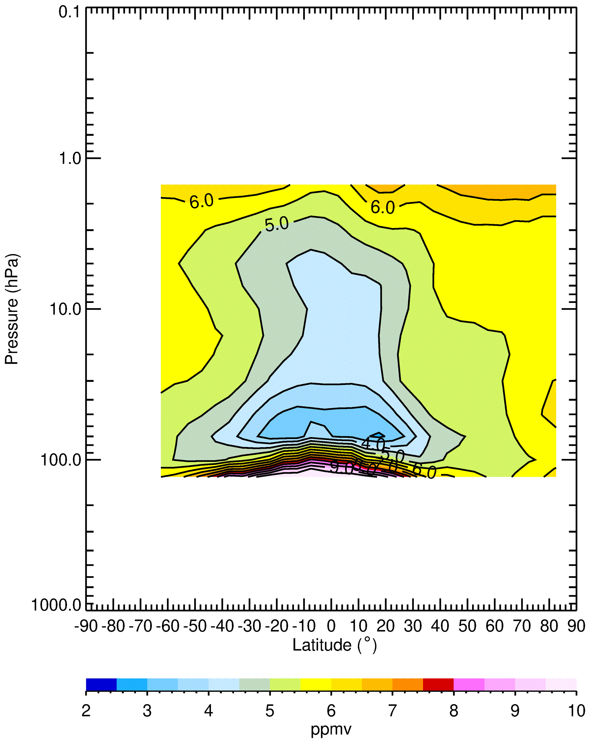
Figure 3 shows V6 zonal average H2O for March 1979 from SPARC-DI. The highest values of H2O are at upper altitudes (>6.0 ppmv) and are due to the oxidation of methane (CH4) to H2O, followed by its net transport and accumulation at higher latitudes. H2O is effectively a tracer of the mean meridional circulation, which moves upward from the tropical tropopause to the middle stratosphere and then poleward toward higher latitudes. Minimum zonal-mean values of H2O are of the order 3.5 ppmv in the tropics between 50 and 70 hPa. The sharply increasing H2O near the tropical tropopause may be due in part to residual radiance from cirrus cloud tops. The V6 species have a first-order screening for clouds at latitudes between ±30∘ and for pressure altitudes below 45 hPa, according to a threshold criterion of the vertical slope of the co-located ozone mixing ratio profiles (see Sects. 2.2 in Remsberg et al., 2007, 2009). Locations of cloud tops are in separate daily files that are a part of the V6 level 2 or daily profile data set. NLTE processes also cause enhancements of H2O radiance near the stratopause during daytime. Those uncorrected NLTE effects extend downward to lower altitudes for retrieved V6 H2O, although the effects are small for the middle and lower stratosphere (Mertens et al., 2002). Estimates of the effect of temperature bias for V6 H2O are in Table 1 of Remsberg et al. (2009).
Nimbus 7 was in a near-polar orbit, and LIMS made measurements at around 13:00 LT (local time) along its ascending (A or south-to-north traveling) orbital segments and at 23:00 LT for its descending (D or north-to-south traveling) segments. The A−D time difference is of the order of 10 h because LIMS viewed the atmosphere 146.5∘ clockwise of the spacecraft velocity vector or 33.5∘ counterclockwise from its negative velocity vector, as seen from overhead. In other words, LIMS viewed atmospheric tangent layers in opposing meridional directions for the NH and through the tropics or toward the SSE along A segments and toward the NNW along D segments (Gille et al., 1984; Remsberg et al., 1990). The A and D view paths for middle latitudes of the Southern Hemisphere (SH) are nearly in a zonal direction and toward the NNW, respectively, due to the orbital inclination of Nimbus 7.
Figure 4 shows V6 A−D temperatures for March. The differences of the upper stratosphere indicate how well the effects of the temperature tides have been resolved (Remsberg et al., 2004). Tropical differences are due mainly to diurnal tides, and they become large in the mesosphere. Tidal variations for the tropics increase with altitude in Fig. 4, ranging from −2 K at 15 hPa to +4 K at 1.5 hPa. They agree qualitatively with ones from rocket datasonde profiles (Hitchman and Leovy, 1985; Finger et al., 1975). Figure 4 also shows the expected 180∘ change of tidal phase for A−D T(p) from the tropics to the subtropics. Accurate determinations of T(p) versus latitude depend critically on knowledge of the Nimbus 7 spacecraft attitude. That information for a complete orbit comes empirically from profiles of calculated-to-measured radiance ratios for the LIMS narrow CO2 channel and can lead to a bias error for A−D T(p). Although orbital attitude bias will affect T(p) at all altitudes, that error source is small according to the good comparisons of the LIMS-derived geopotential heights versus those from operational analyses at both the 10 and 46 hPa levels (Remsberg et al., 2004). Even so, Fig. 4 also shows that there are residual A−D T(p) differences at 70 hPa that are opposite in sign at 40∘ S and 30∘ N, or just where there are large, opposing meridional gradients in T(p) in Fig. 2.
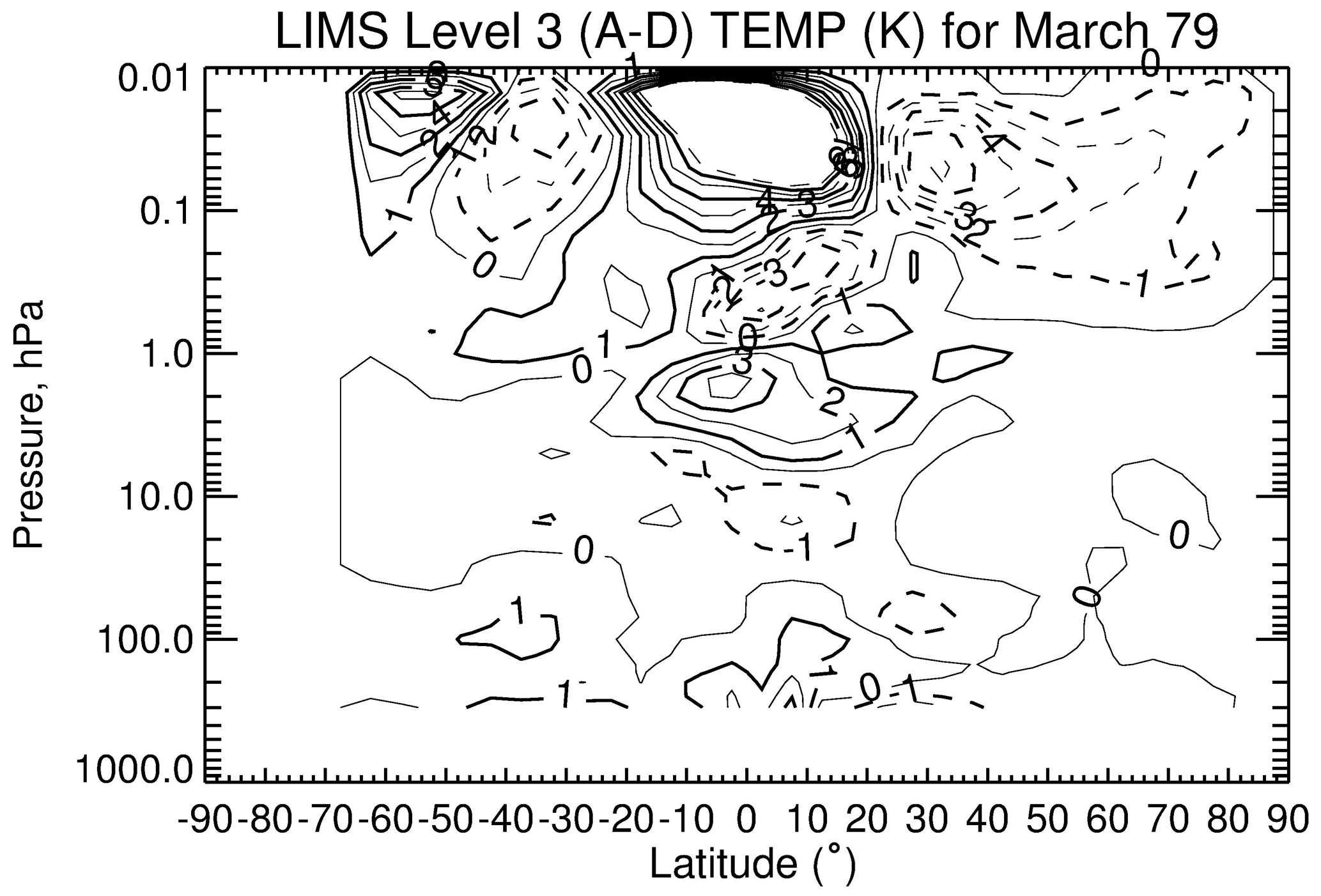
Figure 4LIMS V6 level 3 ascending minus descending (A−D) temperature differences (in K) for March 1979. CI is 1 K, and solid contours show positive differences.
Measured ozone radiance profiles contain the full effects of any atmospheric variations in T(p). As an example, Fig. 5 shows zonal mean ozone radiance differences (A−D) for 1 d (15 March 1979). Radiance differences in the tropics have a change in sign from positive at 3 hPa to negative in the lower mesosphere, and they correspond directly with the A−D changes of temperature in Fig. 4. Positive A−D radiances at middle latitudes of the lower mesosphere are due to the dominance of NLTE daytime radiances from CO2 and O3, as compared with the tidal effects from T(p).
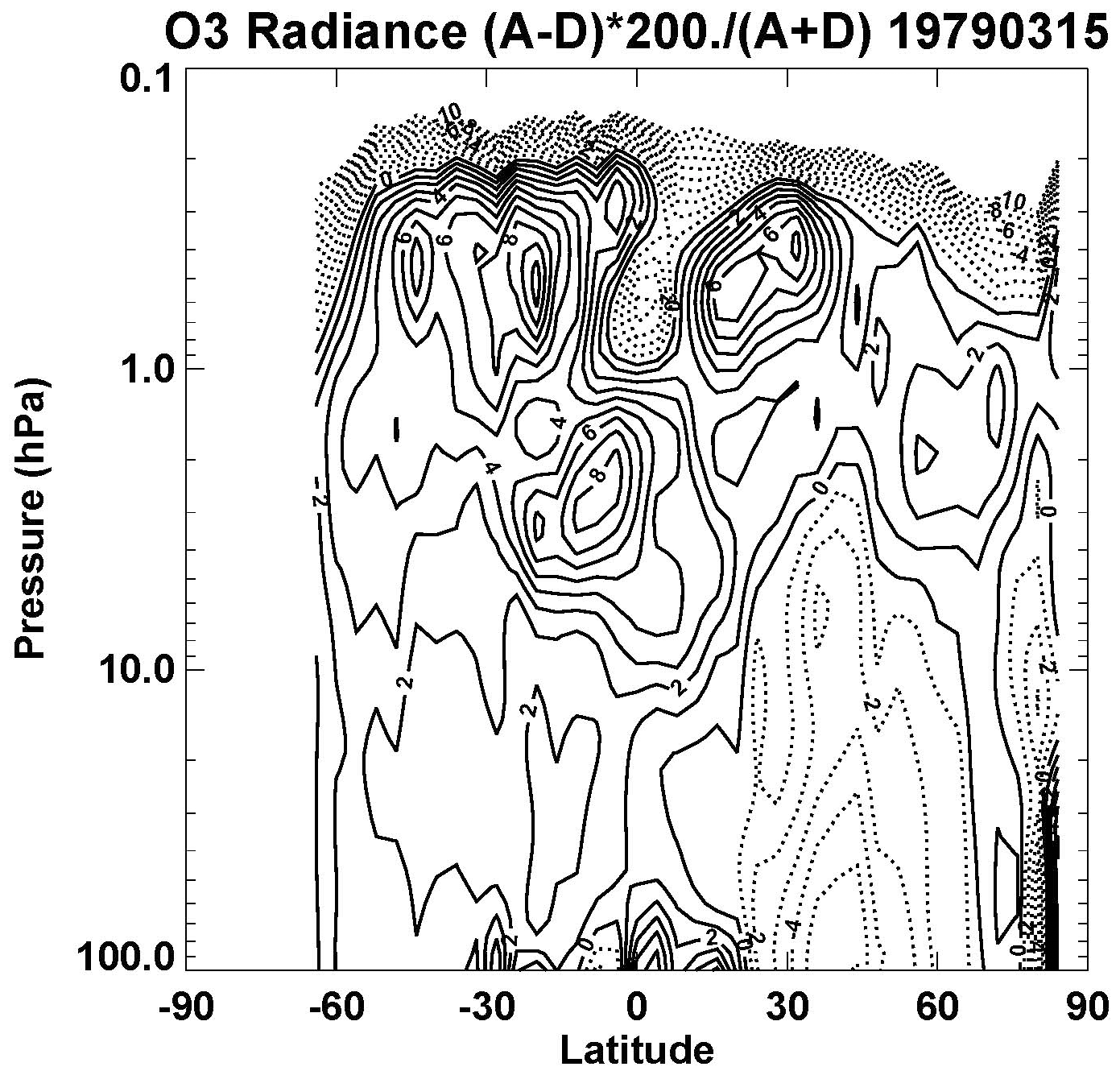
Figure 5Ascending minus descending ozone radiance differences (in %) for 15 March 1979. Contour interval is 1 %.
There are negative A−D ozone radiances of up to −5 % at the northern middle latitudes of the stratosphere, and they are a result of the meridional decrease of T(p) (in Fig. 2) from the northern subtropics toward higher latitudes. More of the measured radiance in that region comes from the front end of the tangent layer or from the colder side of the A orbital segment and from the warmer side of the D segment, leading to negative A−D radiances. Gille et al. (1984) found that the corresponding A−D temperature differences extend to 4 K or even greater at high northern latitudes. The LIMS algorithms for temperature and species account for horizontal temperature gradients on a pressure surface in the following manner. Daily near-global temperature fields were obtained from a mapping of the T(p) profiles from a V5 first-pass retrieval. The mapped fields are at 18 separate pressure levels (spaced vertically by 2.3 to 4.3 km, depending on level). Temperature gradients for each profile were determined from the maps, according to the LIMS tangent path viewing direction in longitude and latitude, and new second-pass T(p) retrievals were performed taking account of those gradients. V5 gradient estimates from the similar V5 level 3 map product were used for the processing of the V6 profiles. The T(p) gradient values for each profile are on the archived V6 level 2 files and used for retrievals of the species. While both the V5 and V6 temperature profile biases become smaller after gradient correction, one must remember that our analyzed temperature gradient information is approximate.
The A−D T(p) differences may still be on the order of 1 to 2 K after correction (see Figs. 4 and 5 in Gille et al., 1984; Remsberg et al., 2004, 2007). Kiefer et al. (2010) analyzed for the effects of a T(p) gradient in more detail using data from the limb-infrared, Michelson Interferometer for Passive Atmospheric Sounding (MIPAS) experiment. They confirm the need to correct for T(p) gradients in the respective A and D views for accurate retrievals of species from the MIPAS A and D radiance profiles. We emphasize that the T(p) gradients for LIMS V6 are from daily surface maps of average (A+D) V5 temperature fields, where the meridional resolution of the V5 fields is no better than half that of V6 or 4∘ versus 2∘ of latitude. Those V5 average (A+D) T(p) gradients underestimate the true atmospheric gradients and can result in slight biases between the A and D T(p) values for V6 at a given latitude.
V6 retrievals of T(p) employ a starting reference pressure level Po near 20 hPa (∼ 26 km relative altitude) plus hydrostatic conversions to pressure altitude that extend both upward and downward from Po. The algorithm makes forward radiance calculations for the two broadband CO2 channels and compares them with their measured radiance profiles. T(p) (A−D) differences of the same sign will impart growing A−D radiance versus pressure differences away from Po. Both Po and T(p) undergo iteration until the calculated and measured tangent layer radiances agree to within the noise levels of the measured radiances over the pressure range of 2 to 20 hPa. However, the noise value is nearly 2 % of the signal at 2 hPa for the narrow CO2 channel. This pressure level is where the diurnal temperature tide has a larger amplitude and can impart a systematic A−D bias in Po. A−D bias errors in radiance versus pressure are also significant; a radiance calibration error of 1 % causes a 0.6 K error in T(p) for the middle and upper stratosphere (Remsberg et al., 2004, Table 3). Another possible source of (A−D) bias for T(p) can arise from a residual uncertainty of the viewing attitude of LIMS along an orbit, its empirical “twist factor”.
Roewe et al. (1982) showed that adjustments for horizontal gradients in T(p) affect species retrievals through calculations of the Planck blackbody radiance, as well as from the registration of their radiance versus pressure profiles, mainly in the lower stratosphere. The region of negative A−D ozone channel radiance in Fig. 5 has values that increase toward the lower stratosphere because of persistent A−D T(p) biases plus the hydrostatic registration of the measured radiance profiles with pressure altitude. The radiance differences are negative at middle latitudes of the NH but positive in the SH. Ozone radiance at 10 hPa (not shown) increases from 40 to 18∘ N, holds nearly steady in the tropics, and decreases from 20 to 40∘ S, mainly due to the changing ozone with latitude (Fig. 1). Gordley and Russell (1981) showed that the bulk of the LIMS broadband ozone radiance for the middle and lower stratosphere comes from the near side of the tangent layer (displaced toward the satellite by about 300 to 500 km or ∼3 to 6∘ of latitude). That tangent layer weighting explains part of the observed change of sign of the A−D radiances between the two hemispheres in Fig. 5. Nevertheless, the mass path algorithm of the V6 forward model simulates radiance along a well-resolved limb path, using rigorous ray-tracing methods, including refraction effects and the first-order corrections for temperature gradients, and assigns an observed tangent altitude corresponding to the center of the measurement field-of-view.
Roewe et al. (1982) also showed that adjustments for the path gradients of the ozone mixing ratio itself imparts only small A−D mixing ratio differences (∼2 %). Thus, V6 retrievals do not account for species gradients. The V6 algorithms are no longer operational for further detailed studies of the effects of T(p) gradients for the LIMS species. Instead, in the next section we present diagnostic plots based on the V6 level 3 data themselves to indicate that there are residual biases in the distributions of V6 T(p) and that they carry over to the V6 species.
4.1 Upper stratospheric ozone and H2O
Remsberg et al. (1984, 2007) reported on the occurrence of day and night or the A−D ozone values, and they are similar for V5 and V6. Figure 6 shows the distribution of V6 A−D ozone for March as divided by the zonal mean ozone, such that the pattern of systematic differences is a percentage of the zonal average ozone. Photochemical calculations by Haigh and Pyle (1982) predict about a −2 % change in ozone for a +1 K change in T(p) at 1.5 hPa. The V6 tropical ozone differences in Fig. 6 grow to nearly −3 % near 1 hPa and are opposite in sign to the temperature tides of Fig. 4. Thus, the V6 ozone of the tropical upper stratosphere agrees reasonably with effects from the observed temperature tides.
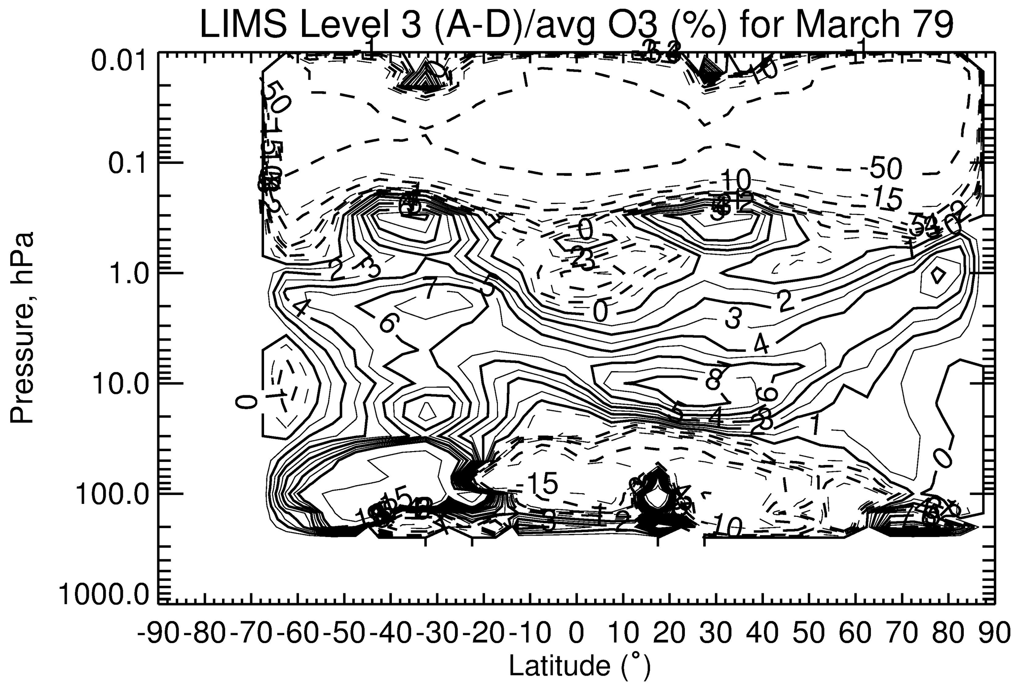
Figure 6LIMS V6 level 3 monthly zonal mean (A−D) ozone differences divided by average ozone (and given in %) for March 1979. Solid contours are positive and CI is 1 % from 0 to 10, 5 % from 10 to 15, and then skips to the 50 % contour.
Sakazaki et al. (2013, their Fig. 4) also reported diurnal model calculations of tropical day–night ozone values of −3.5 % at 44 km (∼1.7 hPa) at the local times of the LIMS observations; their microwave observations of ozone agree with them. They also obtained A−D ozone variations of +3.5 % at 34 km (∼6 hPa) from the photochemistry of odd oxygen during daytime, and those differences decay away from the Equator. However, the V6 A−D tropical ozone differences of Fig. 6 are nearly twice as large at 6 hPa, and they disagree with modeled changes in Frith et al. (2020). There are also separate rather large V6 ozone differences at middle latitudes of the upper stratosphere, where effects from temperature tides are small. The rather large A−D ozone values (∼4 % to 6 %) at SH middle latitudes correspond to where the A−D ozone radiances in Fig. 5 are increasing with altitude by +2 % to +4 % and where A−D T(p) is weakly negative. While these results are consistent with the effects of temperature on retrieved ozone through the V6 algorithm, the ozone radiances may also have an A−D pressure registration bias due to the persistently negative A−D T(p) in that region. The axis of the positive A−D ozone anomaly at NH middle latitudes in Fig. 6 overlays the region of rather large meridional T(p) gradients in Fig. 2.
Figures 7 and 8 provide supporting evidence that uncorrected, residual temperature gradients are a likely cause of the A−D ozone anomalies in Fig. 6. Figure 7 shows zonal (wave) standard deviations (SD) about the zonal average of the combined (A+D) temperature fields for March, where the SD values are from the LIMS SPARC-DI data product. There is significant zonal wave activity at middle to high latitudes in both the NH and SH, and one must account for their separate A and D horizontal gradients for accurate ozone retrievals. Figure 8 shows the corresponding zonal wave standard deviations for ozone that have a maximum value of 0.40 ppmv near 65∘ N and 1 hPa or where transport affects the ozone as well as chemistry.
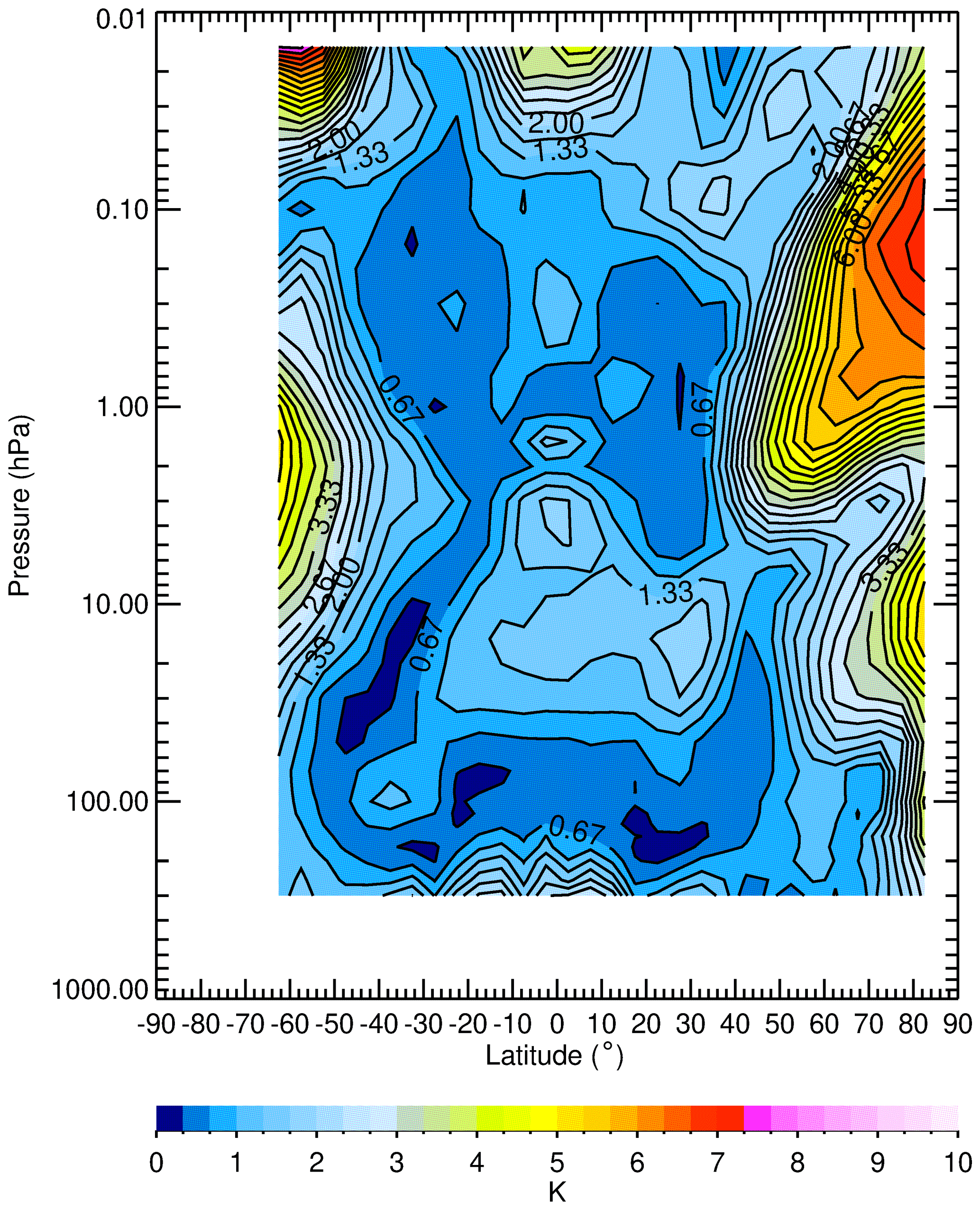
Figure 7Average zonal (wave) standard deviation of temperature for March 1979. Contour interval is 0.33 K.
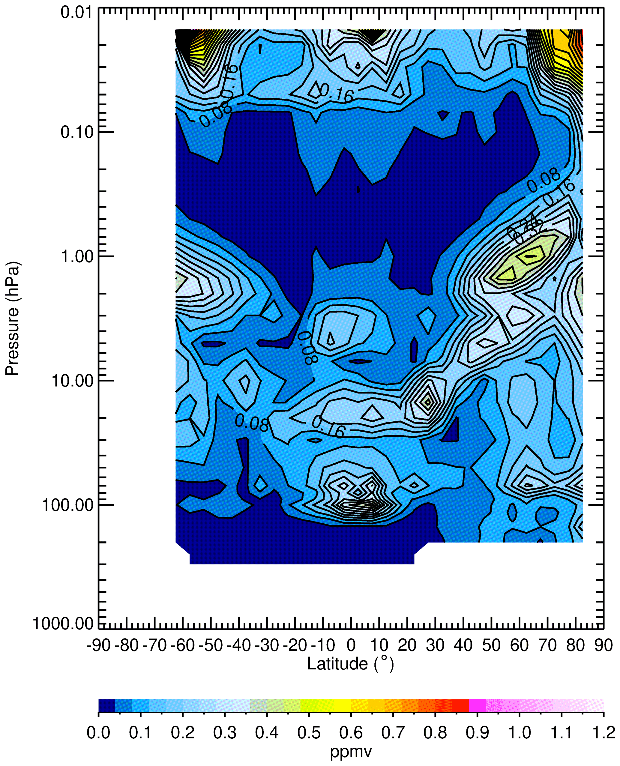
Figure 8Average zonal (wave) standard deviation of ozone for March 1979. Contour interval is 0.04 ppmv.
V6 H2O retrievals are more sensitive than ozone to biases in T(p) at 3 hPa (in Table 1) because most of the V6 H2O radiance comes from its strong nearly saturated lines. Figure 9 shows H2O A−D mixing ratio values for March. Both species are altered by horizontal gradients in T(p) in the same way in calculations of their Planck radiances. The locus of maximum percentage difference for H2O in the SH middle to upper stratosphere differs from that for ozone (Fig. 6) because their respective mixing ratios also have gradients that differ. The effect of the tropical temperature tide on H2O is not apparent at 1.5 hPa because of the excess of NLTE radiance for V6 daytime H2O at and above that level.
Figure 9LIMS V6 level 3 ascending minus descending (A−D) H2O differences divided by average H2O (and given in %) for March 1979. CI is 1 % from 0 to 10 and then 5 % from 10 to 15; solid contours show positive differences.
4.2 Middle and lower stratosphere ozone and H2O
V6 A−D ozone mixing ratio in Fig. 6 is near zero at 20 hPa. This feature occurs where V6 A−D for T(p) in Fig. 4 is also small, or where there is iteration of Po and a hydrostatic integration both above and below that level. The ozone differences become negative below that level across the tropics and in the NH, where the vertical gradient of ozone (Fig. 2) is large and subject to small A−D differences for the registration of the ozone radiance profiles. However, the ozone differences at SH middle latitudes remain positive down to the 100 hPa level; only tangent views along the descending orbital path are in a nearly meridional direction at those latitudes. In particular, the A−D ozone values in Fig. 6 are rather large at 40∘ S and at 30∘ N (40 to 100 hPa), and they are opposite in sign to the A−D T(p) differences of order ±1 K in Fig. 4. This finding agrees with the estimates of T(p) effects at 50 hPa in Table 1, where a bias of −1.3 K leads to a +20 % bias in ozone. The A−D temperature biases are large only where the meridional temperature gradients are also large (Fig. 2) and where corrections for them may be too small.
A−D values for H2O in Fig. 9 have an opposite character from those of ozone from 50 to 100 hPa because the vertical gradient of H2O in Fig. 3 is also opposite that of ozone in the lowermost stratosphere. This finding is a clear indication of how the same A−D T(p) biases can affect retrieved ozone and H2O differently. The few correlative balloon measurements of H2O during 1978 and 1979 are too uncertain to judge whether the V6 H2O A or D profiles are more accurate.
One particular feature is that both A−D ozone and H2O are positive and approach 8 % at about 10 hPa and 25∘ N. The SD values for temperature and ozone show local increases there as well. Figure 10 gives details about the NH distribution of V6 ozone on the 10 hPa surface for 1 d, 15 March 1979, from a gridding (at 2∘ lat, 5.625∘ long) of its 13 zonal Fourier coefficients (a zonal mean and 6 cosine and sine values) in the level 3 product (Remsberg and Lingenfelser, 2010). There is a meridional ozone gradient at the equatorward edge (∼25∘ N) of a much larger middle-latitude region of near-zero gradient – a result of effects of an efficient mixing with air from higher latitudes during late winter. Zonal average A−D temperatures at 10 hPa in Fig. 4 are on the order of −1 K at 15∘ N but then change to weakly positive at 25∘ N. The corresponding NH field of T(p) on 15 March is in Fig. 11, and it shows a narrow belt of slightly higher temperature near 25∘ N or where the A−D meridional T(p) gradient changes sign in Fig. 4. Such small T(p) differences also affect the registration of the ozone and H2O radiance profiles. There are unexpected tropical A−D ozone mixing ratios on the order of 5 % at 10 hPa for all the LIMS months. Those anomalies appear to migrate seasonally across the tropics and subtropics (see temperature and ozone results for other selected months in the Supplement).
Figure 10V6 ozone at 10 hPa for 15 March 1979 in the NH. Ozone contour interval is 0.5 ppmv, and latitude spacing (dotted circles) is 10∘.
4.3 Stratospheric HNO3 and NO2
LIMS HNO3 is optically thin and its retrievals are much less sensitive to temperature bias via the blackbody function (Table 1). Its radiance profile measurements also come more from the center of the tangent layer, unlike those of ozone and water vapor. Maximum mixing ratios for HNO3 occur at about 20 hPa in the tropics and 30 hPa at high latitudes (e.g., as in Fig. 1 of Remsberg et al., 2010) or similar to those of ozone. Figure 12 is a plot of A−D for V6 HNO3 (in %) for March for comparison with that of ozone in Fig. 6, and there are two important differences between them. First, A−D for HNO3 in the middle and upper stratosphere is uniformly negative due to its photolysis during daytime, whereas A−D for ozone is slightly positive from enhanced production during the day. Secondly, there are no apparent variations in A−D for HNO3 in the upper stratosphere at 40∘ S and near 10 hPa at 25∘ N from the effects of co-located, horizontal temperature gradients. However, the patterns with latitude of A−D in the lower stratosphere are very similar for both HNO3 and ozone and indicate the effects of A−D temperatures on the registration of the radiance profiles prior to their retrieval to mixing ratios.
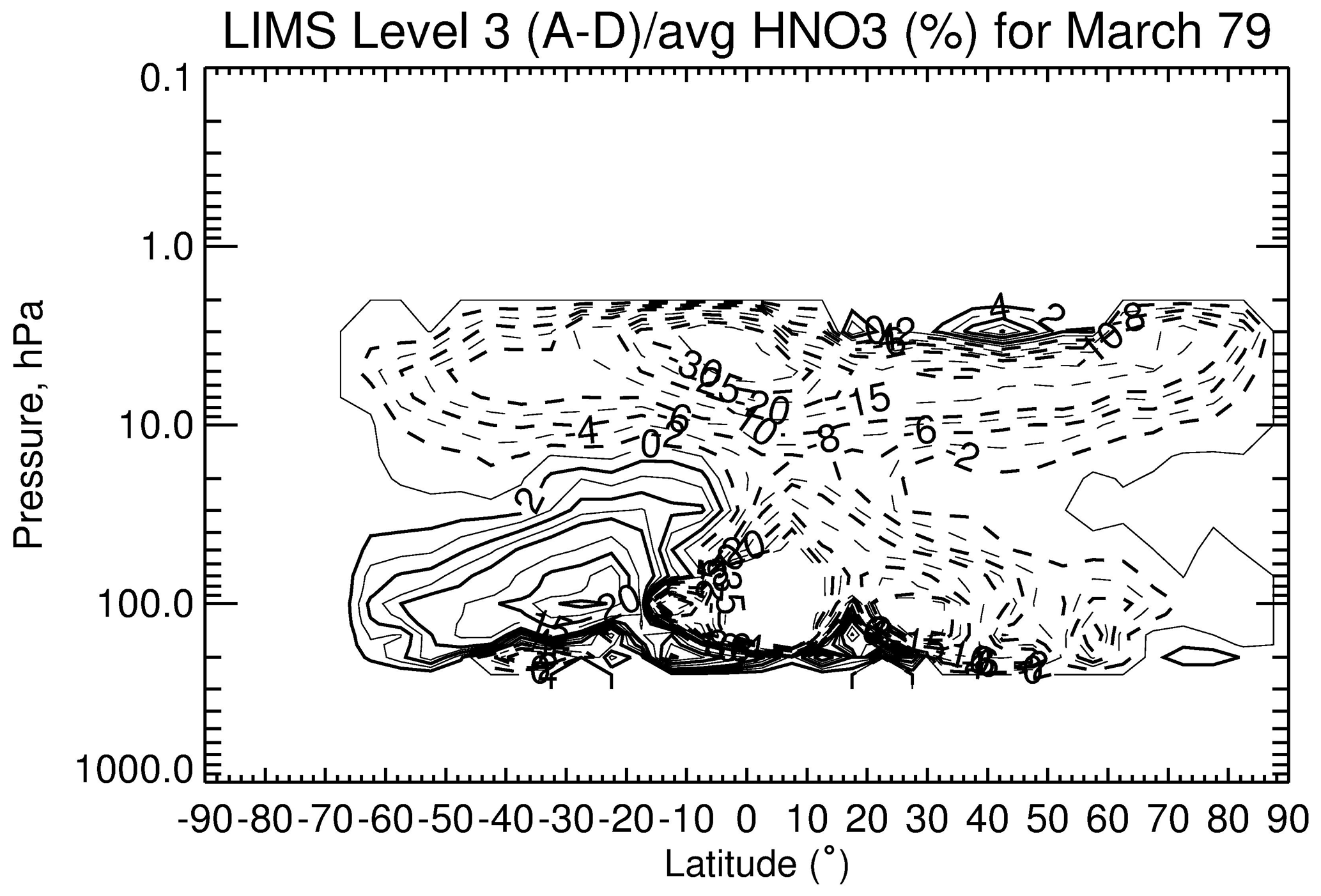
Figure 12LIMS V6 level 3 ascending minus descending (A−D) HNO3 differences divided by average HNO3 (and given in %) for March 1979. CI is 2 % from 0 to 10 and then 5 % from 10 to 35; solid contours show positive differences.
LIMS measured NO2 radiances at around 13:00 and 23:00 LT from the Equator to 60∘ N but changed quickly to 14:45 and 21:18 LT by 80∘ N. There is a more gradual change in viewing times for the Southern Hemisphere from 13:23 to 22:37 LT at 20∘ S and then from 15:45 and 20:15 LT at 60∘ S, all due to the orbital viewing geometry of LIMS. V6 NO2 mixing ratios decrease rapidly after sunrise and then increase sharply again at sunset. There is also a slow conversion of NO2 to NO3 and N2O5 after sunset, mainly in the middle stratosphere (Brasseur and Solomon, 2005). Figure 13 shows a slightly different but more standard diagnostic of NO2 A to D ratios for March, and they vary according to the local times of the measurements. However, note that the LIMS observations occurred beyond the day–night terminator at the highest latitudes. V6 NO2 has low below about the 30 hPa level and is not accurate there; elsewhere the A to D ratios should be representative.
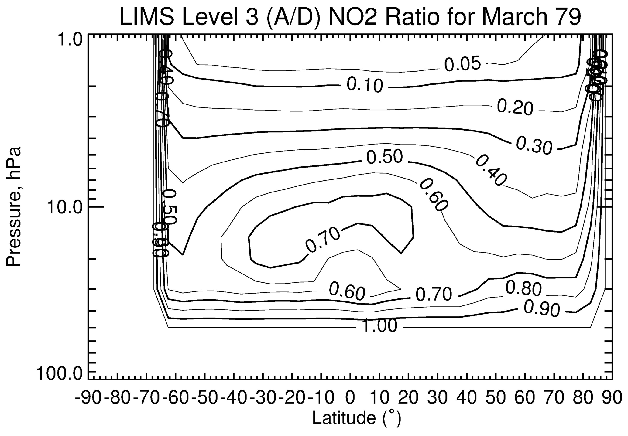
Figure 13Distribution of the A to D ratios of V6 NO2 for March 1979. CI is 0.05 (from 0.0 to 0.1) and then 0.1 (from 0.1 to 1.0).
V6 NO2 is also sensitive to temperature bias (Table 1 and Remsberg et al., 2010). Figure 13 shows a slight asymmetry of the 0.7 contour about the Equator; these ratios are smaller in the northern subtropics or opposite in magnitude to that expected from the effects of the T(p) bias in Fig. 4. There is significant interfering radiance from H2O in the NO2 channel from the middle to lower stratosphere (Russell et al., 1984); recall that H2O has its own T(p) bias effects (see Fig. 9). Radiance from H2O is also a larger correction for day versus night V6 NO2. Thus, although we expected to find temperature bias effects in V6 NO2, indications of them are somewhat ambiguous in Fig. 13.
This section considers the quality of the V6 ascending (daytime) ozone of the middle and upper stratosphere at NH middle latitudes; there is only one corresponding comparison for the descending (nighttime) ozone (not shown, but see Remsberg et al., 1984, their Fig. 13). Krueger (1973) developed meteorological rocket-borne, UV-absorption ozonesonde (ROCOZ) instruments in the 1960s and 1970s and made routine soundings of middle atmosphere ozone. To measure absorption of sunlight in three altitude regions between 15 and 60 km, ROCOZ used four interference filters procured commercially in batches for uniformity. There were launches of ROCOZ instruments for the validation of LIMS (seven flights) and of SBUV ozone at low latitudes (Natal, Brazil), middle latitudes (Wallops Island, VA) and high latitudes (Fort Churchill and Primrose Lake, Canada). Remsberg et al. (1984) reported on comparisons of the V5 ozone with ROCOZ soundings and found mean differences (V5 minus ROCOZ) that varied from 5 % in the upper stratosphere to 16 % in the lower stratosphere. The rms differences were rather large though (12 % to 23 %, respectively), and there were concerns about the stability of the batch of UV interference filters used in the ROCOZ instruments from late 1978 through mid-1979.
An early “ozone climatology” was produced from the greater than 200 ROCOZ soundings launched between 1965 and 1990 at rocket ranges from the Equator to high latitudes of both hemispheres (Krueger, 1984; WOUDC, 2021). The ROCOZ flights include a SH latitude survey, calibration flights for the Orbital Geophysical Observatory (OGO-4) UV spectrometer (London et al., 1977), low-latitude baseline flights from Antigua, high-latitude flights from Fort Churchill and Primrose Lake, validation flights for the Backscatter Ultraviolet (BUV) experiment on Nimbus 4, and a regular monthly series of measurements from Wallops Island, VA. In fact, the 1976 U.S. Standard Atmosphere middle-latitude ozone model makes use of rocket data from seven international experimenters, including ROCOZ (Krueger and Minzner, 1976).
Krueger (1984) also compiled separate monthly averages of soundings from Wallops Island (38∘ N) during the period of March 1976 through September 1978. Uncertainty about the UV filters was not at issue for those soundings. As an example, Fig. 14 compares the April average from ROCOZ with the monthly zonal mean V6 level 3 daytime ozone at 38∘ N for April 1979, when wave activity and zonal variations about the V6 daily zonal means are <3 %. Even though the V6 profiles contain 18 values per decade of pressure (spaced ∼0.88 km), we plot only every other point because the V6 data carry an effective vertical resolution of ∼3.7 km. The horizontal bars at 0.3, 1, 2, and 10 hPa represent estimates of bias error for V6 ozone from Remsberg et al. (2007, their Table 1). The ROCOZ profiles are averages of the three April soundings for 1976–1978, and the horizontal bars at 0.5, 1.5, 3, 7, and 15 hPa are their estimated uncertainty of <10 % (or <7 % for ozone number density versus altitude, plus <3 % for the conversion to mixing ratio versus pressure, as taken from Table II-7 of Krueger, 1984). Figure 14 indicates agreement to within the estimates of bias error for V6 ozone at most altitudes of the stratosphere. V6 ozone is higher than ROCOZ ozone from ∼2.0 to 0.3 hPa.
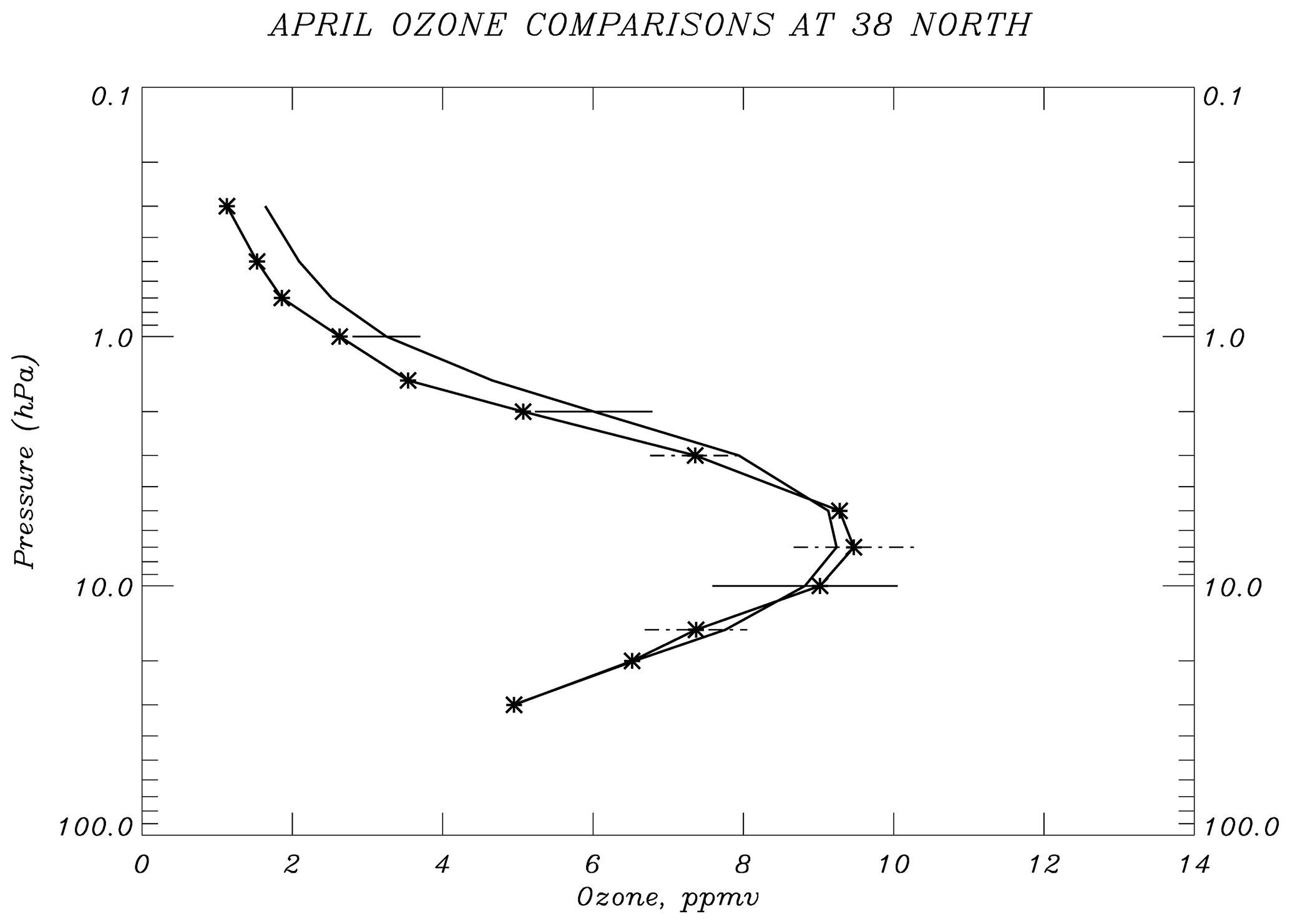
Figure 14LIMS V6 monthly zonal mean daytime ozone (solid) for April 1979 at 38∘ N compared with an average of three soundings (*) at Wallops Island, VA, 38∘ N, in April of 1976–1978. Horizontal bars are error estimates for LIMS (solid) and for a ROCOZ sounding (dashed).
Figure 15 shows V6 daytime minus ROCOZ average profiles at Wallops Island (38∘ N) for November, March, April, and May. The ozone differences are within their combined error estimates for the middle stratosphere but are larger in the upper stratosphere and especially the mesosphere. The increasingly positive V6 day minus ROCOZ differences in the lower mesosphere from winter to late spring are due to uncorrected NLTE effects for V6 from CO2 and ozone that increase toward lower solar zenith angles (Solomon et al., 1986; Mlynczak and Drayson, 1990). On the other hand, the V6 daytime ozone of April and May is also larger than ROCOZ ozone at 1.5 to 3 hPa, where NLTE should not be an issue (Edwards et al., 1996). While there may be excess V6 ozone due to a slight negative bias for V6 T(p) at those pressure altitudes, it may also be that the ROCOZ climatology at Wallops Islands is not truly representative of zonal average ozone for those months of 1979. In the next section, we report on time series of fields of potential vorticity, ozone, and H2O from their V6 level 3 combined (A+D) products for the middle stratosphere, where those parameters are not expected to have diurnal variations and should serve as tracers of atmospheric transport.
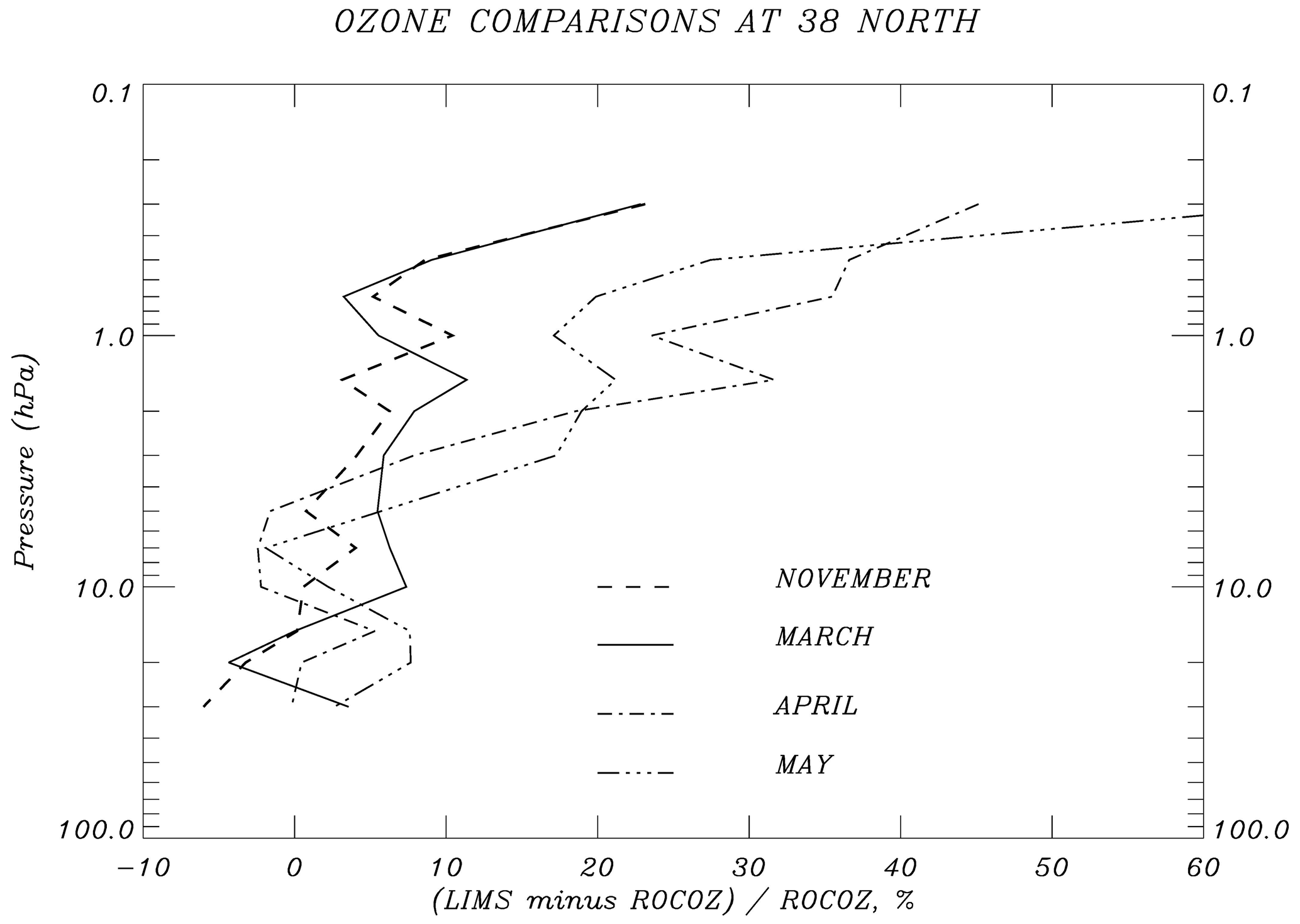
Figure 15Monthly zonal mean V6 daytime ozone minus ROCOZ ozone (in %) for 4 months at 38∘ N.
Dunkerton and DeLisi (1986) made use of LIMS V5 GPH and temperature data to calculate potential vorticity (PV) and then show how PV evolved in the NH on the 850 K potential temperature (∼10 hPa) surface during January and February 1979. Butchart and Remsberg (1986; hereafter, BR) also calculated PV from the V5 data and plotted its evolution during the winter of 1978–1979 in terms of the fractional area of the NH enclosed by the horizontal projection of a given PV contour on the 850 K surface. These so-called area diagnostic analyses of BR work well for a parameter like PV that is monotonic with latitude, having its highest value at the pole.
New time series analyses of PV from the combined V6 data are in Fig. 16, calculated from the level 3, daily six-wavenumber, zonal coefficients of GPH and temperature. Equivalent latitude (on the right ordinate) represents the latitude at which a zonally symmetric PV contour would lie if it enclosed the given fractional area shown on the left ordinate. PV data for Fig. 16 have a 7 d smoothing, and the NH fractional area extends only to 20∘ equivalent latitude because calculations of absolute vorticity are not as accurate near the Equator. The PV results for V6 are nearly identical to those for V5 in BR (their Fig. 4). Notably, the polar vortex (defined by highest PV values) erodes during winter and the adjacent “surf-zone”, having much lower PV gradients, expands in area due to the “breaking” of planetary waves and the associated meridional mixing of vortex and lower-latitude air.
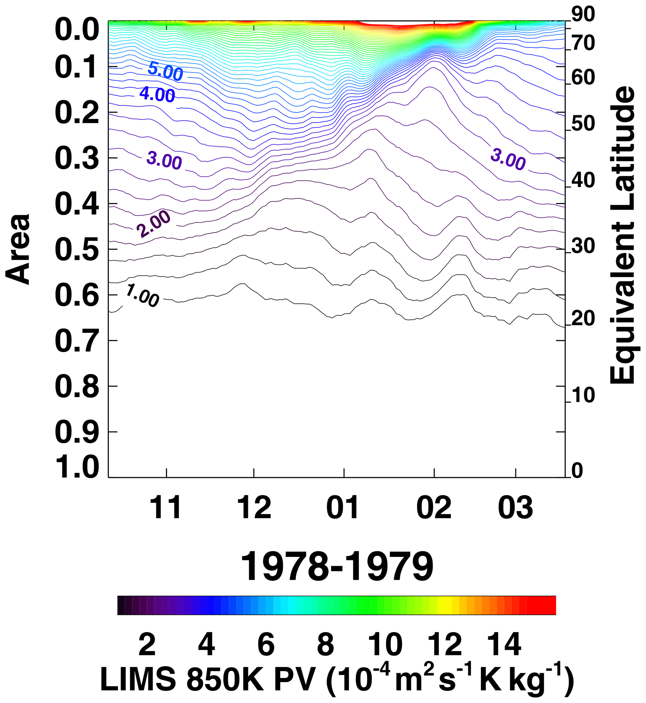
Figure 16Area diagnostic plot of time series of NH potential vorticity (PV) contours on the 850 K potential temperature surface for comparison with Butchart and Remsberg (1986, their Fig. 4). PV comes from LIMS V6 level 3 geopotential height and temperature data. Contour interval (CI) is 0.25 PV units (units of PV are 10−4 m2 s−1 K kg−1). Tick marks on the abscissa denote the 15th day of each month.
Ozone is an effective tracer of the transport of air in and around the winter polar vortex on the 850 K surface (∼10 hPa) (Leovy et al., 1985). Ozone also varies nearly monotonically at this level, but with highest values at low latitudes and lowest values near the pole. BR analyzed the evolution of V5 ozone (see their Fig. 10b). They compared its changes with those of PV and found good correspondence for the large-scale features of the two distributions. Fig. 17 is the new ozone time series at 850 K from the gridded V6 data, and it compares well with the calculations of BR from the V5 ozone. One significant change with V6 is that the ozone contours of 6.8 through 7.2 ppmv of early February indicate very weak gradients within the surf zone, as it expands following the major warming event of late January. There is also an associated, diabatic cross-isentropic transport of ozone within the surf zone during that time (e.g., Butchart, 1987). The improved continuity of the ozone time series from V6 is a result of the better spatial sampling for the radiances, of the retrievals of T(p) profiles, and of the corresponding changes for the registration of the ozone radiance profiles and retrieved ozone mixing ratios.
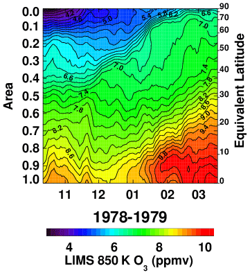
Figure 17Area diagnostic plot of V6 level 3 ozone for comparison with Fig. 16. Ozone contour interval is 0.2 ppmv. Tick marks on the abscissa indicate the 15th day of each month.
Water vapor is also a tracer of the net transport in the middle stratosphere. Figure 18 shows the corresponding time series of V6 H2O at 850 K. V6 H2O mixing ratio contours vary more smoothly than those from the V5 data in BR (their Fig. 12); the retrieved V6 H2O profiles are better resolved spatially and have better precision. There is good correspondence between H2O, PV, and ozone for the location and evolution of the edge of the polar winter vortex and for the expansion of the region of weak gradients at middle latitudes. Low values of H2O extend to the northern middle latitudes, and high values of H2O descend within the polar vortex from November through January, indicating an acceleration of the Brewer–Dobson circulation during that winter. There is also a modest expansion of weak H2O gradients between 40∘ N and 60∘ N equivalent latitude from mid-November to mid-December. This region coincides with the time of the Canadian warming and an exchange of air between polar and middle latitudes.

This study provides some insight into the quality of the LIMS V6 level 3 product and the generation of daily gridded species distributions on pressure surfaces. Monthly zonal mean distributions are available within the SPARC-DI database for comparisons with model simulations of middle-atmosphere species. We also provide the corresponding monthly zonal mean distributions of temperature for SPARC-DI and diagnostic evidence of effects of residual temperature biases in the V6 ozone, H2O, and HNO3 distributions. Those species exhibit ascending minus descending (A−D or day minus night at most latitudes) anomalies, especially in the middle and lower stratosphere. In particular, the A−D ozone and H2O values are larger than expected due to not accounting for all of the horizontal temperature structure, which affects forward radiance calculations through the Planck blackbody function, the retrievals of T(p), and the registration of species radiance profiles with pressure. It may be that the V6 species distributions within the SH have better accuracy from along its ascending (A) orbital segments, since the tangent view paths for its profiles are more nearly in a zonal direction and do not have significant T(p) gradients. Finally, we found no clear evidence of temperature bias in V6 NO2.
Remsberg et al. (2013) reported that an assimilation of SBUV ozone along with the V6 A and D level 2 ozone profiles provides ozone distributions that agree well with balloon-sonde ozone in the lower stratosphere. However, we do not recommend assimilation studies based on only the V6 ozone profiles because of their small but persistent A−D differences, particularly at the edge of and within the winter polar vortex. V6 H2O profiles present similar assimilation problems. Instead, we recommend that researchers make use of the average (A+D) V6 level 3 product and/or the SPARC-DI monthly, zonal average distributions for their science studies of stratospheric ozone and H2O, at least where NLTE effects are not an issue. As an example, Tegtmeier et al. (2013) compared the combined V6 monthly stratospheric ozone distributions with ones from other satellite-based limb sensors, and they found good agreement. Thereafter, Shepherd et al. (2014) integrated the SPARC-DI V6 monthly zonal mean ozone above the tropopause and subtracted it from observed total ozone as part of their assessment of long-term trends of tropospheric ozone from models for 1978 and onward.
Remsberg et al. (2007, their Fig. 8b) found that zonal average V6 ozone in the middle stratosphere is higher than SBUV ozone by 4 %, which is well within the combined systematic errors of both experimental datasets. Correlative ozone measurements for the middle to upper stratosphere are too few and too inaccurate in 1978 and 1979 to determine whether the V6 A or D ozone is more accurate. Thus, we considered V6 monthly profile data versus a monthly daytime ozone climatology of the late 1970s obtained with the rocket-borne UV-absorption (ROCOZ) technique at Wallops Island, VA. We found agreement within their respective errors, except for the uppermost stratosphere and the lower mesosphere. We also calculated time series of V6 level 3 ozone and H2O at 850 K and looked for consistency between their fields and those of PV. In general, we found good agreement with similar studies of BR (1986) based on V5 data. However, the time series from V6 shows better continuity during dynamically active periods.
The LIMS experience has been of benefit for the design of follow-on broadband, limb infrared measurements. One satellite experiment, the Sounding of the Atmosphere using Broadband Emission Radiometry (SABER), has been obtaining measurements of temperature, ozone, and H2O from 2002–2020 (e.g., Remsberg et al., 2008; Rong et al., 2009). Improvements from SABER compared to LIMS are (1) reductions in electronics and detector noise for its narrow-band and wide-band CO2 channels by factors of 5 and 16, respectively, and for its ozone channel by a factor of 20; (2) common 2 km IFOVs for its CO2 (for temperature) and species channels to account for diurnal temperature signals in the retrievals of ozone and H2O; (3) an ozone filter bandpass of about 1000 to 1150 cm−1 to avoid the NLTE emissions from the CO2 laser band at 960 cm−1; and (4) NLTE algorithms for retrievals of T(p), ozone, and H2O in the mesosphere. SABER instrument operation is stable and its orbital attitude information is accurate (Mlynczak et al., 2020). SABER tangent view paths are 90∘ away from the spacecraft velocity vector or in nearly a zonal direction for the low and middle latitudes, where zonal temperature gradients are weak. There is little need to correct for T(p) gradients in the SABER algorithms, except when viewing the high latitudes. Accordingly, diurnal temperature and ozone variations from SABER compare reasonably with those from microwave measurements and with model estimates (e.g., Huang et al., 2010a, b; Frith et al., 2020).
The LIMS V6 data archive is at the NASA EARTHDATA site of EOSDIS and its website: https://disc.gsfc.nasa.gov/datacollection/LIMSN7L2_006.html (Remsberg, 2008) and https://disc.gsfc.nasa.gov/datacollection/LIMSN7L3_006.html (Remsberg et al., 2011). The ROCOZ ozone climatology at Wallops Island is available at http://woudc.org/data/products/ (WOUDC, 2021) (also available from arjkrueger@gmail.com upon request). The SPARC-Data Initiative site is located at https://doi.org/10.5281/zenodo.4265393 (Hegglin et al., 2020). We acknowledge the individual instrument teams and respective space agencies for making their measurements available, and the Data Initiative of WCRP's (World Climate Research Programme) SPARC (Stratospheric Processes and their Role in Climate) project for organizing and coordinating the compilation of the chemical trace gas datasets used in this work.
The supplement related to this article is available online at: https://doi.org/10.5194/amt-14-2185-2021-supplement.
ER prepared most of the figures and wrote the manuscript with contributions from all co-authors. MN produced plots of the ascending minus descending radiances. VLH prepared the time series plots of PV, ozone, and H2O. AK provided his early rocketsonde data on ozone and temperature and their estimated errors.
The authors declare that they have no conflict of interest.
We are grateful to Krzysztof Wargan, who raised concerns about the assimilation of alternating V6 A and D polar ozone profiles during a re-analysis run of the MERRA model. We especially thank John Burton, Larry Gordley, Thomas Marshall, and Earl Thompson for producing the V6 level 2 dataset. Gretchen Lingenfelser generated the V6 level 3 zonal Fourier coefficient data. We thank John Gille and Ernest Hilsenrath, who read and commented on a draft version of the manuscript. V. Lynn Harvey acknowledges support from NSF CEDAR grant 1343031, NASA LWS grant NNX14AH54G, NASA HGI grant NNX17AB80G, and NASA HSR grant 80NSSC18K1046. Ellis Remsberg and Murali Natarajan carried out their work while serving as Distinguished Research Associates of the Science Directorate at NASA Langley.
This research has been supported by the Sciences Directorate (NASA Langley Research Center).
This paper was edited by Christian von Savigny and reviewed by two anonymous referees.
Barnett, J. and Corney, M.: Middle atmosphere reference model derived from satellite data, in: Handbook for Middle Atmosphere Program, edited by: Labitzke, K., Barnett, J. J., and Edwards, B., vol. 16, 47–137, NASA Contractor Report 176321, Document ID 19860003346, available at: https://ntrs.nasa.gov (last access 12 November 2019), 1985.
Brasseur, G. and Solomon, S.: Aeronomy of the Middle Atmosphere: Chemistry and Physics of the Stratosphere and Mesosphere, 3rd Edn., Springer, Dordrecht, the Netherlands, 644 pp., 2005.
Butchart, N.: Evidence for planetary wave breaking from satellite data: the relative roles of diabatic effects and irreversible mixing, in: Transport Processes in the Middle Atmosphere, edited by: Visconti, G. and Garcia, R., D. Reidel Publishing Co., Dordrecht, Holland, 121–136, 1987.
Butchart, N. and Remsberg, E. E.: The area of the stratospheric polar vortex as a diagnostic for tracer transport on an isentropic surface, J. Atmos. Sci., 43, 1319–1339, https://doi.org/10.1175/1520-0469(1986)043<1319:TAOTSP>2.0.CO;2, 1986.
Dunkerton, T. J. and DeLisi, D. P.: Evolution of potential vorticity in the winter stratosphere of January–February 1979, J. Geophys. Res. 91, 1199–1208, https://doi.org/10.1029/JD091iD01p01199, 1986.
Edwards, D. P., Kumer, J. B., Lopez-Puertas, M., Mlynczak, M. G., Gopalan, A., Gille, J. C., and Roche, A.: Non-local thermodynamic equilibrium limb radiance near 10 µm as measured by UARS CLAES, J. Geophys. Res., 101, 26577–26588, https://doi.org/10.1029/96JD02133, 1996.
Finger, F. G., Gelman, M. E., Schmidlin, F. J., Leviton, R., and Kennedy, V. W.: Compatibility of meteorological rocketsonde data as indicated by international comparisons tests, J. Atmos. Sci., 32, 1705–1714, https://doi.org/10.1175/1520-0469(1975)032<1705:COMRDA>2.0.CO;2, 1975.
Frith, S. M., Bhartia, P. K., Oman, L. D., Kramarova, N. A., McPeters, R. D., and Labow, G. J.: Model-based climatology of diurnal variability in stratospheric ozone as a data analysis tool, Atmos. Meas. Tech., 13, 2733–2749, https://doi.org/10.5194/amt-13-2733-2020, 2020.
Gille, J. C. and Russell III, J. M.: The limb infrared monitor of the stratosphere: experiment description, performance, and results, J. Geophys. Res., 84, 5125–5140, https://doi.org/10.1029/JD089iD04p05125, 1984.
Gille, J. C., Russell III, J. M., Bailey, P. L., Gordley, L. L., Remsberg, E. E., Lienesch, J. H., Planet, W. G., House, F. B., Lyjak, L. V., and Beck, S. A.: Validation of temperature retrievals obtained by the limb infrared monitor of the stratosphere (LIMS) experiment on NIMBUS 7, J. Geophys. Res., 89, 5147–5160, https://doi.org/10.1029/JD089iD04p05147, 1984.
Gordley, L. L. and Russell, J. M.: Rapid inversion of limb radiance data using an emissivity growth approximation, Appl. Opt., 20, 807–813, https://doi.org/10.1364/AO.20.000807, 1981.
Haigh, J. D. and Pyle, J. A.: Ozone perturbation experiments in a two-dimensional circulation model, Q. J. Roy. Meteorol. Soc., 108, 551–574, https://doi.org/10.1002/qj.49710845705, 1982.
Hegglin, M. I., Tegtmeier, S., Anderson, J., Bourassa, A. E., Brohede, S., Degenstein, D., Froidevaux, L., Funke, B., Gille, J., Kasai, Y., Kyrölä, E., Lumpe, J., Murtagh, D., Neu, J. L., Pérot, K., Remsberg, E., Rozanov, A., Toohey, M., von Clarmann, T., Walker, K. A., Wang, H. J., Damadeo, R., Fuller, R., Lingenfelser, G., Roth, C., Ryan, N. J., Sioris, C., Smith, L., and Weigel, K.: SPARC Data Initiative monthly zonal mean composition measurements from stratospheric limb sounders (1978–2018), (Version p01) [Data set], Earth System Science Data (ESSD), Zenodo, https://doi.org/10.5281/zenodo.4265393, 2020.
Hitchman, M. H., and Leovy, C. B.: Diurnal tide in the equatorial middle atmosphere as seen in LIMS temperatures, J. Atmos. Sci., 42, 557–561, https://doi.org/10.1175/1520-0469(1985)042<0557:DTITEM>2.0.CO;2, 1985.
Huang, F. T., McPeters, R. D., Bhartia, P. K., Mayr, H. G., Frith, S. M., Russell III, J. M., and Mlynczak, M. G.: Temperature diurnal variations (migrating tides) in the stratosphere and lower mesosphere based on measurements from SABER on TIMED, J. Geophys. Res., 115, D16121, https://https://doi.org/10.1029/2009JD013698, 2010a.
Huang, F. T., Mayr, H. G., Russell III, J. M., and Mlynczak, M. G.: Ozone diurnal variations in the stratosphere and mesosphere, based on measurements from SABER on TIMED, J. Geophys. Res., 115, D24308, https://https://doi.org/10.1029/2010JD014484, 2010b.
Kiefer, M., Arnone, E., Dudhia, A., Carlotti, M., Castelli, E., von Clarmann, T., Dinelli, B. M., Kleinert, A., Linden, A., Milz, M., Papandrea, E., and Stiller, G.: Impact of temperature field inhomogeneities on the retrieval of atmospheric species from MIPAS IR limb emission spectra, Atmos. Meas. Tech., 3, 1487–1507, https://doi.org/10.5194/amt-3-1487-2010, 2010.
Krueger, A. J.: The mean ozone distribution from several series of rocket soundings to 52 km at latitudes from 58∘ S to 64∘ N, Journal of Pure and Applied Geophysics, 106, 1272–1280, https://doi.org/10.1007/BF00881079, 1973.
Krueger, A. J: Inference of photochemical trace gas variations from direct measurements of ozone in the middle atmosphere, PhD thesis, Colorado State Univ., Fort Collins, CO, 1984.
Krueger, A. J. and Minzner, R. A.: A mid-latitude ozone model for the 1976 U. S. standard atmosphere, J. Geophys. Res., 81, 4477–4481, https://doi.org/10.1029/JC081i024p04477, 1976.
Leovy, C. B., Sun, C-R., Hitchman, M. H., Remsberg, E. E., Russell, III, J. M., Gordley, L. L., Gille, J. C., and Lyjak, L. V.: Transport of ozone in the middle stratosphere: evidence for planetary wave breaking, J. Atmos. Sci., 42, 230–244, https://doi.org/10.1175/1520-0469(1985)042<0230:TOOITM>2.0.CO;2, 1985.
London, J., Frederick, J. E., and Anderson, G. P.: Satellite observations of the global distribution of stratospheric ozone, J. Geophys. Res., 82, 2543–2556, https://doi.org/10.1029/JC082i018p02543, 1977.
Lopez-Puertas, M. and Taylor, F. W.: Non-LTE Radiative transfer in the Atmosphere, World Scientific Publ. Co., River Edge, NJ, USA, 504 pp., 2001.
Manuilova, R. O., Gusev, O. A., Kutepov, A. A., von Clarmann, T., Oelhaf, H., Stiller, G. P, Wegner, A., Lopez-Puertas, M., Martin-Torres, F. J., Zaragoza, G., and Flaud, J.-M.: Modelling of non-LTE limb spectra of i.r. ozone bands for the MIPAS space experiment, J. Quant. Spectrosc. Ra., 59, 405–422, https://doi.org/10.1016/S0022-4073(97)00120-9, 1998.
Mertens, C. J., Mlynczak, M. G., Lopez-Puertas, M., and Remsberg, E. E.: Impact of non-LTE processes on middle atmospheric water vapor retrievals from simulated measurements of 6.8 µm Earth limb emission, Geophys. Res. Lett., 29, 2-1–2-4, https://doi.org/10.1029/2001GL014590, 2002.
Mlynczak, M. G. and Drayson, R.: Calculation of infrared limb emission by ozone in the terrestrial middle atmosphere 2. Emission calculations, J. Geophys. Res., 95, 16513–16521, https://doi.org/10.1029/JD095iD10p16513, 1990.
Mlynczak, M. G., Daniels, T., Hunt, L. A., Yue, J., Marshall, B. T., Russell, J. M., III, Remsberg, E. E., Tansock, J., Esplin, R., Jensen, M., Shumway, A., Gordley, L., and Yee, J.-H.: Radiometric stability of the SABER instrument, Earth Space Sci., 7, e2019EA001011, https://doi.org/10.1029/2019EA001011, 2020.
Remsberg, E.: LIMS/Nimbus-7 Level 2 Vertical Profiles of O3, NO2, H2O, HNO3, Geopotential Height, and Temperature V006, Version: 006, Goddard Earth Sciences Data and Information Services Center, available at: https://disc.gsfc.nasa.gov/datacollection/LIMSN7L2_006.html (last access: 11 March 2021), 2008.
Remsberg, E. and Lingenfelser, G.: LIMS Version 6 Level 3 dataset, NASA-TM-2010-216690, available at: http://www.sti.nasa.gov (last access: 17 September 2019), 13 pp., 2010.
Remsberg, E., Lingenfelser, G., Natarajan, M., Gordley, L., Marshall, B. T., and Thompson, E.: On the quality of the Nimbus 7 LIMS version 6 ozone for studies of the middle atmosphere, J. Quant. Spectros. Ra., 105, 492–518, https://doi.org/10.1016/j.jqsrt.2006.12.005, 2007.
Remsberg, E., Natarajan, M., Marshall, B. T., Gordley, L. L., Thompson, R. E., and Lingenfelser, G.: Improvements in the profiles and distributions of nitric acid and nitrogen dioxide with the LIMS version 6 dataset, Atmos. Chem. Phys., 10, 4741–4756, https://doi.org/10.5194/acp-10-4741-2010, 2010.
Remsberg, E., et al.: LIMS/Nimbus-7 Level 3 Daily 2 deg Latitude Zonal Fourier Coefficients of O3, NO2, H2O, HNO3, Geopotential Height, and Temperature V006, Version: 006, Goddard Earth Sciences Data and Information Services Center (GES DISC), available at: https://disc.gsfc.nasa.gov/datacollection/LIMSN7L3_006.html (last access: 11 March 2021), 2011.
Remsberg, E., Natarajan, M., Fairlie, T. D., Wargan, K., Pawson, S., Coy, L., Lingenfelser, G., and Kim, G.: On the inclusion of Limb Infrared Monitor of the Stratosphere version 6 ozone in a data assimilation system, J. Geophys. Res., 118, 7982–8000, https://doi.org/10.1002/jgrd.50566, 2013.
Remsberg, E. E., Russell III, J. M., Gille, J. C., Bailey, P. L., Gordley, L. L., Planet, W. G., and Harries, J. E.: The validation of Nimbus 7 LIMS measurements of ozone, J. Geophys. Res., 89, 5161–5178, https://doi.org/10.1029/JD089iD04p05161, 1984.
Remsberg, E. E., Haggard, K. V., and Russell III, J. M.,: Estimation of Synoptic Fields of Middle Atmosphere Parameters from Nimbus-7 LIMS Profile Data, J. Atmos. Ocean. Technol., 7, 689–705, 1990.
Remsberg, E. E., Gordley, L. L, Marshall, B. T., Thompson, R. E., Burton, J., Bhatt, P., Harvey, V. L., Lingenfelser, G., and Natarajan, M.: The Nimbus 7 LIMS version 6 radiance conditioning and temperature retrieval methods and results, J. Quant. Spectros. Ra., 86, 395–424, https://doi.org/10.1016/j.jqsrt.2003.12.007, 2004.
Remsberg, E. E., Marshall, B. T., Garcia-Comas, M., Krueger, D., Lingenfelser, G. S., Martin-Torres, J., Mlynczak, M. G., Russell III, J. M., Smith, A. K., Zhao, Y., Brown, C., Gordley, L. L., Lopez-Gonzalez, M. J., Lopez-Puertas, M., She, C. Y., Taylor, M. J., and Thompson, E.: Assessment of the quality of the Version 1.07 temperature versus pressure profiles of the middle atmosphere from TIMED/SABER, J. Geophys. Res., 113, D17101, https://doi.org/10.1029/2008JD010013, 2008.
Remsberg, E. E., Natarajan, M., Lingenfelser, G. S., Thompson, R. E., Marshall, B. T., and Gordley, L. L.: On the quality of the Nimbus 7 LIMS Version 6 water vapor profiles and distributions, Atmos. Chem. Phys., 9, 9155–9167, https://doi.org/10.5194/acp-9-9155-2009, 2009.
Roewe, D. A., Gille, J. C., and Bailey, P. L.: Infrared limb scanning in the presence of horizontal temperature gradients: an operational approach, Appl. Opt., 21, 3775–3783, https://doi.org/10.1364/AO.21.003775, 1982.
Rong, P. P., Russell III, J. M., Mlynczak, M. G., Remsberg, E. E., Marshall, B. T., Gordley, L. L., and Lopez-Puertas, M.: Validation of Thermosphere Ionosphere Mesosphere Energetics and Dynamics/Sounding of the Atmosphere using Broadband Emission Radiometry (TIMED/SABER) v1.07 ozone at 9.6 µm in altitude range 15–70 km, J. Geophys. Res., 114, D04306, https://doi.org/10.1029/2008JD010073, 2009.
Russell III, J. M., Gille, J. C., Remsberg, E. E., Gordley, L. L., Bailey, P. L., Drayson, S. R., Fischer, H., Girard, A., Harries, J. E., and Evans, W. F. J.: Validation of nitrogen dioxide results measured by the Limb Infrared Monitor of the Stratosphere (LIMS) experiment on Nimbus 7, J. Geophys. Res., 89, 5099–5107, https://doi.org/10.1029/JD089iD04p05099, 1984.
Sakazaki, T., Fujiwara, M., Mitsuda, C., Imai, K., Manago, N., Naito, Y., Nakamura, T., Akiyoshi, H., Kinnison, D., Sano, T., Suzuki, M., and Shiotani, M.: Diurnal ozone variations in the stratosphere revealed in observations from the Superconducting Submillimeter-Wave Limb-Emission Sounder (SMILES) on board the International Space Station (ISS), J. Geophys. Res., 118, 2991–3006, https://doi.org/10.1002/jgrd.50220, 2013.
Shepherd, T. G., Plummer, D. A., Scinocca, J. F., Hegglin, M. I., Fioletov, V. E., Reader, M. C., Remsberg, E., von Clarmann, T., and Wang, H. J.: Reconciliation of halogen-induced ozone loss with the total-column record, Nat. Geosci., 7, 443–449, https://doi.org/10.1038/ngeo2155, 2014.
Solomon, S., Kiehl, J. T., Kerridge, B. J., Remsberg, E. E., and Russell III, J. M.: Evidence for nonlocal thermodynamic equilibrium in the ν3 mode of mesospheric ozone, J. Geophys. Res., 91, 9865–9876, https://doi.org/10.1029/JD091iD09p09865, 1986.
Stratosphere-troposphere Processes and their Role in Climate (SPARC): The SPARC Data Initiative: Assessment of stratospheric trace gas and aerosol climatologies from satellite limb sounders, edited by: Hegglin, M. I. and Tegtmeier, S., , SPARC Report No. 8, WCRP-5/2017, available at: http://www.sparc-climate.org/publications/sparc-reports/ (last access: 12 March 2021), 2017.
Sun, C.-R. and Leovy, C.: Ozone variability in the equatorial middle atmosphere, J. Geophys. Res., 95, 13829–13849, https://doi.org/10.1029/JD095iD09p13829, 1990.
Tegtmeier, S., Hegglin, M. I., Anderson, J., Bourassa, A., Brohede, S., Degenstein, D., Froidevaux, L., Fuller, R., Funke, B., Gille, J., Jones, A., Kasai, Y., Krüger, K., Kyrölä, E., Lingenfelser, G., Lumpe, J., Nardi, B., Neu, J., Pendlebury, D., Remsberg, E., Rozanov, A., Smith, L., Toohey, M., Urban, J., von Clarmann, T., Walker, K. A., and Wang, R. H. H.: SPARC Data Initiative: A comparison of ozone climatologies from international satellite limb sounders, J. Geophys. Res., 118, 12229–12247, https://doi.org/10.1002/2013JD019877, 2013.
World Ozone and Ultraviolet Radiation Data Centre (WOUDC): Rocketsonde ozone data, Meteorological Service of Canada, available at: http://woudc.org/data/products/, last access: 12 March 2021.
- Abstract
- Introduction and objectives
- Characteristics of the V6 level 3 ozone, temperature, and water vapor
- Measurement, retrieval, and day–night differences for temperature
- Day–night differences in V6 species
- Ozone comparisons with rocket-borne measurements
- Seasonal transport of V6 ozone and water vapor
- Summary and recommendations
- Data availability
- Author contributions
- Competing interests
- Acknowledgements
- Financial support
- Review statement
- References
- Supplement