the Creative Commons Attribution 4.0 License.
the Creative Commons Attribution 4.0 License.
 | 22 Mar 2021
Relative sky radiance from multi-exposure all-sky camera images
Juan C. Antuña-Sánchez
Roberto Román
Victoria E. Cachorro
Carlos Toledano
César López
Ramiro González
David Mateos
Abel Calle
Ángel M. de Frutos
All-sky cameras are frequently used to detect cloud cover; however, this work explores the use of these instruments for the more complex purpose of extracting relative sky radiances. An all-sky camera (SONA202-NF model) with three colour filters narrower than usual for this kind of cameras is configured to capture raw images at seven exposure times. A detailed camera characterization of the black level, readout noise, hot pixels and linear response is carried out. A methodology is proposed to obtain a linear high dynamic range (HDR) image and its uncertainty, which represents the relative sky radiance (in arbitrary units) maps at three effective wavelengths. The relative sky radiances are extracted from these maps and normalized by dividing every radiance of one channel by the sum of all radiances at this channel. Then, the normalized radiances are compared with the sky radiance measured at different sky points by a sun and sky photometer belonging to the Aerosol Robotic Network (AERONET). The camera radiances correlate with photometer ones except for scattering angles below 10∘, which is probably due to some light reflections on the fisheye lens and camera dome. Camera and photometer wavelengths are not coincident; hence, camera radiances are also compared with sky radiances simulated by a radiative transfer model at the same camera effective wavelengths. This comparison reveals an uncertainty on the normalized camera radiances of about 3.3 %, 4.3 % and 5.3 % for 467, 536 and 605 nm, respectively, if specific quality criteria are applied.
- Article
(15376 KB) - Full-text XML
- Companion paper
-
Supplement
(1390 KB) - BibTeX
- EndNote


The knowledge of sky radiance is a fundamental problem of the radiative transfer in the atmosphere or other media where absorption, emission and scattering processes occur (Coulson, 1988). Restricted to the case of solar radiation in the atmosphere–surface of Earth, sky radiance depends on the Sun's position in the sky, and its angular distribution is mainly controlled by the light scattering caused by atmospheric gases through Rayleigh scattering (responsible for the colour of the blue sky under clear conditions) but also caused by aerosols and clouds through Mie scattering. The knowledge of the sky radiance is useful, among other fields, in photovoltaic production to calculate what solar radiation reaches an oriented panel (Li and Lam, 2007) and in human health to know the solar UV radiation dose received by a human body (Seckmeyer et al., 2013; Schrempf et al., 2017).
The spectral sky radiance reaching Earth's surface under cloud-free conditions is basically the solar irradiance scattered by gases and aerosols; therefore, the knowledge of the spectral sky radiance at different angles is a footprint of the aerosol properties; it implies that the sky radiance contains useful information that can be used for the retrieval of aerosol optical and microphysical properties (Nakajima et al., 1996; Dubovik and King, 2000). In fact, even relative sky radiance measurements (in arbitrary units) are useful for this purpose (Román et al, 2017a). Most remote sensing techniques, mainly those used by satellite platforms, are also based on upward sky radiance measurements formed by the radiation reflected by Earth's surface and scattered by the atmosphere, allowing us to determine the different atmospheric compounds.
Accurate measurements of the sky radiance are usually taken by photometers. As an example, the CE318 sun and sky photometer (Cimel Electronique S.A.S.), which is the reference instrument of the Aerosol Robotic Network (AERONET; https://aeronet.gsfc.nasa.gov, 8 March 2021), measures the absolute sky radiance at different geometries and wavelengths with an uncertainty of about 5 % (Holben et al., 1998). These sky radiance scans provide useful and accurate information (e.g. AERONET uses them to retrieve and provide aerosol products); however, the recorded sky radiances are only measured at some sky angular positions, and the more points that are measured, the more time is spent. It causes a temporal shift between measurements, and the sky scene can change during this time.
All-sky cameras are devices designed to capture images of the full hemispherical sky and consist usually of a charge-coupled device (CCD) or a complementary metal oxide semiconductor (CMOS) sensor looking at a mirror or with a mounted fisheye lens. The most frequent use of all-sky cameras is cloud cover detection (e.g. Tapakis and Charalambides, 2013, and references therein), but they have also been used for more complex purposes like solar irradiance forecasting (Alonso-Montesinos et al., 2015; Barbieri et al., 2017), to derive sky radiance and luminance measurements (Román et al., 2012; Tohsing et al., 2013), to retrieve aerosol properties (Cazorla et al., 2008; Román et al., 2017a), and to monitor aurora and airglow (Sigernes et al., 2014), among others. All-sky cameras are in general less accurate than well-calibrated photometers, but they are capable of obtaining a full map of the hemispherical sky radiance in a short time (a few seconds or less). In addition, the camera sensors allow for the variation in exposure time and gain, achieving a high dynamic range. These facts and the mentioned versatility of the all-sky cameras lead us to consider these devices as a complementary instrument of sun and sky photometers and as a cheaper alternative to perform sky radiance measurements in locations where photometers are not available.
This framework motivates the main objectives of this paper: to characterize the main properties of an all-sky camera and to develop a methodology to obtain relative sky radiances from this camera. This work also aims at quantifying the uncertainty of the sky radiances obtained by the proposed methodology through a direct comparison with photometer measurements, as well as with simulated radiances. The novelty of this work with respect to other works that also retrieve the sky radiance with sky cameras, such as Román et al. (2012), lies among other issues in the use of raw and multi-exposure images captured with narrower spectral filters.
This paper is structured as follows. Section 2 introduces the experimental site and the instrumentation. Section 3 describes in detail the methodology that has been developed to retrieve the relative sky radiances with the camera, while Sect. 4 presents the comparison of camera radiances with photometer measurements and simulated radiances. Finally, the main conclusions are summarized in Sect. 5.
All the measurements used in this work were carried out in a platform located on the rooftop of the science faculty of Valladolid, Spain (41.6636∘ N, 4.7058∘ W; 705 m above sea level). Valladolid, situated in the north-central Iberian Peninsula (150 km north of Madrid), is an urban city with a population of around 300 000 inhabitants (∼400 000 including the metropolitan area). The city is surrounded by rural areas, and it has a Mediterranean climate (Csb Köppen classification) with hot summers and cold winters. The predominant aerosol at Valladolid is classified as “clean continental” (Bennouna et al., 2013, Román et al., 2014), but occasionally Saharan dust particles are transported to Valladolid, especially in summer (Cachorro et al., 2016).
The instrumentation at the mentioned platform is managed by the “Grupo de Óptica Atmosférica” (Group of Atmospheric Optics) of the University of Valladolid (GOA-UVa). The GOA-UVa is in charge of the calibration of part of the AERONET photometers; hence, two reference photometers – accurately calibrated by the Langley plot at the high-altitude station Izaña (Toledano et al., 2018) – and various field photometers under calibration are always in operation at the platform. All the photometers are different versions of the CE318 (Cimel Electronique S.A.S.). The most recent model is the CE318-T sun, sky and moon photometer which allows for measurements of direct solar and lunar irradiance to derive the aerosol optical depth (AOD) at several wavelengths. This photometer (and older versions) is also capable of taking measurements of sky radiance at various wavelengths. The CE318-T mainly makes sky radiance scans at two different configurations: almucantar (zenith angle is equal to solar zenith angle, SZA, while the azimuth angle varies) and hybrid (a mix between almucantar and principal plane) scans (Sinyuk et al., 2020). Both configurations present spatial symmetry regarding the Sun's position, which is useful to reject cloud-contaminated measurements comparing left and right observations. CE318-T usually is configured to measure sky radiances at 380, 440, 500, 675, 870, 1020 and 1640 nm thanks to narrow interference filters mounted in a filter wheel. The multi-wavelength sky radiance measurements are used by AERONET to retrieve aerosol properties by inversion techniques (Dubovik et al., 2000; Sinyuk et al., 2020) like aerosol size distribution, complex refractive indices and the fraction of spherical particles (sphericity factor).
This work uses the photometer sky radiances at 440, 500 and 675 nm measured at Valladolid for both AERONET almucantar (only for ) and hybrid scenarios. These data have been directly obtained from the AERONET website (Aerosol inversions v3 – Download Tool), version 3 level 1.5 data. The size distribution, refractive indices and sphericity factor products of AERONET version 3 level 1.5 data (Sinyuk et al., 2020) have been also downloaded for this work.
The mentioned GOA-UVa platform is also equipped with a SONA202-NF (Sieltec Canarias S.L.) all-sky camera. This device is a prototype that mainly consists of a CMOS coupled with a fisheye lens, both encapsulated in a weatherproof case with a transparent glass dome. The camera is horizontally levelled to receive the sky radiance of the full hemispherical sky. The CMOS sensor is the SONY IMX249 and is configured to save raw images of 1172×1158 pixels with a resolution of 10 bits. This sensor has a Bayer filter mosaic following an RGGB pattern: half of the pixels are mainly sensitive to green (G), a fourth of them to red (R), and the other fourth to blue (B). The spectral response of these filters, obtained from the data sheet from the CMOS manufacturer, is shown in Fig. 1a. An additional RGB tri-band filter (Fig. 1b; spectral response provided by the manufacturer) is over the full mosaic in the SONA202-NF in order to reduce the width of the colour filters. As a result, Fig. 1c shows the final spectral response of the red, green and blue pixels which is narrower than without the tri-band filter; this additional filter also reduces (but does not fully eliminate) the overlapping between the colour channels.
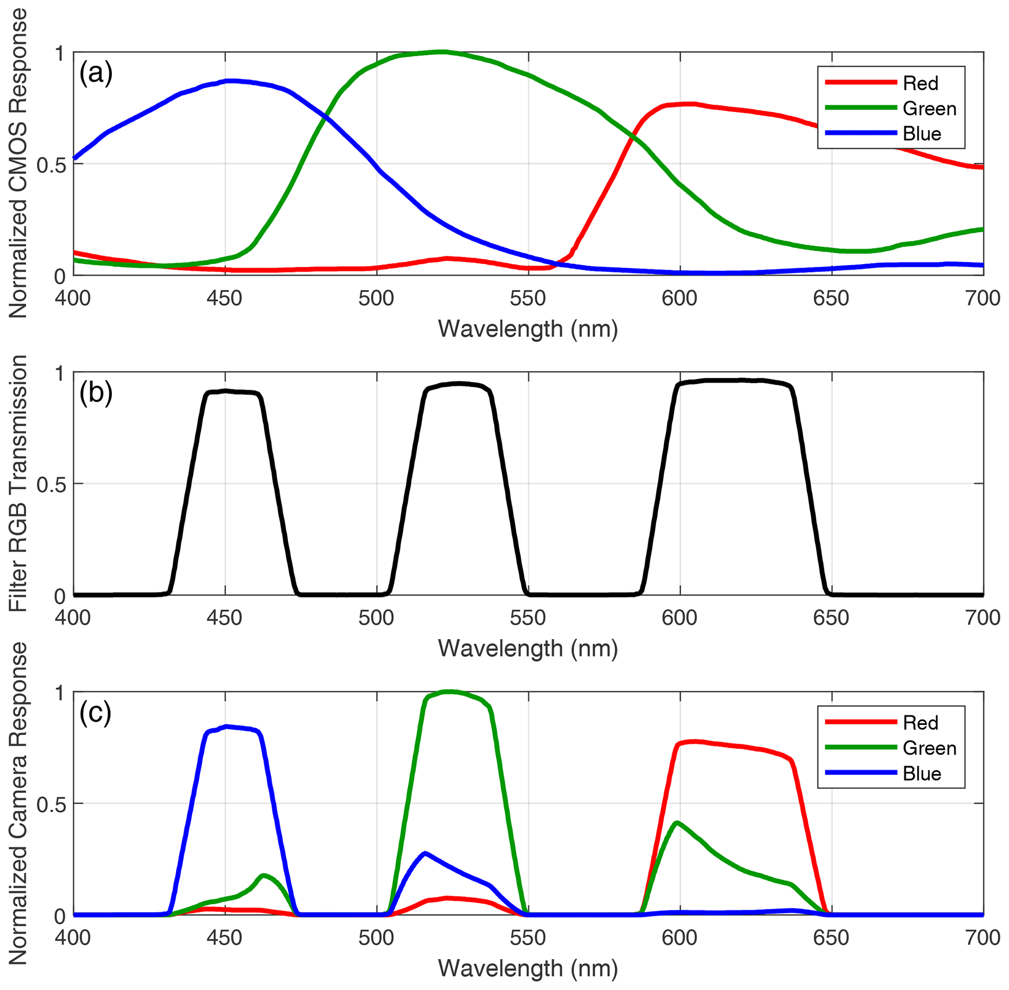
Figure 1Spectral response of (a) CMOS sensor Bayer filters, (b) RGB tri-band filter and (c) the all-sky camera (both filters together).
The sensor allows us to take pictures at different time exposures and signal amplifications (ISO). This all-sky camera is configured to take a set of raw images every 5 min with different exposure times in order to have enough pixel signal without saturation in the brightest (lower exposure times) and in the darkest (higher exposure times) sky parts. Two different exposure configurations are set in the camera: daytime and night-time due to the need for different exposure times, but this paper is only focused on daytime mode which was assumed for all images with SZAs below 95∘. No amplification is used in daytime mode. The exposure times used for each set of multi-exposure raw images are t1=0.3 µs, t2=0.4 µs, t3=0.6 µs, t4=1.2 µs, t5=2.4 µs, t6=4.8 µs and t7=9.6 µs. These exact exposure values are entered in the camera software; however, some tests varying these values indicated that the real exposure times could be discretized, showing equal images for different but close exposure times. Conversely, other images showed significant jumps in the recorded signal from images with small differences in the introduced exposure times.
The time expended to take the seven daytime raw images is a few seconds, and, after they are recorded, all images are saved together with additional metadata (such as sensor temperature) in one *.h5 file to reduce memory. Finally, the camera has been geometrically calibrated using a set of cloud-free night-time images from the ORION software (Antuña-Sánchez et al., 202), which determines the position of the sky (azimuth and zenith) viewed by each pixel and its field of view (FOV) through the star positions in the images.
3.1 Effective wavelengths
The three camera channels are sensitive to a broadband range of wavelengths because of the width of their spectral response (as discussed above; see Fig. 1). However, the measured broadband radiance can be assigned to an effective wavelength assuming the recorded broadband signal is proportional to the radiance at this effective wavelength (Román et al., 2017a). The ratio of two broadband measurements which are taken under different conditions but with the same instrument (the same spectral response) is equal to the ratio of the same measurements taken with an instrument which is only sensitive at the effective wavelength (Kholopov, 1975). The effective wavelength of each channel can be calculated by the convolution of the measured radiance by the channel spectral response, as was explained by Román et al. (2017a).
The effective wavelength of each channel has been calculated in this work for 200 different sky scenarios following the same method as in Román et al. (2012). To this end, the spectral diffuse sky radiance has been simulated using the libRadtran 1.7 radiative transfer package (Mayer and Kylling, 2005) for SZA values from 10 to 80∘ (in 10∘ steps), Angström exponent values from 0.2 to 1.8 (in 0.4 steps) and turbidity coefficient values (AOD at 1000 nm) from 0.01 to 0.21 (in 0.05 steps). Each simulation has been used to obtain an effective wavelength at each channel given a total of 200 different effective wavelengths per channel. The median (± standard deviation) of all obtained effective wavelengths is 605±3 nm, 536±3 nm and 467±2 nm for the red, green and blue channels, respectively. These obtained values have been assumed to be the effective wavelengths of the analysed camera. These results are similar to those obtained by Román et al. (2012), especially at G and B channels, for their all-sky camera model with a wider spectral response.
3.2 White balance
The channel spectral response affects the final colour image after a demosaicing (interpolation of the pixel signals of a channel to the pixels of the other channels) of the raw recorded image. Hence, a white balance is frequently used to obtain a final true colour demosaiced image. White balance mainly consists of multiplication of the recorded signal at each channel by a scaling factor (white balance scaling factor, WBSF) which is different for each R, G and B channel; it weights the relationship between the three colour channels, achieving a realistic final colour. The SONA202-NF used in this work was configured to provide a raw image with a previous white balance applied, in which the G and B channels are multiplied by ∼1.1 and 2.1, respectively, while the R channel remains the same (multiplied by 1).
This fact makes the direct demosaiced image of the analysed camera look more realistic. It can be observed in the example pictures of Fig. 2, in which Fig. 2a shows a direct image with applied white balance showing a more realistic blue sky colour than Fig. 2b, in which the same picture is shown but with G and B channels divided by their white balance scaling factors. This image presents a more greenish and less bluish sky. A true colour image is useful for the all-sky camera primary objective of detecting clouds. However, the application of the white balance scaling factors before obtaining the raw image reduces the image dynamic range since it can saturate pixel signals which initially were not saturated, especially at the blue channel in this case because the signal is multiplied by the mentioned factor of 2.1.
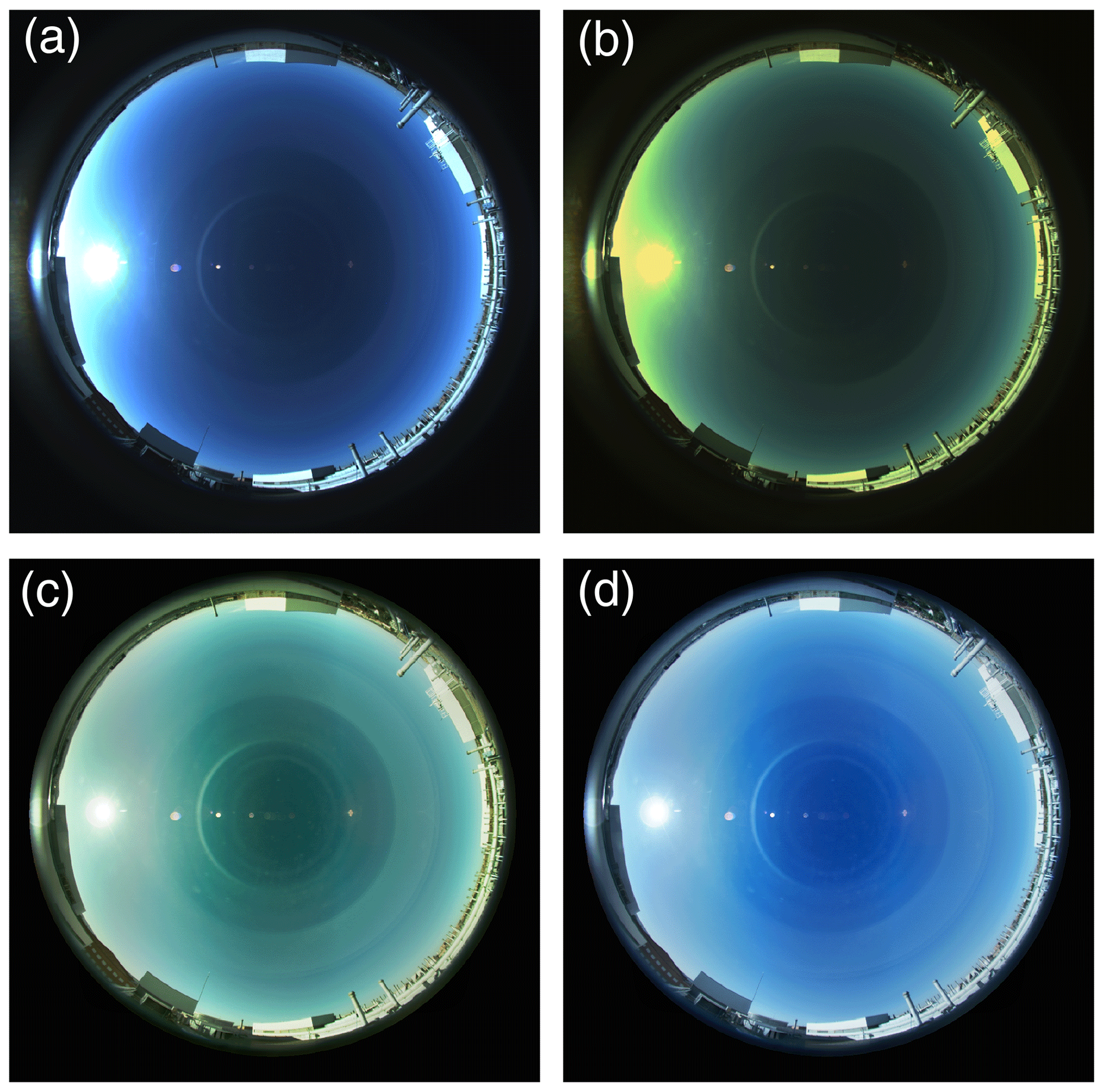
Figure 2Colour sky images of Valladolid on 17 August 2019 at 07:25 UTC of the (a) direct capture with exposure time equal to t4, (b) direct capture with exposure time equal to t4 but removing the previous white balance, (c) tone map of HDR image and (d) tone map of HDR image but with white balance applied.
3.3 Dark signal and hot pixels
The recorded signal of each pixel depends on the received light (photons converted to electrons), but some pixel signal appears in the recorded images even in the absence of light. This signal without light is called readout noise, and it is caused by camera electronics (amplification, analogue to digital conversion, etc.) in the readout process. The readout noise is Gaussian distributed; hence, the cameras usually add an offset (black level) to the recorded raw values in order to detect also negative readout noise values (signal below the offset). Summarizing, the recorded signal in one pixel is the signal generated by the number of absorbed photons plus the black level signal (offset) plus the total noise (being the readout noise part of the total noise).
The analysed camera was covered for 2.5 d with a metal piece designed to block all the incoming sky light. Meanwhile, the camera was capturing multi-exposure images as in its operational routine. A total of 413 images (dark frames) per exposure time were acquired in daytime mode. The red channel of all these dark frames has been used to determine the black level since this channel is the only one not affected by the mentioned white balance process. The mode and median of all red pixels are 30 digital counts (unit: DC) for each one of the 2891 (413 dark frames × 7 exposures) measured dark frames at the different time exposures; this reveals the black level of the sensor is 30 DC. Hence, the signal at the R, G and B channels has been corrected for black level offset and white balance by the next equation:
where Rc, Gc and Bc are the black level and white balance corrected signal of R, G and B channels, respectively, Rraw, Graw and Braw are the recorded raw camera signals, and WBSFR, WBSFG and WBSFB are the white balance scaling factors of the R (WBSFR=1), G (WBSFG=1.1) and B (WBSFB=2.1) channels, respectively. After this correction, the readout noise must be the same for the three channels.
All the dark frames have been corrected by Eq. (1), and the mean (MDFS, mean dark frame signal) and standard deviation (σDFS) of the signal of all pixels (including the three channels) have been calculated for each dark frame. Figure 3a and b show these values as a function of temperature and for the different exposure times. As can be observed, there is no dependence on the exposure time for the mean nor for the standard deviation, which represent the readout noise of each dark frame. On the other hand, the mean and standard deviation increase with temperature, but the mean values show low values around 0.10–0.13 DC. Moreover, the mean values slightly decrease for temperatures above 50 ∘C, while the standard deviation still increases up to values around 0.65 DC for 55 ∘C.
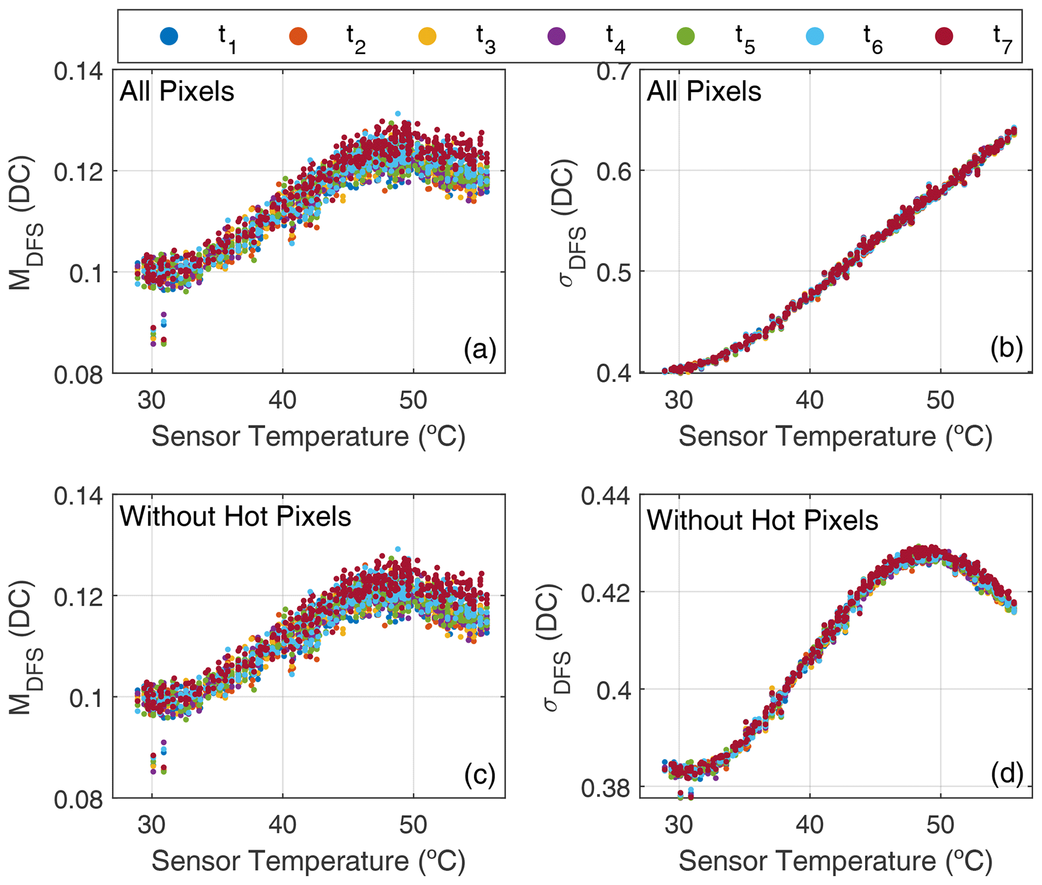
Figure 3Mean (a, c) and standard deviation (b, d) of the dark frame signal as a function of sensor temperature for different exposure times. Values in panels (a) and (b) are calculated considering all pixels and (c, d) without hot pixels.
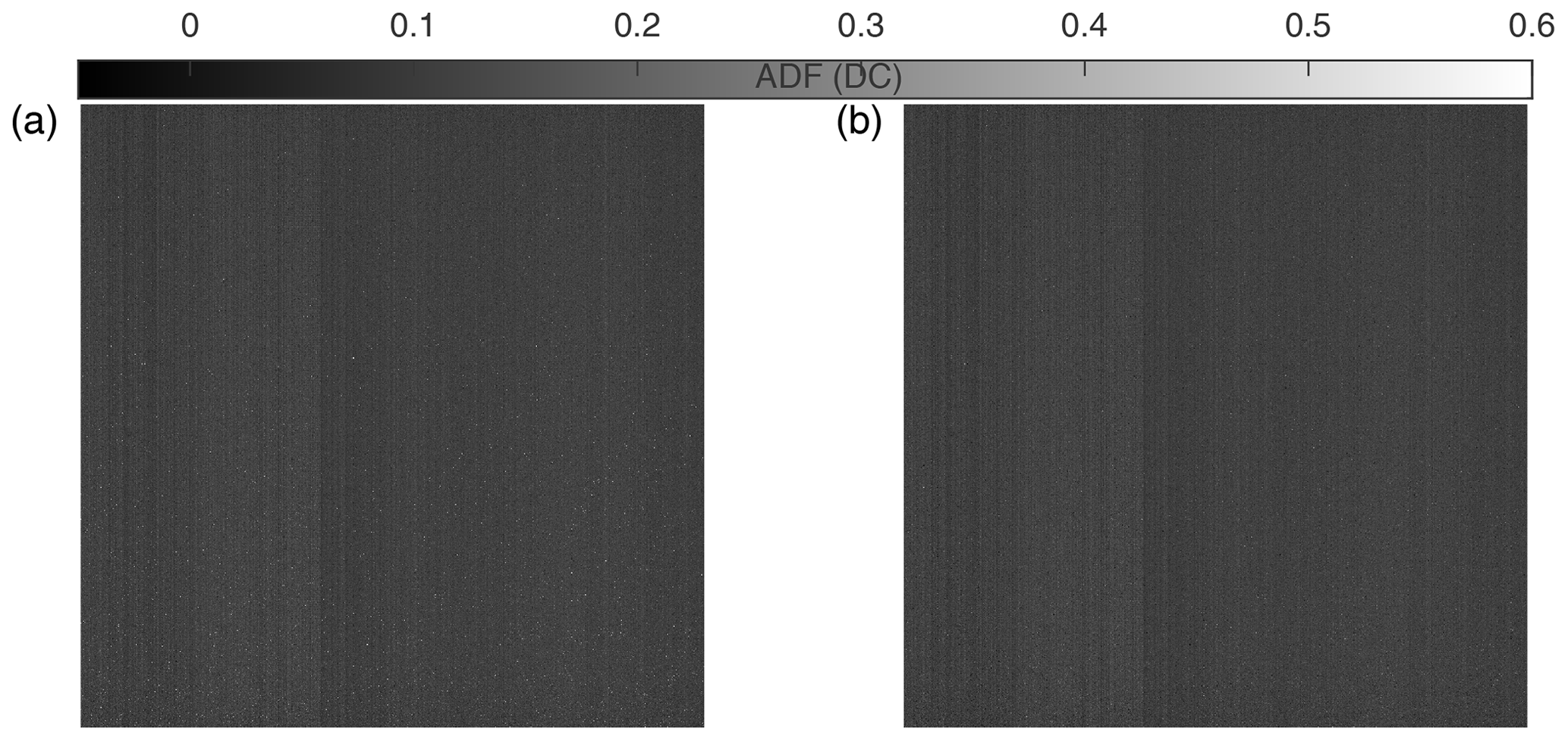
These results do not provide information about the spatial distribution of the pixel signal in a dark frame. Hence, an averaged dark frame (ADF), in which each pixel is the mean of this pixel signal in each recorded dark frame, is shown in Fig. 4a. Vertical column patterns are observed, as was also described by Román et al. (2017a), but in general with low values and without a significant signal variation, which is likely linked to the readout process of the camera. However, some pixels with a much higher signal appear in this picture; these are known as “hot pixels”.
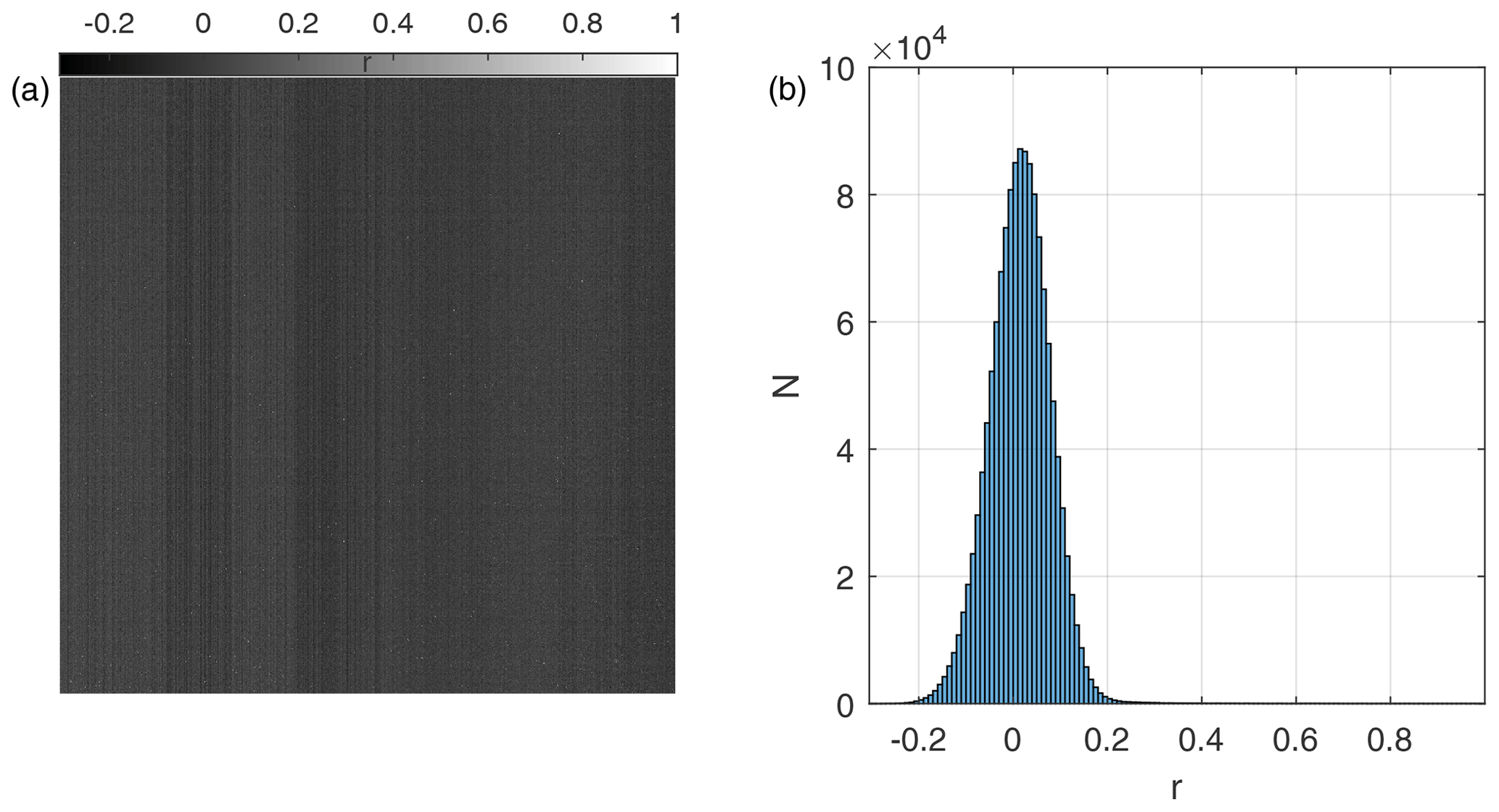
Figure 5Correlation coefficient of pixel signal at t1 with temperature for each pixel (a) and its frequency distribution (b).
The hot pixels present a high signal even without light, and this signal usually increases with increasing temperature and exposure time (Porter et al., 2008). This dependence on temperature has been used to identify and reject the hot pixels of the camera. The correlation coefficient (r) of each pixel with the temperature at each exposure time for all available dark frames has been calculated. Figure 5a shows the correlation coefficient for the t1 exposure time. The spatial distribution of this correlation coefficient is similar to the ADF, showing some column patterns but with most of the values near zero and with high values for hot pixels. In fact, the frequency distribution of this correlation coefficient, also shown for t1 in Fig. 5b, presents a Gaussian distribution centred around zero, thus indicating no correlation with temperature. However, some pixels show high r values. A threshold value to detect those outliers has been defined as the median multiplied by 2 minus the minimum of the r distribution. The pixels showing an r value higher than this threshold in any of the seven exposure times have been classified as hot pixels, and they will be excluded in the analysis of this work. A total of 2158 hot pixels (0.16 % of the total) have been detected by this method. Figure 4b shows the ADF without the identified hot pixels, and the reduction of the hot pixels is significant, indicating the good performance of the method used to detect hot pixels. Dead pixels, whose signal does not vary even under the presence of light, have not been found in the camera.
The MDFS and σDFS values have been recalculated after rejecting the identified hot pixels, and these values are also shown in Fig. 3c and d as a function of temperature. The MDFS values are similar with and without hot pixels; however, the σDFS values, associated with the readout noise, are significantly reduced when the hot pixels are discarded. Without hot pixels, σDFS shows a dependence on temperature similar to MDFS, reaching a maximum value of around 0.43 DC close to 50 ∘C. Considering this result, the readout noise (Nr) of the analysed camera has been assumed to be 0.43 DC.
Finally, for all pixel signals (excluding hot pixels) of all measured dark frames at all exposure times, 81.55 % (20.44 %, 40.64 % and 20.47 % for R, G and B) of the signals have 0 DC, 14.94 % (3.69 %, 7.56 % and 3.69 % for R, G and B) have 1 DC, and 3.51 % (0.86 %, 1.81 % and 0.84 % for R, G and B) have −1 DC. These results indicate the low readout noise of the camera since most of the signals equal zero and do not show a dependence on the channel, which is expected if the black level and white balance are corrected well.
3.4 Linear response and effective exposure times
One of the most important sensor characterizations is the linear response of the pixel signal, which mainly depends on the structure of the pixel type (Wang, 2018). This feature indicates how linear the ratio between the pixel signal and the incoming irradiation is. The linear response can be obtained by varying the intensity of a light source with a fixed exposure time for the image sensor or by increasing the exposure time (it increases the received irradiation) of the sensor at a fixed light condition (Wang, 2018). The analysed camera is installed outdoors; hence, the variation in exposure times under fixed light conditions, such as sky light for a few seconds, is more feasible than using a controllable and variable light source.
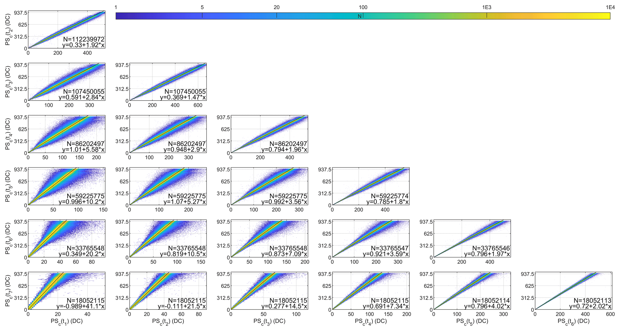
Figure 6Corrected pixel signal at different exposure times as a function of the corrected pixel signal at other exposure times for all available daytime images on 18 August 2019 at Valladolid. Saturated pixels are not included. The panels show the weighted least squares linear fit and the amount of data (N).
Debevec and Malik (1997) represented the pixel signal as a function of the exposure time to retrieve the pixel linear response, finding non-linearity at low and high pixel signal values. In our case, we have observed that the exposure times are discretized; hence, we do not know the applied exposure times with accuracy. Therefore, we have represented each corrected pixel signal (PSc) obtained at a given exposure time as a function of the same signal but captured under other exposure times (same pixel and scenario but different exposure times and hence different signals); it has been done for all combinations of two different exposure times. Pixels containing buildings or below the horizon have been masked and are not considered. Figure 6 shows these representations for the different exposure times using the pixels of all images recorded on 18 August 2019. The relationship between pixel signals at different exposure times looks linear. Pixels with (uncorrected) raw signals above 984 DC have been assumed to be saturated, and they have been removed for all images and do not appear in Fig. 6. The 984 DC threshold is based on the visual inspection of graphs similar to Fig. 6 but without saturated pixel rejection. Higher data dispersion in Fig. 6 is observed when the exposure time difference is greater among them. This data dispersion is mainly caused by the presence of moving clouds on 18 August 2019 that can quickly vary the incoming radiation to the pixels. This is confirmed by Fig. S1 in the Supplement which is similar to Fig. 6 but for a cloud-free day (17 August 2019) and where the dispersion is lower. In spite of the clouds, the amount of dispersed data in Fig. 6 is too low considering the high amount of total data (18–112 million data points depending on the panels) and the log scale of the amount of data in the density plots.
The data in Fig. 6 have been fitted to a linear regression for each panel using a weighted least squares fit. The chosen weight, w, of each data pair is the following:
where Nx and Ny represent the total noise (N) of the PSc measurement for the exposure time represented on the x and y axes, respectively. N can be described as the sum of the readout noise and the shot noise (Ns). Ns is associated with the particle nature of light and can be expressed as the square root of the measured signal caused by light (black corrected) since it follows a Poisson distribution. Hence, in this work,
The used linear fit has been chosen to weight the residual differences of a least squares fit according to the noise of the PSc data pairs. The linear fits in Fig. 6 agree well with the data, showing a high correlation with r values close to 1. The y intercept of all fits is close to zero, as expected, and it points out the goodness of the black level correction. The expected slope of each fit should be the ratio between both exposure times because the recorded signal must be proportional to the integration time; however, the obtained slopes differ from the expected values. This result indicates that surely the nominal values of the exposure times used are not equal to the real exposure times of the sensor, as we suspected due to the observed discretization.
These slope and y-intercept values have been calculated for all available days between 12 July 2018 and 1 May 2020 and only for the consecutive time exposures (cases shown in the diagonal plots of Fig. 6) because they show the lower deviation. A total of 56 d have been discarded because they show a correlation coefficient below 0.999 in at least one of the exposure times. Figure 7 shows the remaining values obtained for all periods (a total of 593 data points for exposure time relationship). The slope values do not present a significant variation in time, nor does the y intercept which has the most values below 1 DC. The amount of data used for the shorter exposure times clearly varies with the sunshine duration, while for the higher exposure times, the amount of data is always similar, which is explained by the frequent pixel saturation reached for these higher exposure times, especially as the SZA decreases.
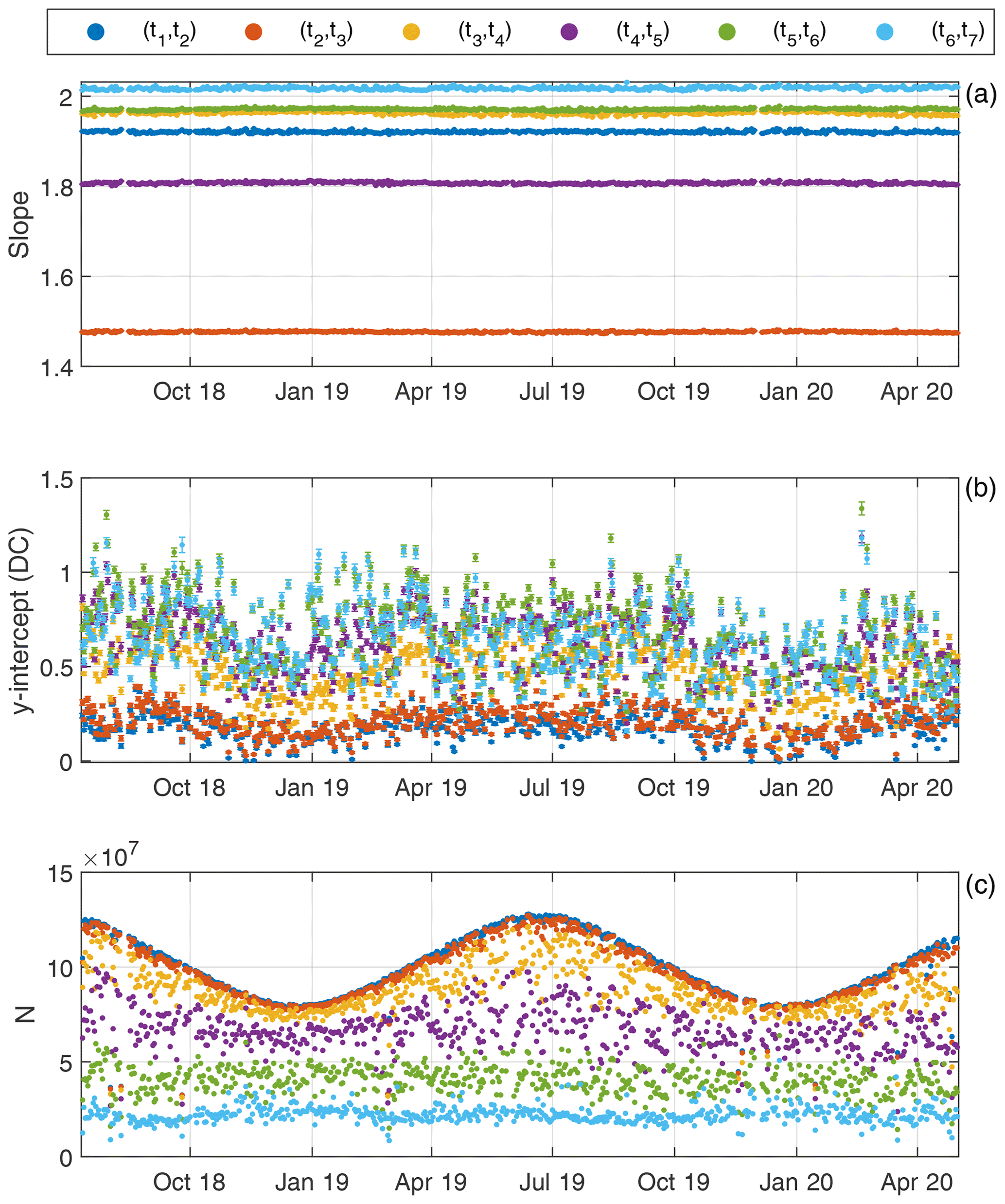
Figure 7Time evolution of the (a) slope, (b) y intercept and (c) amount of used data (N) of the daily weighted least squares linear fits for different exposure time pairs.
The slope and y-intercept correlation with the mean temperature has also been analysed, obtaining an r value ranging from −0.04 (t1, t2) to −0.69 (t5, t6) for the slope and from 0.15 (t6, t7) to 0.64 (t3, t4) for the y intercept. Despite the fact that the correlation between the slopes and temperature is not negligible, the standard deviation of the slopes is about 0.15 % for all exposure times, which indicates a low variation. The empirical relationship between two exposure times has been assumed to be the mean of the obtained slopes for these two exposure times, the assigned uncertainty being the combination of the standard deviation of the 519 obtained daily values and the propagated error in the slope values associated with the least squares fits. The obtained exposure time relationships given by the mean of the calculated slopes provide a set of relative exposure times which achieve an effective linear pixel response; hence, these relative exposure times can be assumed to be effective exposure times for linear response. The mean slope obtained for the i and j exposure times is therefore equal to the ratio between these times: .
3.5 High dynamic range linear image
The multi-exposure configuration was chosen to capture the maximum non-saturated signal of all-sky points from the brightest to the darkest with the aim to form a unique image with high dynamic range (HDR), in which the signal of each pixel will be linearly proportional to the received sky radiation. It means that in this image, the signal ratio between two pixels should be equal to the ratio of the incoming sky radiation to both pixels.
To this end, in this work only one linear HDR image has been calculated for each available image set formed by seven multi-exposure raw images. The signal of a pixel of the HDR image is the PSc of the same pixel in the image in which this pixel shows the highest signal (lowest noise) but without saturation (original signal below 985 DC); this signal is then normalized to the t3 exposure time. As an example, if a pixel reaches the highest PSc without saturation in the image with t5, then the signal assigned to this pixel in the HDR image will be the PSc in the t5 image divided by and by , both values obtained in Sect. 3.4 (the mean value of the slopes). If the highest PSc without saturation is reached in the image with t1, then the PSc in the t1 image will be multiplied by and by . The normalization to t3 instead of other times has been chosen because the most non-saturated pixels appear for exposure times between t1 and t5 (see Fig. 7c); hence, t3 reduces the number of multiplications between coefficients and hence the uncertainty. Usually one (from t2 or t4 to t3) or two (from t1 or t5 to t3) coefficient multiplications are needed. The HDR signal of the pixels showing saturation in all image sets is assumed to be the null value. The uncertainty in the HDR signal is calculated as the propagation of the uncertainties of PSc and of the applied coefficients to t3 normalization.
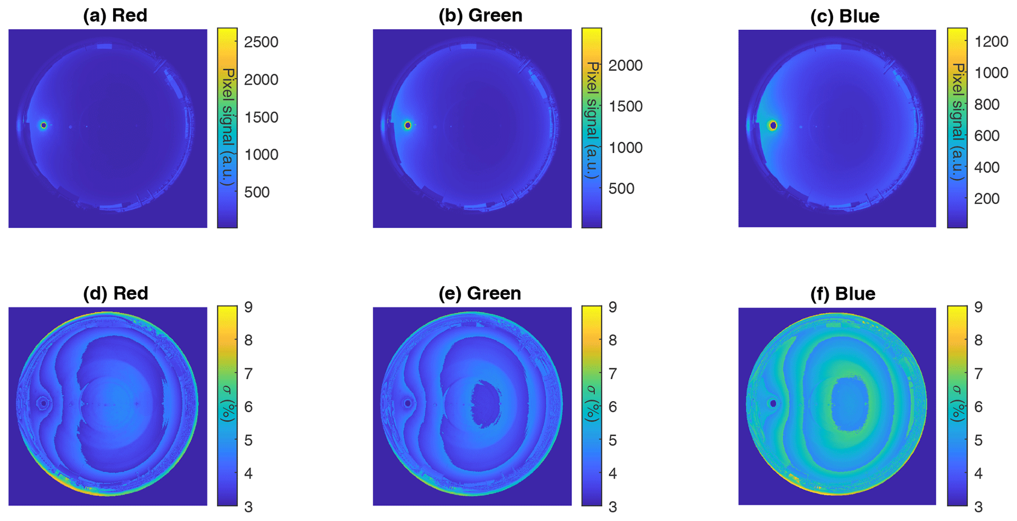
Figure 8Linear HDR pixel signal (a–c) and its uncertainty (d–f) for the red (a, d), green (b, e) and blue (c, f) channels at Valladolid on 17 August 2019 at 07:25 UTC.
Figure 8 shows an example of the calculated HDR signal and its propagated uncertainty for each channel at Valladolid on 17 August 2018 at 07:25 UTC (same case as Fig. 2). The Sun appears saturated in the three channels due to the high value of solar radiation even in the lowest exposure time. The blue channel presents higher values (regarding the maximum values) in the sky than the other channels; it is expected due to the bluish sky colour. The differences in the arbitrary unit scale between the three channels are caused by the white balance correction which makes the red channel reach higher values than green and blue. The higher uncertainty in the blue channel (mostly between 4.5 % and 6.5 %) is caused by the same reason. The uncertainty in the red and green channels ranges from 3.5 % to 4.5 %, but it shows a circular pattern in the middle of the image, especially for the red channel, which is not clearly appreciated in the blue channel. This could be related to the formation of a reflected image of part of the camera in the dome, as can be seen in Fig. 2.
The retrieved HDR images are 2D with only one colour assigned to each pixel. This is enough to extract relative radiances, but to visualize a colour image of the captured scene can be helpful for other applications. To this end, an RGB colour HDR has been retrieved from the HDR by a demosaicing algorithm (Li et al., 2008) which converts the Bayer-pattern-encoded image into a true-colour image. The signal of this colour HDR image is still linear; hence, its direct representation could only show the brightest areas of the sky. Therefore, a tone mapping (Salih et al., 2012) has been applied to this colour HDR to include all the dynamic ranges in the scale. As a result, Fig. 2c shows the tone map of a colour HDR image. This image shows the solar aureole and the sky without saturation and with enough brightness. However, it looks greenish in comparison to the real sky. It is because in the HDR the white balance is not applied (it has been removed in the PSc). To solve that, the blue and green channels of the colour HDR image have been multiplied by WBSFB (by 1.1) and WBSFG (by 2.1), respectively, to apply the original white balance. The result is presented in Fig. 2d, which shows a more realistic blue sky. This result indicates that the white balance can be applied after the raw image is captured instead of before, giving a similar result but avoiding the saturation of several pixels and not reducing the dynamic range of the channels.
3.6 Extraction of relative sky radiance
Once a linear HDR image has been calculated, the relative sky radiance at any sky point can be extracted. The term “relative radiance” in this work refers to uncalibrated sky radiance measurements; i.e. it is the sky radiance but in arbitrary units instead of watts per metre squared per steradian () or physically equivalent units. First, all the HDR pixel signals are divided by their field of view to obtain radiance units, which is the signal per solid angle (sr−1). Then, for a sky point defined by its zenith and azimuth coordinates, the great-circle distance between its coordinates and the coordinates viewed by each pixel is computed, and the camera pixel showing the lowest great-circle distance is assumed to be the pixel pointing to this sky point. This obtained pixel is only representative of one channel (R, G or B), and its signal could be noisy; hence, a disc with radius of 3 pixels centred around the obtained pixel (a total of 37 pixels) is chosen to include the three channels. The chosen 37 pixels are separated by channel, and their HDR signals are averaged, obtaining the sky radiance for a sky point at the three channels. The uncertainty of these radiances is also calculated by the propagation of the HDR signal uncertainty of each pixel.
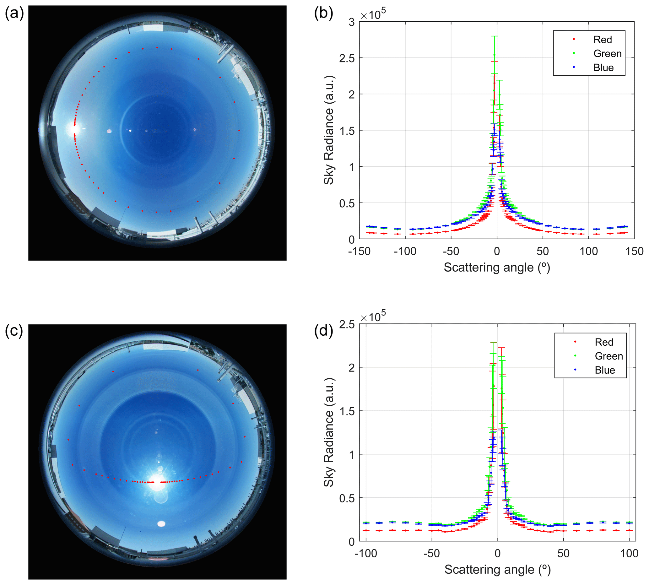
Figure 9Camera sky radiance at the three channels (b, d) for almucantar (a, b) and hybrid (c, d) scans on 17 August at 07:25 UTC and 12:25 UTC, respectively. Panels (a) and (c) show in red the almucantar and hybrid sky points on a tone map of the demosaiced HDR image.
Figure 9 shows the extracted relative sky radiance at the three camera channels for one AERONET almucantar and one AERONET hybrid scan. The sky points have been marked in the left panels, clarifying the geometry of these scans. The obtained radiances are symmetric with respect to the Sun's position, as expected under cloudless conditions, showing higher radiance and uncertainty values for the lower scattering angles (solar aureole). This symmetry with respect to the Sun is useful to discard cloud-contaminated data (Román et al., 2017b). To compare this with photometer measurements, we have extracted the sky radiances at the same left and right points as the AERONET almucantar and hybrid scenarios, and both left and right radiance pairs have been averaged for each channel. The values showing differences above 20 % between the left and right radiances have been classified as cloud-contaminated and removed. This average and cloud-screening process, based on Holben et al. (1998, 2006), has also been applied to the AERONET sky radiances.
4.1 Camera vs. photometer
A comparison of the all-sky camera radiances with the measured photometer sky radiances has been done to evaluate the performance of the proposed methodology (Sect. 3). Camera effective wavelengths are not equal to the photometer, but, in a first approximation, radiances at 440, 500 and 675 nm have been assumed to be at 467 (blue), 536 (green) and 605 nm (red), respectively. The photometer and all-sky camera data used for comparison were recorded from July 2018 to March 2020. For each available AERONET almucantar and hybrid scenario, the closest HDR image within a ±2.5 min window has been found, and the sky radiance at cloud-free points of the chosen scenario has been extracted from this image. For almucantar scans, the point at azimuth equal to 180∘ has been discarded since the symmetry check for cloud screening cannot be applied.
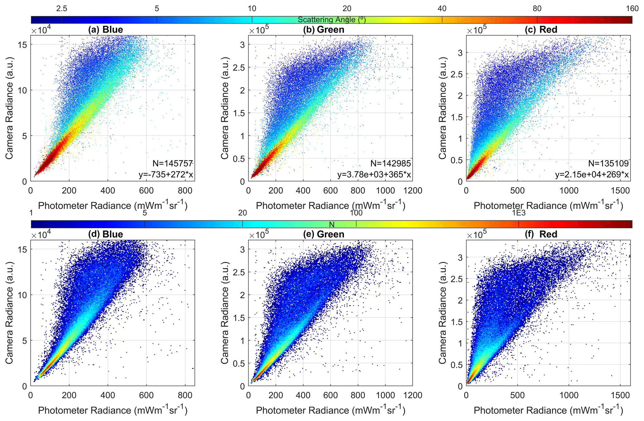
Figure 10Camera sky radiance as a function of photometer radiances for blue (a, d), green (b, e) and red (c, f) channels. Colour scale represents the scattering angle in panels (a)–(c), while it means the amount of available data N in an interval (density plot) in panels (d)–(f).
The camera radiance against photometer data is shown in Fig. 10 for each channel. The signal between camera and photometer radiances correlates with r values of 0.90, 0.88 and 0.80 for blue, green and red channels, respectively. However, there are several data pairs showing higher camera radiances than photometer ones. These deviated data correspond to scattering angles below 10∘ as indicated by the colour scale. Most of the data present a linear behaviour as shown by the density plots of Fig. 10, suggesting a linear relationship between radiances if the scattering angles below 10∘ are discarded. The correlation coefficients rise to 0.98, 0.98 and 0.97 for blue, green and red channels, respectively, if scattering angles below 10∘ are not considered. The worse performance of the lowest scattering angles is not caused by problems in the linearity of HDR images, especially for high signal values, because higher scattering angles show also high radiance values, but these ones fit well with the photometer measurements. Some observed light reflections in the camera dome and lens near the solar aureole image could be mainly responsible for the results obtained for scattering angles below 10∘. These angles will not be considered hereafter.
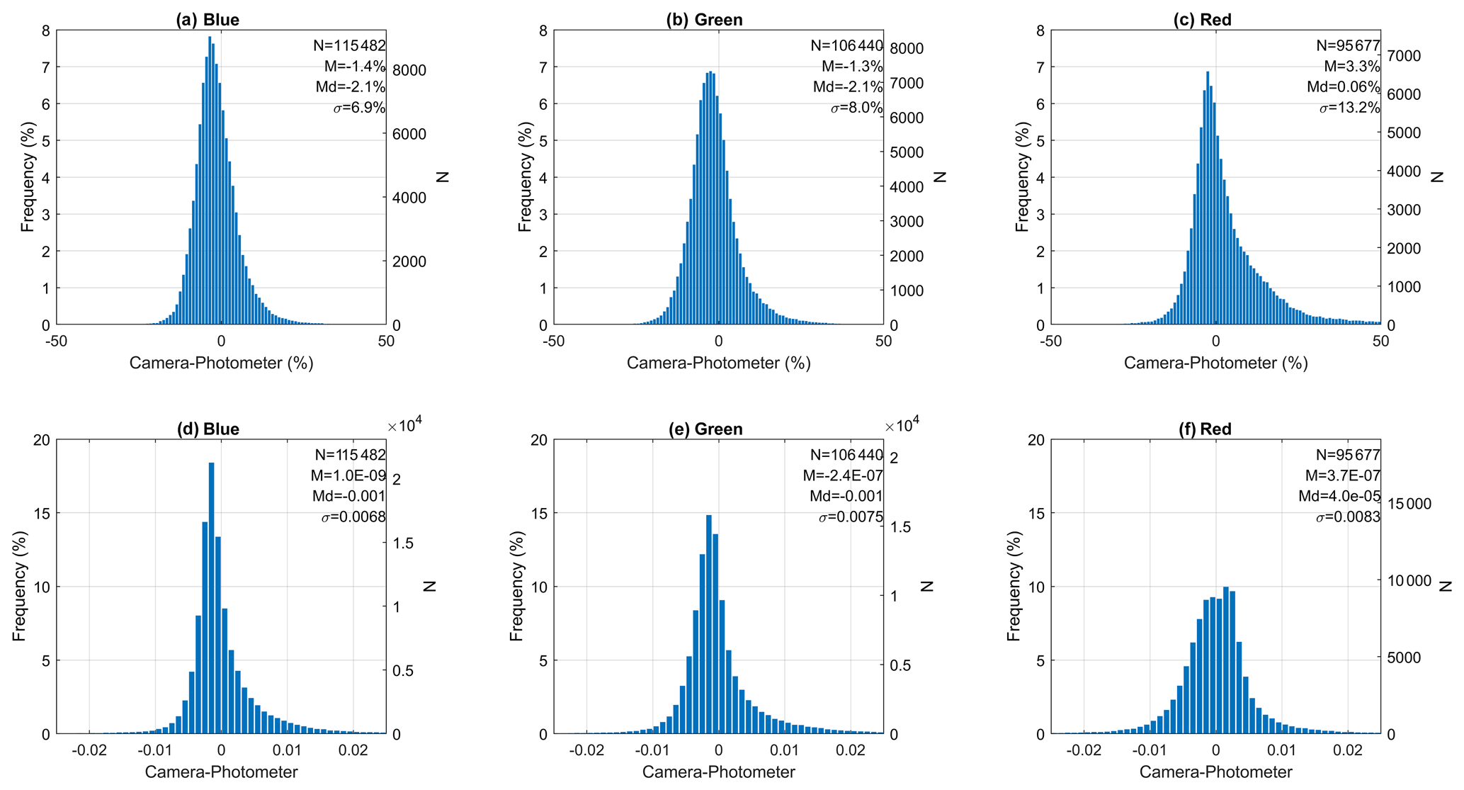
Figure 11Frequency histograms of the relative (a–c) and absolute (d–f) differences between the camera and photometer normalized sky radiances for blue (a, d), green (b, e) and red (c, f) channels, respectively. Radiances with scattering angles below 10∘ are not considered. The amount of data (N), the mean (M), median (Md) and standard deviation (σ) of the differences are also included.
In order to compare camera and photometer radiances in a quantitative way, both radiances have been normalized. To this end, for each measurement group (almucantar or hybrid scenario) and channel, only the radiance points classified as cloud-free in both photometer and camera have been selected. Then, each radiance value of a given scenario and channel has been divided by the sum of all radiances at this channel. The sum of all normalized sky radiances at one channel must be equal to 1 for each measurement group. These normalized radiances give relative information about sky radiance distribution and are useful for retrieving some aerosol properties (Román et al., 2017a). The correlation between camera and photometer normalized radiances is 0.99 for the three channels. Figure 11 presents the frequency histograms of the relative and absolute differences between the camera and photometer normalized radiances (excluding scattering angles below 10∘). The difference distributions show a Gaussian behaviour with the maximum value around zero but slightly shifted to negative values except the absolute distribution of the red channel. The negative mean of about −1.3 % in the blue and green channels indicates a camera radiance underestimation of the photometer radiances at these channels. The red channel shows an overestimation by the camera of about 3 % which is likely caused by the positive tail shown in the distribution. The mean of the absolute distributions is about 0. The standard deviation, associated with the uncertainty, ranges from 6.9 % (blue) to 13.2 % (red).
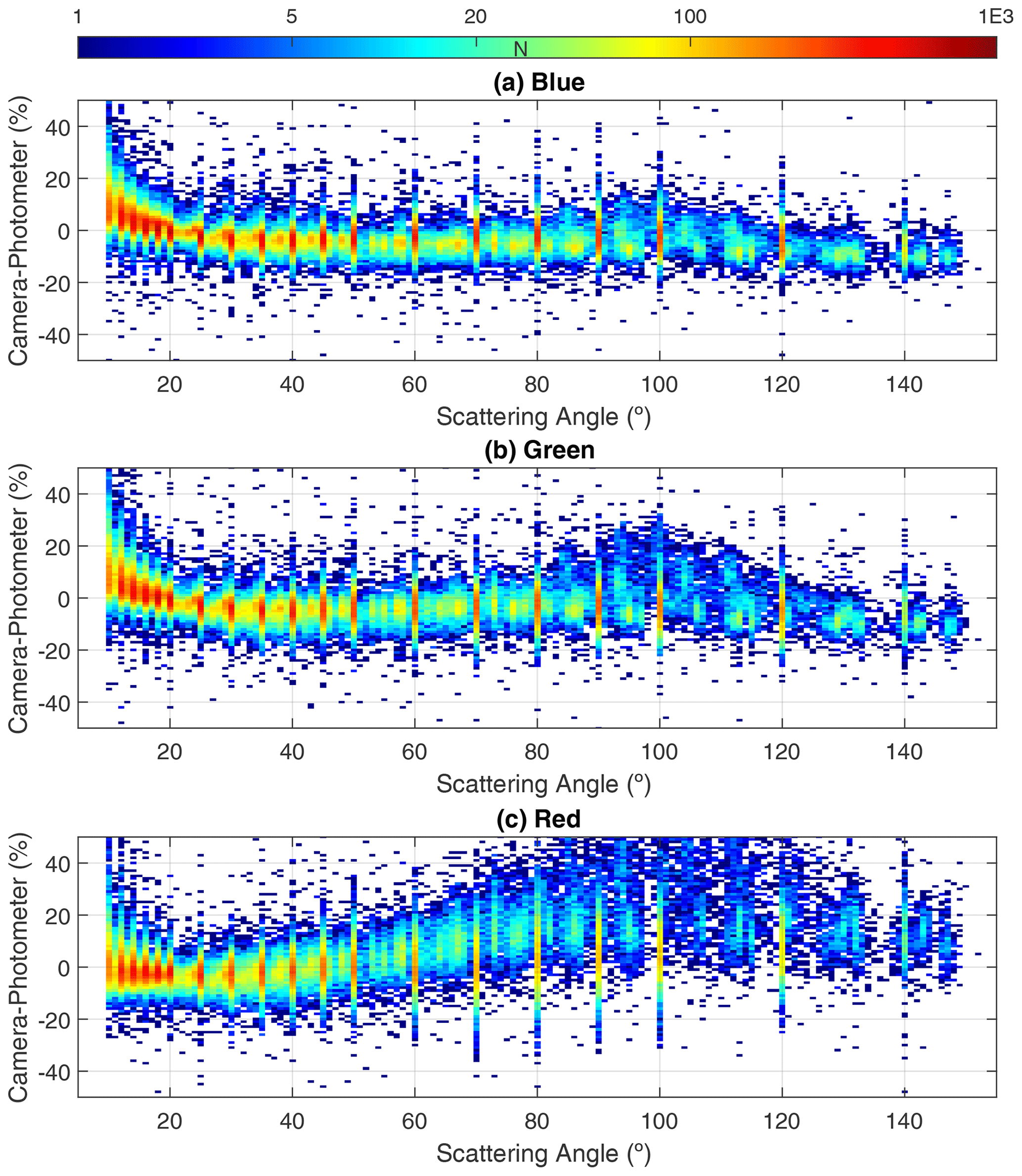
Figure 12Relative differences between the camera and photometer normalized radiances as a function of the scattering angle for blue (a), green (b) and red (c) channels. Radiances with scattering angles below 10∘ are not considered.
Figure 12 presents these differences as a function of scattering angle. These density plots show higher density at specific angles because the AERONET hybrid scans are always done at the same scattering angles, while AERONET almucantar scans are measured at fixed azimuth angles, and therefore the scattering angle also depends on the SZA. In general, the camera radiances overestimate/underestimate the photometer ones for the lowest/greatest scattering angles for the blue and green channels. The differences for the red channel are around zero for the lowest angles, but the camera radiances strongly overestimate the photometer ones for scattering angles above 70∘, especially in the almucantar scenario.
4.2 Camera vs. simulations
Part of the obtained differences and this variation with scattering angle could be caused by the differences between camera and photometer wavelengths (e.g. in the red channel, this difference is about 70 nm). To solve that, sky radiances at the same camera effective wavelengths have been simulated with the radiative transfer model of the forward module of the GRASP algorithm (Generalized Retrieval of Atmosphere and Surface Properties; Dubovik et al., 2014). The main inputs in this model have been obtained from AERONET retrievals: aerosol size distribution in 22 size bins, real and imaginary refractive index at 440, 675 and 870 nm linearly interpolated to camera wavelengths, and sphericity factor. Only AERONET retrievals satisfying an inversion error below 10 % in the sky radiances have been used. Valladolid climatological values of the bidirectional reflectance distribution function (BRDF) parameters, obtained from the MODIS MCD43C1 (Schaff et al., 2011) satellite product (see Román et al., 2018), have been interpolated to camera wavelengths and used as input in GRASP. With this information, the radiative transfer model is capable of simulating the sky radiance at any desired sky direction; in our case, these points have been selected to match the AERONET almucantar and hybrid scans separately.
First, the performance of the radiative transfer simulations has been evaluated against photometer data by simulating sky radiances at 440, 500 and 675 nm. The data used are from July 2018 to March 2020, and each simulated scan has been directly compared with the temporally closest photometer cloud-free radiance scan. It means that we are comparing the radiance obtained by certain aerosol properties with the sky radiance used to retrieve those aerosol properties. In this case, the simulated and measured radiances agree with r values of 1.00 for the three wavelengths and without any dependence on scattering angle even for scattering angles below 10∘ (not shown). The differences between simulated and photometer normalized radiances (rejecting scattering angles below 10∘) shows a mean value of about 0.2 %, 0.4 % and 0.7 % and a standard deviation of about 2.3 %, 2.8 % and 3.2 % for 440, 500 and 675 nm, respectively. These results are within the nominal calibration uncertainty of the AERONET radiance measurements.
The radiances at almucantar (which is measured only for ) and hybrid points have been separately simulated for the HDR sky images that are closest in time (within 10 min) to the available aerosol AERONET retrievals (with sky error below 10 %) from July 2018 to March 2020. A direct comparison between camera and simulated radiances (not shown) presents worse agreement for scattering angles below 10∘ but also reveals higher r values: 0.94, 0.92 and 0.91 for 467, 536 and 605 nm, respectively. These r values rise to 0.99, 0.99 and 0.98 when scattering angles below 10∘ are not considered and to 0.99 for all wavelengths when the radiances are also normalized.
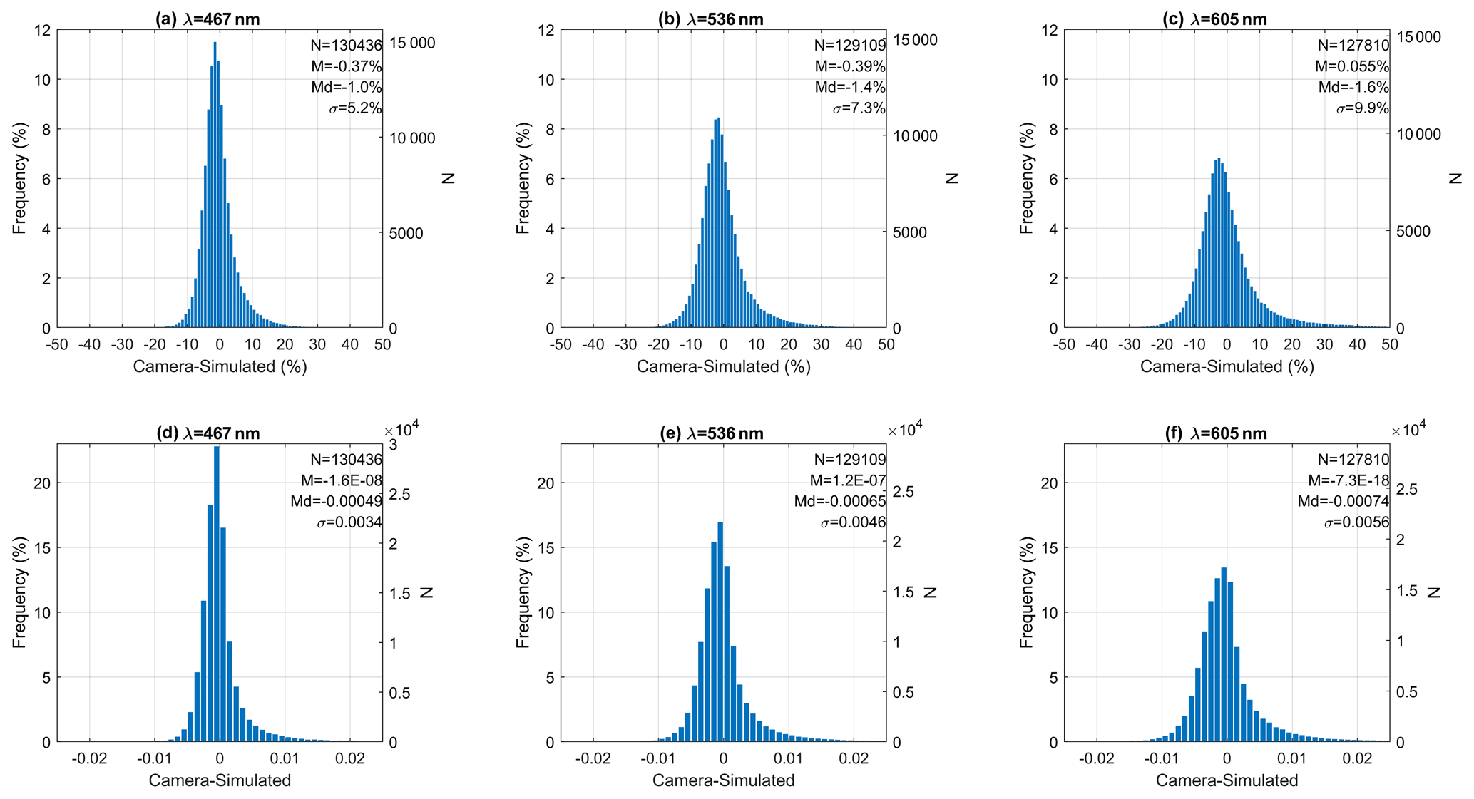
Figure 13Frequency histograms of the relative (a–c) and absolute (d–f) differences between the camera and simulated normalized sky radiances for 467 nm (a, d), 536 nm (b, e) and 605 nm (c, f). Radiances with scattering angles below 10∘ are not considered. The amount of data (N), the mean (M), median (Md) and standard deviation (σ) of the differences are also included.
Figure 13 shows the distribution of the normalized radiance differences between camera and simulations. These distributions also show a Gaussian behaviour, as was observed in the camera–photometer comparison. However, the mean and standard deviation are significantly lower. The mean values are about zero, indicating no over- or underestimation, and the standard deviation values reveal an uncertainty in camera radiances of about 5.2 %, 7.3 % and 9.9 % for 467, 536 and 605 nm, respectively. This observed improvement in the correlation and in the mean and standard deviation of the obtained differences points out the influence of the wavelength differences on the camera–photometer comparison.
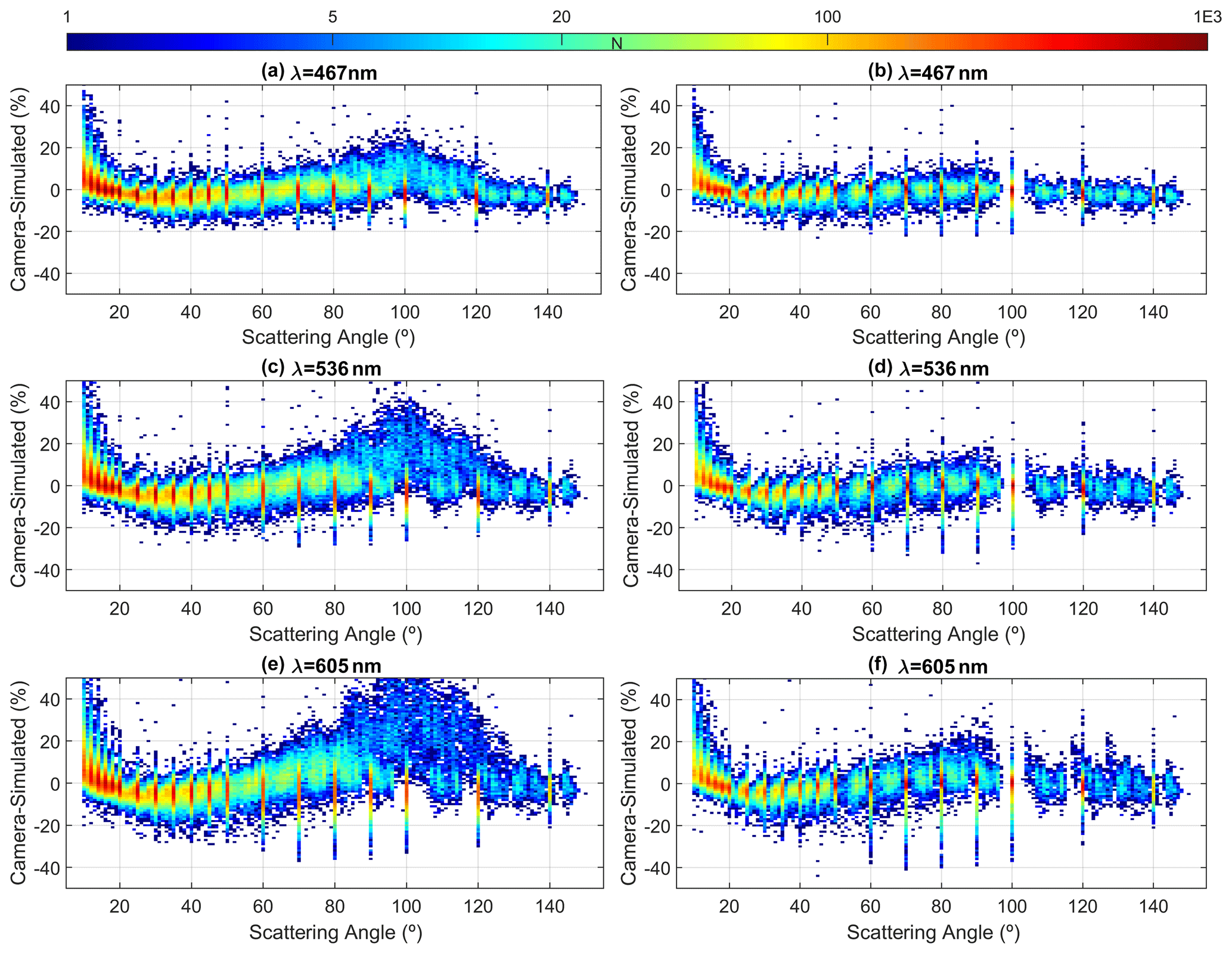
Figure 14Relative differences between the camera and simulated normalized radiances as a function of the scattering angle for 467 nm (a, b), 536 nm (c, d) and 605 nm (e, f). Left panels show the differences calculated without radiances under scattering angles below 10∘, while right panels show the same differences but also obtained without radiances under zenith angles between 48 and 65∘.
The left panels of Fig. 14 represent the dependence on scattering angle of the camera-simulated differences in normalized radiance. The behaviour is similar to the one obtained using photometer measurements instead of simulations, except for 605 nm for which the camera also overestimates the simulations for the lowest angles. High difference values appear from 80 to 120∘ scattering angles, especially at 605 nm and for almucantar scans, which is also observed in Fig. 12. These differences appear for points with zenith angles from 48 to 65∘, which corresponds with the position of the observed ring image reflected on the dome (see Figs. 2 and 9); this is an image of a piece of the prototype camera that lost part of its black colour. The right panels of Fig. 14 show the differences for normalized radiances computed without the points in the 48–65∘ zenith angle range. The high differences previously observed around the 80–120∘ scattering angles disappear if the mentioned observation angles are not considered. Under these conditions (no zenith angles from 48 to 65∘), the normalized camera radiances show a slight overestimation compared to the simulated values for scattering values below 15∘. The dependence on scattering angle is stronger for 605 nm, while for 467 nm, this dependence is not clear except for the lowest angles.
The mean of the differences between camera-simulated radiance is between −0.6 % and −0.1 % for the three channels when the points affected by the reflection in the dome are discarded; for these conditions, the standard deviation is reduced to 4.4 %, 5.7 % and 6.9 % for 467, 536 and 605 nm, respectively. For the same conditions (no scattering angles below 10∘ nor zenith points between 48 and 65∘) but applying a stronger cloud-free threshold of 5 % instead of 20 %, the amount of available data is reduced to 86 %, 80 % and 74 %, but the standard deviation goes down to 3.5 %, 4.5 % and 5.6 % for 467, 536 and 605 nm, respectively, while the mean difference values are still close to zero (between −0.4 % and −0.1 %) for the three channels. Under these conditions, 74 % (467 nm), 67 % (536 nm) and 64 % (605 nm) of the obtained camera-simulated radiance differences are within the combined uncertainty associated with the camera and simulation values; these percentages of data rise to 93 %, 89 % and 88 % for the expanded uncertainty (double the combined uncertainty). Both obtained values are about 69 % and 95 %, which are the expected values for a Gaussian distribution with a standard deviation equal to the uncertainty. This result indicates that the uncertainty associated with the camera radiances could be representative of the real camera uncertainty if the problematic camera angles are not used.
Finally, if the camera radiances with a propagated uncertainty above 5 % are also rejected (less than 0.5 % of total data), the differences in camera-simulated radiances present mean values ranging from −0.3 % to −0.1 %, median values of −0.4 %, −0.5 % and −0.4 %, and standard deviation values of 3.3 %, 4.3 % and 5.3 % for 467, 536 and 605 nm, respectively. The rejection of camera radiances with a propagated uncertainty (inherent to both HDR image calculation and radiance extraction method) above 5 % also reduces the amount of data outliers observed for scattering angles below 10∘. In this sense, the differences in the camera-simulated radiances have been calculated by applying all the mentioned quality criteria (rejection of points contaminated by camera reflections; cloud-free criterion based on differences within 5 % between symmetric points; required camera radiance uncertainty below 5 %) but rejecting only scattering angles below 8, 7 and 6∘. As result, for 467 nm, 536 and 705 nm the standard deviation of the differences are 4.0 %, 5.0 % and 5.8 % (with mean values between −0.7 % and −0.5 %) discarding angles below 8∘, 4.5 %, 5.4 % and 6.1 % (with mean values between −0.9 % and −0.7 %) discarding angles below 7∘, and 5.5 %, 5.8 % and 6.5 % (with mean values between −1.1 % and −1.0 %) discarding angles below 6∘. In this case, camera radiances overestimate the simulated ones at the lowest angles and underestimate the simulations for the rest of the angles; this fact leads to the observed increase (in absolute value) in the mean camera-simulated differences. Therefore, the use of the normalized sky radiances in this work is more appropriate without the scattering angles below 10∘. However, sky radiance at low scattering angles could be useful for some purposes such as aerosol retrieval. The uncertainty estimates provided here should be considered in the retrieval.
The present work proposes a new methodology to obtain the relative (normalized) sky radiances and their uncertainty from all-sky camera images. To this end, an all-sky camera (SONA202-NF) equipped with three spectral channels (narrower than usual) and with effective wavelengths of 467, 536 and 605 nm has been used in this paper. The proposed method only requires sky images and a set of camera images under dark conditions, both at various exposure times. Dark frames are useful to characterize the camera readout noise and black level, but any white balance correction must be avoided to this end. Hot pixels can be detected through the correlation between the pixel dark signal and temperature. The linear response of pixel signal can be characterized by taking images with different exposure times; previous knowledge of these exposure times is not necessary since the ratio between them can be calculated as the slope of a linear fit between the pixel signals at two different exposure times. These slopes give a relationship between exposure times that provide an effective linear response for the sensor. The characterization of these parameters has allowed for the calculation of a linear HDR image and then a relative sky radiance map and its uncertainty at the three camera spectral channels. The relative sky radiance at any sky direction can be extracted from these maps.
The relative sky radiance obtained by the proposed method has been compared with the radiances measured by a CE318-T photometer at the closest wavelengths of 440, 500 and 675 nm. Both radiances agree on the three wavelengths except for scattering angles below 10∘ which could be mainly caused by solar light reflections in the fisheye lens and camera dome near the Sun's position. The distribution of the differences between normalized sky radiances has shown standard deviations from 7 % (467 nm) to 13 % (605 nm), part of these differences being caused by the differences in both instrument wavelengths.
To solve the wavelength shift between instruments, the camera radiances have been compared against radiance simulations at the same wavelengths using the AERONET aerosol properties as input in a radiative transfer model. This comparison reveals an uncertainty in normalized all-sky camera radiances with scattering angles above or equal to 10∘ of about 5 %, 7 % and 10 % for 467, 536 and 605 nm, respectively. However, this uncertainty is reduced to 3.3 % (467 nm), 4.3 % (536 nm) and 5.3 % (605 nm) if the following quality criteria are applied: rejection of radiances under scattering angles below 10∘, radiance assumed to be cloud-free only when left–right symmetric data pairs show differences below 5 %, exclusion of radiances with a propagated uncertainty above 5 %, and rejection of radiance values with zenith angles between 48 and 65∘ which encompass an area contaminated by a reflected image of part of the camera. The normalized camera sky radiance slightly overestimates the simulations at the lowest scattering angles.
With the obtained results, we make two recommendations for all-sky camera manufactures: (1) the application of white balance should be done after the capture of the raw image instead of before because it avoids unnecessary pixel saturations and reduces the shot noise and (2) the reduction of reflected images in the fisheye lens and camera dome which can contaminate the sky radiance maps. The spectral filter width reduction on the SONA202-NF camera filters allows for the use of all-sky cameras for novel approaches; narrower filters would be more helpful in the future since in the current filter set-up, some colour channels are still sensitive to wavelengths associated with the other channels.
The camera relative sky radiances obtained could be calibrated in absolute physical units, but this was out of the scope of this paper. The determination of normalized sky radiances is useful for the retrieval of aerosol properties. Therefore, we will try to use these kinds of measurements in the future in combination with other instruments to retrieve aerosol properties like the particle size distribution. Finally, we encourage other researchers interested in sky radiance data to apply the developed method to their all-sky cameras to obtain relative sky radiance maps.
The code used is available upon request to the authors.
AERONET data are publicly available on the AERONET web page (https://aeronet.gsfc.nasa.gov/, last access: 8 March 2021, NASA, 2021). Sky camera images and products are available upon request to the authors.
The supplement related to this article is available online at: https://doi.org/10.5194/amt-14-2201-2021-supplement.
JCAS and RR designed and developed the main concepts and ideas behind this work and wrote the paper with input from all authors. They also ran the different irradiance/radiance simulations. CL developed and provided the all-sky camera used. RG was responsible for the camera's operation at the Valladolid station. VEC and CT were responsible for the Valladolid AERONET station used. DM, AC and AMdF contributed in the interpretation of the results.
The authors declare that they have no conflict of interest.
The authors thank the Spanish Ministry of Science, Innovation and Universities for the support through the ePOLAAR project (RTI2018-097864-B-I00). The authors acknowledge the use of GRASP inversion algorithm software (https://www.grasp-open.com, last access: 3 March 2021) in this work and also thank the team of GRASP SAS for the GRASP code support and training. LibRadtran developers are also acknowledged for the use of their code. The authors gratefully thank AERONET for the aerosol products used. Finally, the authors thank the GOA-UVa staff members who helped with the maintenance task of the instruments used and the support of station infrastructure.
This research has been supported by the Ministerio de Ciencia, Innovación y Universidades (grant no. RTI2018-097864-B-I00) and by Junta de Castilla y León (grant no. VA227P20).
This paper was edited by Daniel Perez-Ramirez and reviewed by two anonymous referees.
Alonso-Montesinos, J., Batlles, F. J., and Portillo, C.: Solar irradiance forecasting at one-minute intervals for different sky conditions using sky camera images, Energ. Convers. Manage., 105, 1166–1177, 2015.
Antuña-Sánchez, J. C., Roman, R., Bosch, J. L., Toledano, C., Mateos, D., González, R., Cachorro, V., and de Frutos, A.: ORION software tool for the geometrical calibration of all-sky cameras, in preparation, 2021.
Barbieri, F., Rajakaruna, S., and Ghosh, A.: Very short-term photovoltaic power forecasting with cloud modeling: A review, Renew. Sust. Energ. Rev., 75, 242–263, 2017.
Bennouna, Y. S., Cachorro, V. E., Torres, B., Toledano, C., Berjón, A., De Frutos, A. M., and Coppel, I. A. F.: Atmospheric turbidity determined by the annual cycle of the aerosol optical depth over north-center Spain from ground (AERONET) and satellite (MODIS), Atmos. Environ., 67, 352–364, 2013.
Cachorro, V. E., Burgos, M. A., Mateos, D., Toledano, C., Bennouna, Y., Torres, B., de Frutos, Á. M., and Herguedas, Á.: Inventory of African desert dust events in the north-central Iberian Peninsula in 2003–2014 based on sun-photometer–AERONET and particulate-mass–EMEP data, Atmos. Chem. Phys., 16, 8227–8248, https://doi.org/10.5194/acp-16-8227-2016, 2016.
Cazorla, A., Olmo, F. J., and Alados-Arboledas, L.: Using a sky imager for aerosol characterization, Atmos. Environ. 42, 2739–2745, https://doi.org/10.1016/j.atmosenv.2007.06.016, 2008.
Coulson, K. L.: Polarization and Intensity of Light in the Atmosphere, A Deepak Pub, ISBN 9780937194126, 1988.
Debevec, P. E. and Malik, J.: Recovering high dynamic range radiance maps from photographs, in: Proceedings of the 24th Annual Conference on Computer Graphics and Interactive Techniques, ACM Press/Addison-Wesley Publishing Co., USA, 369–378, https://doi.org/10.1145/258734.258884, 1997.
Dubovik, O. and King, M. D.: A flexible inversion algorithm for retrieval of aerosol optical properties from sun and sky radiance measurements, J. Geophys. Res.-Atmos. 105, 20673–20696, 2000.
Dubovik, O., Lapyonok, T., Litvinov, P., Herman, M., Fuertes, D., Ducos, F., Lopatin, A., Chaikovsky, A., Torres, B., Derimian, Y., Huang, X., Aspetsberger, M., and Federspiel, C.: GRASP: A Versatile Algorithm for Characterizing the Atmosphere, SPIE, Newsroom, https://doi.org/10.1117/2.1201408.005558, 2014.
Dubovik, O., Smirnov, A., Holben, B. N., King, M. D., Kaufman, Y. J., Eck, T. F., and Slutsker, I.: Accuracy assessments of aerosol optical properties retrieved from Aerosol Robotic Network (AERONET) sun and sky radiance measurements, J. Geophys. Res.-Atmos., 105, 9791–9806, 2000.
Holben, B. N., Eck, T. F., Slutsker, I., Tanré, D., Buis, J. P., Setzer, A., Vermote, E., Reagan, J. A., Kaufman, Y. J., Nakajima, T., Lavenu, F., Jankowiak, I., and Smirnov, A.: AERONET – a federated instrument network and data archive for aerosol characterization, Remote Sens. Environ. 66, 1–16, 1998.
Holben, B. N., Eck, T. F., Slutsker, I., Smirnov, A., Sinyuk, A., Schafer, J., Giles, D., and Dubovik, O.: AERONET's version 2.0 quality assurance criteria, in: Remote Sensing of the Atmosphere and Clouds, edited by: Tsay, S.-C., Nakajima, T., Singh. R. P., and Sridharan, R., SPIE, 6408, 134–147, https://doi.org/10.1117/12.706524, 2006.
Kholopov, G. K.: Calculation of the effective wavelength of a measuring system. J. Appl. Spectrosc., 23, 1146–1147, https://doi.org/10.1007/BF00611771, 1975.
Li, D. H. W. and Lam, T. N. T.: Determining the optimum tilt angle and orientation for solar energy collection based on measured solar radiance data, Int. J. Photoenergy, 2007, 085402, https://doi.org/10.1155/2007/85402, 2007.
Li, X., Gunturk, B., and Zhang, L.: Image demosaicing: a systematic survey, in: Visual Communications and Image Processing 2008, edited by: Pearlman, W. A., Woods, J. W., and Lu, L., SPIE, 489–503, https://doi.org/10.1117/12.766768, 2008.
Mayer, B. and Kylling, A.: Technical note: The libRadtran software package for radiative transfer calculations – description and examples of use, Atmos. Chem. Phys., 5, 1855–1877, https://doi.org/10.5194/acp-5-1855-2005, 2005.
Nakajima, T., Tonna, G., Rao, R., Boi, P., Kaufman, Y., and Holben, B.: Use of sky brightness measurements from ground for remote sensing of particulate polydispersions, Appl. Optics, 35, 2672–2686, 1996.
NASA: AERONET, available at: https://aeronet.gsfc.nasa.gov/, last access: 8 March 2021.
Porter, W. C., Koop, B., Dunlap, J. C., Widenhorn, R., and Bodegom, E.: Dark current measurements in a CMOS imager, in: Sensors, Cameras, and Systems for Industrial/Scientific Applications IX, edited by: Blouke, M. M. and Bodegom, E., SPIE, 98–105, https://doi.org/10.1117/12.769079, 2008.
Román, R., Antón, M., Cazorla, A., de Miguel, A., Olmo, F. J., Bilbao, J., and Alados-Arboledas, L.: Calibration of an all-sky camera for obtaining sky radiance at three wavelengths, Atmos. Meas. Tech., 5, 2013–2024, https://doi.org/10.5194/amt-5-2013-2012, 2012.
Román, R., Bilbao, J., and de Miguel, A.: Uncertainty and variability in 824 satellite-based water vapor column, aerosol optical depth and Angström Exponent, and its effect on radiative transfer simulations in the Iberian Peninsula, Atmos. Environ., 89, 556–569, 2014.
Román, R., Torres, B., Fuertes, D., Cachorro, V. E., Dubovik, O., Toledano, C., Cazorla, A., Barreto, A., Bosch, J. L., Lapyonok, T., González, R., Goloub, P., Perrone, M. R., Olmo, F. J., de Frutos, A., and Alados-Arboledas, L.: Remote sensing of lunar aureole with a sky camera: Adding information in the nocturnal retrieval of aerosol properties with GRASP code, Remote Sens. Environ., 196, 238–252,1126, https://doi.org/10.1016/j.rse.2017.05.013, 2017a.
Román, R., Cazorla, A., Toledano, C., Olmo, F. J., Cachorro, V. E., de Frutos, A., and Alados-Arboledas, L.: Cloud cover detection combining high dynamic range sky images and ceilometer measurements, Atmos., Res., 196, 224–236, 2017b.
Román, R., Benavent-Oltra, J. A., Casquero-Vera, J. A., Lopatin, A., Cazorla, A., Lyamani, H., Denjean, C., Fuertes, D., Pérez-Ramírez, D., Torres, B., Toledano, C., Dubovik, O., Cachorro, V. E., de Frutos, A. M., Olmo, F. J., and Alados-Arboledas, L.: Retrieval of aerosol profiles combining sunphotometer and ceilometer measurements in GRASP code, Atmos. Res., 204, 161–177, https://doi.org/10.1016/j.atmosres.2018.01.021, 2018.
Salih, Y., Malik, A. S., and Saad, N.: Tone mapping of HDR images: A review, in: 2012 4th International Conference on Intelligent and Advanced Systems (ICIAS2012), Kuala Lumpur, Malaysia, 12–14 June 2012, IEEE, 1, 368–373, https://doi.org/10.1109/ICIAS.2012.6306220, 2012
Schaaf, C. B., Liu, J., Gao, F., and Strahler, A. H.: MODIS Albedo and Reflectance Anisotropy Products from Aqua and Terra, in: Land Remote Sensing and Global Environmental Change: NASA's Earth Observing System and the Science of ASTER and MODIS, edited by: Ramachandran, B., Justice, C., Abrams, M., Springer, New York, NY, 549–561, https://doi.org/10.1007/978-1-4419-6749-7_24, 2011.
Schrempf, M., Thuns, N., Lange, K., and Seckmeyer, G.: Impact of orientation on the vitamin D weighted exposure of a human in an urban environment, Int. J. Env. Res. Pub. He., 14, 920, https://doi.org/10.3390/ijerph14080920, 2017.
Seckmeyer, G., Schrempf, M., Wieczorek, A., Riechelmann, S., Graw, K., Seckmeyer, S., and Zankl, M.: A novel method to calculate solar UV exposure relevant to vitamin D production in humans, Photochem. Photobiol., 89, 974–983, 2013.
Sigernes, F., Holmen, S. E., Biles, D., Bjørklund, H., Chen, X., Dyrland, M., Lorentzen, D. A., Baddeley, L., Trondsen, T., Brändström, U., Trondsen, E., Lybekk, B., Moen, J., Chernouss, S., and Deehr, C. S.: Auroral all-sky camera calibration, Geosci. Instrum. Method. Data Syst., 3, 241–245, https://doi.org/10.5194/gi-3-241-2014, 2014.
Sinyuk, A., Holben, B. N., Eck, T. F., Giles, D. M., Slutsker, I., Korkin, S., Schafer, J. S., Smirnov, A., Sorokin, M., and Lyapustin, A.: The AERONET Version 3 aerosol retrieval algorithm, associated uncertainties and comparisons to Version 2, Atmos. Meas. Tech., 13, 3375–3411, https://doi.org/10.5194/amt-13-3375-2020, 2020.
Tapakis, R. and Charalambides, A. G.: Equipment and methodologies for cloud detection and classification: A review, Sol. Energy, 95, 392–430, 2013.
Tohsing, K., Schrempf, M., Riechelmann, S., Schilke, H., and Seckmeyer, G.: Measuring high-resolution sky luminance distributions with a CCD camera, Appl. Optics, 52, 8, 1564–1573, 2013.
Toledano, C., González, R., Fuertes, D., Cuevas, E., Eck, T. F., Kazadzis, S., Kouremeti, N., Gröbner, J., Goloub, P., Blarel, L., Román, R., Barreto, Á., Berjón, A., Holben, B. N., and Cachorro, V. E.: Assessment of Sun photometer Langley calibration at the high-elevation sites Mauna Loa and Izaña, Atmos. Chem. Phys., 18, 14555–14567, https://doi.org/10.5194/acp-18-14555-2018, 2018.
Wang, F.: Linearity Research of A CMOS Image Sensor, PhD thesis, Delft University of Technology, https://doi.org/10.4233/uuid:9d79cf6d-19a5-4f0f-a01e-6573f8e1b2ce, 2018.