the Creative Commons Attribution 4.0 License.
the Creative Commons Attribution 4.0 License.
 | 23 Mar 2021
The world Brewer reference triad – updated performance assessment and new double triad
Vitali Fioletov
Michael Brohart
Volodya Savastiouk
Ihab Abboud
Akira Ogyu
Jonathan Davies
Reno Sit
Sum Chi Lee
Alexander Cede
Martin Tiefengraber
Moritz Müller
Debora Griffin
Chris McLinden
The Brewer ozone spectrophotometer (the Brewer) was designed at Environment and Climate Change Canada (ECCC) in the 1970s to make accurate automated total ozone column measurements. Since the 1980s, the Brewer instrument has become a World Meteorological Organization (WMO) Global Atmosphere Watch (GAW) standard ozone monitoring instrument. Now, more than 230 Brewers have been produced. To assure the quality of the Brewer measurements, a calibration chain is maintained, i.e., first, the reference instruments are independently absolutely calibrated, and then the calibration is transferred from the reference instrument to the travelling standard, and subsequently from the travelling standard to field instruments. ECCC has maintained the world Brewer reference instruments since the 1980s to provide transferable calibration to field instruments at monitoring sites. Three single-monochromator (Mark II) type instruments (serial numbers 008, 014, and 015) formed this world Brewer reference triad (BrT) and started their service in Toronto, Canada, in 1984. In the 1990s, the Mark III type Brewer (known as the double Brewer) was developed, which has two monochromators to reduce the internal instrumental stray light. The double-Brewer world reference triad (BrT-D) was formed in 2013 (serial numbers 145, 187 and 191), co-located with the BrT. The first assessment of the BrT's performance was made in 2005, covering the period between 1984 and 2004 (Fioletov et al., 2005). The current work provides an updated assessment of the BrT's performance (from 1999 to 2019) and the first comprehensive assessment of the BrT-D. The random uncertainties of individual reference instruments are within the WMO/GAW requirement of 1 % (WMO, 2001): 0.49 % and 0.42 % for BrT and BrT-D, respectively, as estimated in this study. The long-term stability of the reference instruments is also evaluated in terms of uncertainties of the key instrument characteristics: the extraterrestrial calibration constant (ETC) and effective ozone absorption coefficients (both having an effect of less than 2 % on total column ozone). Measurements from a ground-based instrument (Pandora spectrometer), satellites (11 datasets, including the most recent high-resolution satellite, TROPOspheric Monitoring Instrument), and reanalysis model (the second Modern-Era Retrospective analysis for Research and Applications, MERRA-2) are used to further assess the performance of world Brewer reference instruments and to provide a context for the requirements of stratospheric ozone observations during the last two decades.
- Article
(5896 KB) - Full-text XML
-
Supplement
(426 KB) - BibTeX
- EndNote


Ozone (O3) is one of the most well known and critical atmospheric trace gases (WMO, 2018), with remote sensing monitoring of atmospheric ozone being traced back to 1926 (Dobson, 1968). In the late 1970s to early 1990s, stratospheric ozone became an important scientific topic and a matter of intense interest after discovery and subsequent studies of the Antarctic ozone hole (Farman et al., 1985; Solomon et al., 1986; Stolarski et al., 1986) and ozone depletion on the global scale (Ramaswamy et al., 1992; Stolarski et al., 1991). To perform long-term, automated, ground-based total column ozone monitoring, the Brewer instrument was proposed by Alan Brewer (Brewer, 1973) and developed with James Kerr, Tom McElroy and David Wardle in the early 1980s at Environment and Climate Change Canada (ECCC) (Kerr, 2010; Kerr et al., 1981). In 1988, the Brewer instrument was designated as the World Meteorological Organization (WMO) Global Atmosphere Watch (GAW) standard instrument for total column ozone measurements. ECCC has maintained the world Brewer reference instruments since the 1980s to provide transferable calibration to field instruments at monitoring sites. In practice, three Mark II type instruments (serial numbers 008, 014, and 015) formed this world Brewer reference triad (BrT) and started their service in Toronto (43.781∘ N, 79.468∘ W, 187 m a.s.l.), Canada, in 1984 (Fioletov et al., 2005). The long-term performance of these three instruments was previously evaluated using direct-sun total column measurements for a 20-year period between 1984 and 2004 (Fioletov et al., 2005). Data analysis from this study shows that the precision of individual observations is within ±1 % in about 90 % of all measurements.
Internal instrumental stray light affects measurements made with the single-monochromator instruments; therefore, corrections are applied to the data when necessary (Bais et al., 1996; Fioletov et al., 2000; Karppinen et al., 2015; Rimmer et al., 2018). To significantly reduce this effect, in 1992, ECCC scientists introduced the Brewer Mark III spectrophotometer that uses the same concept of the Mark II model version but has a second monochromator (Wardle et al., 1996). In 2013, a second world reference standard, known as the double-Brewer reference triad (BrT-D), consisting of three Brewer double spectrophotometers (serial numbers 145, 187 and 191) was co-located with the original triad in Toronto (Zhao et al., 2016). The two triads run in parallel. These two triads serve as a calibration reference for travelling standard instruments that are used for calibration of Brewer spectrophotometers deployed across the world in the GAW Programme run under the auspices of the WMO. There are other Brewer triads formed and operated by the Swiss Federal Office of Meteorology and Climatology (Meteo Swiss; the triad is known as the Arosa triad) and the State Meteorological Agency of Spain (AEMET; the triad is known as the Regional Brewer Calibration Center Europe (RBCC-E) triad). The Arosa triad (Staehelin et al., 1998; Stübi et al., 2017b), formed in 1998, was the second Brewer triad worldwide (composed of two Mark II and one Mark III instruments; now in Davos at the Physikalisch-Meteorologisches Observatorium Davos (PMOD) World Radiation Center; Stübi et al., 2017a). To better coordinate the Brewer network at the regional scale (León-Luis et al., 2018; Redondas et al., 2018), the RBCC-E triad was formed in 2003 (composed of three Mark III instruments). The regional reference instruments are regularly compared to the world reference instruments via a travelling standard (Redondas et al., 2018).
By 2019, there were more than 230 Brewer instruments manufactured, with most of them deployed worldwide within the WMO GAW global ozone monitoring network. From 1999 to 2019 (the period within which the world Brewer reference instruments' data are evaluated in this work), the World Ozone and Ultraviolet Radiation Data Centre (WOUDC, http://woudc.org, last access: 10 March 2021) received Brewer ozone observations from 123 instruments at 88 stations. As a large global monitoring network, the measurement stability is maintained via strict laboratory calibrations (e.g., ozone absorption coefficients from dispersion test) and field calibration (i.e., deriving the extraterrestrial calibration constant). For example, the effective ozone absorption coefficients (Δα) are determined for each individual instrument in laboratories via dispersion test and are regularly checked using the stable solar spectrum as the reference using the so-called sun scan test (Savastiouk, 2006, Sect. 4.2). The extraterrestrial calibration constant (ETC) has to be determined in the field by one of the two means: (1) the independent calibration method, i.e., the Langley plot calibration method or the so-called zero air mass extrapolation technique, or (2) the calibration transfer method (e.g., transfer ETC from well-calibrated reference instruments to field instruments) (see more details about calibration procedures in Kerr, 2010). In practice, each field Brewer instrument receives its ETC constant by comparing ozone values with those of the travelling standard instrument. The travelling standard itself is calibrated against the set of world reference instruments (i.e., world Brewer reference triad). The world reference triad data are used to calibrate the travelling standard, and the travelling standard is used to calibrate 30–40 Brewers per year, on average, around the world. Each individual reference instrument is independently calibrated at the Mauna Loa Observatory (MLO), Hawaii (19.5∘ N, 155.6∘ W, 3400 m a.s.l.), every 3–8 years (see Table 1) via the Langley plot calibration method. Thus, it is critical to review and assess the world reference instruments' performance on a regular basis. This study's focus is on the demonstration of the long-term stability of the existing reference instrument. Absolute calibration procedure, maintenance, calibration transfer, and assessment of travelling standard will be a subject of a separate study.
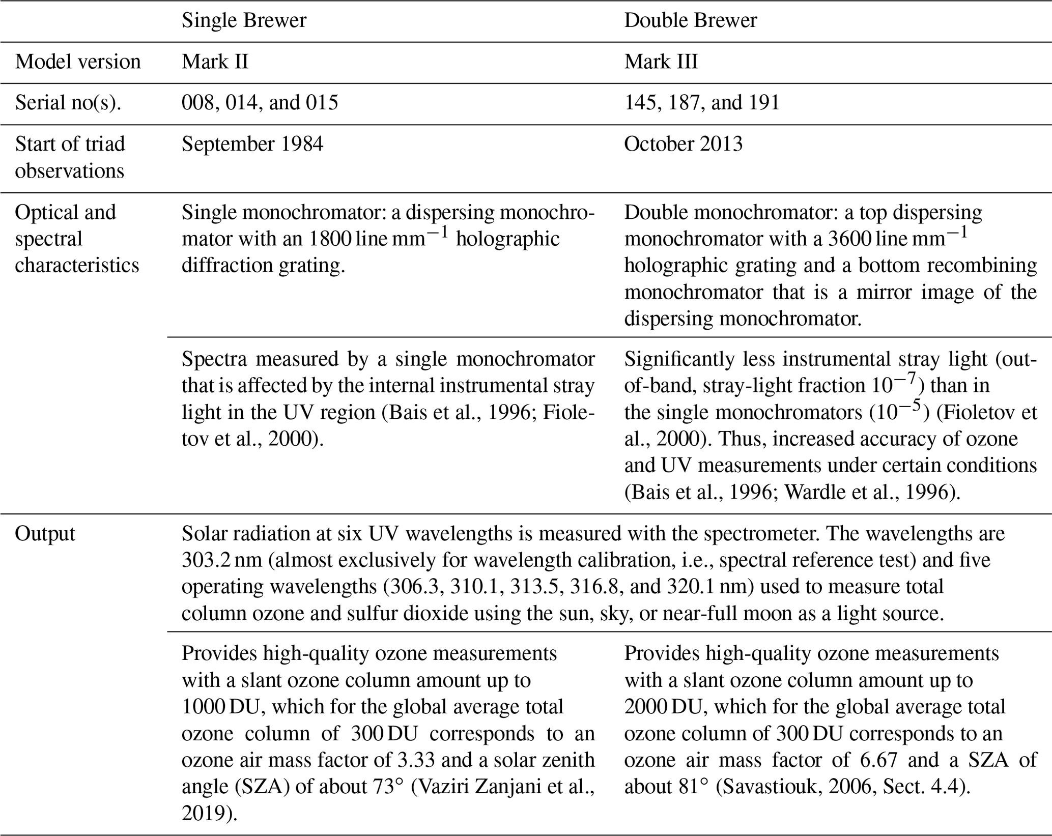
Table 1Specific features of single- and double-Brewer reference triads.
Previously, the assessment for the BrT, carried out by Fioletov et al. (2005), examined its 20-year-long record of direct-sun (DS) total ozone measurements (1984–2004). It was found that the BrT's precision over these two decades was better than ±1 % (Fioletov et al., 2005). There is no further published assessment for the world reference instruments after that period and no formal assessment made for the BrT-D yet. In addition, with the increasing number of satellite observations (e.g., OMI, TROPOMI) and ground-based observations from emerging technologies (e.g., Pandora spectrometer) of total ozone columns, it is important to compare the triad datasets with these measurements.
This paper provides a more recent assessment for the BrT (1999–2019) and reports the first assessment of the BrT-D (2013–2019). It is organized as follows: Section 2 describes the ground-based ozone measurements, satellite ozone measurements, and the model reanalysis ozone data. In Sect. 3, the standard and the new evaluation schemes are introduced, with a detailed description of a new third-party evaluation model. In Sect. 4, the world Brewer reference instruments' (BrT and BrT-D) data products are evaluated by the standard and new schemes. Lastly, Sect. 5 discusses the challenges for Brewer instruments to measure ozone at a level better than 1 %, in the context of the comparison between the world reference triads, regional triads, and high-resolution satellite data. Conclusions are given in Sect. 6.
2.1 Brewer
There are several model versions of the Brewer instrument. The Mark I prototype instruments were tested and operated since the 1970s (Kerr et al., 1981). The first production version (Mark II) was introduced in the early 1980s. In the 1990s, the double monochromator (Mark III) was developed to reduce the internal instrumental stray light, which allows high-quality total column ozone measurements in large slant column ozone (e.g., low sun elevation) conditions. There were other versions of Brewers developed in the late 1990s (i.e., Mark IV and V) to extend the measuring wavelengths and to measure other trace gases. Today, only the Mark III version of the Brewer instrument is manufactured. Table 1 summarizes some of the specific similarities and differences between the single- and the double-Brewer reference triads. More details about Mark II and III's measurement standard deviations and stray-light characteristics are provided in Appendix A.
The Brewer spectrophotometer provides data products that include column ozone (e.g., Kerr, 2002; Kerr et al., 1981), column sulfur dioxide (SO2; e.g., Fioletov et al., 1998; Zerefos et al., 2017), column nitrogen dioxide (NO2, by Mark IV only; e.g., Cede et al., 2006; Kerr et al., 1988), spectral UV radiation (e.g., Bais et al., 1996; Fioletov et al., 2002), aerosol optical depth (e.g., Kazadzis et al., 2005; Marenco et al., 2002), and effective ozone layer temperature (Kerr, 2002). However, the main data product provided by the Brewer instrument is the total column ozone via direct-sun observations. In this work, we focus on the Brewer direct-sun total column ozone data product only, although total column ozone also can be retrieved using solar zenith-sky radiance, solar global spectral UV irradiance, and lunar direct irradiance (Fioletov et al., 2011; Kerr, 2010). Brewer data were processed by Brewer Processing Software (BPS) developed by ECCC (Fioletov and Ogyu, 2008). The same processing software was used in Fioletov et al. (2005). The software demonstrated good performance in a recent comparison of available processing software tools for Brewer total ozone retrievals (Siani et al., 2018).
The Brewer spectrophotometer is a modified Ebert grating spectrometer that was designed to measure almost simultaneously the intensity of radiation at six selected channels in the UV (nominally 303.2, 306.3, 310.1, 313.5, 316.8, and 320.1 nm). The first channel is almost exclusively used for wavelength calibration. The four longer wavelengths are used for the total column ozone (Ω) retrieval via the following equation:
where m and μ are the enhancement factors for the slant pathlength of the direct radiation relative to vertical path for air and the ozone layer respectively (also known as the air mass factors). F, Δα, and Δβ are the linear combinations of the logarithms of the measured intensity (base 10), the effective ozone absorption, and the Rayleigh scattering coefficients, respectively. For example, , where I3 to I6 are the photon count rates at channel number three to number six. F0 is the instrument response (F) if there were no atmosphere between the instrument and the sun; it is also known as the ETC. Details about the standard Brewer ozone retrieval algorithm can be found in Kerr (2010) and the references cited there. In the standard Brewer algorithm, Δβ, m, and μ are determined and pre-calculated and are not instrument-dependent. F0 and Δα (calibration constants) are unique for each instrument and depend on the exact wavelengths and band passes of the slits of each instrument (Kerr et al., 1985). After laboratory and field calibration (to determine Δα and F0, respectively), Ω is then readily calculated for each field observation (i.e., F).
As previously described, to maintain high-quality data of all Brewer instruments (i.e., transfer the F0 value), the world reference instruments (BrT and BrT-D) receive their F0 values via the independent calibration technique. In short, these high-precision F0 values were determined by fitting the measured F values as a linear function of air mass factor (see Eq. 1). For example, in clear-sky conditions with stable ozone values, if measurements are made under a range of air mass factors throughout a day, then the intercept of the linear fitting of (F+Δβm) versus μ will be F0. More technical details, such as calibration periods, averaging, and why MLO is the ideal site for this practice are provided in details in Kerr (2010). These values are transferred to the travelling standard and then to the field Brewers via co-located field calibration routines (i.e., calibration transfer method). The primary calibration history of the world Brewer reference instruments is summarized in Table 2. Due to building roof work at the Toronto site, the BrT-D was temporarily moved to Egbert, Canada (44.230∘ N, −79.780∘ W), at the beginning of September 2018 and deployed on the roof of the ECCC Centre for Atmospheric Research Experiments building (CARE, 251 m a.s.l.). The CARE building is located in a rural area, which is surrounded by farmlands. For this period between September 2018 and December 2019, the BrT-D was located about 55 km north-west from the BrT. This period of data is still used in the analysis to study and illustrate some fine-scale variations in the ozone field. More details about reference instruments' repair and upgrade review are provided in the Supplement.
Table 2Independent calibration history of world Brewer reference instruments.
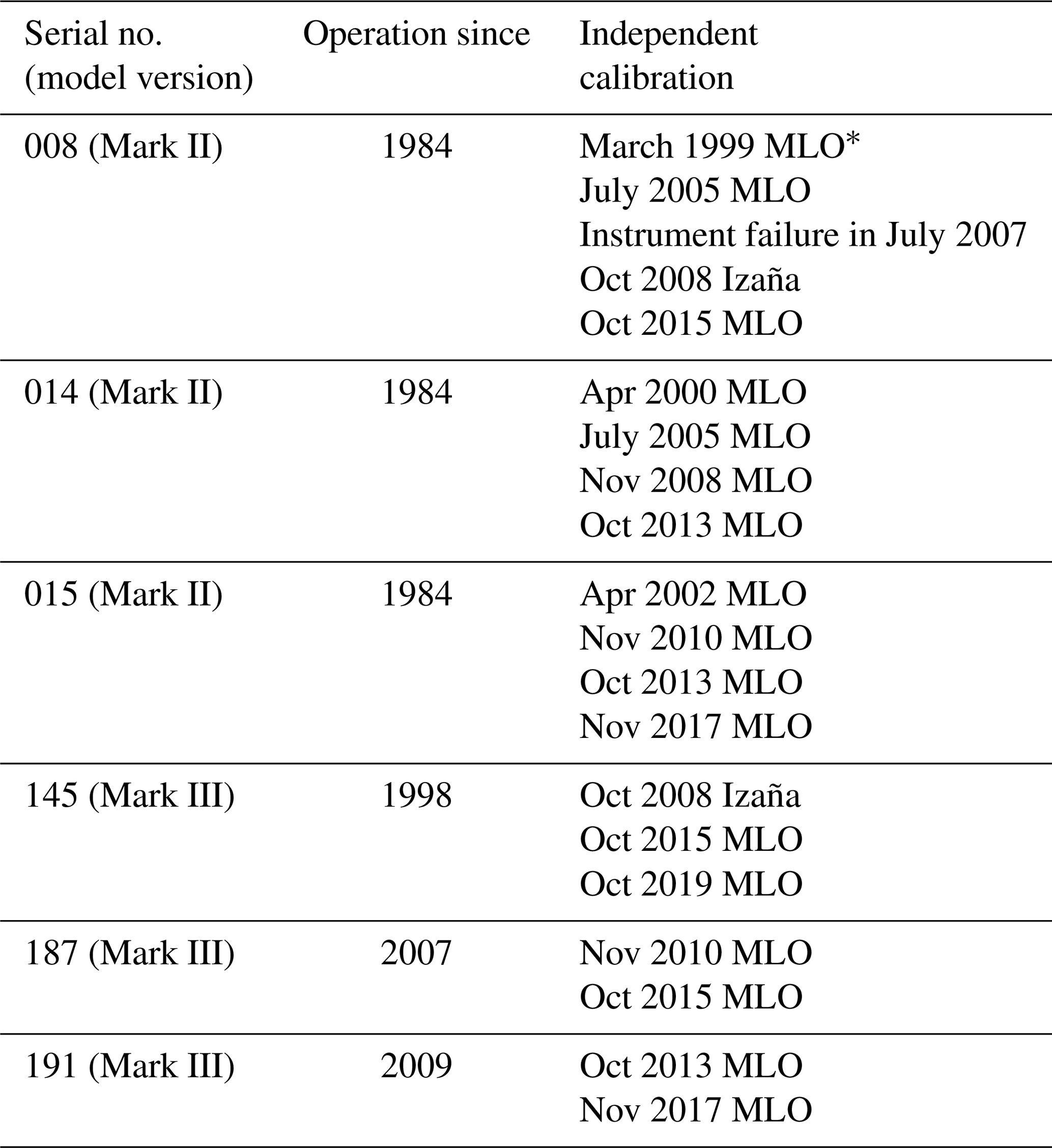
* MLO: Mauna Loa Observatory.
2.2 Pandora
The Pandora instrument records spectra between 280 and 530 nm with a resolution of 0.6 nm (Herman et al., 2009, 2015; Tzortziou et al., 2012). It uses a temperature-stabilized Czerny–Turner spectrometer with a 2048 × 64 pixels CCD detector. The spectra are analyzed using the total optical absorption spectroscopy (TOAS) technique (Cede, 2019), in which absorption cross sections for multiple atmospheric absorbers such as ozone, NO2, and SO2 are fitted to the spectra. Different from the Brewer instrument, which only uses intensities measured at four wavelengths, the Pandora instruments use the entire spectrum from 310 to 330 nm (at 0.6 nm resolution, with more than 160 pixels) in their ozone retrieval. The current Pandora standard ozone column retrieval algorithm uses a literature reference spectrum (composite of Kurucz, 2005, Thuillier et al., 2004, van Hoosier, 1996 and Gueymard, 2004, details in Cede, 2019) and does not retrieve the effective ozone temperature. Thus, Pandora standard ozone data products have a temperature dependence (Herman et al., 2015), i.e., 0.25 % K−1, when compared to Brewer measurements (Zhao et al., 2016). This temperature dependence introduces a 1 % to 3 % seasonal bias between the Pandora and the Brewer standard data products. Another major difference between the Brewer and Pandora retrieval algorithms is their selection of an ozone cross section; i.e., the Brewer instrument uses the BP (Bass–Paur) ozone cross section (at 228.3∘ K, Bass and Paur, 1985), and the Pandora instrument uses the Serdyuchenko ozone cross section (at 225∘ K, Serdyuchenko et al., 2014). As a result of temperature dependency and different selection of ozone cross sections, a two percentage multiplicative bias between the Pandora and Brewer standard ozone column products was found in Zhao et al. (2016). Thus, in this work, the Pandora ozone data are corrected by an empirical method with the ozone-weighted effective temperature (Zhao et al., 2016). The effective temperature was calculated from temperature and ozone profiles provided by ERA-Interim (Dee et al., 2011). In general, after correction, the multiplicative bias in Pandora ozone data can be decreased from 2.92 to −0.04 %, with the seasonal difference (estimated with monthly data) decreased from ±1.02 % to ±0.25 % (see Fig. 11 in Zhao et al., 2016; i.e., comparing to Brewer, corrected Pandora data have % offset in summer and offset in winter). An effective ozone temperature retrieval algorithm is under development for the Pandora instrument to minimize its temperature dependence effect (Cede, 2019). Additional information on Pandora calibrations, operation, retrieval algorithms, and the correction method can be found in Cede (2019; Cede et al., 2019), Tzortziou et al. (2012), and Zhao et al. (2016).
Pandora instrument no. 103 has been making direct-sun measurements in Toronto (co-located with BrT and BrT-D) since 2013 (Zhao et al., 2016). The instrument has made almost daily measurements since its deployment, except during a filter upgrade in 2017. The 7 years of data (2013–2019) have been reprocessed and harmonized by the Pandonia Global Network (PGN) to ensure the high quality of its ozone data product. In this work, only high-quality Pandora ozone data products are used (Pandora level 2 (L2) data product quality flag = 0; Cede, 2019). Originally, Pandora no. 103 was operated in DS mode only, and Pandora DS ozone data had a 1 min resolution. Starting in 2018, it was operated in the combination mode (i.e., direct-sun, zenith-sky, and multi-axis) and Pandora DS ozone data had a 5 min resolution. The Pandora and BrT-D instruments have good stray-light control, under typical ozone conditions (i.e., slant column ozone less than 1500 DU), and their air mass dependence is comparably low up to 81.6∘ SZA (within 1 % up to AMF = 5.5; Zhao et al., 2016). Benefitting from the TOAS technique, unlike Brewers, Pandora instruments do not need the independent calibration at MLO (Tzortziou et al., 2012).
2.3 Satellites
The BrT's performance was evaluated against the Total Ozone Mapping Spectrometer (TOMS) and reported in Fioletov et al. (2005). With more satellite instruments reporting total ozone columns, here we present a data comparison between the Brewer reference instruments (BrT and BrT-D) and multiple satellites, including TOMS, NOAA Solar Backscatter Ultraviolet Radiometer 2 (SBUV) series (nos. 11, 14, 16, 17, 18, 19), Ozone Mapping and Profiler Suite (OMPS), Ozone Monitoring Instrument (OMI), and TROPOspheric Monitoring Instrument (TROPOMI).
2.3.1 TOMS
There were four TOMS in orbit: on the Nimbus-7 satellite launched in 1978, on Meteor-3 in 1991, and on ADEOS and Earth Probe (EP) in 1996. Total column ozone was derived from incident solar radiation and backscattered ultraviolet sunlight measurements. TOMS total column ozone has been widely used for verification of ground-based measurements (e.g., Fioletov et al., 1999; Kyrö, 1993). Fioletov et al. (1999) reported that about 80 % of the Dobson and Brewer data have standard deviations of monthly mean difference with TOMS that are less than 2.5 %. The TOMS-EP total ozone data from 1996 to 2005 with a quality flag of zero were used in this work (McPeters et al., 1998).
2.3.2 SBUV series
Total column ozone from the NOAA SBUV series (nos. 11, 14, 16, 17, 18, 19) is used in this work. Unlike TOMS, OMI, or TROPOMI, which provides daily global coverage, the non-scanning, nadir-viewing SBUV instruments provide full global coverage approximately biweekly. The SBUV ozone column data used in this work are produced and quality assured by the overpass algorithm to create daily overpass values (Labow et al., 2013; by weighted-interpolating data measured within the box centred on the station location (±2∘ in latitude and ±20∘ degrees in longitude)). Labow et al. (2013) reported that the total column ozone data from Brewers and SBUVs show an agreement within ±1 % over 40 years (1970–2010; yearly relative difference).
2.3.3 OMPS Nadir Mapper
The OMPS on the Suomi National Polar-orbiting Partnership (Suomi NPP) satellite was launched in 2011 (Flynn et al., 2014; Kramarova et al., 2014). OMPS includes nadir and limb modules to measure both profile and total column ozone concentrations. In this work, OMPS-NPP L2 Nadir Mapper (NM) total column ozone swath orbital v2.1 data (only the good sample, with a quality flag of zero) from the OMPS-NM module is used. Flynn et al. (2014) reported that the OMPS column ozone (from an earlier v1) has a bias with other records (e.g., OMTO3) on the order of −3 %.
2.3.4 OMI
The OMI instrument on the Earth Observing System Aura satellite was launched in 2004. OMI has two standard data products, OMDOAO3 (Veefkind et al., 2006) and OMTO3 (Bhartia and Wellemeyer, 2002), which are produced using differential optical absorption spectroscopy (DOAS) and TOMS-like techniques, respectively. The mean difference between the two data products varies from 0 to 9 DU (0 %–3 %) with latitude and season (Kroon et al., 2008). In this work, the OMDOAO3 and OMTO3 overpass (OVP) data are used, with the L2 quality flag equal to 0 or 1 (and bit 6 not set) included (see https://avdc.gsfc.nasa.gov/pub/data/satellite/Aura/OMI/V03/L2OVP/OMDOAO3/, last access: 10 March 2020).
2.3.5 TROPOMI
TROPOMI, on board the Copernicus Sentinel-5 Precursor satellite, was launched in 2017. The offline (OFFL v010107) total ozone column data (Garane et al., 2019) are used in this work (only L2 data with qa_value ≥0.75 are included). Garane et al. (2019) reported that the mean bias and the mean standard deviation of the percentage difference between TROPOMI and Brewer ground-based total ozone column data are within 1 % and 2.5 %, respectively.
2.4 MERRA-2 reanalysis data
The second Modern-Era Retrospective analysis for Research and Applications (MERRA-2) is an atmospheric reanalysis from NASA's Global Modeling and Assimilation Office (GMAO). MERRA-2 assimilates partial total column ozone retrievals from the SBUV series from 1980 to 2004. From October 2004, MERRA-2 assimilates ozone profiles and total column data from the Microwave Limb Sounder (MLS) and the OMI, respectively (Wargan et al., 2017). MERRA-2 column ozone data have been found to be of good quality when compared with satellite and ground-based observations (e.g., Rienecker et al., 2011; Wargan et al., 2017; Zhao et al., 2017, 2019). In this work, the MERRA-2 total column ozone (0.5∘ × 0.625∘, version 5.12.4) with 1 h temporal resolution is used as an input in the third-party comparison model (see Sect. 4 for more details).
Multiple Brewer instruments at the same site may not measure ozone at exactly the same time. To compare the ozone column data provided by each Brewer reference instrument, a baseline ozone column value at the time of each measurement should be established. Ideally, if the true ozone column values are known, then the performance of each instrument can be evaluated as simple as calculating the discrepancies between true ozone and measured ozone. However, this approach is not possible in reality. Several other means to form these (daily or time-resolved) baseline ozone values were used in the past: (1) the average of all satisfactory measurements for each instrument (Kerr et al., 1998), (2) a second-order time-resolved statistical model (Fioletov et al., 2005), (3) a third-order simple polynomial fit (Stübi et al., 2017b), and (4) a fourth-order time-resolved statistical model (León-Luis et al., 2018). In general, these approaches aim to define the best baseline total column ozone values for each day, which are as close to true ozone values as possible. Apparently, the first method (i.e., simple daily mean) is not ideal since it includes the effects of ozone changes during the day combined with differences in the timing and number of measurements by each instrument (Fioletov et al., 2005), and instrument uncertainties are overestimated. The second method takes the daily baseline ozone values as a second-order function, which are fitted using all satisfactory measurements for all three instruments together but also give the individual instrument a degree of freedom in offsets. The third method takes the ozone changes into account, but it is still affected by the number of measurements from each instrument (i.e., the instrument reporting more data points will dominate the baseline). The advantage of the time-resolved model (second or fourth method) is that it takes both effects of ozone changes into account and minimizing the impact of sampling (i.e., all three instruments share the same first- and second-order terms, while the offset terms are unique for each instrument; see more details in the following section). It should also be noted that third- or higher-degree polynomial fit does not really change the results much because the baseline is only needed to adjust for the time difference in ozone measurements by individual Brewers. Thus, to make the current work directly comparable to previously reported results for the world reference instruments, we only use the second approach in the analysis (i.e., second-order time-resolved statistical model; following Fioletov et al., 2005, referred to as Model 1).
In addition to constructing the baseline with the individual Brewers' data, we can use third-party (e.g., co-located, independent total column ozone measurements from Pandora) measurements as the baseline ozone in the evaluation. The Pandora instrument typically has a better temporal resolution than Brewers and, therefore, can capture most of the daily ozone variations better. Moreover, when using coincident Pandora ozone data, the baseline will not have the sampling or weighting issues; i.e., the Brewer instrument that reported more data points will not dominate the forming of the baseline (i.e., as the baseline formation in Model 1; see Eq. 2). However, when using this third-party baseline, we should be cautious about the difference between Pandora and Brewer ozone data products, i.e., their seasonal and multiplicative bias. Details about how to interpret the third-party assessment results are provided in Sect. 4.
3.1 Comparison with ground-based instruments
3.1.1 The original method
Two statistical models have been developed to evaluate Brewer reference instruments' performance by Fioletov et al. (2005). The first model is a time-resolved second-order model (referred to as Model 1) to provide the baseline ozone and applied to the reference triad data from each day:
where Ω is an ozone measurement from one of the three Brewers (e.g., BrT, or here with arbitrary serial nos. 1, 2, and 3), t is the corresponding time of the measurement, and t0 is the local solar noon time. The I1, I2, and I3 are the indicator functions for each of the three Brewers. For example, if the ozone value Ω is measured by Brewer no. 1, I1 is set to 1 (and set to 0 for the two other Brewers). The coefficients A1, A2, A3, B, and C can then be estimated by the least-squares method. Please note here that the ozone values for this day are then represented by three second-order curves, which share the common curvatures (B and C terms) but have a different offset (i.e., A1, A2, and A3). In other words, each instrument formed its own daily time-resolved ozone variations, but these variations are not totally independent from each other (since they share the B and C terms). Then, the average of the three coefficients is used as the benchmark to evaluate the performance of individual instruments. For example, (A1−A) represents the deviation of Brewer no. 1 from the baseline ozone (i.e., corresponding to -t0)+ C(t-t0)2).
In general, with contributions from all three instruments, this model removes the diurnal ozone variations relative to the noon ozone value. Meanwhile, the model preserves the instrumental differences as much as possible by assigning different offsets for each baseline (i.e., corresponding to an assumption that there is only an additive bias between Brewers).
For a well-calibrated and well-maintained Brewer instrument, its major uncertainties in derived ozone column data came from two instrument constants assigned to it (i.e, F0 and Δα). Next, to further break down the uncertainty budgets, Model 2 is designed by combing Eqs. (1) and (2) as
where and Δα′ are the assigned ETC and effective ozone absorption coefficient values. X and Y are the assigned uncertainties to these two instrument constants. Here, the total column ozone amount (Ω) is replaced by the Model 1 defined baseline ozone. Next, X and Y can be estimated for each of the three instruments using the least-squares method for each 3-month season. In general, Model 2 assumes that the baseline ozone provided by Model 1 is the ground truth (i.e., true ozone values). Thus, the difference of total column ozone between the individual instrument and Model 1 is allocated to the error of ETC and effective ozone absorption values. As the stray-light issue in high-μ conditions may affect the formation of the baseline ozone (see Eqs. 2 and 3), all Brewer DS ozone data used in this study have μ≤3.5.
3.1.2 Third-party scheme
The design of Model 2 is based on our assumption of the high quality of Brewer ozone data, i.e., the Brewer-derived baseline ozone (Model 1 ozone) is close to the true ozone. In general, for well-calibrated and well-maintained Brewer instruments, this assumption is valid. For example, if Brewer nos. 1 and 2 are in good condition but Brewer no. 3 is not, Model 1 will show the discrepancy. Then, we can easily identify the issue and re-calibrate Brewer no. 3. However, if Brewer nos. 1 and 2 are the instruments with larger discrepancies from true ozone and Brewer no. 3 is in good condition, then things will become more complex. In addition, whenever we select three instruments to form a triad and use models 1 and 2 to perform the analysis, we also selected the baseline ozone defined by those three instruments. In other words, the Model 1 and 2 analyses applied to BrT and BrT-D cannot reflect their relative difference; i.e., BrT uses BrT's baseline, whereas BrT-D uses BrT-D's baseline. Thus, to better evaluate and compare BrT and BrT-D's performances, we need to use a third-party ozone column data as the baseline. Here, Model 3 is designed as
where the only difference compared to Model 2 is that we replaced the Model 1 defined baseline ozone with a new third-party baseline ozone (Ω3rd-party). The new baseline can be supplied by either other co-located and independent ozone column observations (e.g., Pandora ozone data) or reanalysis data (e.g., MERRA-2). Please note here the Ω3rd-party has to be independent of Brewer reference instruments. For example, they cannot be measurements from another Brewer (e.g., another co-located field Brewer instrument) unless it received its ETC constant via the independent calibration method.
When a third-party baseline ozone exists, it is easy to evaluate the deviation of each Brewer from the baseline ozone. Thus, in this work, when using the third-party baseline ozone, we simply report their absolute and relative differences defined as
3.2 Comparison with satellites
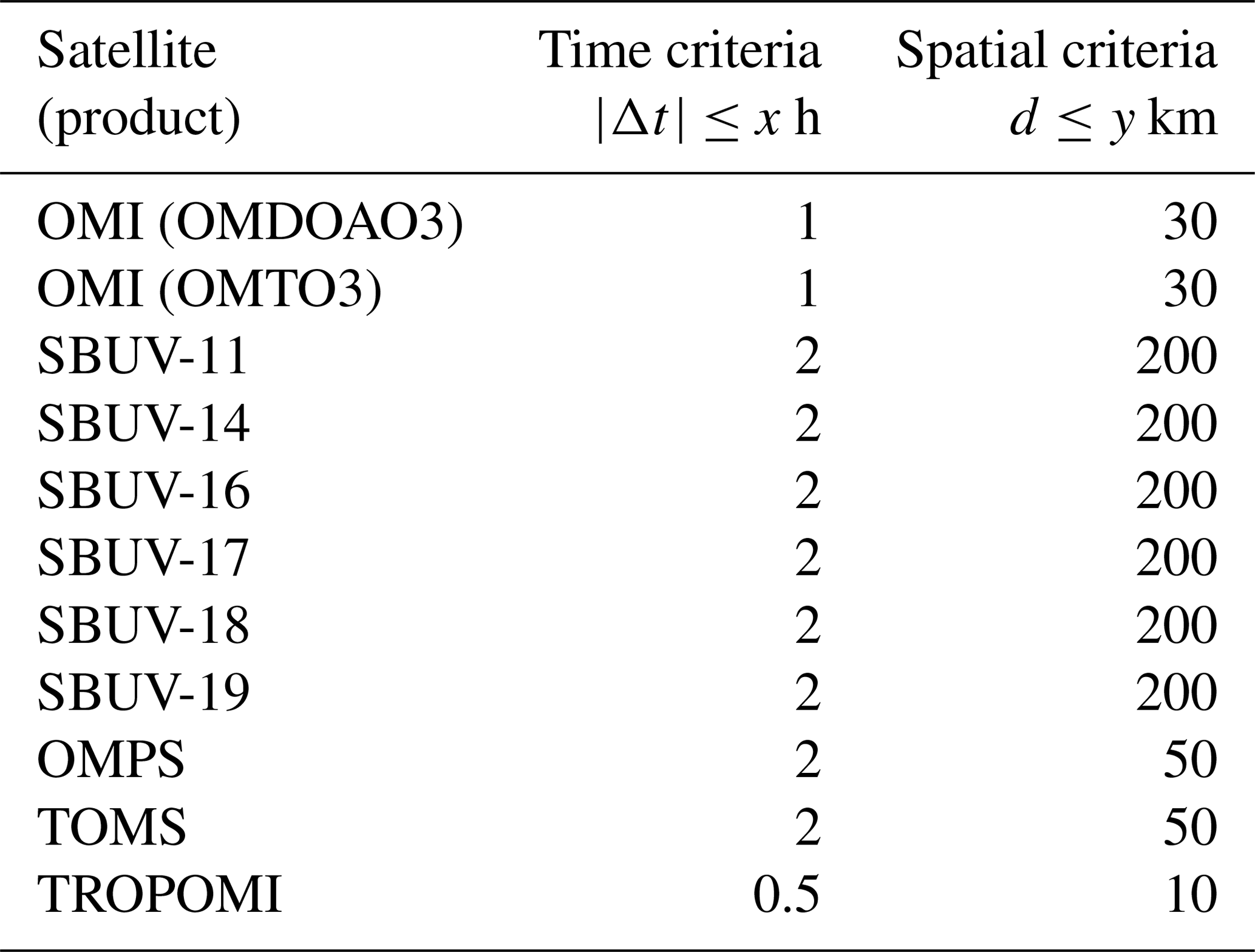
Regression analyses between Brewer and satellite observations were made by using the following coincident criteria: (1) nearest (in time) measurement that was within ±x h of satellite overpass time and (2) closest satellite ground pixel (having a distance (d, in km) from the ground pixel centre to the location of the Brewer instruments less than y km). These coincident criteria are summarized in Table 3. Only good quality satellite data are used in the analysis. For example, OMTO3 with only an error flag equal to 0 (good sample) are used.
The assessment of the Brewer reference instruments was performed using models 1, 2, and 3 defined in Sect. 3. The time series of Brewer reference triads' total column ozone (TCO) observations in Toronto is shown in Fig. 1. To ensure the assessment is based on good quality data, the data were strictly filtered (i.e., data from single- and double-spectrometer instruments with reported standard deviation >3 DU or μ>3.5 are removed). Using 3 DU (Fioletov et al., 2005) instead of the standard 2.5 DU (Fioletov and Ogyu, 2008) yields more data points and, therefore, more days suitable for comparison but does not improve the comparison since the additional measurements are the noisiest.

Figure 1Time series of Brewer reference triads' total column ozone observations in Toronto. Vertical black dash lines indicate the time of primary calibrations as shown in Table 2.
4.1 Comparison of ground-based instruments
4.1.1 Model 1
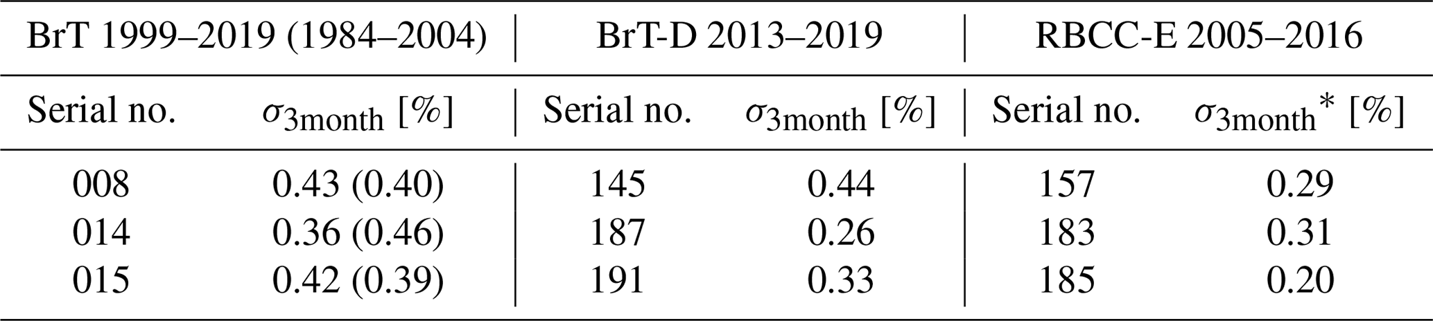
To perform Model 1 analysis, additional criteria are applied. A specific day is analyzed with Model 1 only if each of the three instruments has (1) at least 10 measurements on that day and (2) at least three measurements in each half-day (defined by local solar noon time) on that day. The Model 1 analysis was done for BrT and BrT-D separately. The deviations of each individual instrument from their baseline are shown in Fig. 2a, which are comparable to the results in Fig. 1 from Fioletov et al. (2005). The residuals from Model 1 include some remaining instrument uncertainties but also some short-term fluctuations in ozone, which are not reflected by the second-degree polynomial model. The uncertainties include the effects of instrument temperature fluctuations and the differences in the characteristics of the neutral density (ND) filters. The 5th and 95th percentiles of the Model 1 residuals are shown in Fig. 2b, which are comparable to the results in Fig. 2 from Fioletov et al. (2005). The standard deviation of the residuals is about 2.4 DU or 0.72 %. In general, these updated results show that the performance of the BrT in the last two decades (1999–2019) is comparable to its reported values from 1984 to 2004. The long-term instrument drifts are still typically within ±1 %. Using the analytical method from the first assessment work (Fioletov et al., 2005), the deviations and residuals are reported with frequencies of 3 months and 1 year, respectively, in Fig. 2. These frequencies were used because they provide a good balance between sampling frequency and sufficient co-incident measurements as well as preserve a potential seasonal component in the differences. The standard deviations (σ) of the 3-month averages plotted in Fig. 2a are 0.43 %, 0.36 %, and 0.42 % ( %) for Brewers no. 008, no. 014, and no. 015, which are comparable to the reported values from 1984 to 2004 (0.40 %, 0.46 %, and 0.39 %). The double triad also shows good long-term stability with the Model 1 analysis, where all measurements are within ±1 % compared to its baseline. The standard deviations are 0.44 %, 0.26 %, and 0.33 % ( %) for Brewers. no. 145, no. 187, and no. 191. From this, assuming that the instrument uncertainties are independent, the standard uncertainty of Brewers (δ) can be estimated as , i.e., 0.49 % and 0.42 % for BrT and BrT-D, respectively.
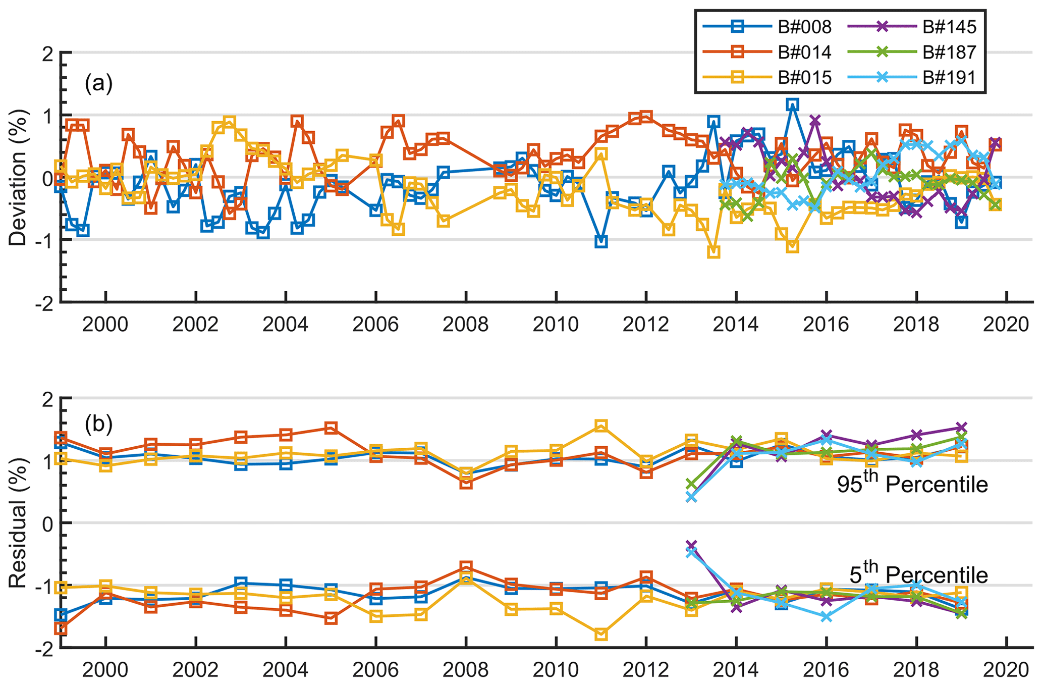
Figure 2Model 1 estimated deviations and residual of ozone values. (a) Deviations of ozone values of individual triad Brewers from the mean of the three instruments. Each point on panel (a) represents a 3-month average. Panel (b) shows the 5th and 95th percentiles of the residuals of the Model 1 analysis. Each point on panel (b) is based on 1 year of data.
4.1.2 Model 2
The Model 2 analysis was performed for BrT and BrT-D. Figure 3 corresponds to Fig. 4 in Fioletov et al. (2005). In general, Fig. 3 shows the errors in the ETCs, and effective ozone absorption coefficients account for up to ±2 % of total column ozone, as indicated in Fioletov et al. (2005). Here, the errors in the ETCs and effective ozone absorption coefficients are estimated in R6 ratio units (the units used in the actual Brewer processing algorithm; R6 values corresponding to measured slant column, i.e., in DU; ETCO). The errors are converted from R6 ratio units to percentages of total column ozone by using typical conditions for Brewer measurements in Toronto (i.e., Ω=330 DU, Δα=0.34, and μ=2) to provide more straightforward values to assess the impact of errors in the ETCs and effective ozone absorption coefficients. For example, if we have a model-estimated error of ETCO3 as 50 R6 ratio unit, it will correspond to % of total column ozone using the typical conditions described above. In typical conditions, the uncertainties of ozone absorption coefficient are within ±1 micrometer step based on the dispersion test, which corresponds to approximately ±0.3 % of total column ozone. For the uncertainties of ETC, the goal is to have it within ±5 R6 ratio units.
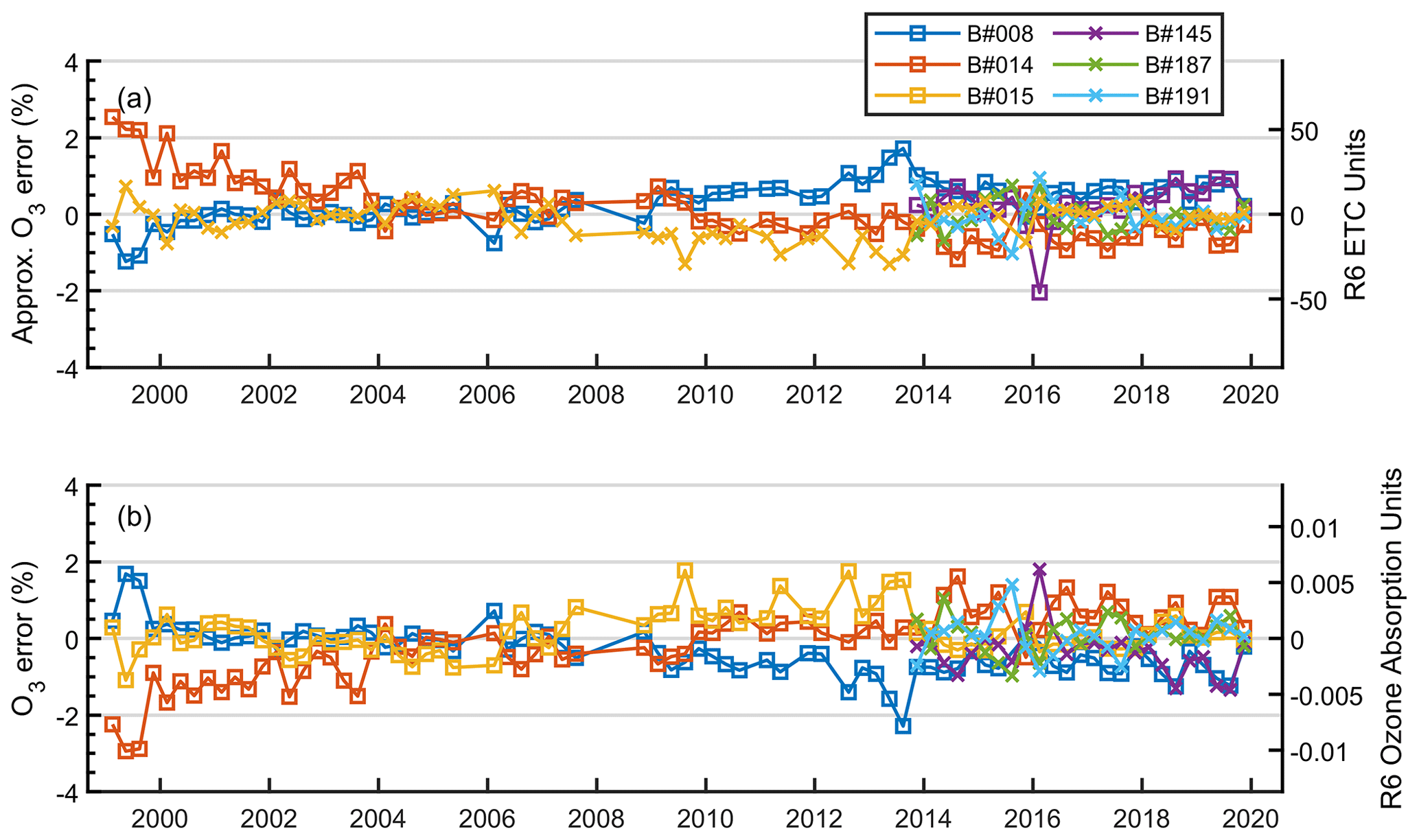
Figure 3Relative systematic uncertainties in ETCs and effective ozone absorption coefficients estimated using Model 2. The right y axes represent the values in the units used in the actual Brewer algorithm (i.e., R6 ratio units); the left y axes demonstrate the percent values of these errors in total ozone values. Each point on the graph represents a 3-month average.
The large errors in ETCs and ozone absorption coefficients may largely compensate for each other and not be evident in the Model 1 analysis. This is because Model 2 distributes the residuals (mismatch between observed ozone and baseline ozone) into two parts, i.e., X and Y terms in Eq. (3), which made the retrieved errors negatively correlated. For example, during 2013, there were significant errors in the assigned ETCs and absorption coefficients to no. 008 that were truly caused by wavelength range limitations of this early model Brewer. A measurement type was added to the schedule of this instrument, which when run reached the extent of physical travel of the micrometer causing a 2 nm shift in the measurement from the forward to the backward scan of the micrometer. The Model 2 results show that the BrT-D has had a similar performance compared to the BrT since 2013. The errors in ETCs and ozone absorption coefficients from BrT-D (within ±1 %) are even smaller than those from BrT in the most recent period (2017–2019).
4.1.3 Model 3
For a third-party-based ozone analysis (Model 3), Brewer and Pandora data are both averaged into 10 min bins and then paired. Note that the Pandora instrument sampling frequencies were reduced from one measurement every 1.5 min in 2013–2017 to one measurement every 5 min in 2018–2019 due to a change in the observation schedules.
Differences between the Pandora observations and the measurements by individual Brewers are shown in Fig. 4. The gaps in the Pandora record are caused by an instrumental failure in winter 2014. The absolute differences between Brewer and Pandora data are within ±8 DU. They are slightly larger in wintertime due to the temperature dependency in Pandora ozone data (although empirical correction methods have been applied, the residual effect still exists, e.g., Fig. 13 in Zhao et al., 2016). Thus, when using Pandora data as a third-party baseline, it is more important to examine the variation of relative differences (i.e., Δrel of one Brewer minus Δrel of another Brewer). In the period of the example, the relative differences between Brewer no. 015 and Brewer no. 145 are within 5 DU. Thus, the Brewer instruments' performance was, in fact, stable in that period. Figure 4 shows the relative differences, indicating that, compared to Pandora, all Brewer reference instruments have long-term stability within ±2 %. This result is not as good as the prediction from Model 1 (which shows ±1 % deviations) because, even corrected, Pandora data still have some residual seasonal bias. For shorter periods (e.g., summer 2016), all six Brewers have a relative difference within the range from 0 to −2 %, which is comparable to a ±1 % when Brewer instruments themselves are used as baselines.
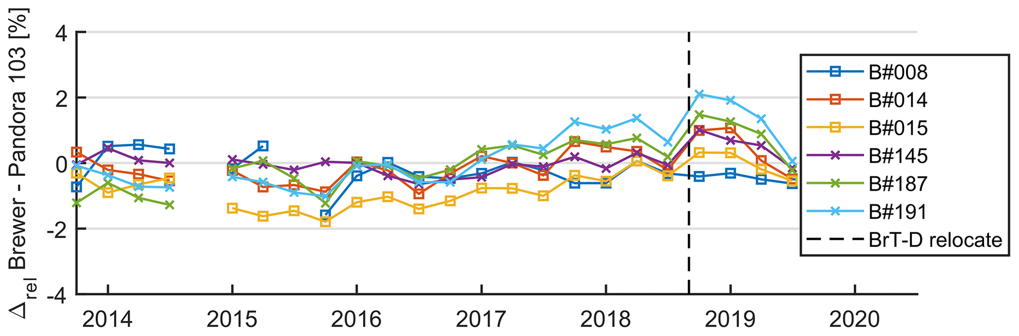
Figure 4Three-month relative differences between Brewers and Pandora total column ozone. Three-month averages are calculated if there are at least 10 coincident measurements between Brewer and Pandora for that period. The black dash line represents the time when BrT-D was relocated to Egbert; i.e., Pandora and BrT-D were not co-located.
We also can assess the performance of individual instruments from a third-party ozone baseline. For example, when compared to any other reference instruments, Brewer no. 015 gave the lowest ozone in the period from 2015 to 2017. Another example is the period after the BrT-D was relocated to Egbert, in which the discrepancy between BrT and BrT-D data became obvious (up to 4 % relative difference between Brewers no. 008 and no. 191).
The Model 3 analysis results are shown in Fig. 5, where the errors in ETCs and ozone absorption coefficients from each Brewer are reported independently. They show that the quality of these instrument constants can drift in time due to the nature of the calibration and maintenance work performed on the instruments. In general, Fig. 5 shows that in most cases, the estimated ETC and effective ozone absorption errors for all reference instruments are within ±2 %, i.e., similar to the Model 2 results (see Fig. 3).
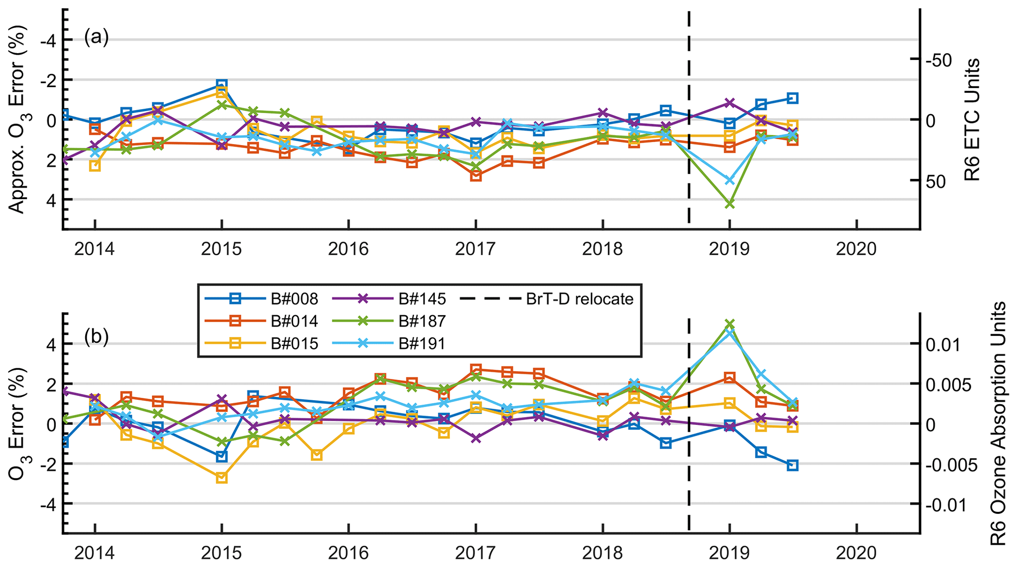
Figure 5Relative systematic uncertainties in ETCs and effective ozone absorption coefficients estimated using Model 3. Description of y axes is in Fig. 3. Each point on the graph represents a 3-month average. The black dash line represents the time when BrT-D was relocated to Egbert.
When compared to Model 2, Model 3 provides independent estimates of ETC and effective ozone absorption errors; i.e., errors for BrT and BrT-D can be compared directly. For example, in Fig. 3a, we cannot directly compare the ETC errors from Brewer no. 014 with those from Brewer no. 145 because they were evaluated by different baselines. However, with Fig. 5, we can conclude that Brewer no. 145 has about 1 % lower ETC errors than those for Brewer no. 014. The detailed results of ETC and ozone absorption coefficients errors are summarized in Table 4. In general, for this assessment period (2013–2019), Brewers no. 008, no. 015, and no. 145 have lower ETC and effective ozone absorption coefficients errors (within ±0.5 %) when compared to the other Brewer reference instruments.
Table 4(a) Mean errors of Δα and ETC for Brewer reference instruments (2013–2019) estimated with Model 3. (b) Mean errors of Δα and ETC for Brewer reference instruments estimated with Model 2.

1 Mean percent error in total column ozone, related to error in ozone absorptions. 2 Mean percent error in total column ozone, related to error in ETC, corresponding to X when μ=2, Δα=0.34, and Ω=330 DU (see Eq. 3).
As discussed in Sect. 4.1.2, sometimes Model 2 may also overlook issues if two out of three instruments have the compensation effect (i.e., errors in ETCs and ozone absorption coefficients compensate for each other). For example, when analyzing Brewer no. 145 data, it was revealed by the Model 3 analysis that its absorption coefficients were not ideal (in 2014; see Appendix B for more details). The issue was not observed with Model 2 due to Brewer no. 191 also having a similar issue in the same period. Thus, besides providing independent uncertainties, the Model 3 analysis can provide an important additional quality control process. Details about this additional quality control process are provided in Appendix B.
4.2 Comparison with satellite and reanalysis data
Eleven satellite overpass column ozone datasets are used for data verification of the Brewer reference instruments. Figure 6 shows the relative differences between satellite and Brewer measurements for seasonal (3 months) values are within ±4 % and yearly values are within ±3 % (not shown here) in these two decades (1999–2019). The standard deviation (σ3month) of the 3-month Brewer–satellite relative differences is 1.38 %. Detailed regression analysis was also performed, and some results are summarized in Fig. 7.
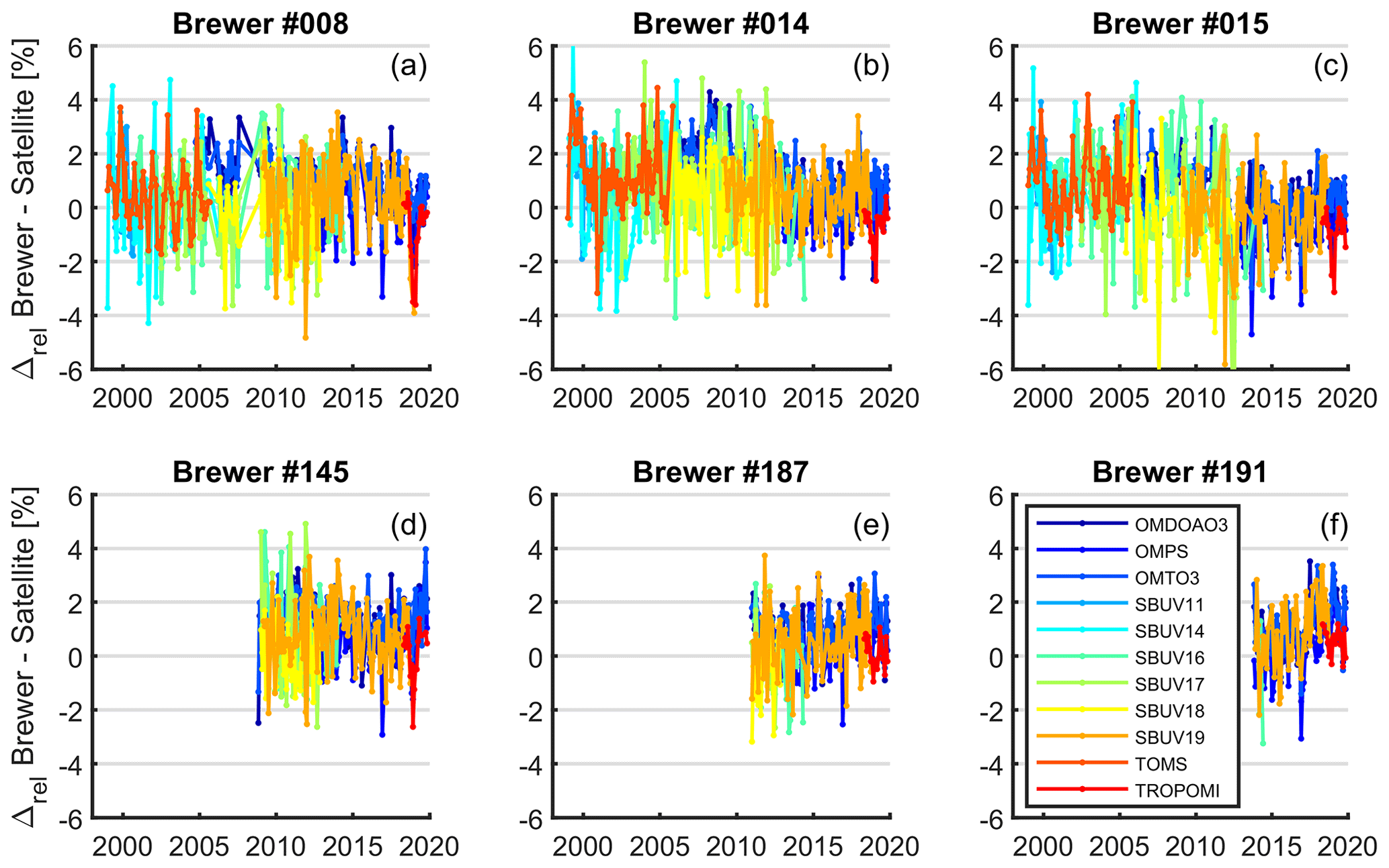
Figure 6The relative difference between satellites and the world Brewer reference triads (BrT and BrT-D). Each point represents a 3-month average. Brewers and satellite data are paired with the criteria shown in Table 3.
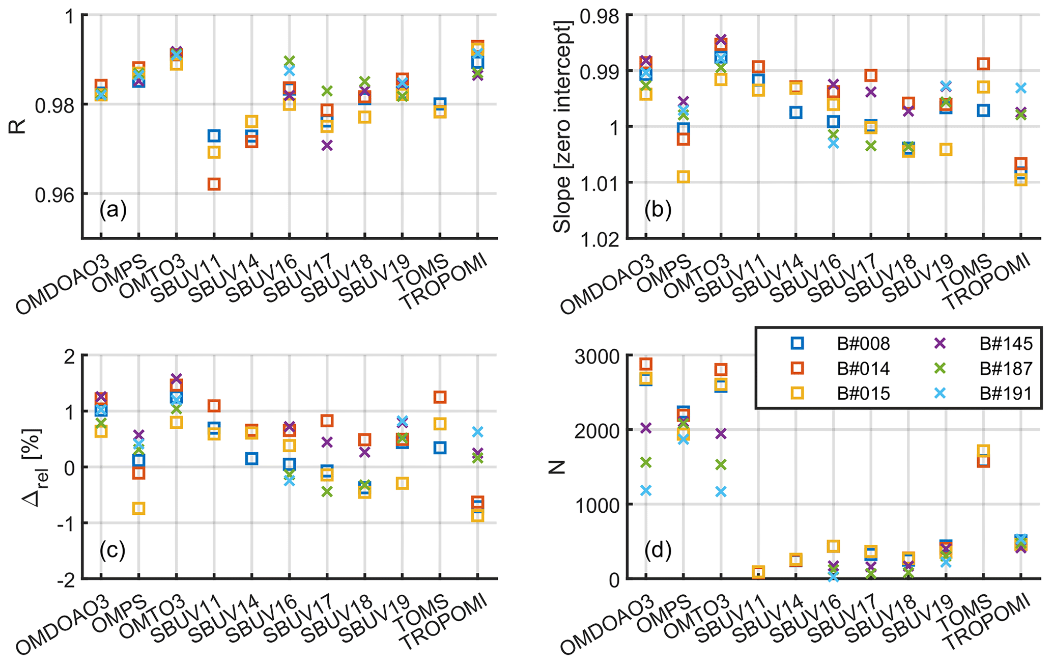
Figure 7Summary of the regression analysis between satellites and the world Brewer reference triads. The four panels represent the (a) correlation coefficient (R) between individual Brewer instruments and different satellites (labelled at the bottom axis), (b) the slope of the zero intercept regression line (multiplicative bias), (c) relative percentage difference (bias), and (d) the total number of coincident observations.
In general, the measurements from the individual Brewers have −1 % to 2 % relative difference when compared with all these 11 satellite datasets, with correlation coefficients >0.96. For most satellite datasets, the regression with zero intercept (Fig. 7b) also shows that the multiplicative biases between Brewers and satellites are well within ±1 %. It is known that satellite data also have some biases and drifts (e.g., Antón et al., 2009; Kroon et al., 2008); therefore, the Brewer–satellite difference values alone do not represent the Brewer instrument performance. Comparison with OMI (both versions) shows that besides the 1 % systematic difference between Brewers and satellite data, the spread of biases with individual instruments is also around 1 %. The standard deviation of the Brewer–OMTO3 (OMDOAO3) difference (for 3-month averages) calculated for six instruments is 0.99 % (1.06 %), about 0.5 % higher than Brewers' standard random uncertainties calculated in Sect. 4.1.1. It is also found that Brewers have lower relative differences compared with OMDOAO3 than OMTO3, which is in agreement with previous researches (e.g., Antón et al., 2009). For high-resolution satellites, such as TROPOMI, the interpretation of the results should be made with extra cautions as the line of sight of ground-based and satellite instruments should be accounted for (see more details in Sect. 6). In general, BrT and BrT-D's stabilities are assessed by using each satellite dataset, via the standard deviations of 3-month Brewer–satellite relative differences, as shown in Table 5. The results show that the BrT-D (σ3month=1.15 %) has a slightly better long-term stability than the BrT (σ3month=1.33 %), which is consistent with the results in Sect. 4.1.1 that BrT-D has lower random uncertainty than BrT.
Table 5Mean () and standard deviation (σ3month) of the 3-month Brewer–satellite relative differences.
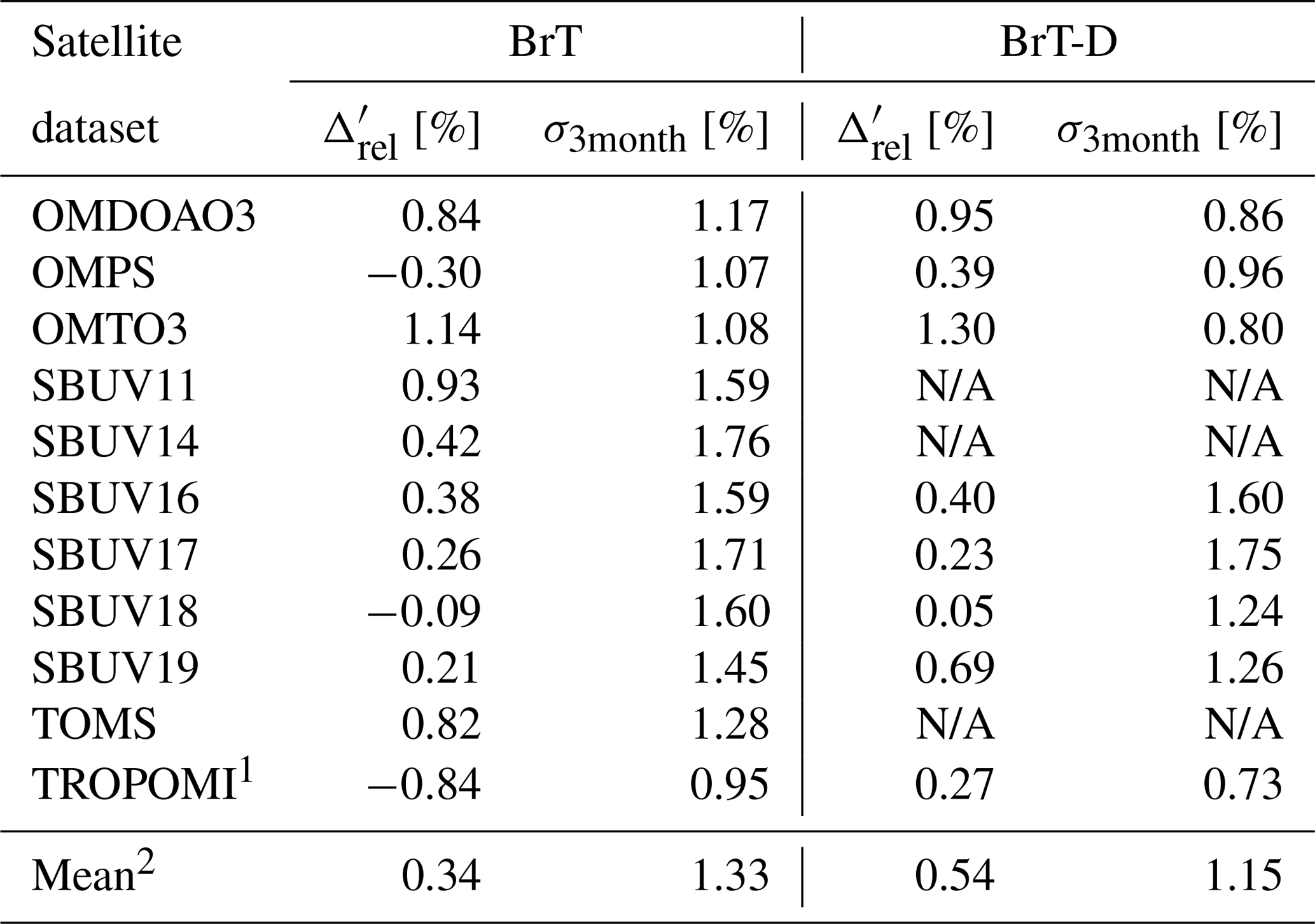
1 The comparison includes the period when BrT and BrT-D were not collocated (see Sect. 5 for more details). 2 Mean: only includes the satellite datasets that have overlap with both BrT and BrT-D. N/A: not applicable.
To compare with the hourly reanalysis data (MERRA-2 column ozone for Toronto), Brewer column ozone data were resampled to hourly mean values. The relative difference in time series is shown in Fig. 8, which demonstrated similar long-term stability (i.e., the relative difference within ±2 %) of the Brewer reference instruments when compared with Pandora or satellite instruments. For example, as in Fig. 4 (comparison with Pandora), Brewer no. 015 is found to have the lowest column ozone values from 2015 to 2018. In general, the relative differences between Brewers and the reanalysis datasets are within ±2 %. The inter-instrument differences (i.e., the differences between Brewers) are within ±1 % for most of the measurement period.
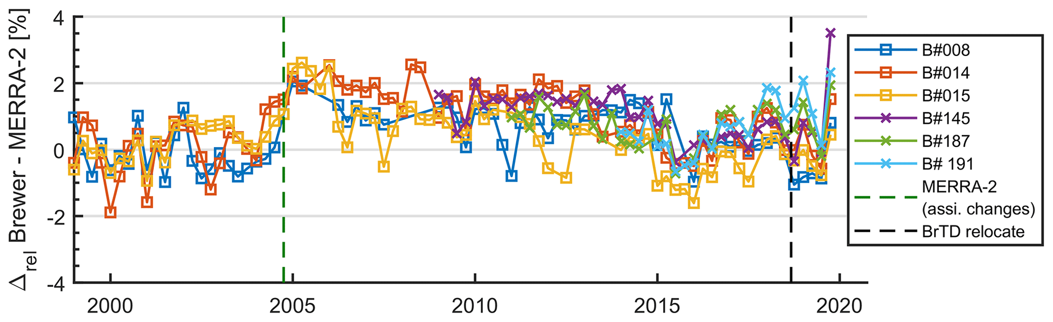
Figure 8The relative difference between the reference Brewers and MERRA-2 reanalysis. Each point represents a 3-month average. The green dash line represents the time when MERRA-2 changed its assimilation sources from SBUV-2 to MLS/OMI (causing about 2 % relative difference). The black dash line represents the time when BrT-D was relocated to Egbert.
The shift in relative difference found in 2004 was due to MERRA-2 changing its data assimilation sources (see the green dash line in Fig. 8). MERRA-2 assimilates partial column ozone data from SBUV instruments between January 1980 and September 2004. Starting from October 2004, MERRA-2 assimilates ozone profiles and columns from MLS and OMI instruments (Wargan et al., 2017). For example, the mean Brewer no. 014–MERRA-2 relative bias was 0.11 % () for the SBUV-based data assimilation, but it increased to 1.07 % after October 2004, probably due to some bias in OMI data as mentioned previously in Sect. 4.2. For the MLS/OMI-based assimilation period, the multiplicative biases between individual Brewer instruments and MERRA-2 are from 0.40 % (for Brewer no. 015) to 1.05 % (for Brewer no. 014); therefore, the relative biases between Brewers are within 0.65 %. In addition, the standard deviation of the 1-month percentage difference is on average 1.04 % for BrT and 0.87 % for BrT-D. Details of the comparison between Brewer reference instruments and the MERRA-2 reanalysis ozone dataset are summarized in Table 6.
Table 6Brewer reference instruments vs. MERRA-2 reanalysis ozone dataset.
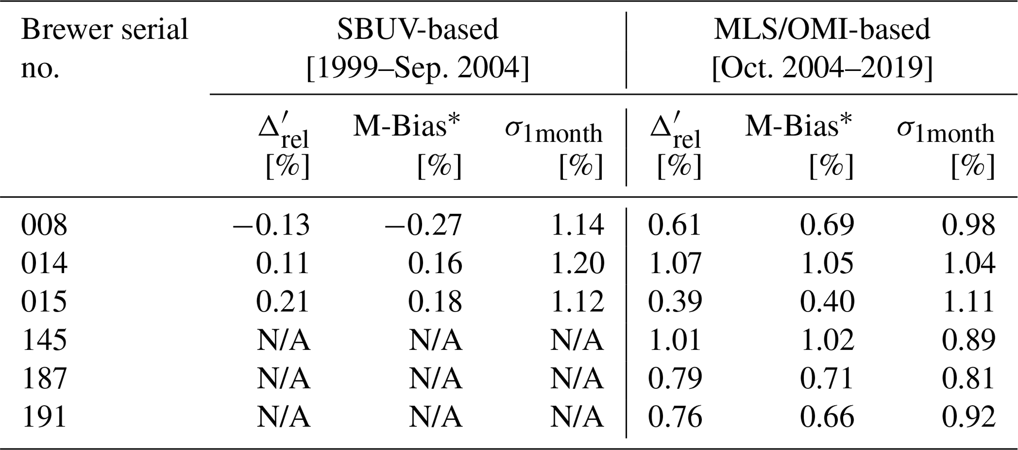
* Multiplicative bias is estimated with the slope of zero intercept linear regression. N/A: not applicable.
The performance of the European regional reference instruments (i.e., RBCC-E triad) was reported by León-Luis et al. (2018) and compared with the world reference instruments, specifically the BrT. León-Luis et al. (2018) reported that RBCC-E instruments have a mean 3-month standard deviation (δ3month) of 0.27 % and concluded that the RBCC-E instruments have 36 % lower δ3month when compared to the world reference instruments (i.e., BrT, 1984–2004 period, δ3month=0.39 %). However, the comparison was not straightforward. The Model 1 analysis carried out in León-Luis et al. (2018) did not follow the Model 1 design described in Fioletov et al. (2005) and the current work. It is worth noting that the baseline ozone should be the same (except for the offset) for all three RBCC-E instruments. This would be achieved by including the indicator functions described in Sect. 3.1.1. The 3-month standard deviations of the BrT, BrT-D and RBCC-E instruments (with corresponding data periods) are summarized in Table 7; however, the results from the RBCC-E instruments should not be directly compared to the ones in Fioletov et al. (2005) or the current work. Moreover, Stübi et al. (2017b) examined three Brewer instruments located at Arosa and found a similar performance of short-term variability. They reported that the standard deviation of short-term variability of the Arosa Brewer triad since 1998 was estimated to be about 0.36 % on the scale of a decade. The medium- to long-term stability was estimated to be within ±0.5 %.
Table 7World and European regional reference instruments' 3-month standard deviations.
* Calculated with a different method.
It is, however, important to understand that there are certain limitations in the Brewer hardware, which explain why the stability below 0.5 % is so difficult to achieve and maintain. For example, it was found that Brewer no. 015 has a particularly strong temperature dependence where the optical frame was expanding significantly faster than any other Brewer instrument. As a result, the wavelength calibration tests (HG) had to be scheduled more frequently to reduce the impact. However, we should point out that if the time interval between the HG tests is large enough, some measurements can be affected. This issue was fixed in 2017 by replacing the optical frame (details of instrument repair and upgrade history are provided in the Supplement). A second example is that the original configuration of Brewer no. 145 micrometer was found to have developed wear and became unreliable, causing some wavelength drifts and, as a result, relatively high uncertainties for Brewer no. 145 as shown in Table 7 (also see larger variations of 3-month deviations from Brewer no. 145 compared to Brewers no. 187 and no. 191 in Fig. 2a). The top and bottom micrometers were fully replaced in 2019, including all the connecting wires of the wire micrometer system.
Another example of hardware-related issues with Brewer ozone measurements is the characteristics of the ND filters used to reduce the intensity of incoming radiation (Kerr, 2010). In practice, the filters are not always neutral but may have some wavelength dependence on their transmittance. The Brewer retrieval algorithm removes effects that are linear as a function of the wavelength, but this offset may not be enough in some cases, and a shift of up to a few DU in the retrieved ozone values can occur as a result of a ND filter switch (e.g., from ND filter no. 1 in the early morning to ND filter no. 4 in the noon; Savastiouk, 2006, Sect. 4.3). Instruments with ND filters from the same manufactured batch will demonstrate almost identical spectral behaviour. Thus, these instruments may have very similar characteristics and, therefore, demonstrate high precision; however, they all may be affected by the same or similar hardware-related systematic errors. There are other hardware-related factors that affect the accuracy and precision of Brewer measurements. For example, a simple replacement of the mercury bulb that is used to ensure the instrument stability could affect total ozone measurements, creating jumps in the data record. The bulb change has the potential to affect the CalStep (calibration step, the optimal micrometer position found in the sun scan test; Savastiouk, 2006, Sect. 4.4) of the instrument. If the combined focus of the monochromator mirrors of the instrument (see Savastiouk, 2006, Sect. 4.1 for more details of instrument's optical elements) is not optimized and the illuminated filament of the mercury bulb is located in a significantly different location than the illuminated filament from the original bulb, as much as a 5 micrometer step (one micrometer step is 0.7 pm) change may be seen. For reference, the effective ozone absorption changes by approximately 1 % every three steps, so a five-step shift, which is extreme, can give an error of almost 2 % in TCO. It is best to change the mercury bulb before it completely fails so that sequential mercury tests can be performed using both bulbs to detect and address any shifts in the CalStep. It is still recommended to perform the sun scan test and verify any potential changes.
The way that the data are processed also affects the results. Siani et al. (2018) concluded that the ozone data processed by different software agree at the 1 % level; however, some differences can be found depending on the software in use. They also recommended “a rigorous manual data inspection” of the processed data and to be careful with how standard lamp (SL) test results are used. Visual data screening was also used by Stübi et al. (2017b) to eliminate outliers. However, this approach raises the question of reproducibility of the obtained results and must be carefully documented. For BrT and BrT-D's data reprocessing, we recommend using the statistical models developed in relevant studies to help the identifications of potential hardware or software issues. To keep the integrity of the world reference instruments, data reprocessing could be done only if solid evidence of imperfection of hardware or software has been found and confirmed by Brewer technicians and researchers.
Validation of satellite data is an important application of Brewer measurements and the modern satellite instruments demonstrated agreement with Brewers within 1 % (e.g., Garane et al., 2019). At the 1 % level, there are many factors that affect the comparison results. Some of the factors related to ozone absorption cross sections and their temperature dependence are well established (e.g., Redondas et al., 2014). However, the high spatial resolution of modern satellite instruments such as TROPOMI brings new challenges. Figure 9 shows that TROPOMI OVP data from the Downsview site in Toronto (centre of ground pixels within 10 km from Downsview) have a better agreement with those of the BrT-D when it was relocated to Egbert than with those of the Brewer instruments at Toronto. The difference is about 2 %, which is too large to be explained by, for example, stray light. It is likely related to a difference in viewing geometry. For the Brewer instrument, the light passes through the ozone layer once along the line between the instrument and the sun; for a satellite measurement, the light passes through the ozone layer in the same way as for ground-based measurements but then is backscattered by the atmosphere and surface toward the satellite sensor and passes through the ozone layer again. In the case of a large latitudinal gradient, the thickness of the ozone layer could be very different (Fig. 9b). As shown by the green and purple lines, the Downsview Brewers were sampling stratospheric ozone over Hamilton, while the Egbert Brewers were sampling stratospheric ozone over west of Brampton (the Brewer instruments' sampling areas were estimated with viewing geometry of Brewers and MERRA-2 ozone profiles, ground projections of the intersections between the Brewer instrument's line of sight and the modelled stratospheric ozone layer; Brampton is about 30 km west of Downsview, and Hamilton is about 70 km south-west of Downsview). The previous generations of satellite instruments had spatial resolution on the order of 50 × 50 km2 (except for OMI), and the difference in the viewing geometry had only a minor impact. However, for current and future high-resolution satellites, such as TROPOMI and TEMPO (Zoogman et al., 2014), these sampling effects should be taken into account for future satellite ozone validation works (e.g., Verhoelst et al., 2015). In general, we conclude that all these reference instruments show good long-term stability as well as meet the WMO/GAW requirements.
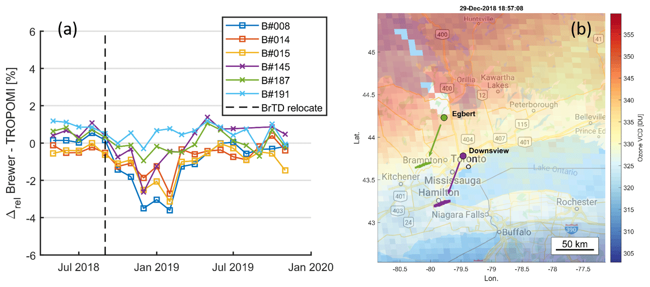
Figure 9Example of small-scale column ozone field variation. (a) Monthly relative differences between Brewers and TROPOMI total column ozone overpass measurements (for Downsview in Toronto) and (b) TROPOMI total column ozone measured on 29 December 2018 over southern Ontario, masked with Brewers' viewing directions and sampling areas. The base map is from © Google Maps.
This work assessed the long-term performance of the world Brewer reference instruments, maintained by ECCC in Toronto, Canada, in measuring total column ozone. The last assessment of the BrT was done in 2005 with two decades of ozone data records from 1984 to 2004. This work provides a more recent assessment for the BrT (1999–2019) and reports the first assessment of the BrT-D (2013–2019). It was found that both single and double reference triads met the WMO/GAW ozone monitoring requirements. Using statistical models, both BrT and BrT-D have a better than 0.5 % precision. The 3-month standard deviation of ozone values from the two triads are well within 0.5 %, with BrT-D having slightly better performance (BrT and BrT-D have mean standard deviations of 0.40 % and 0.34 %, respectively). In addition, the BrT-D has proven to have better performance in low-sun conditions (see Appendix A), which provides benefits in ozone monitoring work in the polar regions. Comparison with Pandora total ozone measurements (adjusted for temperature dependence) re-confirmed the high quality of the world Brewer reference instruments. It was found that both BrT and BrT-D have a difference of less than 0.5 %.
Further detailed error analysis shows the impacts of ETC, and ozone absorption coefficients errors for both reference triads are within ±2 % when the statistical Model 2 is used. This result is comparable to the BrT findings for data records from 1984 to 2004. When using the Pandora instrument as a reference (Model 3), the ETC and ozone absorption errors from BrT-D are slightly better than the ones from BrT (±1.5 % and ±2.0 % for BrT-D and BrT, respectively). It demonstrates that all reference instruments were well calibrated and maintained in good condition.
Differences between the measurements from the individual Brewer triad instruments and 11 satellite datasets are within −1 to +2 %. For most satellite datasets, the multiplicative bias between Brewers and satellites is well within ±1 %. The viewing geometry (or line of sight) of ground-based and satellite instruments should be considered in future high-resolution satellite ozone validation activities. Moreover, 20-year long-term reanalysis data were compared with the reference Brewers' data record. It shows that the reanalysis data have good quality, with the relative difference between the reference Brewer and the reanalysis datasets being within ±2 %. However, the changing of assimilation sources will affect the quality of the reanalysis and should be addressed in any ozone trend analysis.
The precision of the Brewer triad instruments is under 0.5 %, while the differences with the best satellite instruments and reanalysis data are close to or slightly lower than 1 %. Further improvement of Brewer total ozone observation precision may be limited by the present Brewer five-wavelength algorithm and Brewer hardware itself.
Figure A1 shows the distribution of the measurement standard deviation (δM), which is used to determine the acceptability of each DS ozone data point in the Brewer data processing algorithm. For Brewers, each final DS ozone data point is a mean of five individual measurements (performed within 3 min), and the δM is the standard deviation of these five measurements. Typically, the total column ozone values are assumed to be stable within the time of these five measurements. Thus, any DS ozone data with δM>3 DU will be removed. Figure 3a in Fioletov et al. (2005) shows the distribution of δM for BrT with μ≤3.25. Since the δM is proportional to the measured quality F divided by μ, the variability of F (among five measured F) is also influenced by μ. For example, in the range, δM of BrT has a peak value of about 1.8 DU. However, in a higher range of , δM of BrT has a peak value of about 1 DU.
Typically, Brewer DS ozone data are reported only when μ≤3.5 (note that except for this section, all Brewer DS ozone data used in this study have μ≤3.5). This is because, for single-spectrometer Brewers, measurements at high μ values are strongly affected by the stray light (Bais et al., 1996; Fioletov et al., 2000; Wardle et al., 1996). The double Brewers were designed to have low stray light (i.e., internal stray-light fraction of 10−7 and 10−5 for double and single Brewers, respectively) and showed good performance when μ>3.5 (e.g., Zhao et al., 2016). To demonstrate the benefits of low stray light in double-Brewer instruments and make a direct comparison between BrT and BrT-D, the μ range is extended to higher values (μ≤4.75) in this analysis. Figure A1 shows that for typical μ≤3.25 conditions, BrT-D has similar performance to BrT, whereas, for low solar zenith angle (SZA) conditions (e.g., ), double Brewers still have similar distributions at moderate SZA conditions. Please note that since BrT only reports ozone data with μ≤3.5, to make sure the comparison and assessment provided in this work is comparable to Fioletov et al. (2005), both BrT and BrT-D data used in any other sections are filtered with the μ≤3.5 criteria. However, the capability of measuring ozone value in low-sun conditions is very important for the ozone monitoring in polar regions where the SZA is large in early springtime. This stray-light effect is further illustrated in Fig. A2, in which the percentage difference between Pandora and BrT (BrT-D) is binned by ozone air mass factors. Figure A2 indicates that in low air mass conditions (AMF <3.5), BrT and BrT-D have similar air mass dependence, which is consistent with the results reported by Tzortziou et al. (2012) and Zhao et al. (2016). Note that Fig. A2 is similar to Fig. 15 in Zhao et al. (2016) but with an extended dataset (2013–2015 in Zhao et al., 2016, 2013–2019 in this work). It is found that the air mass dependencies of BrT and BrT-D are consistent within these two periods. Further information on the relative difference between BrT and BrT-D, in terms of air mass factor and slant column ozone, is provided in Fig. S1.
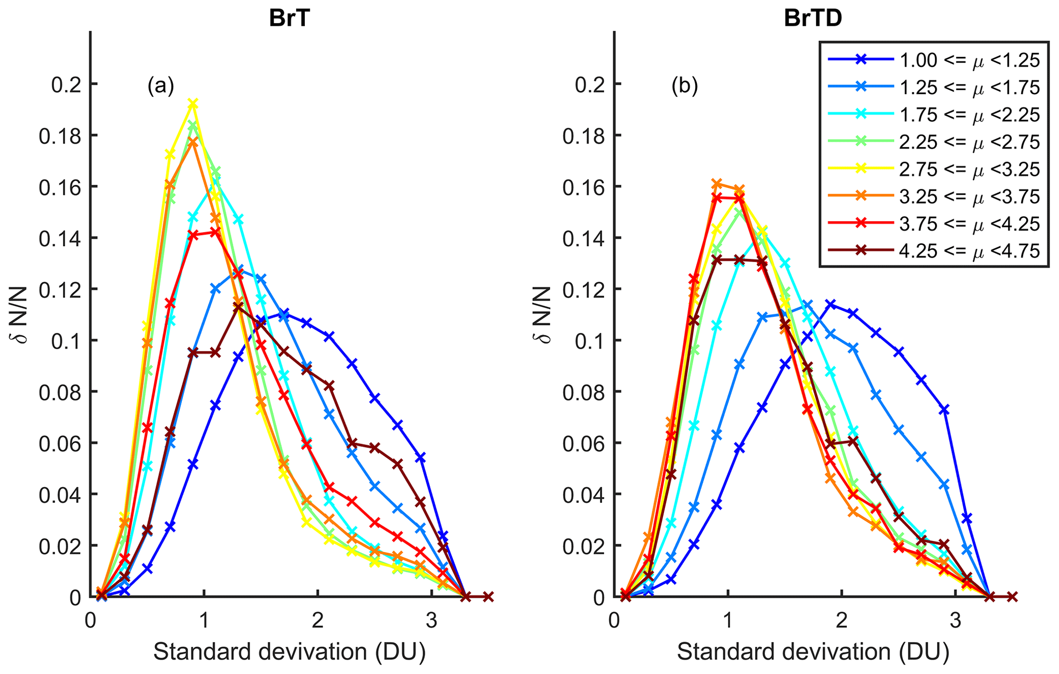
Figure A1The distribution of the standard deviations of individual DS measurements as a function of air mass value. Panel (a) shows the Brewer reference triad (BrT) data (1999–2019), and panel (b) shows the double-Brewer reference triad (BrT-D) data (2013–2019). Data from all three Brewers for each triad were used for this plot.
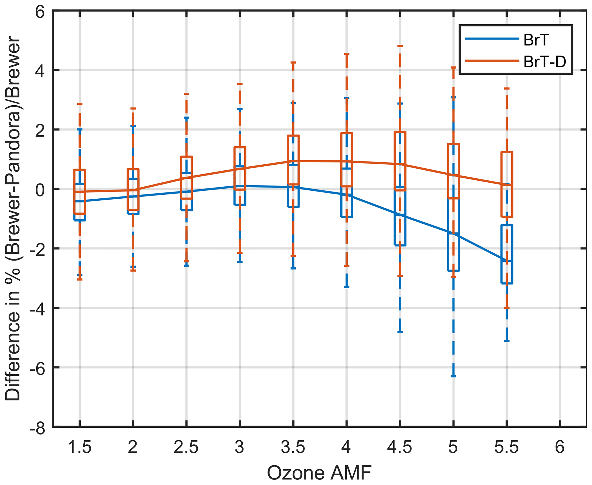
Figure A2The percentage difference between Pandora and Brewers (grouped as BrT and BrT-D) as a function of ozone air mass factor. On each box, the central mark is the median, the edges of the box are the 25th and 75th percentiles, and the whiskers extend to the most extreme data points not consider outliers.
The early operational processing run of the Brewer triad data, when reviewed through Model 3, indicated that there were some errors in the ETC and absorption values but were compensating for each other when ozone values were calculated. As a result, the used configuration produced a reasonable daily average ozone but not individual values. For example, Fig. B1 shows that the ETC error in early 2014 was as large as 4 % and the ozone absorption error was about 3 % in the operational processing version. After this observation, the data were scrutinized to find that a calibration step had inadvertently been changed by five steps from what was intended. An artificial offset in ozone absorption was introduced in an equal offset to the change in the calibration step to correct for this error. The solid line in Fig. B1 indicates the improvement made.
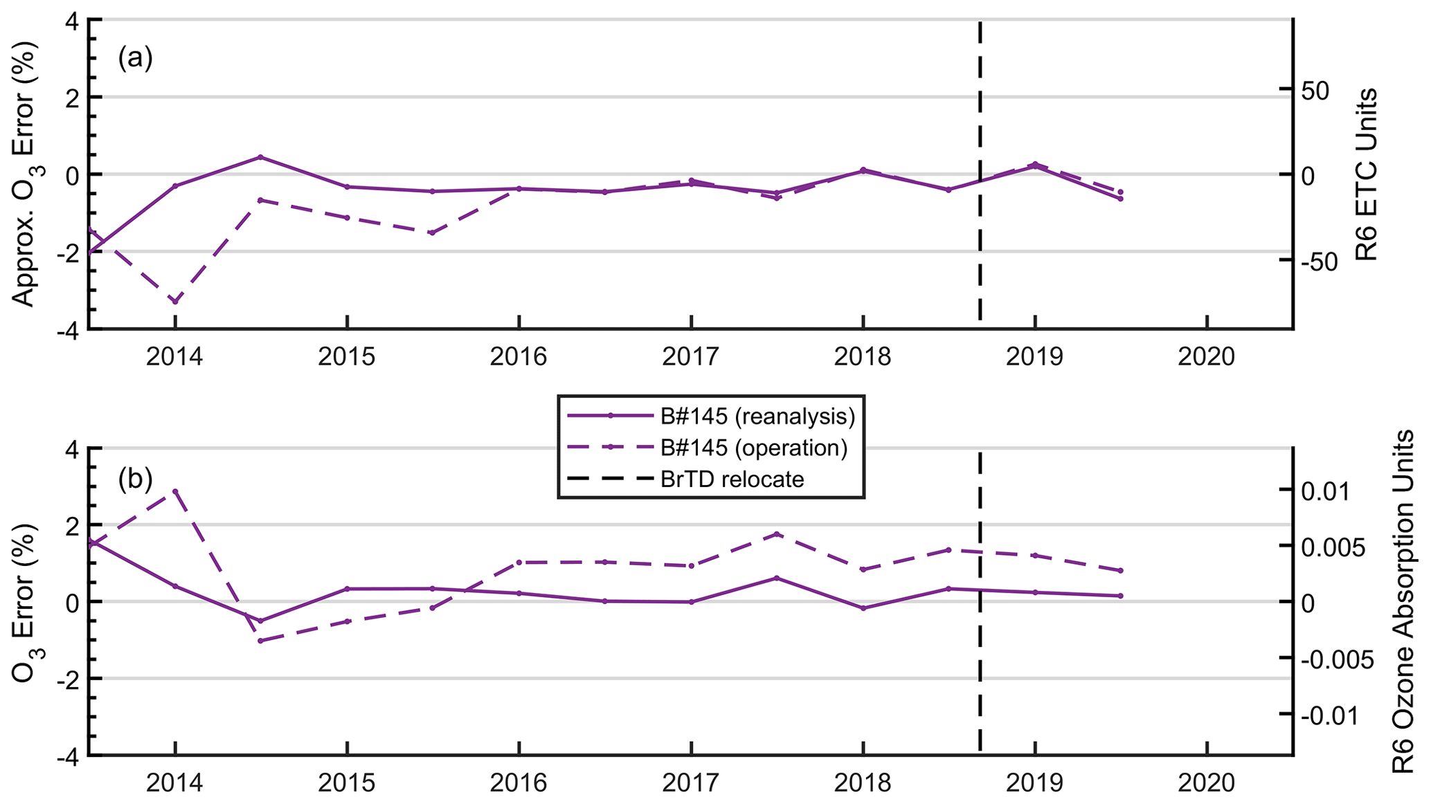
Figure B1Comparison between reprocessed and operational data from Brewer no. 145. (a) Relative systematic uncertainties in ETCs and (b) ozone absorption coefficients estimated using Model 3. Discerption of y axes in Fig. 3. Each point on the graph represents a 6-month average. The black dash line represents the time when BrT-D was relocated to Egbert.
Brewer data are available from WOUDC (https://woudc.org/, last access: 10 March 2021) (DOI: https://doi.org/10.14287/10000003, Government of Canada, 2021). Pandora data are available from the Pandonia Global Network (http://data.pandonia-global-network.org/Downsview/Pandora103s1/L2/Pandora103s1_Downsview_L2Tot_rout0p1-7.txt, Pandonia Global Network, 2021). SBUV data are available from https://acd-ext.gsfc.nasa.gov/anonftp/toms/sbuv/AGGREGATED/sbuv_aggregated_toronto_065.txt (Goddard Space Flight Center, 2021a). OMI data are available from https://avdc.gsfc.nasa.gov/pub/data/satellite/Aura/OMI/V03/L2OVP/OMDOAO3/aura_omi_l2ovp_omdoao3_v03_toronto_065.txt (Goddard Space Flight Center, 2021b) and https://avdc.gsfc.nasa.gov/pub/data/satellite/Aura/OMI/V03/L2OVP/OMTO3/aura_omi_l2ovp_omto3_v8.5_toronto_065.txt (Goddard Space Flight Center, 2021c). OMPS-NM data are available from https://doi.org/10.5067/0WF4HAAZ0VHK (Jaross, 2017). TROPOMI data are available from http://www.tropomi.eu/data-products/total-ozone-column (Netherlands Space Office, 2019). MERRA-2 data are available from https://doi.org/10.5067/VJAFPLI1CSIV (Global Modeling and Assimilation Office, 2015). Any additional data may be obtained from Xiaoyi Zhao (xiaoyi.zhao@canada.ca).
The supplement related to this article is available online at: https://doi.org/10.5194/amt-14-2261-2021-supplement.
XZ analyzed the data and prepared the manuscript, with significant conceptual input from VF and critical feedback from all co-authors. MB, RS, AO, VF, and SCL operated and managed the Canadian Brewer Spectrophotometer Network. IA, MB, AO, VF, and XZ performed all Brewer triads' data preparation. VS and MB performed independent calibrations for the Canadian Brewers. JD, XZ, VF, and SCL operated and managed the Canadian Pandora measurement program. AC, MT, and MM from the Pandonia Global Network team provided critical technical support to the Canadian Pandora measurement program. MM and MT performed the Pandora ozone harmonization work for the Downsview site in Toronto. DG and CML provided TROPOMI ozone data and supported satellite comparison.
The authors declare that they have no conflict of interest.
We gratefully acknowledge the National Oceanic and Atmospheric Administration (NOAA) and Mauna Loa Observatory staff for their support in Brewer calibrations. We thank the State Meteorological Agency of Spain (AEMET) group for hosting Brewer no. 008 and no. 145 in the 2008 calibration campaign in Izaña. We thank James Kerr for his valuable comments and suggestion for this work; James Kerr co-invented the Brewer spectrophotometer when he was a research scientist at ECCC and was previously a scientist emeritus at ECCC. We thank Nader Abuhassan, Daniel Santana Diaz, Manuel Gebetsberger, and others from SciGlob and the Pandonia Global Network (PGN) for their technical support of Canadian Pandora measurements. The PGN is a bilateral project supported with funding from the National Aeronautics and Space Administration (NASA) and the European Space Agency (ESA). We acknowledge the NASA Earth Science Division for providing OMITO3 data. The Sentinel-5 Precursor TROPOMI Level 2 product is developed with funding from the Netherlands Space Office (NSO) and processed with funding from ESA. We thank NOAA for providing NOAA SBUV data. We acknowledge the Goddard Earth Sciences Data and Information Services Center (GES DISC) for providing OMPS data. We thank the Global Modeling and Assimilation Office (GMAO) for providing MERRA-2 data.
This paper was edited by Mark Weber and reviewed by two anonymous referees.
Antón, M., López, M., Vilaplana, J. M., Kroon, M., McPeters, R., Bañón, M., and Serrano, A.: Validation of OMI-TOMS and OMI-DOAS total ozone column using five Brewer spectroradiometers at the Iberian peninsula, J. Geophys. Res., 114, D14307, https://doi.org/10.1029/2009jd012003, 2009.
Bais, A. F., Zerefos, C. S., and McElroy, C.: Solar UVB measurements with the double- and single-monochromator Brewer ozone spectrophotometers, Geophys. Res. Lett., 23, 833–836, 1996.
Bass, A. M. and Paur, R. J.: The ultraviolet cross-sections of ozone: I. The measurements, in: Atmospheric Ozone, Springer, Germany, 606–610, 1985.
Bhartia, P. K. and Wellemeyer, C. W.: OMI TOMS-V8 Total O3 algorithm, algorithm theoretical baseline document: OMI ozone products, NASA Goddard Space Flight Center, Greenbelt, Md., 2002.
Brewer, A. W.: A replacement for the Dobson spectrophotometer?, Pure Appl. Geophys., 106, 919–927, 1973.
Cede, A.: Manual for Blick Software Suite 1.6, available at: https://www.pandonia-global-network.org/wp-content/uploads/2019/11/BlickSoftwareSuite_Manual_v1-7.pdf (last access: 10 March 2021), 2019.
Cede, A., Herman, J., Richter, A., Krotkov, N., and Burrows, J.: Measurements of nitrogen dioxide total column amounts using a Brewer double spectrophotometer in direct Sun mode, J. Geophys. Res., 111, D05304, https://doi.org/10.1029/2005JD006585, 2006.
Cede, A., Tiefengraber, M., Gebetsberger, M., and Kreuter, M.: TN on PGN products “correct use” guidelines, Pandonia Global Network, available at: https://www.pandonia-global-network.org/wp-content/uploads/2020/01/LuftBlick_FRM4AQ_PGNUserGuidelines_RP_2019009_v1.pdf (last access: 13 November 2020), 2019.
Dee, D. P., Uppala, S. M., Simmons, A. J., Berrisford, P., Poli, P., Kobayashi, S., Andrae, U., Balmaseda, M. A., Balsamo, G., Bauer, P., Bechtold, P., Beljaars, A. C. M., van de Berg, L., Bidlot, J., Bormann, N., Delsol, C., Dragani, R., Fuentes, M., Geer, A. J., Haimberger, L., Healy, S. B., Hersbach, H., Hólm, E. V., Isaksen, L., Kållberg, P., Köhler, M., Matricardi, M., McNally, A. P., Monge-Sanz, B. M., Morcrette, J. J., Park, B. K., Peubey, C., de Rosnay, P., Tavolato, C., Thépaut, J. N., and Vitart, F.: The ERA-Interim reanalysis: configuration and performance of the data assimilation system, Q. J. Roy. Meteor. Soc., 137, 553–597, https://doi.org/10.1002/qj.828, 2011.
Dobson, G. M. B.: Forty Years' Research on Atmospheric Ozone at Oxford: a History, Appl. Optics., 7, 387–405, https://doi.org/10.1364/ao.7.000387, 1968.
Farman, J. C., Gardiner, B. G., and Shanklin, J. D.: Large losses of total ozone in Antarctica reveal seasonal ClOx/NOx interaction, Nature, 315, 207–210, https://doi.org/10.1038/315207a0, 1985.
Fioletov, V. E. and Ogyu, A.: Brewer Processing Software, available at: ftp://exp-studies.tor.ec.gc.ca/pub/Brewer_Processing_Software/brewer_processing_software.pdf (last access: 1 June 2020), 2008.
Fioletov, V. E., Griffioen, E., Kerr, J. B., Wardle, D. I., and Uchino, O.: Influence of volcanic sulfur dioxide on spectral UV irradiance as measured by Brewer Spectrophotometers, Geophys. Res. Lett., 25, 1665–1668, https://doi.org/10.1029/98GL51305, 1998.
Fioletov, V. E., Kerr, J. B., Hare, E. W., Labow, G. J., and McPeters, R. D.: An assessment of the world ground-based total ozone network performance from the comparison with satellite data, J. Geophys. Res., 104, 1737–1747, https://doi.org/10.1029/1998JD100046, 1999.
Fioletov, V. E., Kerr, J. B., Wardle, D. I., and Wu, E.: Correction of stray light for the Brewer single monochromator, in: Proceedings of the Quadrennial Ozone Symposium, Hokkaido University, Sapporo, Japan, 3–8 July 2000, p. 37, 2000.
Fioletov, V. E., Kerr, J. B., Wardle, D. I., Krotkov, N. A., and Herman, J. R.: Comparison of Brewer ultraviolet irradiance measurements with total ozone mapping spectrometer satellite retrievals, Opt. Eng., 41, 3051–3062, https://doi.org/10.1117/1.1516818, 2002.
Fioletov, V. E., Kerr, J. B., McElroy, C. T., Wardle, D. I., Savastiouk, V., and Grajnar, T. S.: The Brewer reference triad, Geophys. Res. Lett., 32, L20805, https://doi.org/10.1029/2005GL024244., 2005.
Fioletov, V. E., McLinden, C. A., McElroy, C. T., and Savastiouk, V.: New method for deriving total ozone from Brewer zenith sky observations, J. Geophys. Res., 116, D08301, https://doi.org/10.1029/2010JD015399, 2011.
Flynn, L., Long, C., Wu, X., Evans, R., Beck, C. T., Petropavlovskikh, I., McConville, G., Yu, W., Zhang, Z., Niu, J., Beach, E., Hao, Y., Pan, C., Sen, B., Novicki, M., Zhou, S., and Seftor, C.: Performance of the Ozone Mapping and Profiler Suite (OMPS) products, J. Geophys. Res., 119, 6181–6195, https://doi.org/10.1002/2013JD020467, 2014.
Garane, K., Koukouli, M.-E., Verhoelst, T., Lerot, C., Heue, K.-P., Fioletov, V., Balis, D., Bais, A., Bazureau, A., Dehn, A., Goutail, F., Granville, J., Griffin, D., Hubert, D., Keppens, A., Lambert, J.-C., Loyola, D., McLinden, C., Pazmino, A., Pommereau, J.-P., Redondas, A., Romahn, F., Valks, P., Van Roozendael, M., Xu, J., Zehner, C., Zerefos, C., and Zimmer, W.: TROPOMI/S5P total ozone column data: global ground-based validation and consistency with other satellite missions, Atmos. Meas. Tech., 12, 5263–5287, https://doi.org/10.5194/amt-12-5263-2019, 2019.
Global Modeling and Assimilation Office (GMAO): MERRA-2 tavg1_2d_slv_Nx: 2d,1-Hourly,Time-Averaged,Single-Level,Assimilation,Single-Level Diagnostics V5.12.4, Greenbelt, MD, USA, Goddard Earth Sciences Data and Information Services Center (GES DISC), https://doi.org/10.5067/VJAFPLI1CSIV, 2015.
Goddard Space Flight Center, Nasa: SBUV data, available at: https://acd-ext.gsfc.nasa.gov/anonftp/toms/sbuv/AGGREGATED/sbuv_aggregated_toronto_065.txt, last access: 10 March 2021a.
Goddard Space Flight Center, Nasa: OMI data, available at: https://avdc.gsfc.nasa.gov/pub/data/satellite/Aura/OMI/V03/L2OVP/OMDOAO3/aura_omi_l2ovp_omdoao3_v03_toronto_065.txt, last access: 10 March 2021b.
Goddard Space Flight Center, Nasa: OMI data, available at: https://avdc.gsfc.nasa.gov/pub/data/satellite/Aura/OMI/V03/L2OVP/OMTO3/aura_omi_l2ovp_omto3_v8.5_toronto_065.txt, last access: 10 March 2021c.
Government of Canada: Total Ozone – hourly observations, Data set, https://doi.org/10.14287/10000003, 2021.
Gueymard, C. A.: The sun's total and spectral irradiance for solar energy applications and solar radiation models, Sol. Energy, 76, 423–453, https://doi.org/10.1016/j.solener.2003.08.039, 2004.
Herman, J., Cede, A., Spinei, E., Mount, G., Tzortziou, M. and Abuhassan, N.: NO2 column amounts from ground-based Pandora and MFDOAS spectrometers using the direct-sun DOAS technique: Intercomparisons and application to OMI validation, J. Geophys. Res., 114, D13307, https://doi.org/10.1029/2009JD011848, 2009.
Herman, J., Evans, R., Cede, A., Abuhassan, N., Petropavlovskikh, I., and McConville, G.: Comparison of ozone retrievals from the Pandora spectrometer system and Dobson spectrophotometer in Boulder, Colorado, Atmos. Meas. Tech., 8, 3407–3418, https://doi.org/10.5194/amt-8-3407-2015, 2015.
Jaross, G.: OMPS-NPP L2 NM Ozone (O3) Total Column swath orbital V2, Greenbelt, MD, USA, Goddard Earth Sciences Data and Information Services Center (GES DISC), https://doi.org/10.5067/0WF4HAAZ0VHK, 2017.
Karppinen, T., Redondas, A., García, R. D., Lakkala, K., McElroy, C. T., and Kyrö, E.: Compensating for the Effects of Stray Light in Single-Monochromator Brewer Spectrophotometer Ozone Retrieval, Atmos.-Ocean, 53, 66–73, https://doi.org/10.1080/07055900.2013.871499, 2015.
Kazadzis, S., Bais, A., Kouremeti, N., Gerasopoulos, E., Garane, K., Blumthaler, M., Schallhart, B., and Cede, A.: Direct spectral measurements with a Brewer spectroradiometer: absolute calibration and aerosol optical depth retrieval, Appl. Opt., 44, 1681–1690, https://doi.org/10.1364/AO.44.001681, 2005.
Kerr, J. B.: New methodology for deriving total ozone and other atmospheric variables from Brewer spectrophotometer direct sun spectra, J. Geophys. Res., 107, 4731, https://doi.org/10.1029/2001JD001227, 2002.
Kerr, J. B.: The Brewer Spectrophotometer, in UV Radiation in Global Climate Change: Measurements, Modeling and Effects on Ecosystems, edited by: Gao, W., Slusser, J. R., and Schmoldt, D. L., Springer, Berlin, Heidelberg, 160–191, 2010.
Kerr, J. B., McElroy, C. T., and Olafson, R. A.: Measurements of ozone with the Brewer ozone spectrophotometer, in: Proceedings of the Quadrennial Ozone Symposium, Boulder, USA, 4–9 August 1980, 74–79, 1981.
Kerr, J. B., Evans, W. F. J., and Asbridge, I. A.: Recalibration of Dobson Field Spectrophotometers with a Travelling Brewer Spectrophotometer Standard, in Atmospheric Ozone, edited by: Zerefos, C. S. and Ghazi, A., Springer, Netherlands, Dordrecht, 381–386, 1985.
Kerr, J. B., Asbridge, I. A., and Evans, W. F. J.: Intercomparison of total ozone measured by the Brewer and Dobson spectrophotometers at Toronto, J. Geophys. Res., 93, 11129–11140, https://doi.org/10.1029/JD093iD09p11129, 1988.
Kerr, J. B., McElroy, C. T., and Wardle, D. I.: The Brewer instrument calibration center 1984–1996, in: Proceedings of the Quadrennial Ozone Symposium, L'Aquila, Italy, 12–21 September 1996, pp. 915–918, 1998.
Kramarova, N. A., Nash, E. R., Newman, P. A., Bhartia, P. K., McPeters, R. D., Rault, D. F., Seftor, C. J., Xu, P. Q., and Labow, G. J.: Measuring the Antarctic ozone hole with the new Ozone Mapping and Profiler Suite (OMPS), Atmos. Chem. Phys., 14, 2353–2361, https://doi.org/10.5194/acp-14-2353-2014, 2014.
Kroon, M., Veefkind, J. P., Sneep, M., McPeters, R. D., Bhartia, P. K., and Levelt, P. F.: Comparing OMI-TOMS and OMI-DOAS total ozone column data, J. Geophys. Res., 113, D16S28, https://doi.org/10.1029/2007jd008798, 2008.
Kurucz, R. L.: New atlases for solar flux, irradiance, central intensity, and limb intensity, Memorie della Società Astronomica Italiana Supplement, 8, 189–191, 2005.
Kyrö, E.: Intercomparison of total ozone data from Nimbus 7 TOMS, the Brewer UV Spectrophotometer and SAOZ UV-Visible Spectrophotometer at High Latitudes Observatory, Sodankylä, Geophys. Res. Lett., 20, 571–574, https://doi.org/10.1029/93GL00806, 1993.
Labow, G. J., McPeters, R. D., Bhartia, P. K., and Kramarova, N.: A comparison of 40 years of SBUV measurements of column ozone with data from the Dobson/Brewer network, J. Geophys. Res., 118, 7370–7378, https://doi.org/10.1002/jgrd.50503, 2013.
León-Luis, S. F., Redondas, A., Carreño, V., López-Solano, J., Berjón, A., Hernández-Cruz, B., and Santana-Díaz, D.: Internal consistency of the Regional Brewer Calibration Centre for Europe triad during the period 2005–2016, Atmos. Meas. Tech., 11, 4059–4072, https://doi.org/10.5194/amt-11-4059-2018, 2018.
Marenco, F., di Sarra, A., and Luisi, J. D.: Methodology for determining aerosol optical depth from brewer 300–320-nm ozone measurements, Appl. Opt., 41, 1805–1814, https://doi.org/10.1364/AO.41.001805, 2002.
McPeters, R. D., Bhartia, P. K., Krueger, A. J., Herman, J. R., Wellemeyer, C. G., Seftor, C. J., Jaross, G., Torres, O., Moy, L., Labow, G., Byerly, W., Taylor, S. L., Swissler, T., and Cebula, R. P.: Earth Probe Total Ozone Mapping Spectrometer (TOMS) Data Products User's Guide, available at: https://ozoneaq.gsfc.nasa.gov/media/docs/epusrguide.pdf (last access: 10 March 2021), 1998.
Netherlands Space Office: Total Ozone Column, available at: http://www.tropomi.eu/data-products/total-ozone-column (last access: 10 March 2021), 2019.
Pandonia Global Network: Pandora 103 total column ozone data at Downsview, Toronto, Canada, available at: http://data.pandonia-global-network.org/Downsview/Pandora103s1/L2/Pandora103s1_Downsview_L2Tot_rout0p1-7.txt, last access: 10 March 2021.
Ramaswamy, V., Schwarzkopf, M. D., and Shine, K. P.: Radiative forcing of climate from halocarbon-induced global stratospheric ozone loss, Nature, 355, 810–812, 1992.
Redondas, A., Evans, R., Stuebi, R., Köhler, U., and Weber, M.: Evaluation of the use of five laboratory-determined ozone absorption cross sections in Brewer and Dobson retrieval algorithms, Atmos. Chem. Phys., 14, 1635–1648, https://doi.org/10.5194/acp-14-1635-2014, 2014.
Redondas, A., Carreño, V., León-Luis, S. F., Hernández-Cruz, B., López-Solano, J., Rodriguez-Franco, J. J., Vilaplana, J. M., Gröbner, J., Rimmer, J., Bais, A. F., Savastiouk, V., Moreta, J. R., Boulkelia, L., Jepsen, N., Wilson, K. M., Shirotov, V., and Karppinen, T.: EUBREWNET RBCC-E Huelva 2015 Ozone Brewer Intercomparison, Atmos. Chem. Phys., 18, 9441–9455, https://doi.org/10.5194/acp-18-9441-2018, 2018.
Rienecker, M. M., Suarez, M. J., Gelaro, R., Todling, R., Bacmeister, J., Liu, E., Bosilovich, M. G., Schubert, S. D., Takacs, L., and Kim, G.-K.: MERRA: NASA's modern-era retrospective analysis for research and applications, J. Climate, 24, 3624–3648, 2011.
Rimmer, J. S., Redondas, A., and Karppinen, T.: EuBrewNet – A European Brewer network (COST Action ES1207), an overview, Atmos. Chem. Phys., 18, 10347–10353, https://doi.org/10.5194/acp-18-10347-2018, 2018.
Savastiouk, V.: Improvements to the direct-sun ozone observations taken with the Brewer spectrophotometer, PhD Thesis, York University, Canada, 2006.
Serdyuchenko, A., Gorshelev, V., Weber, M., Chehade, W., and Burrows, J. P.: High spectral resolution ozone absorption cross-sections – Part 2: Temperature dependence, Atmos. Meas. Tech., 7, 625–636, https://doi.org/10.5194/amt-7-625-2014, 2014.
Siani, A. M., Frasca, F., Scarlatti, F., Religi, A., Diémoz, H., Casale, G. R., Pedone, M., and Savastiouk, V.: Examination on total ozone column retrievals by Brewer spectrophotometry using different processing software, Atmos. Meas. Tech., 11, 5105–5123, https://doi.org/10.5194/amt-11-5105-2018, 2018.
Solomon, S., Garcia, R. R., Rowland, F. S., and Wuebbles, D. J.: On the depletion of Antarctic ozone, Nature, 321, 755–758, https://doi.org/10.1038/321755a0, 1986.
Staehelin, J., Renaud, A., Bader, J., McPeters, R., Viatte, P., Hoegger, B., Bugnion, V., Giroud, M., and Schill, H.: Total ozone series at Arosa (Switzerland): Homogenization and data comparison, J. Geophys. Res., 103, 5827–5841, https://doi.org/10.1029/97JD02402, 1998.
Stolarski, R. S., Krueger, A. J., Schoeberl, M. R., McPeters, R. D., Newman, P. A., and Alpert, J. C.: Nimbus 7 satellite measurements of the springtime Antarctic ozone decrease, Nature, 322, 808–811, https://doi.org/10.1038/322808a0, 1986.
Stolarski, R. S., Bloomfield, P., McPeters, R. D., and Herman, J. R.: Total Ozone trends deduced from Nimbus 7 Toms data, Geophys. Res. Lett., 18, 1015–1018, https://doi.org/10.1029/91gl01302, 1991.
Stübi, R., Schill, H., Klausen, J., Vuilleumier, L., Gröbner, J., Egli, L., and Ruffieux, D.: On the compatibility of Brewer total column ozone measurements in two adjacent valleys (Arosa and Davos) in the Swiss Alps, Atmos. Meas. Tech., 10, 4479–4490, https://doi.org/10.5194/amt-10-4479-2017, 2017a.
Stübi, R., Schill, H., Klausen, J., Vuilleumier, L., and Ruffieux, D.: Reproducibility of total ozone column monitoring by the Arosa Brewer spectrophotometer triad, J. Geophys. Res., 122, 4735–4745, https://doi.org/10.1002/2016JD025735, 2017b.
Thuillier, G., Floyd, L., Woods, T. N., Cebula, R., Hilsenrath, E., Hersé, M., and Labs, D.: Solar irradiance reference spectra for two solar active levels, Adv. Space Res., 34, 256–261, https://doi.org/10.1016/j.asr.2002.12.004, 2004.
Tzortziou, M., Herman, J. R., Cede, A., and Abuhassan, N.: High precision, absolute total column ozone measurements from the Pandora spectrometer system: Comparisons with data from a Brewer double monochromator and Aura OMI, J. Geophys. Res., 117, D16303, https://doi.org/10.1029/2012JD017814, 2012.
Van Hoosier, M. E.: Solar ultraviolet spectral irradiance data with increased wavelength and irradiance accuracy, in: Proceedings of Ultraviolet Atmospheric and Space Remote Sensing: Methods and Instrumentation, International Society for Optics and Photonics, Denver, CO, United States, 4-9 August 1996, 57–64, 1996.
Vaziri Zanjani, Z., Moeini, O., McElroy, T., Barton, D., and Savastiouk, V.: A calibration procedure which accounts for non-linearity in single-monochromator Brewer ozone spectrophotometer measurements, Atmos. Meas. Tech., 12, 271–279, https://doi.org/10.5194/amt-12-271-2019, 2019.
Veefkind, J. P. , de Haan, J. F., Brinksma, E. J., Kroon, M., and Levelt, P. F.: Total ozone from the ozone monitoring instrument (OMI) using the DOAS technique, IEEE T. Geosci. Remote, 44, 1239–1244, https://doi.org/10.1109/tgrs.2006.871204, 2006.
Verhoelst, T., Granville, J., Hendrick, F., Köhler, U., Lerot, C., Pommereau, J.-P., Redondas, A., Van Roozendael, M., and Lambert, J.-C.: Metrology of ground-based satellite validation: co-location mismatch and smoothing issues of total ozone comparisons, Atmos. Meas. Tech., 8, 5039–5062, https://doi.org/10.5194/amt-8-5039-2015, 2015.
Wardle, D. I., McElroy, C. T., Kerr, J. B., Wu, E., and Lamb, K.: Laboratory tests on the double Brewer spectrophotometer, in: Proceedings of the Quadrennial Ozone Symposium, L'Aquila, Italy, 12–21 September 1996, 997–1000, 1996.
Wargan, K., Labow, G., Frith, S., Pawson, S., Livesey, N., and Partyka, G.: Evaluation of the Ozone Fields in NASA's MERRA-2 Reanalysis, J. Climate, 30, 2961–2988, https://doi.org/10.1175/JCLI-D-16-0699.1, 2017.
WMO: World Meteorological Organization Global Atmosphere Watch – Global Atmosphere Watch Measurements Guide, WMO TD No. 1073, available at: https://library.wmo.int/doc_num.php?explnum_id=4632 (last access: 24 November 2020), 2001.
WMO: Scientific assessment of ozone depletion: 2018, Global Ozone Research and Monitoring Project, World Meteorological Organization, Geneva, Switzerland, 2018.
Zerefos, C. S., Eleftheratos, K., Kapsomenakis, J., Solomos, S., Inness, A., Balis, D., Redondas, A., Eskes, H., Allaart, M., Amiridis, V., Dahlback, A., De Bock, V., Diémoz, H., Engelmann, R., Eriksen, P., Fioletov, V., Gröbner, J., Heikkilä, A., Petropavlovskikh, I., Jarosławski, J., Josefsson, W., Karppinen, T., Köhler, U., Meleti, C., Repapis, C., Rimmer, J., Savinykh, V., Shirotov, V., Siani, A. M., Smedley, A. R. D., Stanek, M., and Stübi, R.: Detecting volcanic sulfur dioxide plumes in the Northern Hemisphere using the Brewer spectrophotometers, other networks, and satellite observations, Atmos. Chem. Phys., 17, 551–574, https://doi.org/10.5194/acp-17-551-2017, 2017.
Zhao, X., Fioletov, V., Cede, A., Davies, J., and Strong, K.: Accuracy, precision, and temperature dependence of Pandora total ozone measurements estimated from a comparison with the Brewer triad in Toronto, Atmos. Meas. Tech., 9, 5747–5761, https://doi.org/10.5194/amt-9-5747-2016, 2016.
Zhao, X., Weaver, D., Bognar, K., Manney, G., Millán, L., Yang, X., Eloranta, E., Schneider, M., and Strong, K.: Cyclone-induced surface ozone and HDO depletion in the Arctic, Atmos. Chem. Phys., 17, 14955–14974, https://doi.org/10.5194/acp-17-14955-2017, 2017.
Zhao, X., Bognar, K., Fioletov, V., Pazmino, A., Goutail, F., Millán, L., Manney, G., Adams, C., and Strong, K.: Assessing the impact of clouds on ground-based UV–visible total column ozone measurements in the high Arctic, Atmos. Meas. Tech., 12, 2463–2483, https://doi.org/10.5194/amt-12-2463-2019, 2019.
Zoogman, P., Jacob, D. J., Chance, K., Liu, X., Lin, M., Fiore, A., and Travis, K.: Monitoring high-ozone events in the US Intermountain West using TEMPO geostationary satellite observations, Atmos. Chem. Phys., 14, 6261–6271, https://doi.org/10.5194/acp-14-6261-2014, 2014.
- Abstract
- Introduction
- Datasets
- Comparison methods
- Assessment results
- Discussion
- Conclusion
- Appendix A: Distribution of standard deviations of individual DS measurements
- Appendix B: Model 3 analysis improvement examples
- Data availability
- Author contributions
- Competing interests
- Acknowledgements
- Review statement
- References
- Supplement