the Creative Commons Attribution 4.0 License.
the Creative Commons Attribution 4.0 License.
 | 06 Apr 2021
Applicability of the VisiSize D30 shadowgraph system for cloud microphysical measurements
Moein Mohammadi
Szymon P. Malinowski
A commercial shadowgraph system, the Oxford Lasers VisiSize D30, originally designed to characterize industrial and agricultural sprays, was tested with respect to its application for measuring cloud microphysical properties such as droplet size distribution and number concentration. A laboratory experiment with a dense stream of polydisperse cloud-like droplets indicated a strong dependence of the depth of field, and thus also the sample volume, on particle size. This relationship was determined and a suitable correction method was developed to improve estimations of droplet number concentration and size distribution. The spatial homogeneity of the detection probability inside the sample volume and the minimum droplet diameter providing uniform detection were examined. A second experiment with monodisperse droplets produced by a Flow Focusing Monodisperse Aerosol Generator (FMAG) verified the sizing accuracy and demonstrated reasonable agreement between the instruments. Effects of collisions and the evaporation of droplets produced by the FMAG were observed. Finally, when the instrument was applied to sample atmospheric clouds at a mountain-based observatory, it performed reliably during a 3-week-long field experiment. Based on the laboratory and field tests, recommendations concerning the use of the instrument for cloud droplet measurements were formulated.
- Article
(11838 KB) - Full-text XML
- BibTeX
- EndNote


Atmospheric clouds predominantly consist of water droplets. Cloud droplet number concentration (DNC) and size distribution (DSD) constitute the key parameters for the quantitative microphysical description of clouds, and attract enormous attention in contemporary atmospheric science, mostly due to their crucial importance to cloud lifetimes, radiative effects and rain formation (Devenish et al., 2012).
There are two general approaches to measuring cloud microphysical properties: in situ sampling at airborne platforms or ground-based stations and remote sensing, which involves applying inverse retrieval techniques to data collected by satellites, radars and radiometers. Researchers employing either of these strategies face intrinsic difficulties. For instance, in situ methods often have to account for a dependence of the sample volume on particle size or air flow velocity, nonlinearity of the Mie scattering intensity with respect to droplet size, and aerodynamic effects related to the flow around or inside the instrument or aircraft; they may involve harsh conditions (including icing, wetting and temperature changes); and they can necessitate the handling of large datasets or instantaneous data processing. Remote sensing provides information with limited spatial resolution; hence the microphysical properties they measure represent only averages or integrals over relatively large volumes, which might be too simplistic to characterize inhomogeneous or multilayered cloud fields. On top of that, the retrievals are often dependent on the assumption of a specific size distribution or specific vertical structure of the atmosphere. In general, in situ measurements are considered fundamental, as they offer instrumental access to individual droplets within a sampling volume. The results obtained in situ are then used to derive and validate inversion routines to be used in remote-sensing applications.
Among the in situ techniques, one can distinguish two branches differing in sampling style:
-
instruments that detect and count droplets one by one almost continuously as they pass through a very small active probe volume provide individual droplet properties and their interarrival times,
-
instruments that capture images or another spatial representation of droplets inside a larger sampling volume provide individual droplet properties and information on their spatial arrangement.
The first branch is represented by a number of spectrometers that use light scattering for droplet detection and sizing, e.g. a Forward Scattering Spectrometer Probe (FSSP, e.g. Cooper, 1988; Brenguier et al., 1998; Gerber et al., 1999; de Araújo Coelho et al., 2005), a Cloud Droplet Probe (CDP, e.g. McFarquhar et al., 2007; Lance et al., 2010; Lance, 2012), a Cloud and Aerosol Spectrometer (CAS, e.g. Lance, 2012; Glen and Brooks, 2013; Barone et al., 2019) and a Phase Doppler Interferometer (PDI, e.g. Bachalo and Houser, 1984; Chuang et al., 2008; Kumar et al., 2019). In practice, they sample a quasi-one-dimensional portion of air passing through the active sampling region. The exact volume sampled in unit time depends on the velocity with respect to the instrument. Therefore, meaningful estimation of the DNC requires information on air velocity. Moreover, due to the small cross section of the probe volume, there is an upper limit for the measurable droplet size. For instance, the range of diameters that are measurable by a CDP is 2–50 µm.
Volumetric methods (the second branch) usually do not rely on the scattering intensity of an individual droplet for sizing, and their sampling volumes do not depend on the velocity of the flow, but consecutive air samples collected instantaneously can be quite distant from each other, particularly when such methods are used on fast-moving airborne platforms. This class of techniques is represented e.g. by shadowgraphy and holography. Neglecting the effect of imperfect focusing, a shadow image is a two-dimensional projection of all the objects onto the camera plane. It can be rapidly processed to detect particles and obtain relevant statistics. Holograms require extensive processing to digitally reconstruct the shapes and arrangement of objects in three dimensions (Fugal et al., 2009). Both methods allow position, size and shape to be discerned, meaning that not only spherical droplets but also e.g. ice crystals can be studied.
Holographic systems have been successfully deployed on research aircraft (HOLODEC, Fugal and Shaw, 2009, and HALOHolo, Schlenczek, 2017a; Schlenczek et al., 2017b; Lloyd et al., 2020), at mountain-based observatories (HOLIMO, Henneberger et al., 2013), on mountain cable cars (HoloGondel, Beck et al., 2017) and on balloon-borne platforms (HoloBalloon, Ramelli et al., 2020). Typically, those instruments have a resolution of 6 µm, a sample volume (SV) of about 15 cm3, and take a few holograms per second, which results in a sample volume rate (SVR) of around 90 cm3 s−1. The recent HoloBalloon setup features an SV of 22.5 cm3 and a frame rate of 80 fps, which gives an SVR of 1800 cm3 s−1. Shadowgraphy has been used e.g. in a Cloud Particle Imager (CPI, Lawson et al., 2001; Connolly et al., 2007), an airborne instrument to observe ice particles and supercooled droplets in the size range of 2.3–2300 µm (Woods et al., 2018). The typical SV is much smaller than in holography (about 0.04 cm3); however, the frame rate is much higher (400 fps), which gives an SVR of about 16 cm3 s−1. Moreover, Rydblom and Thörnberg (2016) have designed a system to investigate icing conditions for wind turbines based on shadow images. Nevertheless, despite both its simplicity and many insightful laboratory experiments, e.g. concerning droplet collisions (Bordás et al., 2013; Bewley et al., 2013), shadowgraphy is not the first-choice method for cloud droplet measurements.
In order to explore in detail the advantages and disadvantages of shadowgraphy for cloud microphysical applications, we used a commercial shadowgraph system – the VisiSize D30 from Oxford Lasers Ltd. (Kashdan et al., 2003, 2004), originally designed for the diagnosis of agricultural and industrial sprays – to measure the DNC and DSD in warm clouds. In the study, two series of laboratory experiments were performed which aimed at verifying the reliability of detection and accuracy of sizing under conditions resembling atmospheric clouds. They were followed by a field experiment targeting real cloud at a mountaintop observatory.
The present paper is structured as follows. Section 2 describes the instrument and the measurement principle. Section 3 provides an analysis of detection reliability and homogeneity, which affect the DNC and DSD results. These parameters were investigated using polydisperse water droplets. Section 4 focuses on sizing accuracy, which was studied using a monodisperse droplet population. Based on the experiments, corrections to the standard algorithm implemented in the instrument's software are suggested. Finally, in Sect. 5 we present selected results obtained during the first application of the instrument to atmospheric clouds. The last section summarizes the findings and discusses our conclusions concerning the further usage of the VisiSize D30 system for cloud research.
The VisiSize D30 is a complete shadowgraph system manufactured by Oxford Lasers Ltd. (Oxon, United Kingdom) and designed to characterize particles in various suspensions. Common industrial applications include, among others, the characterization of agricultural sprays, paint sprays, consumer aerosols, fire extinguishers and automotive fuel injectors.
2.1 Hardware description
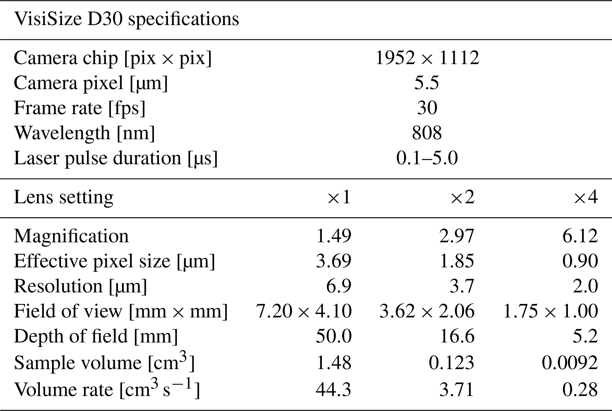
The two main parts of the setup are an infrared diode pulse laser with diffuser and a digital camera with a suitable lens objective (see Fig. 1). The lens magnification can be changed manually to adjust the resolution and the sample volume to the object studied. For three selected options, instrument calibration was performed by the supplier. The capabilities of the system at those settings are listed in Table 1.
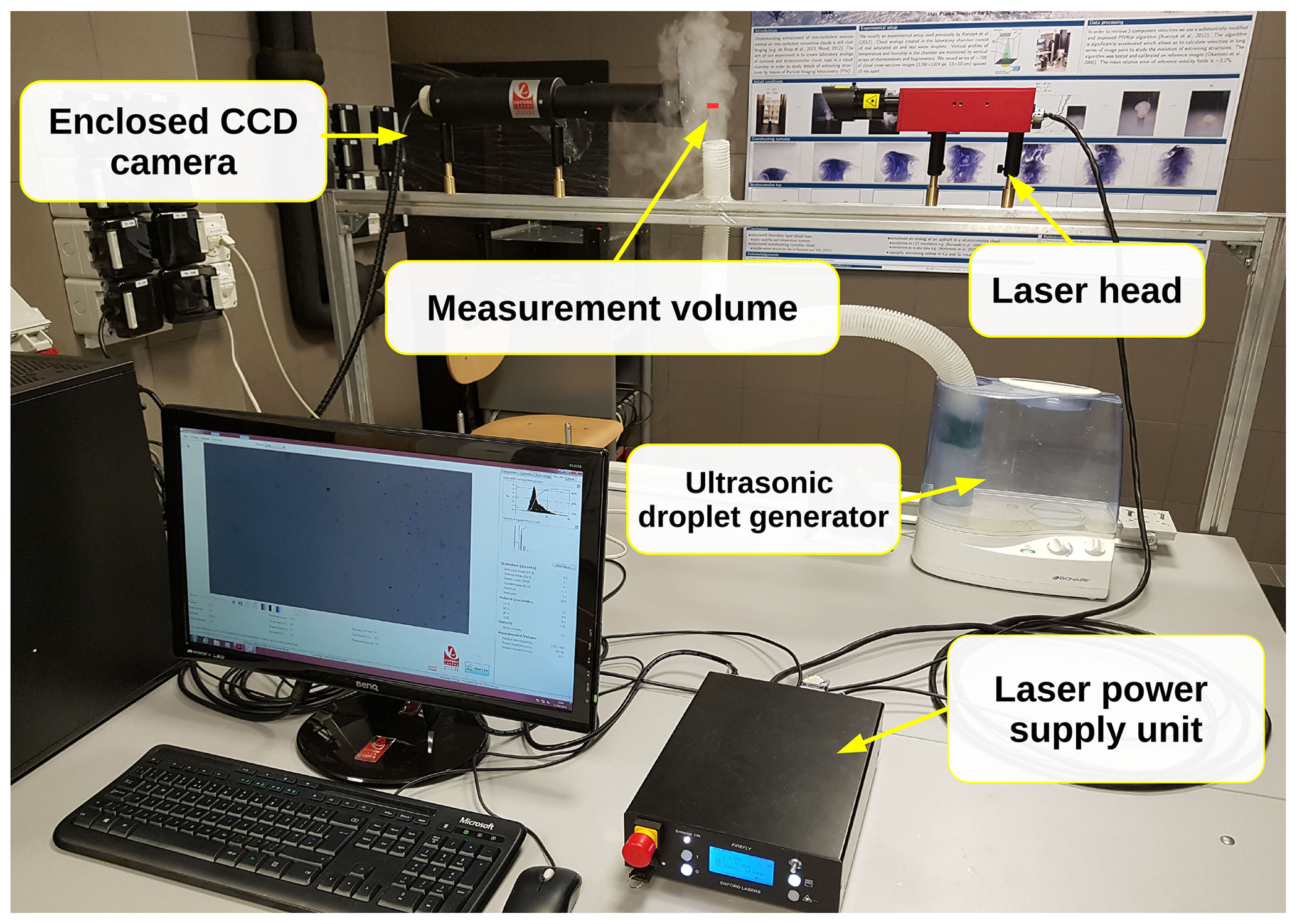
Figure 1Experimental setup for studying the detection properties (see Sect. 3 for details). The main parts of the VisiSize D30 are an infrared pulse laser with a diffuser (top right) and a CCD camera with the lens objective enclosed in a waterproof housing (top left). Water droplets produced with an ultrasonic droplet generator are measured while passing through the sample volume (top middle) located close to the camera.
Table 1Properties of the VisiSize D30 system for three different lens magnification settings provided by Oxford Lasers Ltd.
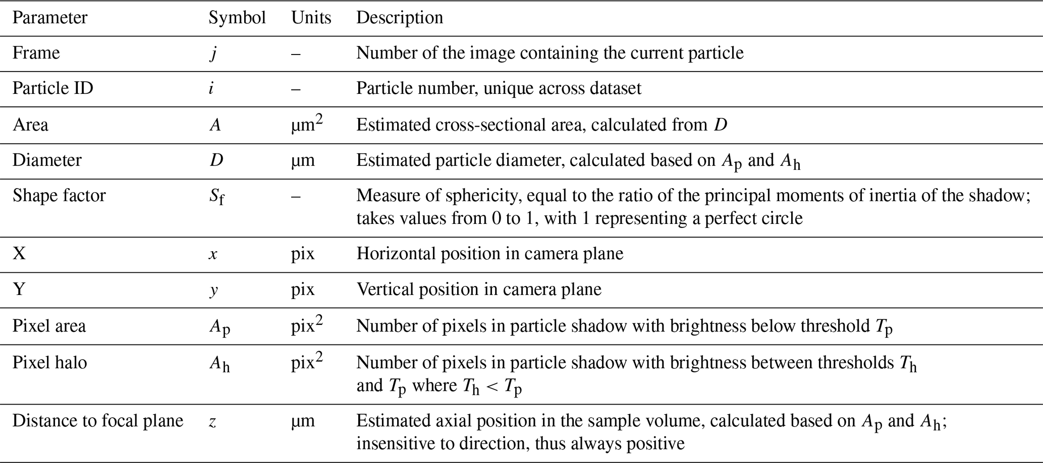
The working principle of the system is the following. The region of interest is illuminated from behind by the diffused (incoherent) expanded laser light beam, and shadow images of droplets are collected at up to 30 frames or pairs of frames per second with a digital camera. The laser and the camera are jointly triggered so that a single laser pulse “freezes” the motion of droplets present within the measurement volume during each frame capture. Droplets detected inside the depth of field (DOF) are then measured based on their shadow images, and statistics regarding the concentration or size distribution are built by processing the series of images. It should be noted that there is also an option to measure droplet velocity in the imaging plane by comparing pairs of consecutive frames and measuring droplet displacement between them. The captured images are either processed in real time to determine particle positions and sizes (live mode) or stored as graphic files (capture mode). In the former case, the output is only a list of particles together with their properties (droplet file). Specific quantities included in the droplet file are explained in Table 2. The second complementary output file contains the system settings used and a measurement summary with some basic statistics for the recorded droplet set (summary file). With the capture mode, one can analyse captured images later by tuning some parameters, or the raw genuine view of the particles can be accessed (see Fig. 3 in Sect. 3.1). However, the total uninterrupted measurement time is then limited by the available computer RAM.
Table 2Explanation of the parameters reported in the output droplet file together with the symbols used to denote them in the text.
2.2 Principle of droplet detection and sizing
The measurement principle applied in the VisiSize system was explained by Kashdan et al. (2003, 2004). It stems from the basic observation that with increasing defocus (particle displacement from the focal plane of the camera lens), the image of the object becomes increasingly blurred, which hinders the proper estimation of the size of the shadow. On the other hand, the range of axial positions guaranteeing acceptable sharpness of the shadow is usually quite limited. As a consequence, the probability of detecting a particle inside such a restricted SV is often insufficient to collect meaningful statistics for the suspension in a reasonable timeframe. To overcome the difficulties described above, Kashdan et al. (2003) applied a method that compensates for the effects of imperfect focus. Basically, the displacement from the focal plane is estimated from the degree of image blur, i.e. the gradient of brightness at the edge of the inner dark shadow. In their implementation, two threshold limits are determined for each analysed picture based on the histogram of pixel brightness. Both of them lie between the background intensity and the level corresponding to dark centres of particle shadows (see Fig. 2). The upper threshold Tp separates the background from the particle image. All pixels below this value are assumed to belong to the effective total particle image area Ap (of equivalent diameter Dp). The lower threshold Th distinguishes between the dark shadow interior and an outer grey “halo”. Pixels with intensities between Th and Tp are counted to produce the estimate for the particle halo area Ah (of equivalent width Dh). Therefore, Ah belongs to and is smaller than Ap.
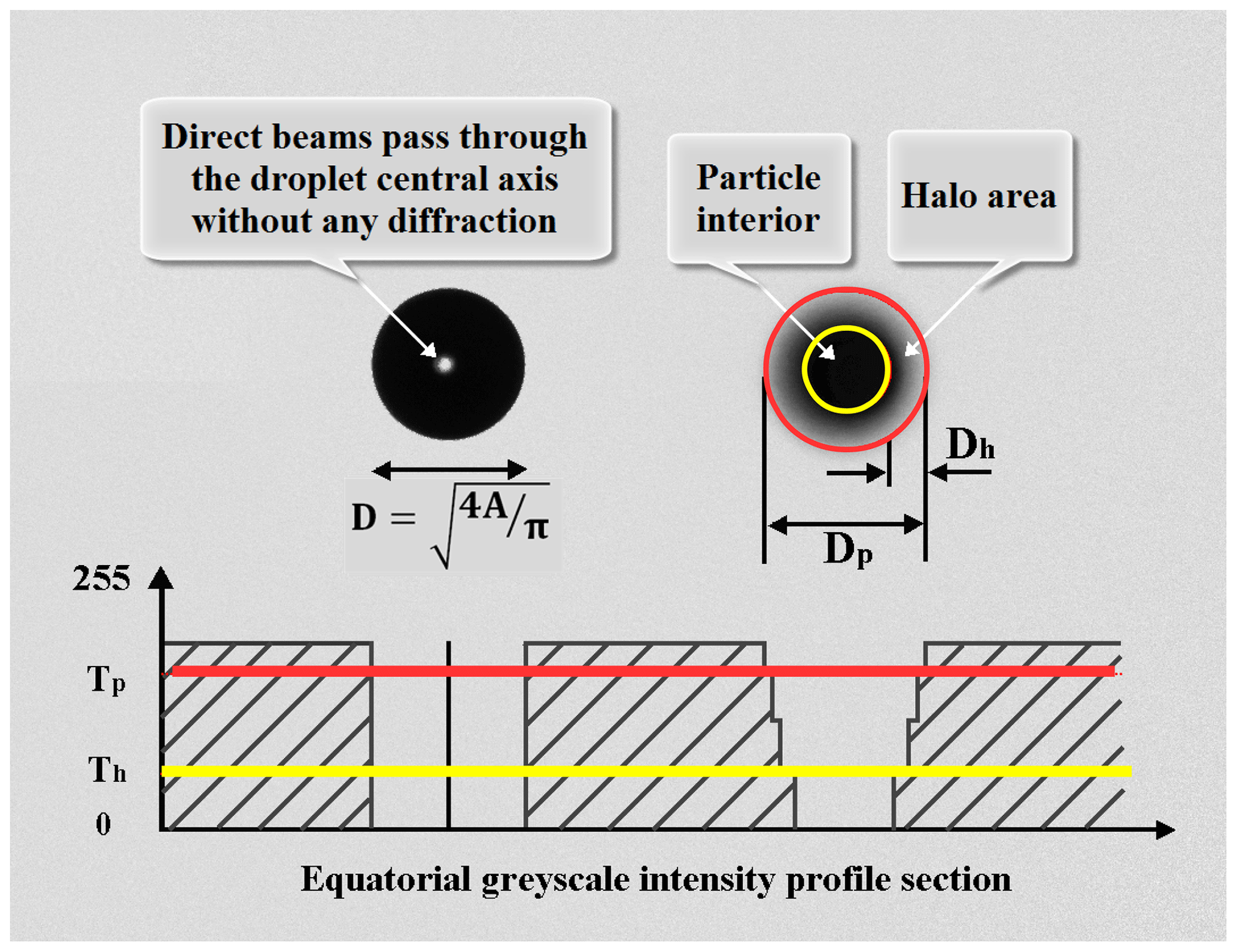
Figure 2Schematic representation of the threshold method showing shadow images of two sample droplets – an in-focus droplet (left) and a defocused droplet (right) – above greyscale intensity profiles illustrating the applied thresholds.
With increasing defocus distance, the total area of the particle image grows due to the blurring until it fades away at some point into the background, making the object no longer distinguishable. Note that the halo area Ah grows faster than the total area Ap because it extends in both the outer and inner directions, taking over the background and the interior pixels, respectively. Ideally, Ah should tend to zero for an object standing exactly in the focal plane. However, this is never the case due to intrinsic diffraction caused by the finite aperture of the lens. This effect can be particularly important for a small object of a similar size to the optical resolution of the system.
The particle total area Ap and halo area Ah can be regarded as directly measured quantities. Both the true particle diameter D and the estimated defocus distance z are derived from them. The exact conversion is determined separately for each lens setting using experimental calibration. The pictures of calibration targets of known sizes are taken at known distances from the focal plane. When applying the sizing algorithm to the collected data, functions are fitted to approximate the relationships Ap(D,z) and Ah(D,z). For the present VisiSize D30 model, calibration was performed by Oxford Lasers for three possible lens magnification settings (×1, ×2 and ×4), and these calibrations were incorporated into the software.
Ah grows with the distance between the actual particle position and the focal plane. The halo is formed exactly around the dark interior of the shadow, i.e. each point on an initially very sharp edge spreads equally in all directions, smoothing the intensity gradient and creating a halo for which the area scales with the perimeter length and the amount of defocus. For almost circular objects, the perimeter is proportional to the diameter, which leads to the scaling Ah∼Dz. However, when it is not in the focal plane, even a point source is mapped to a circle of confusion in the image plane (camera chip). Therefore, Ah should be a growing function of z, even when the size D tends to zero. The simple linear relation that satisfies the above properties is
where a1 and a2 are calibration constants for a given lens magnification.
As described above, with increasing defocus distance z, the halo around the dark interior develops at the cost of both the background pixels and the inner shadow pixels. The whole Ah is included in the total particle pixel area Ap, so only the outward growth affects the value of Ap. The outward part of the shell is larger than the inward one; hence the proportionality factor is close to but slightly higher than 0.5. Obviously, in the focal plane, the image area is dependent on the true cross section of the physical object, but Ap is composed of pixels of finite size, which disturbs the perfect representation of smooth shapes. Consequently, the effective diameter length may decrease by an amount that is of the order of the pixel size. Moreover, diffraction comes into play even for the focal plane, hindering perfect imaging – objects always appear slightly larger than they are in reality. This is particularly important for small droplets. This diameter enlargement due to diffraction should be of the order of the optical resolution of the lens system. All of these effects can be taken into account by using a formula of the form
where the constants a3, a4, a5 and pix describe the halo blurring, pixelization, diffraction and effective pixel size, respectively. Note that Ap is specified as the number of pixels; hence the unit conversion factor pix2 is needed. Having obtained the values of Ah and Ap from the image of the specific particle, both the diameter D and the defocus distance z can be calculated by inverting Eqs. (1) and (2).
3.1 Diagnostic experiment
The first diagnostic laboratory experiment was carried out to characterize instrument performance in terms of detection probability and homogeneity, which affect the statistics for the DNC and DSD. A dense stream of polydisperse water droplets was generated using an ultrasonic humidifier, as in the study by Korczyk et al. (2012), who measured the droplets and found them to be 2–20 µm in diameter in general (see their Fig. 1). Differences in delivery method and in ambient conditions could result in slightly different spectra. In our setup, the cloud of droplets was delivered from the humidifier to the SV through a 4 cm wide, 70 cm long circular plastic pipe. Care was taken to fill the whole shadowgraph SV with the stream of droplets, though neither the flow nor the particle field were exactly homogeneous. The flow velocity was estimated to be of the order of 10 cm s−1, and the direction of the flow was aligned horizontally from left to right (i.e. the exit from the pipe was perpendicular to what is shown in Fig. 1). For each of the three lens settings (×1, ×2, ×4), the laser power was adjusted to achieve the optimal background brightness for the pictures, and a 10 min long measurement in live mode was performed. Figure 3 presents an example of an image captured during the experiment. Statistics reported by the software for each run are listed in Table 3.
Table 3Statistics of the laboratory experiment with polydisperse droplets for different lens magnification settings.


Figure 3A typical shadow image of droplets produced by an ultrasonic droplet generator. The image was taken during laboratory tests with a camera lens magnification setting of ×2.
3.2 Focus rejection and depth of field
Results of the experiment show that certain conditions limit the range of permissible values of the halo area Ah (see Fig. 4); the same is true of the total particle area Ap. At a sufficiently large distance from the focal plane, the particle image starts to fade into the background, meaning that it is no longer distinguishable. Simultaneously, the halo takes over almost the whole particle image. To avoid measuring objects with signal-to-noise ratios that do not permit proper sizing, a simple rejection limit is exercised by the software:
Importantly, it is not possible for the user to deactivate this option in version 6.5.39 of the software.
This condition imposes an upper limit on the range of values that Ah can take. On the other hand, the minimum halo area can be estimated by the diffraction at the particle's edge, as diffraction effects cannot be avoided even when there is perfect in-focus placement. The lower limit for the halo can be approximated by the product of the perimeter length πD times the diffraction constant a5 (see Fig. 4). Note that large values of Ah are attained only for relatively large droplets and at far defocus. Accordingly, for a given diameter, the range of the total particle area Ap is also limited. It can grow with defocus distance z but only to the point where the halo constitutes 95 % of the image; otherwise the particle is rejected.
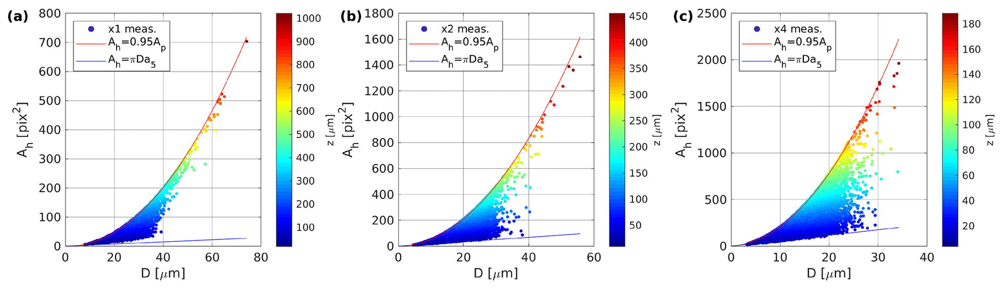
Figure 4Range of halo areas Ah observed in the measurement results as functions of the droplet diameter D and defocus distance z for different lens magnification settings: (a) ×1, (b) ×2, (c) ×4.
According to Eqs. (1) and (2), the halo grows linearly with droplet diameter whereas the total image area grows quadratically. This means that for a given defocus distance z, the halo should constitute a larger fraction of the whole image for small droplets than for large ones. With increasing z, the halo fills the image much sooner for small objects, and their shadows fade more quickly into the background, meaning that they are no longer detectable. Such qualitative reasoning explains the intuitive fact that the range of z within which the object can be detected depends on the object size. For instance, the effective SV depends on the cloud droplet diameter, which in turn affects the measurement of the DSD.
Kashdan et al. (2003) showed that, to a reasonable accuracy, the range of possible defocus distances (depth of field, DOF) grows linearly with particle diameter. The proportionality factor a6 comes from experimental calibration. The measurement volume V is then equal to the product of the default DOF and the effective area of the camera sensor S (field of view, FOV).
In a summary file generated by the software, this formula is applied to calculate the volumes Vk corresponding to the consecutive size bins , where the integers denote bin numbers.
However, the volumes calculated with this method are not correct for small particles such as typical droplets in atmospheric clouds. The reason for this is that the focus rejection condition (Ah<0.95Ap) limits the acceptable defocus distance z. Hereafter, this limit will be denoted z95, in contrast to the previously introduced zdef. The specific value can be obtained by using Eqs. (1) and (2) to expand the inequality of the focus rejection criterion in Eq. (3).
The effect of the above condition is illustrated in Fig. 5. For all the droplets measured in the diagnostic experiment, Eq. (3) leads to a much stronger limit on the effective SV than Eq. (4) does. Predicted ranges of defocus distance agree very well with the maximum values zmax found in the experimental dataset. The discrepancy observed for the largest sizes is related to the poor statistics, i.e. the small number of large droplets, which are infrequent in the measured plume. It can be shown that focus rejection defines the true SV for small particles, whereas it usually has no effect for large particles such as raindrops (z95>zdef). The exact critical size depends on the lens settings and the respective calibration. It can be calculated that the relative difference between the two values drops below 10 % for particles larger than 210, 260 and 50 µm with lens settings of ×1, ×2, ×4, respectively. Considering the population of droplets, the choice of the DOF limit would have only a minor effect on the results.
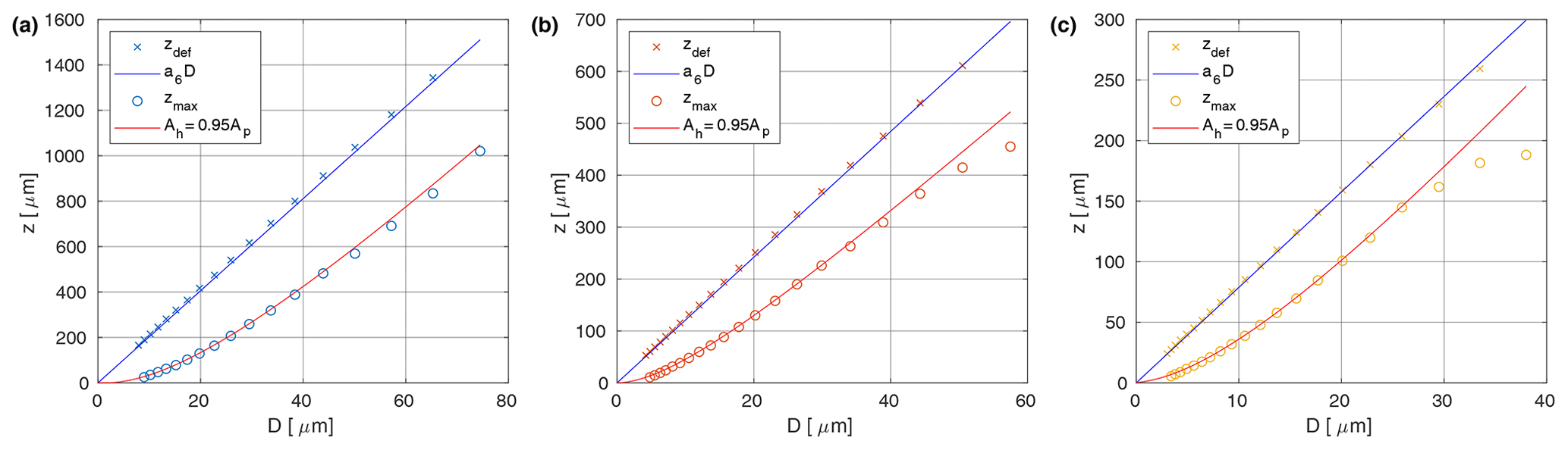
Figure 5The maximum range of the defocus distance z for each size bin as derived from the volumes listed in the summary file (crosses), the corresponding actual maximum values zmax found in the experimental data (circles), and two analytical approximations: the default zdef and the corrected z95. Measurement series are shown for three lens magnification settings: (a) ×1, (b) ×2, (c) ×4.
3.3 Effective sample volumes
The size-dependent DOF has to be accounted for when calculating the DSD based on shadowgraph images. Moreover, the image processing procedure includes a border rejection mechanism which excludes all the objects touching the outer edge of the picture because the sizing of those objects would be strongly biased. Thus, the effective cross-sectional area of the camera sensor, the FOV, is reduced by the margin equal to the diameter under consideration. Cloud droplets are orders of magnitude smaller than the whole FOV, so such a correction – although reasonable – would not exert much influence on the final results and may often be neglected. However, it is significant for large drops, i.e. rain. The default SVs in calculations of DSD are given by
where Lx and Ly denote the size of the FOV in µm and k is the number of a size bin.
However, as explained above, the default solution does not account for the DOF limitation due to the focus rejection condition. Hence, the corrected SVs can be defined as follows:
If the total number of bins K is small or the spread of droplet diameters present in a dataset is particularly large, then the range of sizes for objects belonging to one bin might be significant. For that reason, it would be sensible to introduce an SV prescribed for the particular droplet of interest. Calculating the DSD using individual volumes should be more precise from a physical point of view. On the other hand, such an approach requires access to the list of all droplets, whereas corrected and default methods need only the accumulated number of particles within the bins.
Based on the above discussion, the effect of the choice of the DOF limit on the effective SV around a droplet is shown schematically in Fig. 6.
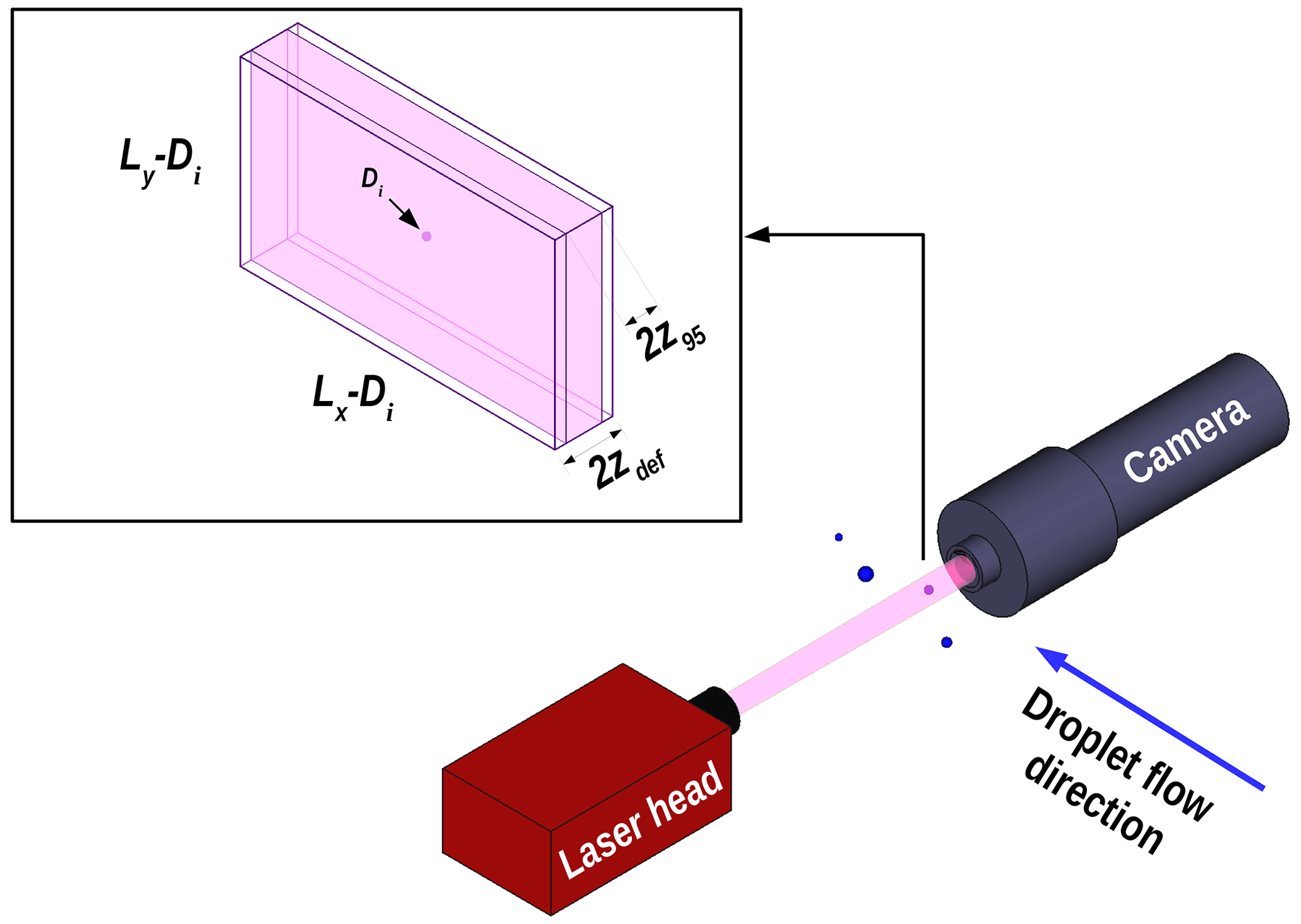
Figure 6Schematic illustrating the difference between the default and the corrected/individual sample volumes with the same field of view but different depths of field (zdef vs. z95).
3.4 Correction of the concentration and size distribution
Proper quantitative measures of the particle concentration and size distribution in a given suspension should allow for meaningful comparisons between measurement series, instruments and experimental conditions. As explained, the effective SV depends on the object size. Additionally, from a practical perspective, size bins with widths that grow with increasing diameter are usually employed. In order to characterize the spatial arrangement and size distribution of droplets, we introduce a parameter corresponding to the number of counts normalized to both spatial position and size. This quantity has units of and should be interpreted as the local probability density function (PDF) of droplet diameter at point normalized to sum to the local total droplet concentration (number per unit volume, DNC) at this point. Then
corresponds to the global PDF of droplet diameters, and
corresponds to the global DNC.
Ideally, should describe physical reality. It cannot be easily estimated from the measurement just by binning the results because the instrument is only able to detect a particle of a size D inside the limited range of z due to the size dependent DOF. If one divides the ranges of the four variables into bins to construct 4-dimensional grid cells, counts the entries in each cell, and normalizes them to the 4D volumes of the cells, some of the grid cells in the experimentally obtained would be missing information. For the same reason, the limits of the integral in Eq. (9) along dz should depend on D.
Where the DSD is concerned, NVD(D) has an advantage over the simple PDF since values from the former can be compared between measurement series. For the same phenomenon, a different lens setting should yield the same results. In order to estimate NVD(D), the number of particles within a given size range needs to be divided by the respective size-dependent volume. Specifically, for the three methods depicted in the previous subsection,
where is the number of counts within bin k, is the bin width, and F is simply the number of frames included in the analysed series.
DSDs obtained with Eqs. (11)–(13) for the laboratory experiment indicate (see Fig. 7) that NVD(D) values are significantly underestimated by the default method. This is not surprising, since Eq. (4) generates SVs which are much larger than the true ones. On the other hand, there is no significant difference between the corrected and individual SVs). This observation suggests that even when data on individual droplets cannot be accessed (such data are usually present in a particle file), a reasonable DSD can be obtained by correcting the accumulated counts listed in a summary file.
Figure 7 compares the size distributions of droplets generated using the same device but measured with different lens settings. If each configuration resolves the full range of diameters present in the spray, the lines should follow each other. Instead, the results only agree (approximately) for larger droplets, which can be explained by the increase in instrument resolution with the magnification used. The plots suggest that the true minimum droplet size for uniform detection is ∼6 µm for ×2 and ∼12 µm for ×1. As expected, these values are greater than 3.7 and 6.9 µm, respectively, which are the resolutions in the vicinity of the focal plane according to the manufacturer. Unfortunately, the results do not allow such a limit to be determined for a lens magnification setting of ×4. It can be speculated that it is roughly 4 µm i.e. above the focal plane resolution (about 2 µm) and below the uniform detection limit for magnification ×2 (6 µm).
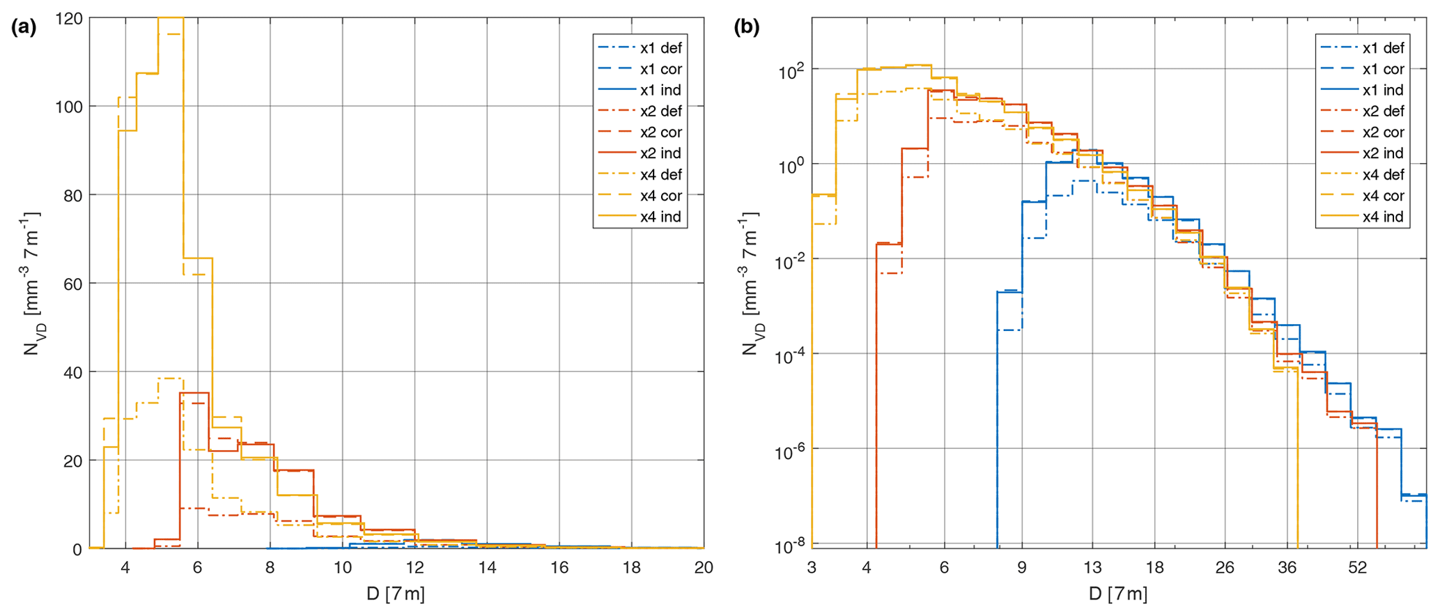
Figure 7Comparison of the droplet size distributions obtained with three methods – default (def), corrected (cor) and individual (ind) – for the three measurement series obtained with different lens magnification settings. The same data are plotted on (a) linear and (b) logarithmic scales.
The total DNC NV can be calculated by suitable integration with respect to the whole range of diameters, which is in practice the sum over the bins for the default and corrected methods or the sum over individual counts for the individual method:
With information about the DNC and DSD to hand, simple statistics that characterize clouds, such as the mean droplet diameter or higher order moments of the distribution (mean surface diameter D2, mean volume diameter D3 and effective diameter De), can be calculated. The liquid water content (LWC) can be estimated by summing the volumes of the droplets measured. Because the DSD varies with the method and lens setting used, the resulting mean diameters and LWC will also vary. Table 4 summarizes the results obtained for the polydisperse stream produced by an ultrasonic generator. DNC is about 3–4 times larger for the corrected and individual methods than for the default one. In all cases, statistics for the diameter are lower for the new methods than for the default. This can be explained by noting that the largest relative difference in SVs between the methods appears for the smallest droplets (see Fig. 5), so it is their contribution to the DSD that changes most.
Table 4Results of a laboratory experiment with polydisperse droplets: comparison of different methods that are used to estimate size-dependent sample volumes.

3.5 Homogeneity of detection
One of the important properties characterizing a particle sizing instrument, apart from the extent of the SV, is the homogeneity of detection inside that volume. Perfect homogeneity can be defined as the case in which the probability of detecting the given particle of interest is the same everywhere as long as the particle appears to be at a position within the respective SV, regardless of how complicated the boundaries of the SV are. If the probability depends on the position of the particle in space, the results obtained with the system may be biased. This is particularly important when calculating the droplet spatial arrangement measures, e.g. the nearest neighbour distance or the radial distribution function (Larsen and Shaw, 2018).
In the present study, the quality of detection was evaluated for the VisiSize D30 shadowgraph system based on a long record for a plume of water droplets produced by an ultrasonic droplet generator. As stated earlier (Sect. 3.1), the stream of droplets was assumed to extend further than the SV in each direction. Unfortunately, independent information on whether the DNC inside the visible plume was uniform was not available. One would expect it to drop from its maximal value at the centre towards the edges, where intensive mixing takes place between cloudy and clear air portions. Nevertheless, the mixing zone was observed to be outside the SV – at least on average, because in general the outflow was quite dynamic. Therefore, statistics integrated over time will be analysed in this section. To allow us to draw conclusions regarding the detection, it was assumed that the real physical conditions were homogeneous on average, i.e. during the experiment, the flow filled each part of the entire SV with an identical concentration of droplets with identical properties (e.g. DSD).
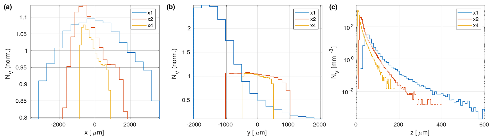
Figure 8Dependence of the droplet concentration on the (a) horizontal, (b) vertical and (c) axial positions.
The experimental results integrated over size, time and distance to the focal plane mostly point to a relatively constant average droplet concentration with respect to the two principal directions of the camera sensor – horizontal and vertical. The calculated average concentration drops significantly close to the edges of the FOV (not shown), which is expected considering the border rejection procedure. Figure 8a and b show the normalized droplet concentrations and integrated over size and other dimensions and divided by the total concentration. These are shown in order to highlight the relative dependence on position inside the sample volume. Generally, the values decrease gradually from the maximum (located left of centre) to the sides in the horizontal direction and from the bottom to the top in the vertical direction. Aside from very close to the edges, the relative differences are of the order of 10 %. These are small enough to be potentially caused by plume nonuniformity. The y dependence of the concentration is more pronounced for larger droplets (above 12 µm, not shown here), which may be due to gravity sorting. However, for the series recorded with a lens setting of ×1, the concentration falls with height y by a factor of more than 10 from the bottom to the top of the FOV. We speculate that this effect originates from the instrument, as the difference is too large (almost exponential) and the timescale is too short for the effect to be due solely to gravity sorting of the droplets in the plume. The probable reason is nonuniform illumination of the scene. Although nonuniformities can be compensated for by performing background normalization (such a function is included in the software), the signal-to-noise ratio of an individual particle shadow can still depend on the position, with consequences for the detection probability. Due to an extensive halo, some particles might have been rejected. This problem with illumination could stem from imperfect manual alignment of the laser with the camera, but it should be noted that achieving satisfactory light conditions with a lens setting of ×1 or lower is challenging. There are no such issues at higher settings, as the FOV is then smaller and fits easily inside the uniform core of the laser beam.
The axial dependence is more difficult to evaluate because the acceptable DOF depends on both the particle size and the lens setting. As expected, the average concentration decreases with z, since only droplets which are large enough can be counted at longer distances (see Fig. 8c). This trend is a result of the coexisting effects of DOF limitation and the shape of the real DSD, as large droplets constitute only a minor fraction of all the droplets. Interestingly, there are far fewer droplets at low z than in the maximum located further from the focal plane, regardless of the lens setting. Such unphysical behaviour might stem from the sizing algorithm, which calculates the z position from the halo area according to the inverted Eq. (1). Small particles such as those observed in the experiment are blurred not only due to defocus but also in the focal plane itself, which causes them to be assigned to distances that are larger than their true distances. Equation (1) assumes that there is no halo for the focal plane z=0, which is not realistic due to diffraction. Thus, every particle has a nonzero halo Ah, resulting in z>0 for all the shadows.
Moreover, it should be noted that at larger z, the concentration rises with pixel size (and falls with magnification, depending on the lens setting chosen; see Table 1). This behaviour is related to the DOF limits (Eq. 4) and respective curves plotted in Fig. 5. Comparison between the three magnifications implies that for any fixed distance z larger than roughly 117 µm, the lower limit of the detectable size range increases with the magnification, i.e. a wider spectrum of droplets can be counted at lens setting ×1 than at ×2 and ×4. For example, at z=150 µm, the lens settings ×1, ×2 and ×4 allow for the detection of droplets larger than 21.4, 22.2 and 26.4 µm in diameter, respectively.
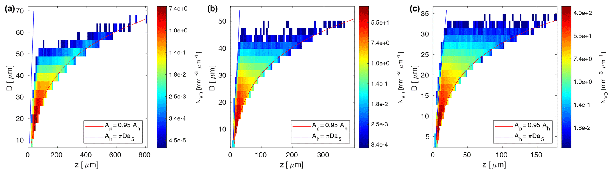
Figure 9Variability of droplet detection properties in the size–space domain for lens settings of (a) ×1, (b) ×2 and (c) ×4.
However, the probability of detection might depend on both the position in space and the particle size. Therefore, the cross-correlated dependence was examined and is illustrated in the form of 2-dimensional (z,D) maps in Fig. 9. It is easy to recognize the limitation introduced by the focus rejection criterion, which also controls the effective SV (red line). On the other hand, the minimum distance zmin for a given diameter is well approximated by assuming that the halo area in the focal plane is equal to the diffraction term (Ah=πDa5), analogously to Fig. 4, and solving Eq. (1) for z (blue line).
What is more, the DSD seems to change with the distance z from the focal plane. A growing fraction of small particles is not detected as the distance z increases, which is a simple consequence of the focus rejection criterion. However, NVD(z,D) for D well above the focus rejection limit (red line) is expected not to change with the distance z. At lens setting ×1, large droplets are only present far from the focal plane, and the concentration of droplets of a given size grows with z. Such behaviour suggests that the sizing procedure for the measurements at lens setting ×1 may not have worked properly. Possibly, insufficient brightness of the pictures caused the halo area to be overestimated at the cost of the inner particle shadow. According to the sizing Eqs. (1) and (2), this leads to overestimation of the defocus distance and underestimation of the diameter.
As a consequence, the authors discourage the use of lens setting ×1 in studies of cloud droplets. The large minimum particle size for uniform detection reported earlier (∼12 µm) makes this an option of limited utility anyway. Instead, ×1 may be useful for measurements of drizzle drops. In order to avoid the illumination and signal-to-noise issue described above, we would suggest that, as a rule of thumb, the lower limit should be an order of magnitude larger than the effective pixel size (3.69 µm). On the other hand, the objects need to fit into the FOV, so the largest measured size should be a few times smaller than the shortest dimension (4.1 mm), which eventually results in a conservative range of roughly 40–400 µm. However, thus far, insufficient data on drizzle have been collected to be able to confirm this expectation experimentally.
In experimental runs with higher magnifications, i.e. at lens settings of ×2 and ×4, the (z,D) map features a decrease in concentration with z from the maximum located a bit above zmin. The same effect can be seen in Fig. 8c. Most probably, this relates to the absence of diffraction term in the model (Eq. 1). Namely, the equation is not correct at the limit of small z because it implies that an object in the focal plane (z=0) should be perfectly sharp (Ah=0). Consequently, at this limit, the calculated z position is overestimated with respect to the true one. Counts representing droplets that are very close to the focal plane are shifted to larger z in Fig. 9. The extent of this shift is probably not constant but decreases with the true z. Hence, the counts accumulate at some point above zmin, creating a maximum in NV(z). We expect the shift to decrease because the calibration constants a1 and a2 were fitted by the manufacturer using a procedure resembling that in Kashdan et al. (2003), in a way that Eq. (1) performs satisfactorily in terms of defocus distances and particle diameters, typical for industrial applications, i.e. a bit larger than those analysed here. Therefore, the estimated z should approach the true one with increasing defocus and droplet diameter.
The difference between the estimated z position and the true one is most pronounced for small distances from the focal plane. Importantly, it should have no effect on the accuracy of the sample volume calculation, and hence the accuracies of the DNC and the DSD, as long as z95 represents the true distance at which the droplets are no longer counted (i.e. it is not overestimated). We expect this condition to be met if the largest possible defocus z95 is significantly higher than the smallest zmin. For instance, they differ by a factor of 2 for diameters larger than 8.0, 6.3 and 4.8 µm at lens settings ×1, ×2 and ×4, respectively. Those values are close to the minimum diameter for uniform detection estimated in Sect. 3.4. This implies that the influence on the DSD and the DNC within the valid size range is probably minor. However, we cannot quantify this with high confidence based on the available data.
4.1 Diagnostic experiment
A second diagnostic experiment was carried out to characterize instrument performance in terms of particle sizing, which affects important statistics for cloud droplets, including the mean droplet diameter and DSD. Monodisperse water droplets were generated with a Flow Focusing Monodisperse Aerosol Generator (FMAG; model 1520 manufactured by TSI Inc.) and measured with the VisiSize D30. The FMAG uses periodic mechanical vibration to break a narrow jet of a liquid into droplets of a desired size (within the range of 15–72 µm in diameter). The efficiency and accuracy of droplet generation are enhanced by aerodynamic flow focusing and by using a charge neutralizer. Due to these advantages, FMAGs are commonly applied for the calibration of aerosol spectrometers and droplet-sizing instruments (Duan et al., 2016).
In the course of the experiment, pressurized N2 (1.0 psi) was used as the flow-focusing gas and ultrapurified H2O as the liquid. Droplet size was controlled by adjusting two parameters: the liquid flow rate and vibration frequency. Three different settings were applied, resulting in droplet diameters of 20.13, 39.25 and 57.55 µm, as obtained with the formula provided by the manufacturer (see the settings listed in Table 5). The geometrical standard deviation among the generated droplet population is assumed to be 1.05 or smaller (Duan et al., 2016). 20.13 µm was chosen as the smallest diameter to ensure a relatively narrow spectrum, as we observed significant broadening at the high vibration frequencies needed to generate even smaller sizes. Presumably, the application of such frequencies results in less accurate breakage of the fluid stream or more frequent collisions.
The experimental setup was arranged in two different configurations (see Fig. 10). In the first, there was no cylindrical case over the nozzle and the shadowgraph SV was as close as possible to the nozzle head (about 4.5 cm). The second included the case and dilution air (at a flow rate of 5 L min−1), which forced the droplets to leave the cylinder. The shadowgraph SV was then located above the cylinder exit (about 18.5 cm over the nozzle head).
Table 5Settings of the FMAG droplet generator used during sizing tests.
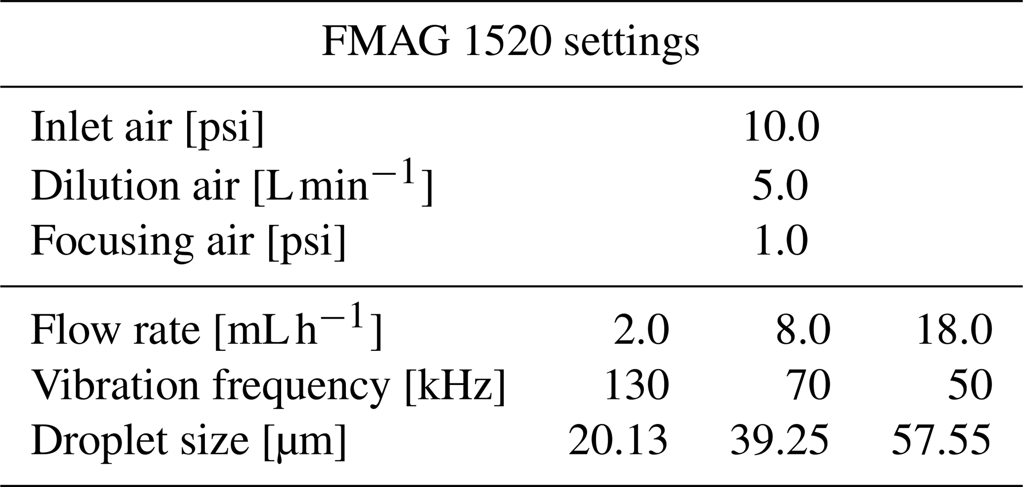
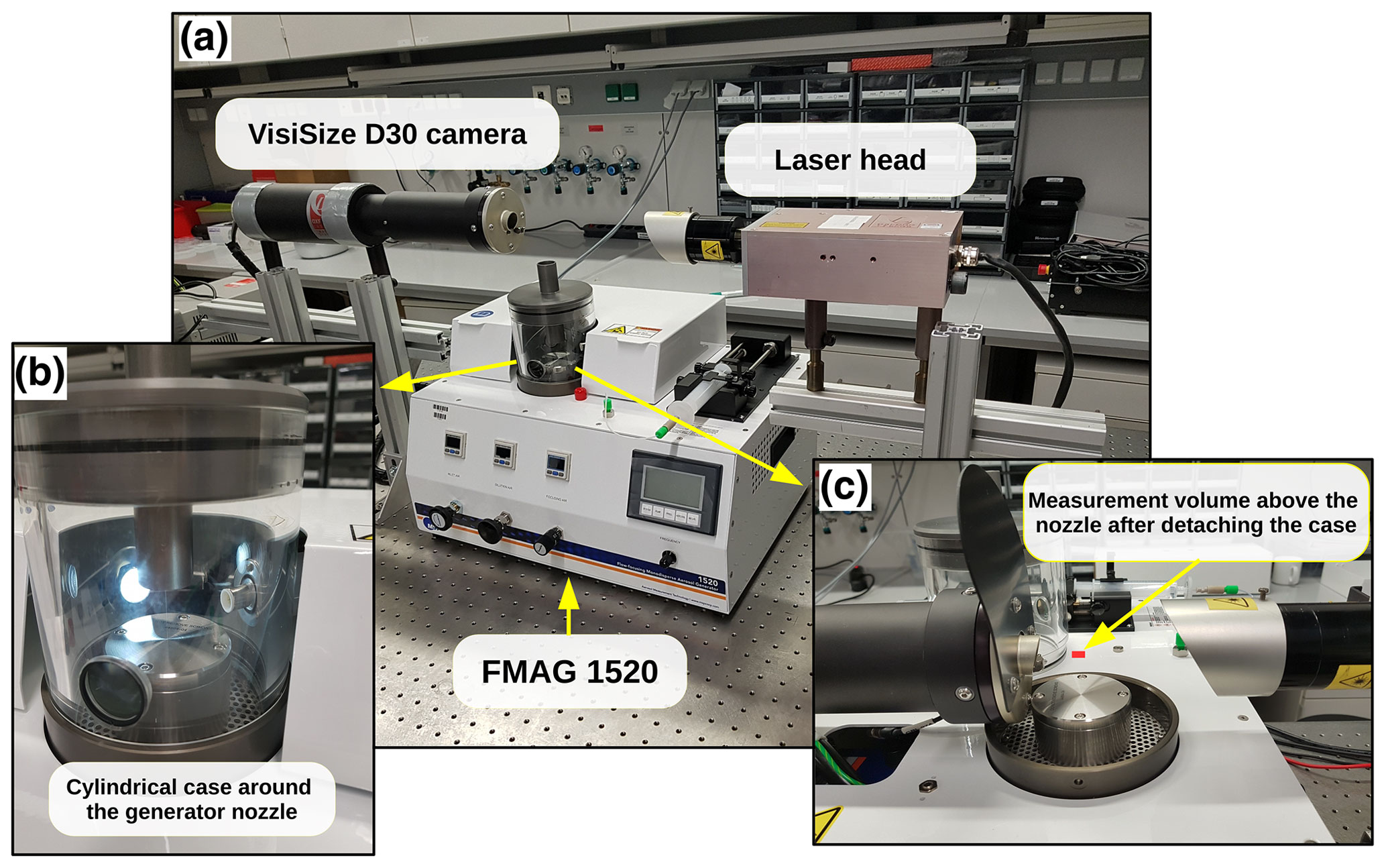
Figure 10Experimental setup for studying sizing performance. The VisiSize D30 was located above the exit of the FMAG in order to measure outgoing droplets (a) in the configuration with the cylindrical case above the nozzle (b) and in the configuration without the case (c).
4.2 Results
Sample shadow images of droplets produced by the FMAG and captured by the VisiSize D30 are reproduced in Fig. 11. The configuration of the setup was as shown in Fig. 10c, i.e. without the case covering the nozzle. Although the population of droplets was assumed to be monodisperse, a range of sizes can be seen. For each droplet size specified by the parameters of the FMAG, a series of images was taken by the shadowgraph with three different lens magnification settings. Results are presented in Fig. 12 in the form of probability density functions (PDFs, equivalent to ). This measure was chosen so that it was possible to compare DSDs for different magnifications and measurements that differed substantially in total droplet concentration, which was not a quantity of interest in the current analysis.
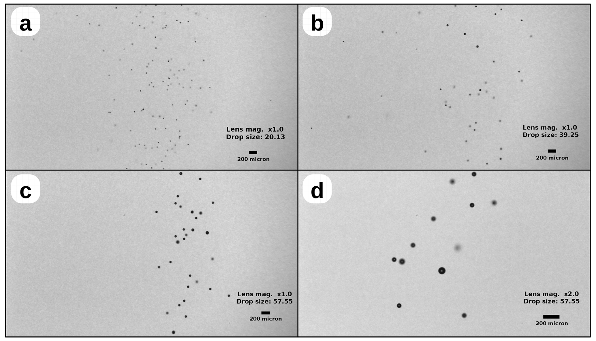
Figure 11Sample shadow images captured by the VisiSize D30, showing droplets with different sizes that were generated by the FMAG.
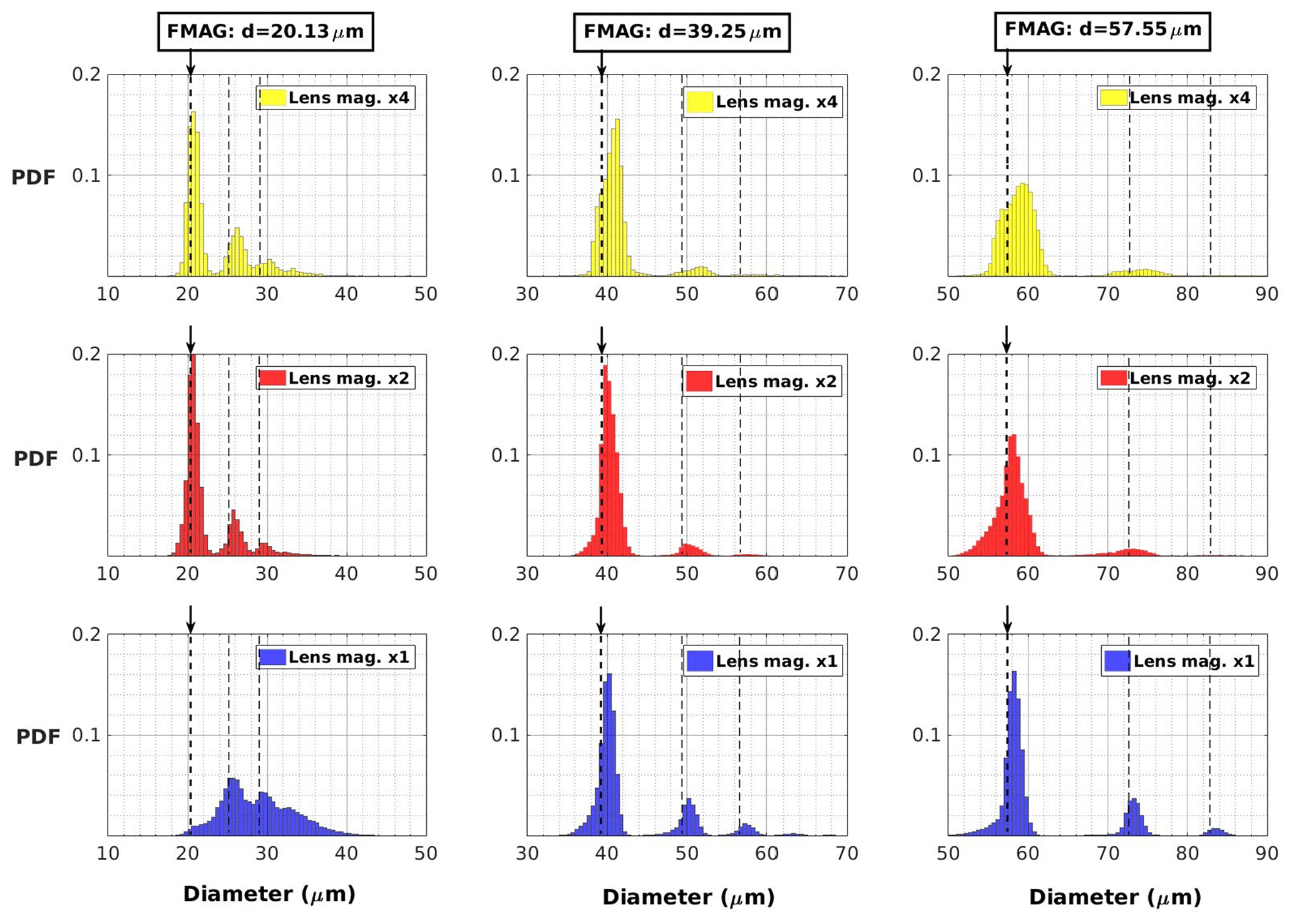
Figure 12Probability distributions of droplet size measured by the VisiSize D30 in the configuration shown in Fig. 10c (the distance between the sample volume and the nozzle head was ∼4.5 cm) for different camera lens magnifications and FMAG output droplet sizes. The initial size of the generated droplets as well as the droplet sizes after double and triple collisions are marked with vertical lines.
Strikingly, all of the histograms contain multiple peaks, which suggests that collisions between droplets on their way from the nozzle to the SV of the shadowgraph are quite frequent. The position of the first peak agrees well with the generated droplet size in most cases. The peak width can be attributed to the inevitable spread in the actual generated droplet diameters as well as the imperfect imaging and sizing of droplet shadows. The left-side skewness of the tails suggests partial evaporation. Although the effect of evaporation is generally expected to be more significant for small droplets, skewness is evident for the 39.25 and 57.55 µm droplets measured with the lens settings ×1 and ×2. We speculate that this might be related to the size of the sample volume, which increases with the effective pixel size (decreases with magnification) and the particle size (i.e. from the top-left to the bottom-right panel in Fig. 12). The position of the nozzle exit was adjusted so that the centre of the FMAG-generated droplet stream was as close as possible to the focal plane of the shadowgraph. We expect that the droplets which were more distant from the central axis of the stream were more likely to have been partially evaporated because of their longer travel times and exposure to the dry air blown from the area around the nozzle. Those droplets can be detected when the sample volume is large but not in the case of a small SV. Importantly, this is only one of the effects which could have contributed to the observed result, together with the ambient air properties, the velocity of the droplets and interactions between them.
Taking into account the geometric standard deviation of the generated droplets (1.05), the histogram bin width (0.5 µm) and evaporation, the sizing achieved by the shadowgraph is pretty accurate. The reported diameters only seem to be significantly biased for the smallest droplets (20.13 µm) and at the lowest lens magnification (×1). This issue is probably instrumental in origin and may be due to nonuniform illumination of the FOV, which also caused inhomogeneity in the detection of relatively small objects for that particular lens setting (see Sect. 3.5).
The occurrence of droplet collisions is further corroborated by measurements conducted in the configuration shown in Fig. 10b, i.e. with the cylindrical case over the nozzle, and with a long distance between the nozzle exit and the shadowgraph SV (around 18.5 cm). A long path enhances the chance of collisions and the effects of evaporation. The former can be clearly seen in the histograms presented in Fig. 13. Consecutive peaks correspond to the initially generated droplets, droplets produced in double collisions, and droplets produced in triple collisions; the positions of the vertical lines in the plot were calculated by simply summing the volumes of droplets of the size generated by the FMAG. Here, the lens magnification setting ×1 was applied as it provided the largest SV and thus the best statistics, improving the estimation of less frequent events in the probability distribution. More distant peaks can be traced best for the largest droplet size, suggesting that the probability of high-order collisions might increase with size. This is expected based on extensive studies of cloud droplet collision kernels (Devenish et al., 2012; Grabowski and Wang, 2013). Left-skewed tails are also visible, in particular for the first peak, which is a consequence of evaporation during the 18.5 cm path from the nozzle.
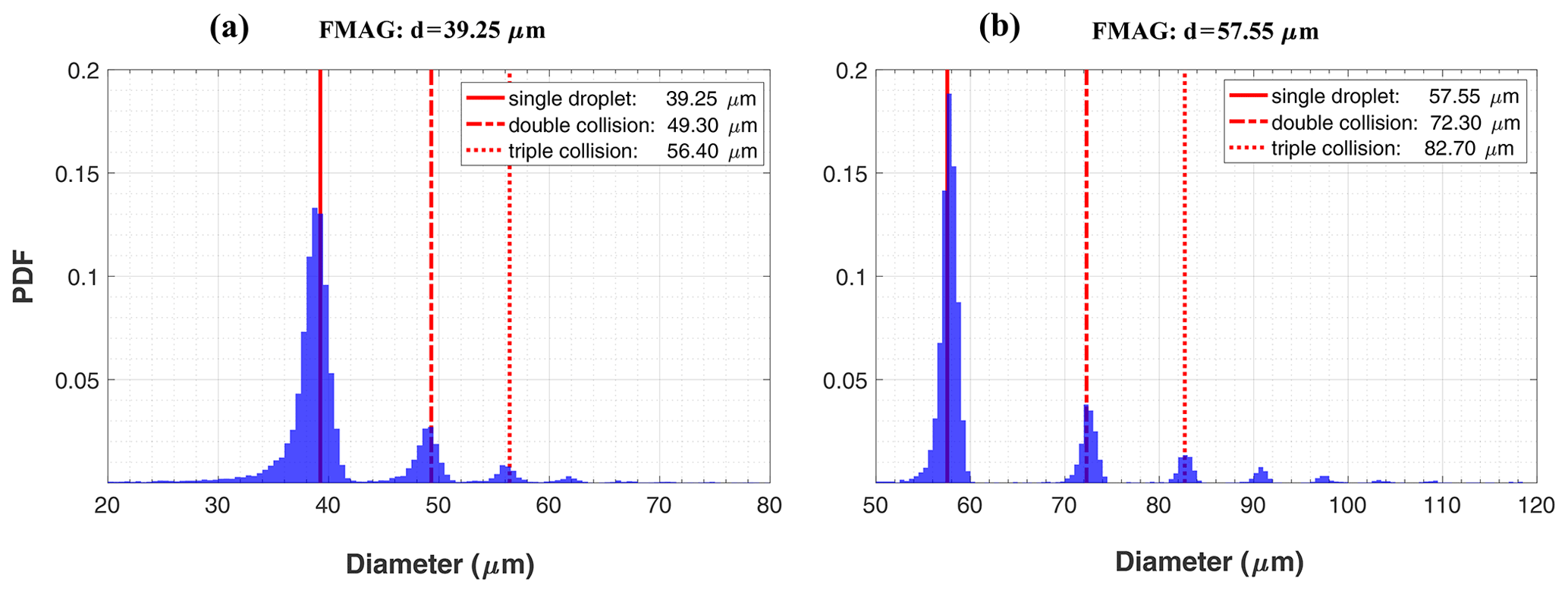
Figure 13Probability distributions of droplet size measured by the VisiSize D30 in the configuration shown in Fig. 10b (the distance between the sample volume and the nozzle head is ∼18.5 cm) for camera lens magnification setting ×1. The initial size of the generated droplets as well as the droplet sizes after double and triple collisions are marked with vertical red lines.

Figure 14Comparison of droplet sizing using the VisiSize D30 and the FMAG. Scatter plot illustrates the position of the first peak in the size histogram and the arithmetic mean diameter with respect to the FMAG-generated droplet size for different lens magnification settings (left). The red boxes (a, b, c) in the scatter plot are enlarged in the panels on the right. Each pair of points (filled and empty) represents a single measurement.
Finally, the sizing accuracy is evaluated more quantitatively in the scatter plot shown in Fig. 14, which compares the initial droplet size as specified by the FMAG with the results obtained with the shadowgraph – the mean droplet diameter reported by the software and the position of the first major peak in the size histogram. Obviously, the mean diameter is larger than the first peak as it includes the contribution from droplets that have collided. Excluding the problematic case where the magnification setting was ×1 for a size of 20.13 µm, the position of the first peak deviates by up to 2 µm from the original value, and the relative error ranges up to roughly 5 %. However, these are only estimated upper bounds on the accuracy of the shadowgraph instrument for those quantities, as the generated size is also subject to intrinsic uncertainty. Hence, based on a comparison with the FMAG, the sizing performed by the shadowgraph is indeed accurate enough apart from when small droplets are observed at magnification setting ×1. Interestingly, the first peak estimated using the shadowgraph generally occurs at a larger diameter than the FMAG-generated droplet size. Even though the opposite would be expected due to evaporation. This fact suggests that the shadowgraph slightly overestimates the sizes with respect to the FMAG-generated droplet sizes in most cases.
After laboratory tests, the shadowgraph VisiSize D30 was used for the first time to measure droplets in atmospheric clouds in order to test its performance under harsh environmental conditions, to compare it with other probes already in service in cloud physics studies, and to study microphysical properties of warm (liquid) orographic clouds. The measurements were performed at a mountain-based observatory – the Environmental Research Station (Umweltforschungsstation) Schneefernerhaus, located on the southern slope of Zugspitze in the Bavarian Alps – during two observational periods in July and August 2019. Typical meteorological conditions and cloud and turbulence properties at this location are described in detail in Siebert et al. (2015) and Risius et al. (2015).
A comprehensive analysis of the field experiment along with the results obtained with the shadowgraphy imaging technique will be provided in a separate article. Here we present examples of observations of cloud microphysical properties representing the range of conditions typical of this location. The data were collected on 13 July 2019 when cloud covered the sky for most of the day (7–8 oktas). However, due to the wind and complex terrain, the observatory is usually exposed only intermittently to cloudy air. Two measurement series, each 15 min long and recorded under relatively homogeneous conditions, were selected. The first was performed in the afternoon (14:46–15:01 LT) using lens magnification setting ×2, and the second in the late evening (23:19–23:34 LT) using ×4. Throughout the day, the temperature varied around 0 ∘C. The wind was predominantly westerly, coming over the saddle in the mountain range located west from the observatory. It was stronger for the first measurement series – around 5 m s−1, with fluctuations of 2 m s−1 – than for the second series (a mean velocity of about 1.5 m s−1 and fluctuations of 1 m s−1). No precipitation was noticed in the afternoon, whereas light rain occurred in the evening shortly before the measurement.
Figure 15 presents normalized DSDs calculated with the methods described in Sect. 3.4 for the two recorded events. Basic microphysical statistics calculated based on the DSDs are listed in Table 6. Naturally, the results for the two series cannot be directly compared as the conditions under which they were obtained were slightly different. However, the DNC as well as the mean diameter and the LWC resemble typical properties of nonprecipitating continental clouds and are close to the range of conditions reported by Siebert et al. (2015) for Schneefernerhaus Observatory based on measurements taken with a completely different instrument (PDI).
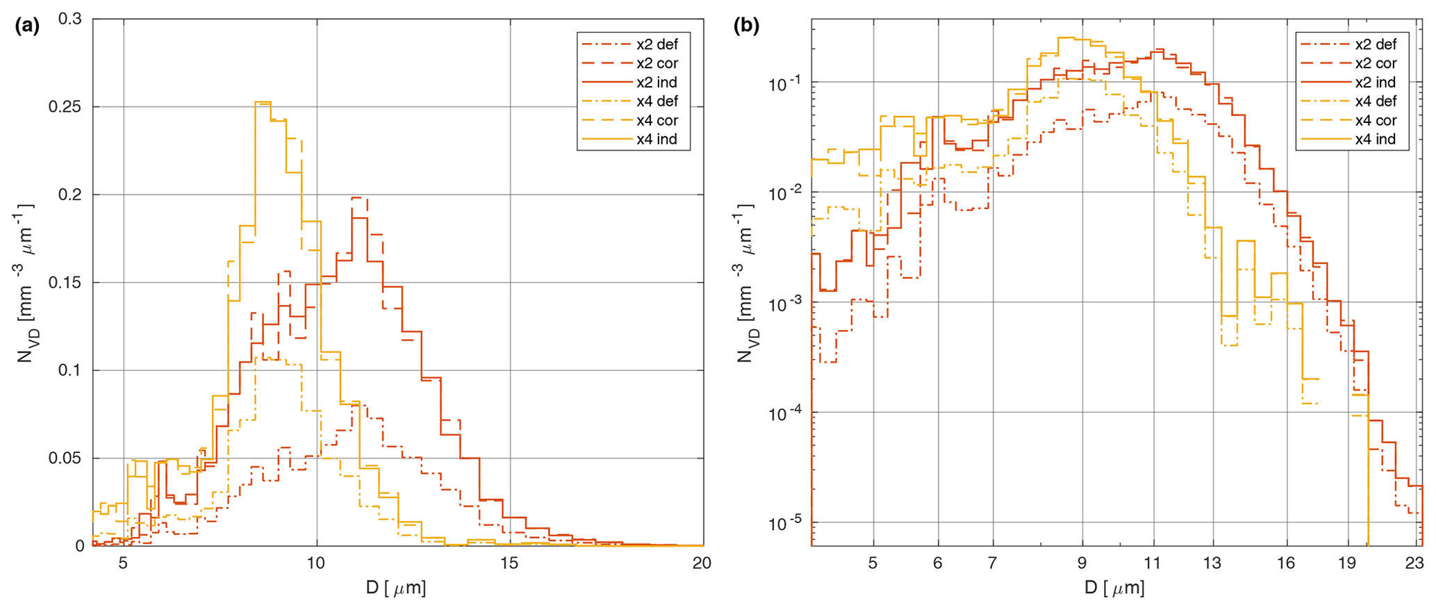
Figure 15Droplet size distributions in clouds observed with the VisiSize D30 at Schneefernerhaus Observatory during two events on 13 July 2019: one in the afternoon (14:46–15:01 LT) and the other in the late evening (23:19–23:34 LT), the former taken with lens setting ×2 and the latter with setting ×4. Three methods of calculating the results – default (def), corrected (cor) and individual (ind) (see Sect. 3.4 for explanations) – are indicated by different line styles. The same data are plotted on (a) linear and (b) logarithmic scales.
Table 6Results of the cloud observations performed with the VisiSize D30 at Schneefernerhaus on 13 July 2019.
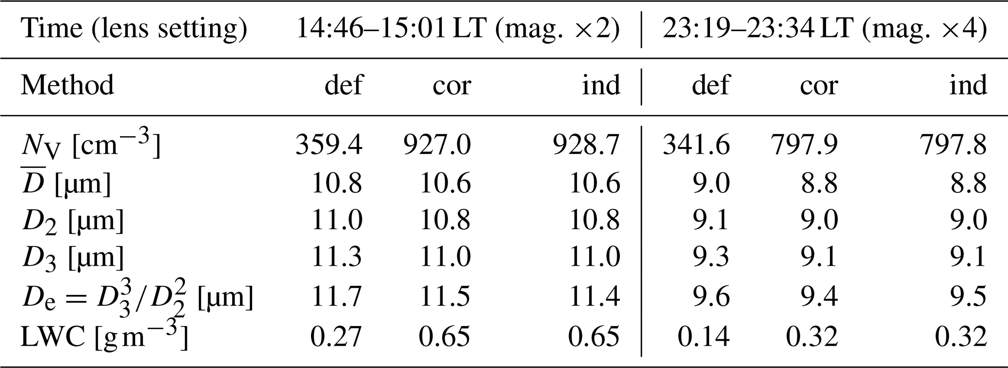
The cloud observed in the afternoon seems to have contained a greater fraction of larger droplets (10–15 µm) than the cloud in the evening. In both cases, however, the droplets were produced mostly by condensation, as the maximum diameters measured do not correspond to the sizes yielded by efficient collision-induced rain formation. It should be noted that the moments of the DSD (mean diameter statistics) are most probably moderately overestimated because the proportion of small droplets throughout the whole relevant volume may not have been properly determined. The minimum diameter required for uniform reliable detection was estimated to be ∼6 µm for lens setting ×2 (see Sect. 3.4), but was unfortunately not determined precisely for lens setting ×4 (although it was definitely between 2 and 6 µm). Obviously, the degree of bias decreases with the magnification (improving resolution). For the same reason, the total DNC might be moderately underestimated compared to the actual value. Nevertheless, all of the instruments suffer from similar issues whenever the range of detectable diameters is finite. The relative differences between the three methods of calculating the DSD are very similar to those stated for the laboratory experiment (Sect. 3.4).
The comparison between the two example observations discussed in this section also illustrates the trade-off regarding the choice of magnification. Greater magnification (setting ×4) provides better resolution and proper representation of the left tail of the DSD (below 6 µm), though the right tail – corresponding to relatively scarce large droplets – is then poorly represented statistically because the total number of counts is quite modest. Specifically, despite the similar DNCs and measurement durations of the two series, roughly 10 times more droplets were recorded in the first series (×2), simply due to the larger SV.
A shadowgraph imaging system – the Oxford Lasers VisiSize D30 – has been tested and characterized through application to cloud microphysical measurements, i.e. the number concentration and size of cloud droplets. The instrument captures images containing shadows of multiple particles, counts them, and estimates particle sizes while correcting for image blurring due to out-of-focus particle positions. Although developed for industrial applications, the system can be applied for cloud physics studies. Nevertheless, diagnostic laboratory experiments have highlighted important limitations which need to be considered.
First, the sample volume within which a droplet is detectable depends on the size of the droplet because blurring caused by defocus affects images of particles with different sizes differently. This fact must always be taken into account when estimating the droplet concentration (in a unit volume). The solution implemented in the software assumes a linear relation between depth of field and particle diameter which is efficient for relatively large objects (>260 µm; the exact value depends on the lens magnification). However, for small droplets such as those in clouds, the additional focus rejection criterion imposes a much stronger limit on the acceptable depth of field. This affects the relevant sample volume and leads to an underestimated number concentration. Therefore, we developed a correction method using the sample volume based on that limit.
Second, an analysis of detections in a dense polydisperse stream of droplets implied that the minimum droplet size for reliably uniform detection is significantly larger than the resolution in the focal plane. This minimum droplet size was estimated to be ∼6 and ∼12 µm for the camera lens magnification settings ×2 and ×1, respectively. It can potentially be enhanced by careful data conditioning, i.e. with a strong limit on the estimated distance from the focal plane, but at the cost of decreasing the sample volume. Furthermore, detection probability was found to be satisfactorily homogeneous across the field of view, except for the small magnification setting (×1). Minor issues with respect to the axial direction were revealed, which were probably caused by substantial diffraction effects on small droplets.
Third, a test of sizing accuracy was performed using a monodisperse droplet generator (FMAG 1520, TSI). Substantial effects of droplet collisions and evaporation were observed in the size histograms obtained with the shadowgraph. Notwithstanding, after filtering out collisions by selecting the first major peak, the results indicated reasonable agreement between the diameters reported by the shadowgraph and those assumed to be generated by the FMAG. The difference was no larger than 2 µm or 5 %, again except at the lens magnification setting ×1, for which uniform illumination of the scene proved difficult.
Finally, the system under study was applied to sample atmospheric clouds in a ground-based mountain observatory. It performed satisfactorily under windy, cloudy, humid weather conditions and provided an extensive set of microphysical data which will be presented and discussed in detail in a separate publication. The results of the selected observations analysed here comply with the expected conditions and previous independent measurements performed at that location.
To sum up, the VisiSize D30 can be successfully applied for cloud microphysical measurements. However, relevant quantities such as droplet size distribution, number concentration, mean diameter or effective diameter need to be calculated with care, accounting for the size-dependent sample volume. While conducting the experiment, one should adjust the laser and the camera appropriately to ensure uniform illumination of the field of view. We recommend avoiding low magnification settings (e.g. ×1) as they make it difficult to properly adjust the illumination and are of limited utility for cloud studies due to the high minimum diameter for satisfactory detection. Those settings might instead be advantageous for sampling drizzle and rain, which is a topic that is currently being studied.
The results presented in this study were obtained with the use of the Oxford Lasers VisiSize software version 6.5.39 and the codes developed by the authors in MATLAB environment. The latter are available from the authors upon request.
The data presented in this study is available from the authors upon request.
JLN, MM and SPM designed the study. JLN planned and carried out the detection experiment (Sect. 3). MM planned and carried out the sizing experiment (Sect. 4). MM carried out the field experiment, while MM and JLN analysed the collected data. JLN and MM wrote the manuscript with contributions from SPM.
The authors declare that they have no conflict of interest.
We thank Gholamhossein Bagheri, Jan Molacek and the staff of the Max Planck Institute for Dynamics and Self-Organization (MPIDS) for providing the FMAG aerosol generator and their help during the laboratory sizing experiments in Göttingen. We are also grateful to Till Rehm and the staff of the Umweltforschungsstation Schneefernerhaus (UFS) for their help during the field measurements at Mt. Zugspitze. Special appreciation is extended to Wojciech Kumala for providing technical support during the laboratory detection experiments in Warsaw.
This research has been supported by the European Union's Horizon 2020 research and innovation programme under the Marie Skłodowska-Curie Actions (COMPLETE (grant agreement no. 675675)).
This paper was edited by Zamin A. Kanji and reviewed by two anonymous referees.
Bachalo, W. D. and Houser, M. J.: Phase/Doppler Spray Analyzer For Simultaneous Measurements Of Drop Size And Velocity Distributions, Opt. Eng., 23, 235583, https://doi.org/10.1117/12.7973341, 1984. a
Barone, T. L., Hesse, E., Seaman, C. E., Baran, A. J., Beck, T. W., Harris, M. L., Jaques, P. A., Lee, T., and Mischler, S. E.: Calibration of the cloud and aerosol spectrometer for coal dust composition and morphology, Advanced Powder Technol., 30, 1805–1814, https://doi.org/10.1016/j.apt.2019.05.023, 2019. a
Beck, A., Henneberger, J., Schöpfer, S., Fugal, J., and Lohmann, U.: HoloGondel: in situ cloud observations on a cable car in the Swiss Alps using a holographic imager, Atmos. Meas. Tech., 10, 459–476, https://doi.org/10.5194/amt-10-459-2017, 2017. a
Bewley, G. P., Saw, E. W., and Bodenschatz, E.: Observation of the sling effect, New J. Phys., 15, 083051, https://doi.org/10.1088/1367-2630/15/8/083051, 2013. a
Bordás, R., Roloff, C., Thévenin, D., and Shaw, R. A.: Experimental determination of droplet collision rates in turbulence, New J. Phys., 15, 045010, https://doi.org/10.1088/1367-2630/15/4/045010, 2013. a
Brenguier, J. L., Bourrianne, T., De Coelho, A. A., Isbert, J., Peytavi, R., Trevarin, D., and Weschler, P.: Improvements of droplet size distribution measurements with the fast-FSSP (Forward Scattering Spectrometer Probe), J. Atmos. Ocean. Tech., 15, 1077–1090, https://doi.org/10.1175/1520-0426(1998), 1998. a
Chuang, P. Y., Saw, E. W., Small, J. D., Shaw, R. A., Sipperley, C. M., Payne, G. A., and Bachalo, W. D.: Airborne Phase Doppler Interferometry for Cloud Microphysical Measurements, Aerosol Sci. Tech., 42, 685–703, https://doi.org/10.1080/02786820802232956, 2008. a
Connolly, P. J., Flynn, M. J., Ulanowski, Z., Choularton, T. W., Gallagher, M. W., and Bower, K. N.: Calibration of the cloud particle imager probes using calibration beads and ice crystal analogs: The depth of field, J. Atmos. Ocean. Tech., 24, 1860–1879, https://doi.org/10.1175/JTECH2096.1, 2007. a
Cooper, W. A.: Effects of Coincidence on Measurements with a Forward Scattering Spectrometer Probe, J. Atmos. Ocean. Tech., 5, 823–832, https://doi.org/10.1175/1520-0426(1988), 1988. a
de Araújo Coelho, A., Brenguier, J. L., and Perrin, T.: Droplet spectra measurements with the FSSP-100, Part I: Low droplet concentration measurements, J. Atmos. Ocean. Tech., 22, 1748–1755, https://doi.org/10.1175/JTECH1817.1, 2005. a
Devenish, B. J., Bartello, P., Brenguier, J. L., Collins, L. R., Grabowski, W. W., Ijzermans, R. H., Malinowski, S. P., Reeks, M. W., Vassilicos, J. C., Wang, L. P., and Warhaft, Z.: Droplet growth in warm turbulent clouds, Q. J. Roy. Meteor. Soc., 138, 1401–1429, https://doi.org/10.1002/qj.1897, 2012. a, b
Duan, H., Romay, F. J., Li, C., Naqwi, A., Deng, W., and Liu, B. Y. H.: Generation of monodisperse aerosols by combining aerodynamic flow-focusing and mechanical perturbation, Aerosol Sci. Tech., 50, 17–25, https://doi.org/10.1080/02786826.2015.1123213, 2016. a, b
Fugal, J. P. and Shaw, R. A.: Cloud particle size distributions measured with an airborne digital in-line holographic instrument, Atmos. Meas. Tech., 2, 259–271, https://doi.org/10.5194/amt-2-259-2009, 2009. a
Fugal, J. P., Schulz, T. J., and Shaw, R. A.: Practical methods for automated reconstruction and characterization of particles in digital in-line holograms, Meas. Sci. Technol., 20, 75501, https://doi.org/10.1088/0957-0233/20/7/075501, 2009. a
Gerber, H., Frick, G., and Rodi, A. R.: Ground-based FSSP and PVM measurements of liquid water content, J. Atmos. Ocean. Tech., 16, 1143–1149, https://doi.org/10.1175/1520-0426(1999), 1999. a
Glen, A. and Brooks, S. D.: A new method for measuring optical scattering properties of atmospherically relevant dusts using the Cloud and Aerosol Spectrometer with Polarization (CASPOL), Atmos. Chem. Phys., 13, 1345–1356, https://doi.org/10.5194/acp-13-1345-2013, 2013. a
Grabowski, W. W. and Wang, L.-P.: Growth of Cloud Droplets in a Turbulent Environment, Annu. Rev. Fluid Mech., 45, 293–324, https://doi.org/10.1146/annurev-fluid-011212-140750, 2013. a
Henneberger, J., Fugal, J. P., Stetzer, O., and Lohmann, U.: HOLIMO II: a digital holographic instrument for ground-based in situ observations of microphysical properties of mixed-phase clouds, Atmos. Meas. Tech., 6, 2975–2987, https://doi.org/10.5194/amt-6-2975-2013, 2013. a
Kashdan, J. T., Shrimpton, J. S., and Whybrew, A.: Two-Phase Flow Characterization by Automated Digital Image Analysis, Part 1: Fundamental Principles and Calibration of the Technique, Part. Part. Syst. Char., 20, 387–397, https://doi.org/10.1002/ppsc.200300897, 2003. a, b, c, d, e
Kashdan, J. T., Shrimpton, J. S., and Whybrew, A.: Two-Phase Flow Characterization by Automated Digital Image Analysis, Part 2: Application of PDIA for Sizing Sprays, Part. Part. Syst. Char., 21, 15–23, https://doi.org/10.1002/ppsc.200400898, 2004. a, b
Korczyk, P. M., Kowalewski, T. A., and Malinowski, S. P.: Turbulent mixing of clouds with the environment: Small scale two phase evaporating flow investigated in a laboratory by particle image velocimetry, Physica D, 241, 288–296, https://doi.org/10.1016/j.physd.2011.11.003, 2012. a
Kumar, M. S., Chakravarthy, S. R., and Mathur, M.: Optimum air turbulence intensity for polydisperse droplet size growth, Physical Review Fluids, 4, 074607, https://doi.org/10.1103/PhysRevFluids.4.074607, 2019. a
Lance, S.: Coincidence errors in a cloud droplet probe (CDP) and a cloud and aerosol spectrometer (CAS), and the improved performance of a modified CDP, J. Atmos. Ocean. Tech., 29, 1532–1541, https://doi.org/10.1175/JTECH-D-11-00208.1, 2012. a, b
Lance, S., Brock, C. A., Rogers, D., and Gordon, J. A.: Water droplet calibration of the Cloud Droplet Probe (CDP) and in-flight performance in liquid, ice and mixed-phase clouds during ARCPAC, Atmos. Meas. Tech., 3, 1683–1706, https://doi.org/10.5194/amt-3-1683-2010, 2010. a
Larsen, M. L. and Shaw, R. A.: A method for computing the three-dimensional radial distribution function of cloud particles from holographic images, Atmos. Meas. Tech., 11, 4261–4272, https://doi.org/10.5194/amt-11-4261-2018, 2018. a
Lawson, R. P., Baker, B. A., Schmitt, C. G., and Jensen, T. L.: An overview of microphysical properties of Arctic clouds observed in May and July 1998 during FIRE ACE, J. Geophys. Res., 106, 14989–15014, https://doi.org/10.1029/2000JD900789, 2001. a
Lloyd, G., Choularton, T., Bower, K., Crosier, J., Gallagher, M., Flynn, M., Dorsey, J., Liu, D., Taylor, J. W., Schlenczek, O., Fugal, J., Borrmann, S., Cotton, R., Field, P., and Blyth, A.: Small ice particles at slightly supercooled temperatures in tropical maritime convection, Atmos. Chem. Phys., 20, 3895–3904, https://doi.org/10.5194/acp-20-3895-2020, 2020. a
McFarquhar, G. M., Um, J., Freer, M., Baumgardner, D., Kok, G. L., and Mace, G.: Importance of small ice crystals to cirrus properties: Observations from the Tropical Warm Pool International Cloud Experiment (TWP-ICE), Geophys. Res. Lett., 34, L13803, https://doi.org/10.1029/2007GL029865, 2007. a
Ramelli, F., Beck, A., Henneberger, J., and Lohmann, U.: Using a holographic imager on a tethered balloon system for microphysical observations of boundary layer clouds, Atmos. Meas. Tech., 13, 925–939, https://doi.org/10.5194/amt-13-925-2020, 2020. a
Risius, S., Xu, H., Di Lorenzo, F., Xi, H., Siebert, H., Shaw, R. A., and Bodenschatz, E.: Schneefernerhaus as a mountain research station for clouds and turbulence, Atmos. Meas. Tech., 8, 3209–3218, https://doi.org/10.5194/amt-8-3209-2015, 2015. a
Rydblom, S. and Thörnberg, B.: Liquid water content and droplet sizing shadowgraph measuring system for wind turbine icing detection, IEEE Sens. J., 16, 2714–2725, https://doi.org/10.1109/JSEN.2016.2518653, 2016. a
Schlenczek, O.: Airborne and ground-based holographic measurement of hydrometeors in liquid-phase, mixed-phase and ice clouds, PhD thesis, Johannes Gutenberg University in Mainz, Germany, 316 pp., https://doi.org/10.25358/openscience-4124, 2017a. a
Schlenczek, O., Fugal, J. P., Lloyd, G., Bower, K. N., Choularton, T. W., Flynn, M., Crosier, J., and Borrmann, S.: Microphysical Properties of Ice Crystal Precipitation and Surface-Generated Ice Crystals in a High Alpine Environment in Switzerland, J. Appl. Meteorol. Clim., 56, 433–453, https://doi.org/10.1175/JAMC-D-16-0060.1, 2017b. a
Siebert, H., Shaw, R. A., Ditas, J., Schmeissner, T., Malinowski, S. P., Bodenschatz, E., and Xu, H.: High-resolution measurement of cloud microphysics and turbulence at a mountaintop station, Atmos. Meas. Tech., 8, 3219–3228, https://doi.org/10.5194/amt-8-3219-2015, 2015. a, b
Woods, S., Lawson, R. P., Jensen, E., Bui, T. P., Thornberry, T., Rollins, A., Pfister, L., and Avery, M.: Microphysical Properties of Tropical Tropopause Layer Cirrus, J. Geophys. Res.-Atmos., 123, 6053–6069, https://doi.org/10.1029/2017JD028068, 2018. a