Study on the measurement of isoprene by differential optical absorption spectroscopy

In this paper, the continuous online measurements of isoprene in the atmosphere have been carried out by using differential optical absorption spectroscopy (DOAS) in the band of 202.71–227.72 nm for the first time. Under a zero optical path in the laboratory, different equivalent concentrations of isoprene were measured by the combination of known concentrations of gas and series calibration cells. The correlation between the measured concentrations and the equivalent concentrations was 0.9995, and the slope was 1.065. The correlation coefficient between DOAS and the online volatile organic compound (VOC) instrument observed from 23 d of field observations is 0.85 with a slope of 0.86. It was estimated that the detection limit of isoprene with DOAS is approximately 0.1 ppb at an optical path of 75 m, and it was verified that isoprene could be measured in the ultraviolet absorption band using the DOAS method with high temporal resolution and a low maintenance cost.

1 Introduction

Isoprene, named as 2-methyl-1,3-butadiene (C₅H₈), is an important BVOC (biogenic volatile organic compound) in the atmosphere. Its global emission rate is about 500 Tg C yr⁻¹ (Sindelarova et al., 2014). Isoprene accounts for 70 % of global BVOC emissions (Aydin et al., 2014). Land vegetation and other natural sources contribute 90 % of isoprene in the atmosphere (Zhang et al., 2016), and anthropogenic emissions mainly come from industrial activities. Isoprene, as a typical pentadiene hydrocarbon, has a higher activity than ordinary anthropogenic VOCs (Lian et al., 2020), and its lifetime in the boundary layer is only about half an hour (Zheng et al., 2015). Due to high volatility and reaction activity, isoprene can accelerate the reaction between atmospheric substances, and it easily reacts with strong oxidizing substances (OH, NO₃ radicals, etc.) and also affects the balance between NO_x (NO_x = NO + NO₂) and O₃ in the atmosphere. Isoprene is also the precursor of secondary organic aerosol (SOA) (Zeng et al., 2018).

Isoprene produced by plants is a byproduct of photosynthesis; its emission intensity directly relates to the abundance of plants, leaf area index and plant species. Meteorological parameters, such as temperature, radiation intensity and humidity, can also affect isoprene emissions (Bai, 2015). In the daytime, the chemical process oxidized by OH is the main sink of isoprene. Due to the existence of multiple double bonds, the additional reaction with OH will lead to the formation of a variety of products and the formation of RO₂. In the presence of NO_x, RO₂ can be further reacted to convert RO and HO₂, causing the mutual conversion of free radicals and the accumulation of ozone, which affects the balance of O₃ in the atmosphere (Chen et al., 2020; Lu et al., 2018; Zhu et al., 2020). Meanwhile, the reaction of isoprene with NO₃ mainly occurs at night. Although the reaction only accounts for 6 %–7 % of the total isoprene oxidation, it is an important way to remove NO₃ (Xie et al., 2013).

In recent years, with the increase in urban vegetation diversity, the emission intensity of urban BVOCs has shown a significant upward trend. The monitoring and control of isoprene in urban ecosystems have also attracted increasing attention. Because the isoprene concentration in the atmosphere is low and its lifetime is short, highly precise and accurate methods are needed for monitoring. Currently, general methods, including gas chromatography–mass spectrometry (GC-MS), proton transfer reaction mass spectrometry (PTR-MS), and chemical ionization mass spectrometry (CIMS), have been introduced to measure isoprene.

GC-MS utilizes the high separation ability of gas chromatography to separate the components of environmental samples and then measures the different compounds with the mass spectrometer. With the advantages of high precision and stability, GC-MS can distinguish most VOCs qualitatively and quantitatively; however, it is difficult to maintain and operate due to the complex requirements of power, temperature control and special carrier gas. GC-MS measurement generally requires sampling, preservation and pre-treatment before analysis. During this process, the sample may change to some extent, resulting in inaccurate results.

PTR-MS involves the chemical ionization of a gas sample through proton transfer in a drift tube. The proton source is usually H₃O⁺. The fixed length of the drift tube provides a fixed reaction time for the ions as they move along the drift tube. The sample air is continuously pumped through the drift tube, and the VOCs in the sample react with H₃O⁺ to be ionized and then enter the mass spectrometer to be detected. The disadvantage of PTR-MS is that it completely relies on mass spectrometry to provide the identification of mixtures. VOCs are a class of substances; it is possible to have the same molecular weight or the same mass of fragment ions and parent ions. In this case, it is difficult to determine all species present and their respective concentrations. A solution to this is to combine GC with PTR-MS (Blake et al., 2009).

Table 1 Comparison of different online methods for isoprene measurement.

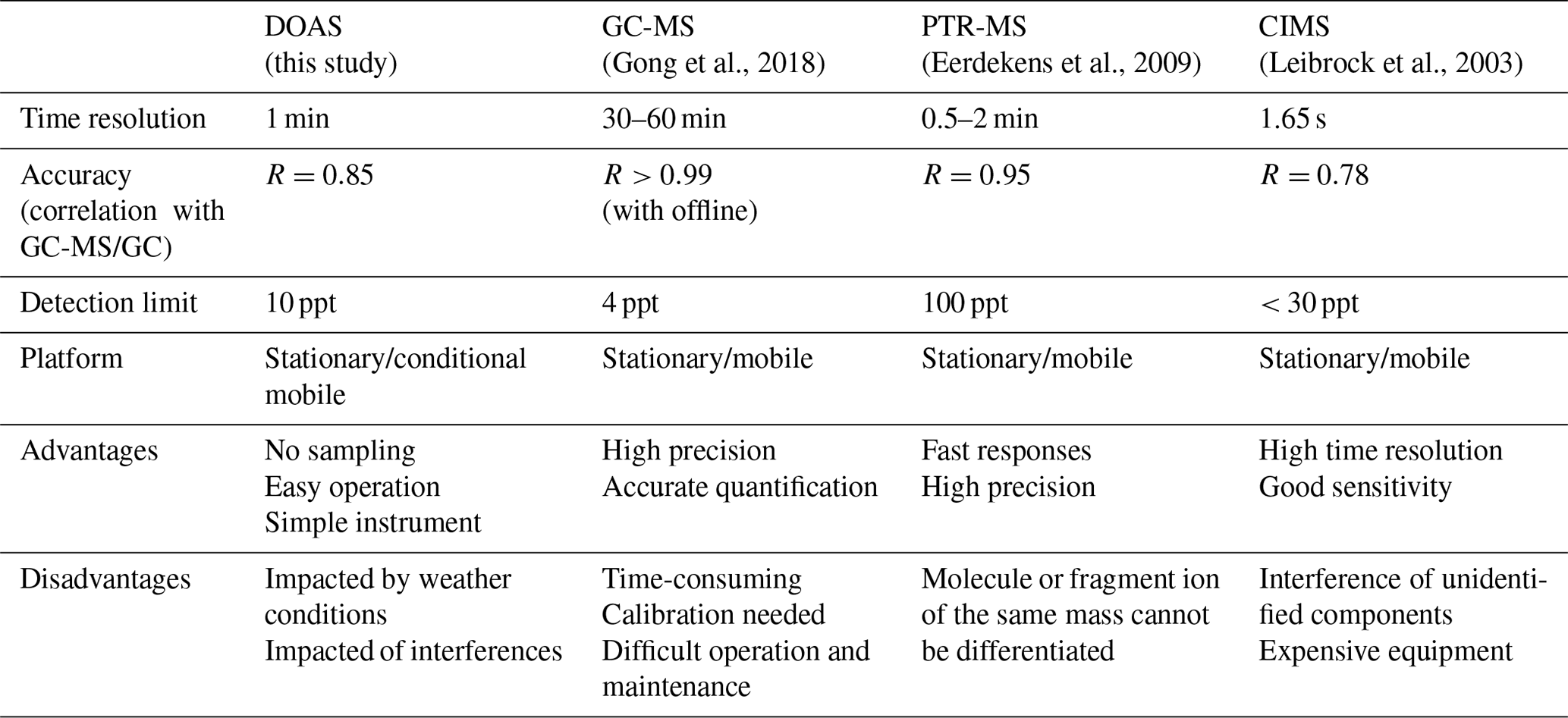
CIMS (Leibrock and Huey, 2000) retains the qualitative ability of mass spectrometry and couples the traditional air sampler with mass spectrometry technology. However, this method is not sensitive to low concentrations of isoprene. In addition, the VOC composition in the atmosphere is complex, and an unknown composition may react with the benzene reagent to interfere with the measurement results. Table 1 lists the comparison of the performance of these three methods for isoprene measurements together with the differential optical absorption spectroscopy (DOAS) method in this study.

In addition, a portable gas chromatograph (iDirac) equipped with a photo-ionization detector to measure isoprene was proposed by Bolas et al. (2020) at Cambridge University. The instrument is an improved technology for GC-MS that can work independently for weeks to months in the field environment. Previous studies have rarely mentioned the measurement of isoprene by spectral methods. Brauer et al. (2014) measured the infrared spectrum of isoprene by Fourier transform spectrometer and found that isoprene has a strong absorption near 11 000 nm, which provides a new possibility for the measurement of isoprene by spectral technology. So far, however, few people have mentioned the measurement of isoprene by ultraviolet spectroscopy. In this paper, an online measurement method with high temporal resolution for isoprene in the atmosphere is proposed by using DOAS technology in the far ultraviolet band.

2 Measurement method

2.1 Instrument introduction and spectral analysis

DOAS technology was initially proposed by Platt et al. (1979, 1980) in the 1970s. The principle of the instrument has been detailed in other literature (Platt and Stutz, 2008), so the following is a description of deep UV-DOAS. The system is mainly composed of a light source, transmitting telescope, receiving telescope, spectroscope, and computer, etc. (see Fig. 2). The transmitting and receiving telescopes are located at both ends of the measuring optical path with a distance of 75 m. Since the measurement of isoprene detects the absorption in deep ultraviolet light, we choose a deuterium lamp (L6311-50, Hamamatsu, 35 W) as the light source. The aperture of the transmitting telescope is 76 mm, with a UV-enhanced spherical mirror with a focal length of 304 mm. The aperture of the receiving telescope is 152 mm with a UV-enhanced spherical mirror with a focal length of 608 mm. A spectroscope (B&W TEK Inc. BRC741E-1024) with a spectral range of 185–400 nm, a spectral resolution of 0.75 nm FWHM (full width at half maximum), and a 1024-pixel photodiode array was used as the detector to record the spectrum. In the measurement routine, the light emitted by the light source is collimated by the transmitting telescope and then sent out. After a certain distance of transmission, it is collected by the receiving telescope and focused on the incident end of the optical fiber. The optical fiber feeds the light into the spectroscope, which detects the light signal and sends it to the computer for spectral analysis.

The measured atmospheric spectrum contains the absorption information of molecules in the atmosphere. After removing the Rayleigh scattering and Mie scattering, as well as the broadband absorption of molecules by high-pass filtering, the so-called differential absorption spectrum is obtained. This high-pass filtering is performed by a high-pass binomial on the spectrum using the 500 iterations twice to eliminate the broadband structures. The concentration of the corresponding atmospheric components can be retrieved by fitting the differential absorption spectrum with the differential absorption cross section of the measured molecules. The reference spectrum during laboratory experiments was recorded by receiving a light beam close to the transmitting device, suggesting a zero light path and no absorption of isoprene. In the field measurements, the measured atmospheric spectrum collected at 00:00 LT on 1 July 2018 was used as the reference spectrum considering it is “clean” without isoprene absorption.

Isoprene has strong absorptions between 200.0–225.0 nm, among which there are relatively obvious absorption peaks (Martins et al., 2009) near 210.0, 216.0 and 222.1 nm, as shown in Fig. 1a. After high-pass filtering, the differential absorption spectrum (1 ppb km) of isoprene is shown in Fig. 1b. According to its differential absorption characteristics, the fitting band of isoprene is 202.71–227.72 nm. Within this band, there are also absorptions of NH₃ (Chen et al., 1999), SO₂ (Wu et al., 2000), NO, NO₂ (Mérienne et al., 1995), C₆H₆ (Dawes et al., 2017), C₇H₈ (Serralheiro et al., 2015), etc. These high-resolution absorption cross sections are convoluted with the instrumental wavelength before being introduced into the spectral fitting. The absorption of NO used here was measured in the laboratory with known concentrations of gas by using the same instrument. Therefore, the absorption of these components is also considered in the process of spectral retrieval. Figure 2 displays an example of the spectral fitting of an actual atmospheric spectrum (measured on 8 July 2018 at 12:47 LT). In Fig. 2a, the black line is the measured spectrum, and the red line is the fitting spectrum (0.79 ppb isoprene, 2.83 ppb NH₃, 1.85 ppb SO₂, 1.42 ppb NO, 4.94 ppb NO₂, 0.01 ppb C₆H₆, 2.20 ppb C₇H₈), while the fitting residual (standard deviation is 4.76 × 10⁻⁴) is shown in Fig. 2i. The differential optical densities of isoprene and other interference trace gases are displayed in Fig. 2b to h, respectively, of which the measurement error of isoprene is about 10.6 % according to the method proposed by Stutz and Platt (1996).

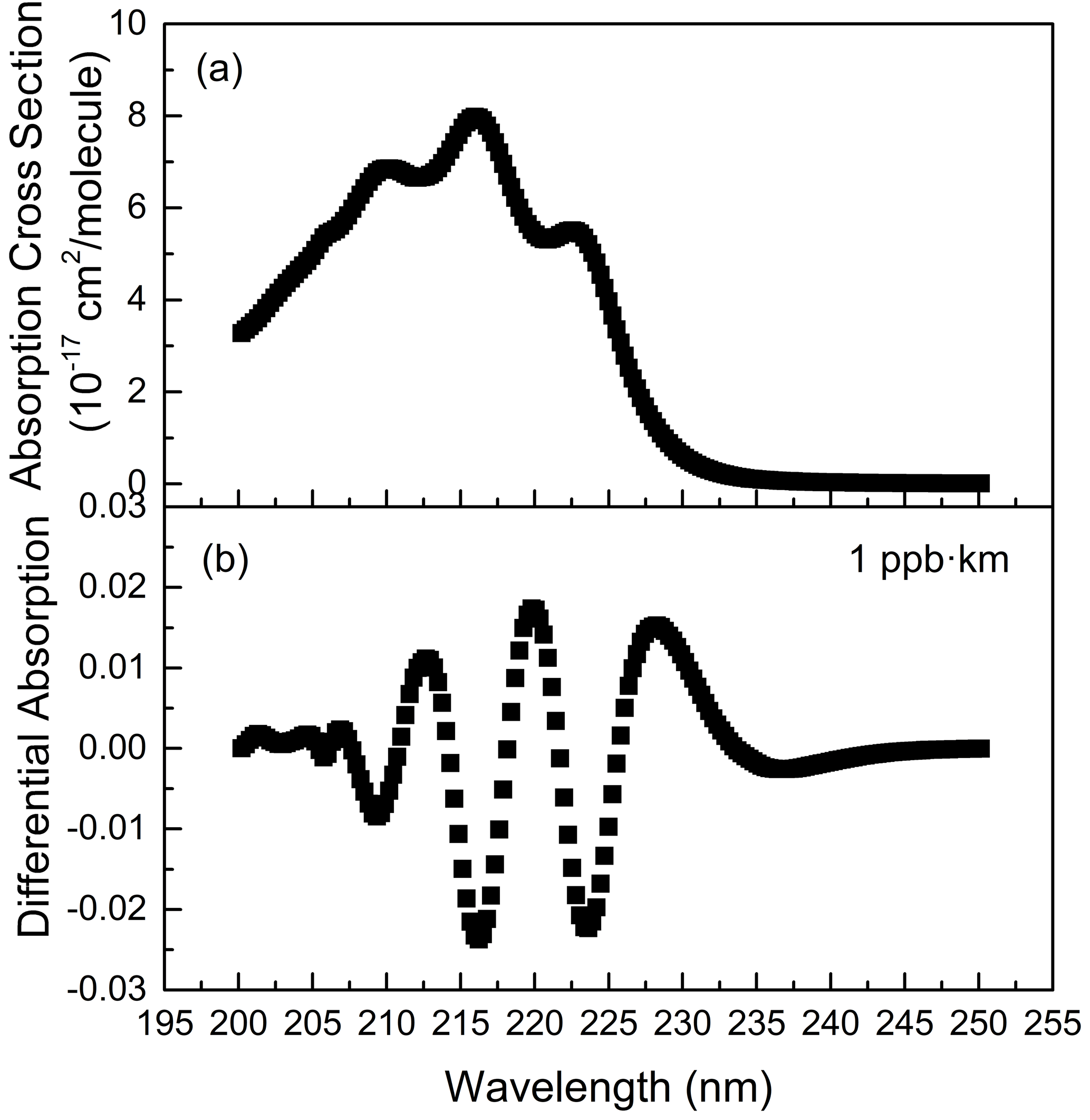
Figure 1 The absorption cross section and differential absorption spectrum of isoprene in 1 ppb km.

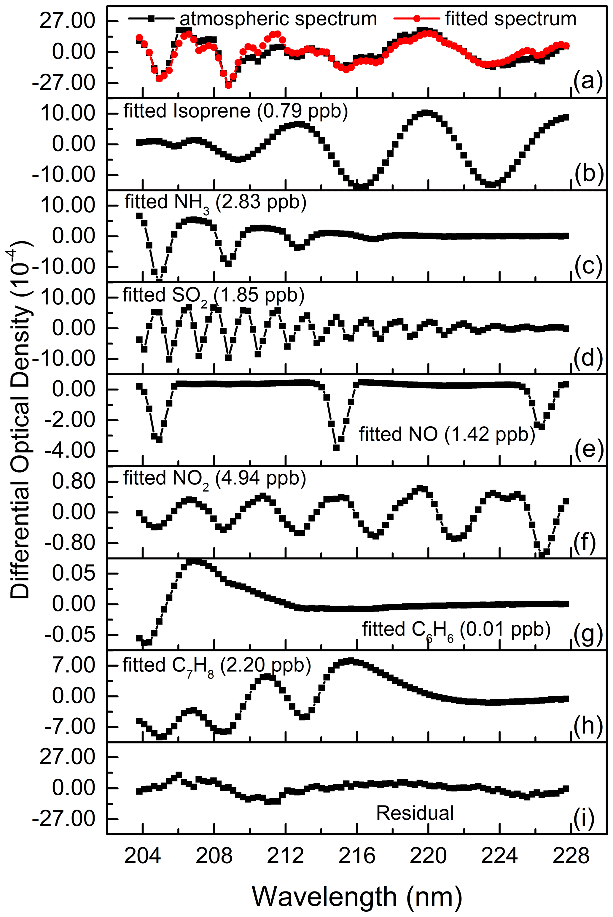
Figure 2 Example of the spectral fitting of an actual atmospheric spectrum (measured on 8 July 2018 at 12:47 LT).

2.2 Calibration experiment

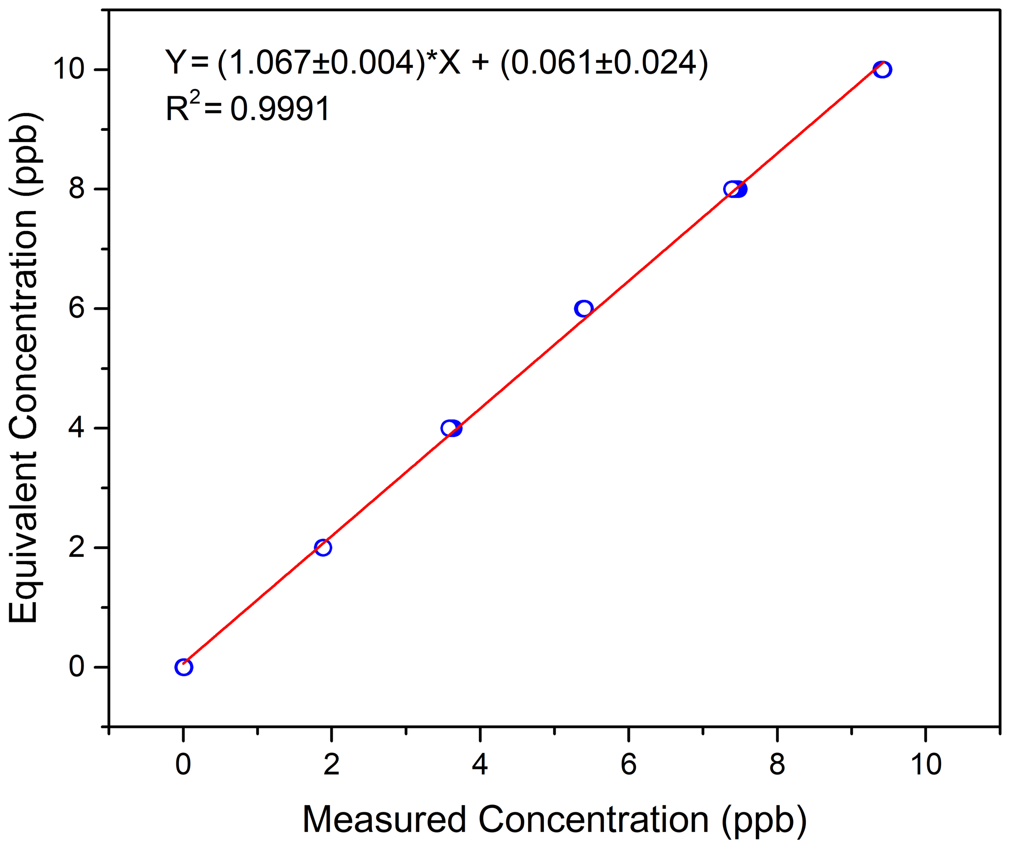
To verify the accuracy of the measurement results, isoprene gas with a known concentration was used to calibrate the instrument in the laboratory. The method is to close the emitting telescope and receiving telescope (close to zero optical path) in the laboratory, and then a series absorption cell is placed between the telescopes. Isoprene gas (10 ppm) was injected into the cells at a constant flow rate of 100 mL min⁻¹, and then the corresponding concentration under different cell combinations was measured, as shown in Fig. 3.

Figure 3 The scheme of the calibration system.

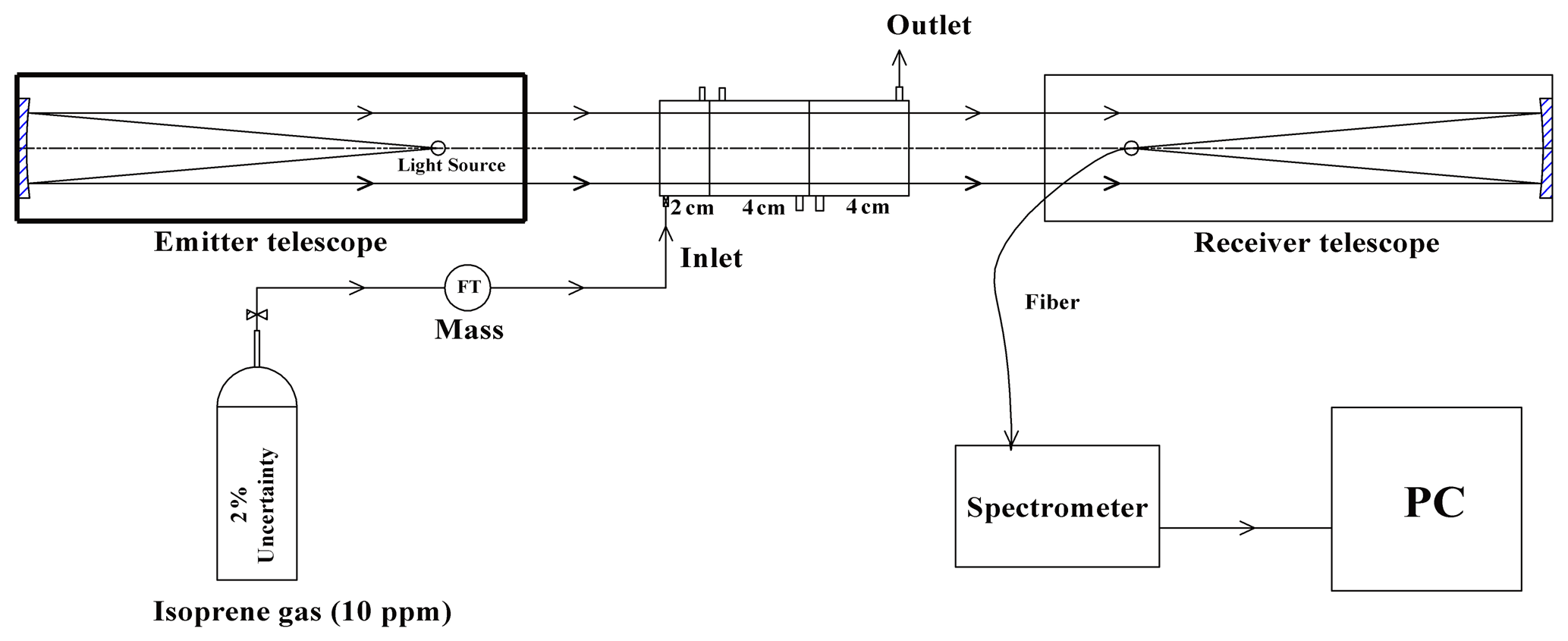
The absorption cell group is composed of one 2 cm and two 4 cm long cells in series. When using different combinations of cells, different equivalent concentrations (C_E) (equivalent to the average concentration in the 100 m optical path) can be obtained. The specific combination and corresponding equivalent concentrations, as well as the actual measurement concentrations (C_M), are shown in Table 2.

Table 2 The calibration results in different gas cell combinations.

Figure 4 shows the linear fit of the calibration results. The ordinate in the figure is the equivalent concentration, and the abscissa is the measured concentration. For six measuring points, including the zero point, the linear fitting correlation coefficient R is 0.9995. The relationship between the equivalent concentration and the measured concentration is shown in Eq. (1). For future measurement results of the actual atmosphere, Eq. (1) will be used to calibrate the measured data.

$$\begin{array}{}\text{(1)}& C_{\mathrm{E}}=(\mathrm{0.061}\pm \mathrm{0.024})+(\mathrm{1.067}\pm \mathrm{0.004})\times C_{\mathrm{M}}\end{array}$$

Figure 4 The linear fitting of calibration results for isoprene measurement.

3 Field comparison experiment and discussion

3.1 Comparison with online VOC results

To further verify the reliability of the DOAS method in actual atmospheric measurements, in July 2018, the field measurement results of the DOAS were compared with the online VOC (TH-300B online VOC monitoring system) analyzer (Zhu et al., 2020), which is based on the GC-MS technology. The DOAS instrument is installed on the seventh floor of the Environmental Science Building (31.344^∘ N, 121.518^∘ E) on Jiangwan Campus of Fudan University, as shown in Fig. 5. The optical path is about 25 m above the ground. The transmitting telescope is in the western part of the building (A in Fig. 5), while the receiving telescope is in the eastern part (B in Fig. 5). The distance between the telescopes is 75 m. The online VOC instrument is located at Xinjiangwan City monitoring station of the Shanghai Environmental Monitoring Center (C in Fig. 5). The straight-line distance is about 0.5 km to the south of the DOAS instrument. The coverage rate of plants around the observation sites was high, mainly including pine, camphor, etc., and a large number of lawns were also distributed. Meteorological parameters were recorded by an automatic weather station (CAMS620-HM, Huatron Technology Co. Ltd) co-located with the DOAS instrument.

Figure 5 Field measurement sites of DOAS and online VOCs, A is the transmitting telescope, B is the receiving telescope, and C is the online VOCs, and the yellow arrow is the light path of the DOAS. This map is sourced from © Baidu.

The comparison experiment was carried out from 1 to 23 July 2018. The temporal resolution of the DOAS was 1 min, while that of the online VOCs was 1 h. To match the temporal resolution, the DOAS data were averaged hourly. Moreover, the measured spectra with low light intensity and high integration time were excluded from the spectral fitting and data processing, which were mainly due to the unfavorable weather conditions influencing the measurements. The spectra were also corrected for offset before introducing fitting. Figure 6a shows the time series of the isoprene data measured by these two instruments, which are in good agreement. The average values of DOAS and online VOCs were 0.325 and 0.217 ppb, respectively, and the standard deviations (SDs) were 0.254 ppb (N=551) and 0.257 ppb (N=466), respectively. The average value of the DOAS results is higher than that of the online VOCs mainly because, at night, DOAS can still detect a certain concentration in most cases, most of which range between 0.02–0.10 ppb, while most of the online VOC data range between 0–0.05 ppb. Due to the missing online VOC data during the comparison period, in total 466 sets of hourly data were used to analyze the correlation between these two instruments. As shown in Fig. 6b, the correlation coefficient is 0.85, and the slope is 0.86.

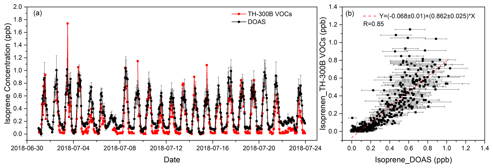
Figure 6 The comparison of hourly isoprene measured by DOAS and online VOCs during the field measurement.

The main reason for the difference in DOAS and online VOC results is that the sampling and measurement heights of the two instruments are different. The light path of the DOAS is about 25 m above the ground, while the sampling height of online VOC instrument is about 10 m. In addition to the 500 m distance between these two sites, the air sampled by the VOC analyzer or penetrated by the DOAS light beam is completely different. The inhomogeneous spatial distribution of isoprene will lead to different data results between the two instruments. Considering that the sampling of online VOCs occurs through the sampling tube, isoprene will be more or less lost during the sampling process, which could account for up to 10 % in some high-carbon VOCs (EPA, 2019). To ensure the authenticity and accuracy of the observed data, the working status and response of the TH-300B monitoring system were inspected every day. Daily calibrations were performed automatically at 00:00 to 01:00 LT. In addition, the external standard method for the FID (flame ionization detector) and the internal standard method for the MS were adopted. Implementing the daily calibration at midnight could move the online VOC-observed value close to the zero point, which may deviate from the actual abundance. Since the observation is in summer, there is also a very high temperature at night during the observation period, i.e., 27.1 ^∘C (19:00–06:00 LT next morning). In addition, the release of isoprene produced by the leaves of plants in the daytime is delayed to some extent, resulting in a certain concentration of isoprene remaining at night, so we think the DOAS data are more reasonable. These two reasons will eventually lead to DOAS measurement results higher than online VOC instruments, especially when the isoprene concentration is very low at night, and the difference is more obvious. On the other hand, the error of the DOAS method could also be a possible reason for the difference with the VOC analyzer.

It can also be seen in Fig. 6b that when the isoprene concentration is higher than 0.5 ppb, the measurement results of the two instruments show large scattering. The different measurement principles, especially the difference in sampling time, can also cause scattering of the results of the two instruments. Online VOCs only have about 50 % of the time (1 h) to be used for sampling, while the rest of the time is used for analysis. However, DOAS is an almost continuous measurement with just a small part of the time to be used for analysis (about 1 s min⁻¹); this difference will affect the consistency of the results. Meanwhile, there are various vegetation types between the instruments. When the wind direction changes, the emission of this part of vegetation will also cause a difference between the results of the instruments. However, in general, DOAS and online VOC analyzers show a good agreement in the comparison of the mean and correlation of measured data.

3.2 Detection limit evaluation

The detection limit of DOAS mainly depends on the signal-to-noise ratio of the spectrum. Under the condition of a zero light path in the laboratory, the zero noise (standard deviation of the results) of isoprene is 0.005 ppb, and the detection limit can be defined as 2 times the zero noise so that the detection limit of the system is 0.010 ppb (HJ 654-2013, 2013). However, in real atmospheric measurements, it is difficult to determine the actual detection limit due to the varied environment and the interference of other gases. The detection limit of DOAS in a real atmosphere is mainly determined by the residual of spectral fitting. This residual mainly comes from the absorption of interfering substances, the change in lamp spectral intensity and structure, the spectral shift caused by the change of ambient temperature of the spectrometer, and the noise of the detector. Since the stability of the light source and spectrometer will influence the fitting residual and instrumental performance, temperature control was adopted for the spectrometer and operating ambient environment. To reduce the influence of these factors on the measurement, during the spectral fitting process, the absorption of interfering substances and the spectral structure of the lamp must be considered together with the isoprene absorption spectrum. The lamp spectrum will also be introduced into the fitting process if an obvious lamp spectral structure was observed in the residual. At the same time, it is also necessary to calibrate the spectral drift. However, some residuals remain after spectral fitting due to possible imperfect reference spectra. Overall, the averaged measurement errors of isoprene were estimated to be lower than 20 %.

In the fitting band of isoprene, the absorption of NO, benzene and toluene are the main interference factors. The reason for the influence of NO is that there are three obvious absorption peaks of NO in the fitting band. After high-pass filtering, there is a component in the differential absorption cross section of NO similar to the variation frequency of isoprene's differential absorption spectrum. After an analysis of the measurement results, the impact of NO on isoprene is about 0.3 % of its concentration. However, the effect of NO mainly occurs in the morning and evening rush hours. The influence of benzene and toluene is mainly due to their strong absorptions in the fitting band of the spectrum. Their presence will lead to a significant reduction in the spectral intensity in this band, resulting in a reduction in the signal-to-noise ratio of the spectrum. During the comparison experiment, a high concentration of benzene or toluene occasionally occurs, resulting in a large fitting residual. Other aromatics, such as xylene and styrene, also absorb strongly in the fitting band, but because of their lower concentration in the natural atmosphere, their impacts on isoprene are significantly smaller than that of benzene and toluene. Although NH₃, SO₂ and NO₂ have absorption in the fitting band, their differential absorption variation frequency is significantly higher than that of isoprene and only overlaps in parts of fitting band so that they have little influence on the isoprene measurement. Figure 7a shows the absorption cross sections of benzene, toluene and isoprene, while Fig. 7b illustrates the differential absorption spectra (1 ppb km) of NO, SO₂, NO₂, NH₃ and isoprene obtained by applying high-pass filter, which is the same as the spectral fitting process. Moreover, the employment of the “clean” atmospheric spectrum, instead of the reference spectrum without any absorption under a zero optical path, also introduces the uncertainty into the spectral fitting because it may contain little isoprene absorption.

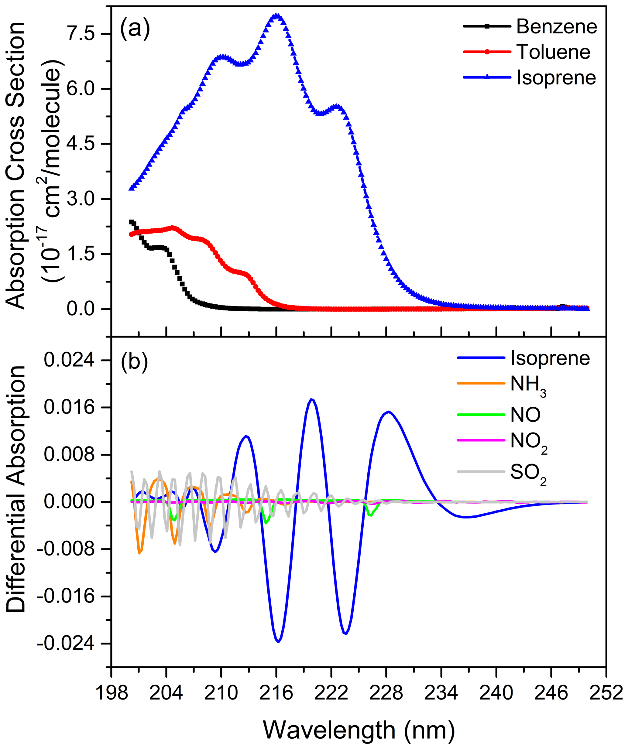
Figure 7 The absorption cross sections of benzene, toluene and isoprene (a), the differential absorption spectra (1 ppb km) of NO, SO₂, NO₂, NH₃ and isoprene (b).

Benzene, toluene, or NO, SO₂, NO₂ and NH₃ are present together with isoprene in the atmosphere. Therefore, their influences on isoprene measurement are common. To ensure the quality of the results, the data with a residual of more than 0.0005 are filtered out. In a total of 33 120 sets of data during 23 d of observation, 1137 sets were filtered out, and the valid rate of data was 96.6 %. The average residual of all valid data is 0.000234. To evaluate the detection limit of DOAS in a real atmospheric measurement, we calculated a statistic on 16 387 sets of data with the concentration of isoprene lower than 0.1 ppb (assuming that the isoprene in the atmosphere is close to zero at this time), and the standard deviation is 0.0499 ppb, so the detection limit of the DOAS instrument in the field measurement is no more than 0.1 ppb (twice the standard deviation).

4 Conclusion

This paper introduces, for the first time, the continuous online measurement of isoprene in the atmosphere by means of DOAS in the band of 202.71–227.72 nm. Although the current measurements of isoprene mainly consist of GC-MS, PTR-MS and CIMS methods, the DOAS method has the characteristics of high time resolution, rapid temporal response and simple operation. It is especially suitable for long-term online measurement in fields or forests where the travel is inconvenient, and the low cost of instrument is also conducive to building monitoring networks.

Under the condition of zero optical path in the laboratory, several equivalent concentrations were measured by using series absorption cells and known concentrations of isoprene gas. The correlation coefficient between the measured concentrations and the equivalent concentrations was 0.9996, and the slope was 1.065, indicating that the instrument has good linearity and accuracy. After 23 d of field comparisons, there was a good correlation between the results of the DOAS and online VOC instrument, with a correlation coefficient of 0.85 and a slope of 0.86. Considering the differences in measurement principles and the sampled air, the comparison results show good agreement between these two instruments.

To evaluate the detection limit of the DOAS instrument under actual atmospheric measurements, this study proposes to calculate the standard deviation of all the data when the measured concentration of isoprene in the ambient air is close to zero (< 0.1 ppb, n=16 387). It is estimated that the detection limit of DOAS is no more than 0.1 ppb under a measurement light path of 75 m. Therefore, DOAS is suitable for long-term monitoring in cities or areas with large vegetation coverage.