Determination of the emission rates of CO₂ point sources with airborne lidar

Anthropogenic point sources, such as coal-fired power plants, produce a major share of global CO₂ emissions. International climate agreements demand their independent monitoring. Due to the large number of point sources and their global spatial distribution, the implementation of a satellite-based observation system is convenient. Airborne active remote sensing measurements demonstrate that the deployment of lidar is promising in this respect. The integrated path differential absorption lidar CHARM-F is installed on board an aircraft in order to detect weighted column-integrated dry-air mixing ratios of CO₂ below the aircraft along its flight track. During the Carbon Dioxide and Methane Mission (CoMet) in spring 2018, airborne greenhouse gas measurements were performed, focusing on the major European sources of anthropogenic CO₂ emissions, i.e., large coal-fired power plants. The flights were designed to transect isolated exhaust plumes. From the resulting enhancement in the CO₂ mixing ratios, emission rates can be derived via the cross-sectional flux method. On average, our results roughly correspond to reported annual emission rates, with wind speed uncertainties being the major source of error. We observe significant variations between individual overflights, ranging up to a factor of 2. We hypothesize that these variations are mostly driven by turbulence. This is confirmed by a high-resolution large eddy simulation that enables us to give a qualitative assessment of the influence of plume inhomogeneity on the cross-sectional flux method. Our findings suggest avoiding periods of strong turbulence, e.g., midday and afternoon. More favorable measurement conditions prevail during nighttime and morning. Since lidars are intrinsically independent of sunlight, they have a significant advantage in this regard.

1 Introduction

CO₂ causes the strongest radiative forcing among all anthropogenic greenhouse gases (GHGs; e.g., Myhre et al., 2014). Therefore, it plays a crucial role with respect to human-induced climate change. In 2018, CO₂ reached a global annual average of 407.4 ppm at the Earth's surface, an increase of 47 % compared to the year ∼1750 (Friedlingstein et al., 2019). One third of all anthropogenic CO₂ emissions stem from localized point sources, in particular coal-fired power plants (Oda and Maksyutov, 2011). For Europe, they even account for 45 % of CO₂ emissions (Super et al., 2020). The Paris Climate Agreement aims to reduce anthropogenic GHG emissions by means of nationally determined contributions (NDCs) which are based on national capabilities and the level of economic development (UNFCCC, 2015). Therein it is foreseen that as of 2023 a global stocktake will take place every 5 years. This requires independent measurements to verify each nation's emission reports of CO₂ but also of other greenhouse gases, such as CH₄. Currently, there is no independent global emission verification system available, and a complete record of all emissions globally is still far from reality. To achieve this goal, satellite missions are indispensable. Satellite missions are expected to detect CO₂ emissions from large power plants and cities, e.g., the future European carbon constellation CO2M (Bézy et al., 2019; Broquet et al., 2018; Kuhlmann et al., 2020) and other mission ideas still in the pre-development phase (Kiemle et al., 2017; Strandgren et al., 2020). Furthermore, CH₄ emissions can also be detected, as is done by GHGSat-D for coal mine ventilation shafts (Varon et al., 2020) or the Sentinel-5 Precursor for the oil- and natural-gas-producing sector (Pandey et al., 2019; Zhang et al., 2020). Under particularly favorable conditions, it is already possible to detect CO₂ emissions of power plants from space, as is done with data from NASA's OCO-2 mission (Nassar et al., 2017; Reuter et al., 2019). However, at the moment no operating satellite mission is able to quantify emissions from large power plants on a regular basis. In the development phase for potential missions, airborne measurement campaigns serve as a test of the methods. During the operating phase, they are needed for verification of the space-borne results.

In May/June 2018, the CoMet (Carbon Dioxide and Methane Mission) field campaign took place. The objective of CoMet was to investigate the fluxes of the major human-influenced GHGs on local, regional, and sub-continental scales. These fluxes were to be determined more precisely than previously possible. Furthermore, supporting activities for GHG stocktaking were provided. The CoMet campaign saw the deployment of a suite of airborne instruments to measure atmospheric CH₄ and CO₂, alongside a variety of ground-based instruments. In particular, the synergetic use of active remote sensing (lidar) (Amediek et al., 2017; Wildmann et al., 2020), passive spectrometry (Krautwurst et al., 2021; Luther et al., 2019), and in situ measurements (Fiehn et al., 2020; Gałkowski et al., 2021; Kostinek et al., 2020) supported by modeling activities (Chen et al., 2020; Nickl et al., 2020), as well as the validation of existing (e.g., Sentinel-5P, GOSAT, Greenhouse gases Observing SATellite) and the preparation of upcoming (e.g., MERLIN, MEthane Remote sensing Lidar missioN) GHG satellite missions, was aimed at.

Hereby, the German research aircraft HALO (High Altitude and Long Range Research Aircraft) acted as the airborne flagship of that campaign. HALO was equipped with the new airborne CO₂ and CH₄ IPDA (integrated path differential absorption) lidar CHARM-F (CO₂ and CH₄ Atmospheric Remote Monitoring Flugzeug) built and operated by DLR as an airborne demonstrator of the upcoming MERLIN mission (Ehret et al., 2017). CHARM-F simultaneously measures the column-averaged dry-air mixing ratios of carbon dioxide (XCO₂) and methane (XCH₄) between the aircraft and ground (Amediek et al., 2017). The influence of other trace gases, in particular H₂O, on the mixing ratio measurements is negligible. As a result of the pulse repetition frequency (50 Hz, double pulse) and divergence (∼1.5 mrad), the pattern on the ground is a sequence of overlapping footprints. The vertical column measurements are insensitive to the vertical redistribution of the trace gases. The insensitivity towards optically thin clouds, aerosol layers, and varying surface albedo, and the instrument design with, e.g., active laser frequency control, is a further strong asset of the IPDA lidar approach. Albedo variations basically affect the measurement precision (statistical uncertainty), whereas the influence on the bias is negligible (Amediek et al., 2009).

During the CoMet campaign, HALO probed various local plumes of different coal-fired power plants. As a case study, the paper in hand focuses on the measurement flight of 23 May 2018, in which the CO₂ exhaust plume of the power plant Jänschwalde, close to the Polish–German border, was surveyed. The specific goal is to quantify the CO₂ fluxes of the power plant. An established method for quantifying emission rates of point sources is the cross-sectional flux method, which is a product of mean wind speed and an integrated concentration enhancement along a cross-sectional overflight of the exhaust plume. This principle has been applied to air- and space-borne nadir-viewing remote sensing (Krings et al., 2018; Menzies et al., 2014; Varon et al., 2018; Reuter et al., 2019), mobile ground-based sun-viewing remote sensing (Luther et al., 2019), and airborne in situ measurements (Cambaliza et al., 2014; Conley et al., 2016; Fiehn et al., 2020; White et al., 1976). Amediek et al. (2017) have described how this principle can be realized with CHARM-F. Using CHARM-F data from the respective overflights, we strive to accurately assess the error and advance the general methodology.

When determining the cross-sectional flux, one of the major error sources is the local wind field: on the one hand, because the wind speed is directly included in the calculation, on the other hand, because atmospheric turbulence can broaden or constrict the spatial extent of the exhaust plume. This is a well-known problem which contributes significantly to the measurement error (Kuhlmann et al., 2019; Luther et al., 2019; Strandgren et al., 2020; Varon et al., 2018; Jongaramrungruang et al., 2019; Kumar et al., 2020). Consequently, the observed CO₂ column enhancements between subsequent plume transects may vary considerably despite a constant emission rate. We hypothesize that these turbulence-induced variations dominate the measurement error of the emission estimates rather than the GHG column measurement uncertainty itself. To assess the impact of this atmospheric turbulence on our measurement results, we perform a large eddy simulation (LES) in order to resolve local plume structures. By doing so, we can compare different ambient weather and turbulence conditions. We aim to separate more and less favorable conditions, to determine an adequate distance between emission source and measurement locations, and to find out how many independent plume measurements will be necessary in order to obtain an appropriate emission rate accuracy as a function of those environmental conditions.

This paper is organized as follows. Section 2 introduces the IPDA lidar method and describes the retrieval of the emission rate and the methodical errors. Section 3 reports on the plume measurement results. Section 4 provides the simulation setup, while the subsequent results are presented in Sect. 5. A discussion is given in Sect. 6, followed by the conclusion in Sect. 7 and the outlook in Sect. 8.

2 Cross-sectional flux method

2.1 Flux calculation

The dataset underlying this work originates from the IPDA lidar CHARM-F. A more detailed description of the lidar system can be found in Amediek et al. (2017). At its core, CHARM-F consists of a pulsed, tunable laser source and a detector. Installed on an aircraft or satellite, the nadir-oriented lidar emits two laser pulses that propagate through the atmosphere until they are backscattered at a surface. The two backscattered laser pulses are detected by the lidar. The wavelength of one laser pulse corresponds to the absorption wavelength of the greenhouse gas under consideration. In the following, this laser pulse is referred to as online. Due to molecular absorption, the intensity of the online laser pulse decreases while propagating through the atmosphere. The wavelength of the other (offline) laser pulse is slightly shifted such that almost no absorption by the greenhouse gas takes place, but the interaction with the remaining atmospheric components is unaltered.

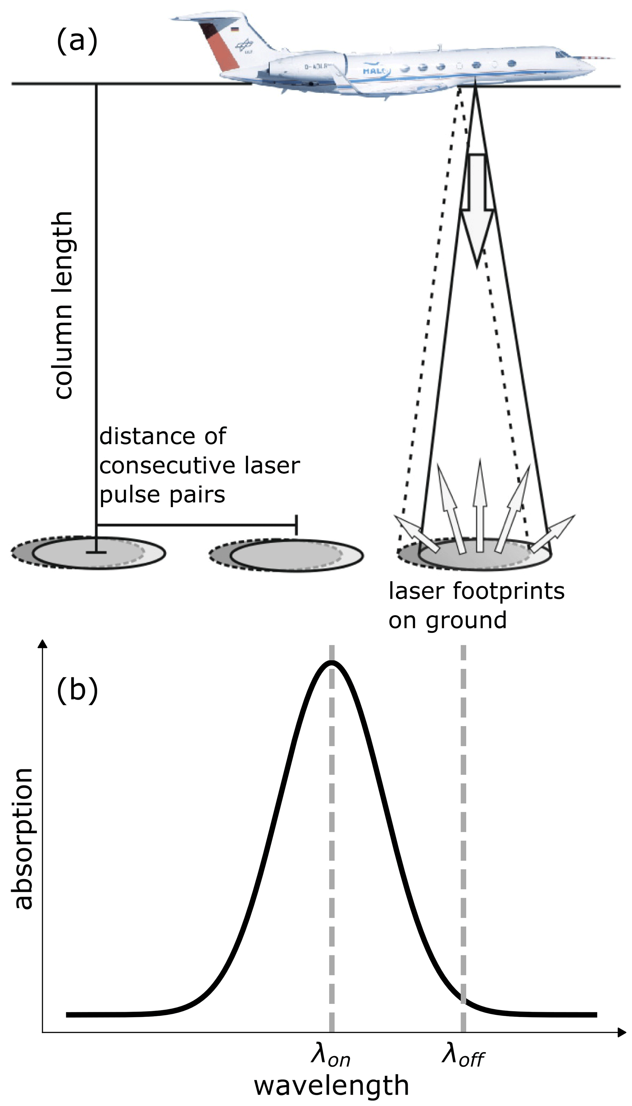
Figure 1 Figure by Amediek et al. (2017). The measurement geometry of a lidar, illustrated by the example of CHARM-F carried on the aircraft HALO. Two laser pulses are emitted towards the earth with a delay of 500 µs. The laser pulse with the wavelength λ_on is on the absorption line of CO₂ (1572.02 nm), and the laser pulse with the wavelength λ_off is not (1572.12 nm). By comparing the backscattered intensities, the CO₂ concentration in the measured cone volume can be calculated. The measured volume is usually referred to as a vertical air column since the column length, i.e., the aircraft's altitude above ground (∼6500 m), is very large compared to the diameter of the reflecting surfaces (∼10 m). The distance of consecutive laser pulse pairs is 3 m. The black line in (b) schematically depicts the measurement principle, not the actual spectral absorption line shape of CO₂.

Using a beam splitter, a small part of both the online and the offline laser pulse energy (E_on/off) is deflected onto a detector while still in the lidar system. Together with the radiation fluxes entering the lidar telescope P_on/off, the differential optical absorption depth (DAOD) can be calculated (Ehret et al., 2008).

$$\begin{array}{}\text{(1)}& \text{DAOD}={\displaystyle \frac{\mathrm{1}}{\mathrm{2}}}\cdot \ln \left({\displaystyle \frac{P_{\text{off}}/E_{\text{off}}}{P_{\text{on}}/E_{\text{on}}}}\right)\end{array}$$

Note that for the DAOD a single value is obtained for the entire vertical air column. It is a metric for the greenhouse gas concentration of the measured column and is also defined by the following relationship.

$$\begin{array}{ll}\text{(2)}& {\displaystyle }\text{DAOD}& {\displaystyle }={\text{DAOD}}_{\mathrm{b}}+\mathrm{\Delta }\text{DAOD}{\displaystyle }& {\displaystyle }={\text{DAOD}}_{\mathrm{b}}+{\displaystyle \frac{\mathrm{1}}{M}}\underset{\mathrm{0}}{\overset{\text{fl}}{\int }}\mathrm{\Delta }\mathit{\sigma }\left(z\right)\cdot \mathrm{\Delta }c\left(z\right)\mathrm{d}z\\ {\displaystyle }& {\displaystyle }\approx {\text{DAOD}}_{\mathrm{b}}+{\displaystyle \frac{\stackrel{\mathrm{‾}}{\mathrm{\Delta }\mathit{\sigma }}}{M}}\underset{\mathrm{0}}{\overset{\text{fl}}{\int }}\mathrm{\Delta }c\left(z\right)\mathrm{d}z\end{array}$$

Here, DAOD_b is the background differential absorption optical depth, ΔDAOD is the enhancement in the DAOD induced by the plume, M is the molecular mass of CO₂ in grams (g), Δc(z) is the enhanced CO₂ density induced by the plume in grams per cubic centimeter (g cm⁻³), and Δσ(z) is the difference between the CO₂ absorption cross section for the two laser wavelengths given in square meters (m²; cf. Fig. 1). It is referred to as the differential absorption cross section. Generally, Δσ(z) is not constant over the plume's vertical extension due to the decreasing pressure with altitude. However, the decreases in pressure associated with typical vertical plume extensions are small. As an approximation, we use the mean value over the vertical extent of the plume. This aspect is discussed in more detail in Sect. 3. The vertical integral limits are the ground (z=0 m) and the respective height of the aircraft flights (z = fl). Variations in flight altitude, as well as topography, may cause variations in the surveyed column length and thus ultimately in the measured DAOD. In this study, these variations are negligible since the flight altitude was deliberately kept constant, and the topography around the power plant under consideration is sufficiently flat.

This DAOD dataset is used to determine the CO₂ emission rate of a point source utilizing the flux calculation method introduced by Amediek et al. (2017). As schematically depicted in Fig. 2, a crossing of the exhaust plume leads to a DAOD enhancement. This is caused by the additional absorption of laser radiation by the CO₂ molecules of the plume. The instantaneous flux through the lidar cross-section, at the moment of the overflight, is given in kilograms per second (kg s⁻¹) and denoted by q.

$$\begin{array}{}\text{(3)}& q=A\cdot {\displaystyle \frac{M}{\stackrel{\mathrm{‾}}{\mathrm{\Delta }\mathit{\sigma }}}}\cdot u\cdot \sin \left(\mathit{\phi }\right)\end{array}$$

Given in meters (m), the parameter A corresponds to the integrated DAOD enhancement over the background DAOD in the direction of the aircraft flight track as shown in Fig. 2b. In the following, it is referred to as integrated enhancement. The mean horizontal wind speed u is given in meters per second (m s⁻¹), and the angle between the wind direction and the aircraft's flight direction is denoted as φ (in the following referred to as relative wind direction). Furthermore, it is assumed that no uptake by the soil takes place when the gas plume hits the ground and that the flight altitude is high enough (i.e., well above the planetary boundary layer, PBL) to cover the entire vertical extent of the plume.

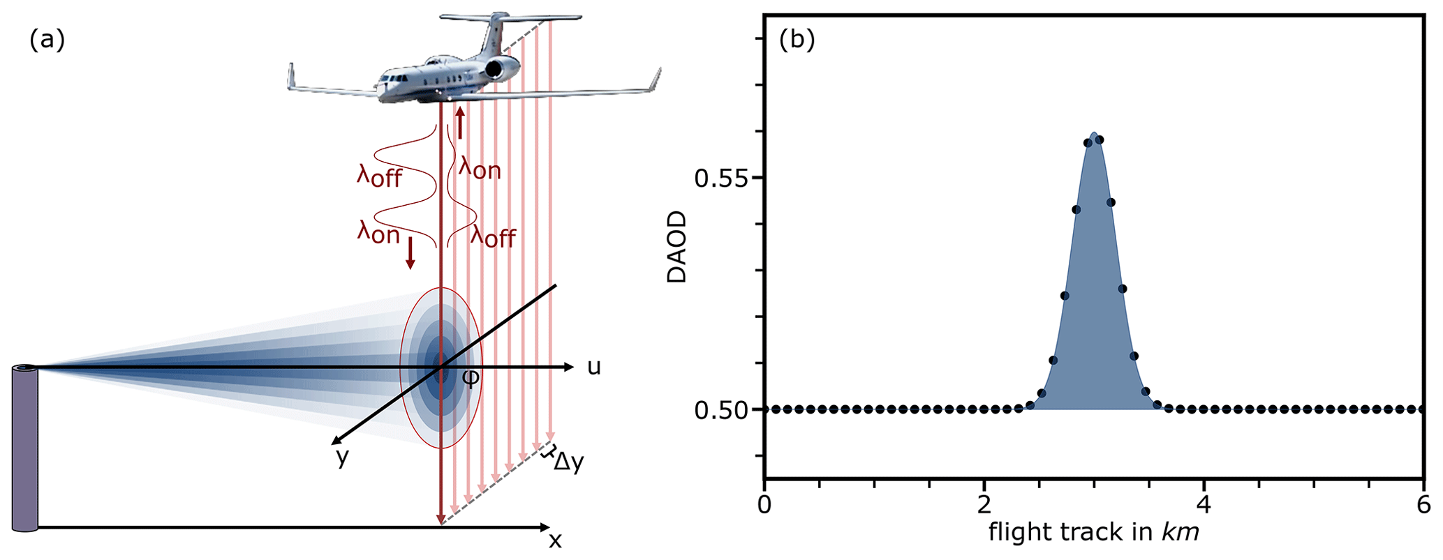
Figure 2 Crossing an exhaust plume illustrated by the example of CHARM-F carried on the aircraft HALO. (a) Two laser pulses are emitted towards the earth with a short delay. The laser pulse with the wavelength λ_on is on the absorption wavelength of CO₂, and the laser pulse with the wavelength λ_off is not. By comparing the backscattered intensities, the DAOD can be calculated (see Sect. 2.1). An ideal exhaust plume of a point source has a Gaussian-shaped mean concentration distribution both horizontally and vertically. (b) A perpendicular crossing of the plume yields a Gaussian-shaped DAOD dataset.

The two closely spaced sounding wavelengths are selected in such a way that the impact from unknown particles is minimized while keeping the absorption by water vapor as low as possible. This is due to the very weak water vapor differential absorption cross section, which is more than 4 orders of magnitude smaller than the differential absorption cross section for CO₂. Thus, the influence of additional water vapor in the plume released by the cooling or coal drying systems of the power plant is negligible (Kiemle et al., 2017). Moreover, the selected CO₂ absorption line is sufficiently temperature-insensitive such that the influence of temperature variations within the plume can be neglected (see also Kiemle et al., 2017). Under these conditions, the flux error is mainly driven by uncertainties in the four parameters A, $\stackrel{\mathrm{‾}}{\mathrm{\Delta }\mathit{\sigma }}$, u, and φ. Assuming that these parameters are not correlated, the relative accuracy in the flux calculation can then be estimated by error propagation means.

$$\begin{array}{}\text{(4)}& {\displaystyle \frac{\mathit{\delta }q}{q}}=\sqrt{{\left({\displaystyle \frac{\mathit{\delta }A}{A}}\right)}^{\mathrm{2}}+{\left({\displaystyle \frac{\mathit{\delta }\left(\stackrel{\mathrm{‾}}{\mathrm{\Delta }\mathit{\sigma }}\right)}{\stackrel{\mathrm{‾}}{\mathrm{\Delta }\mathit{\sigma }}}}\right)}^{\mathrm{2}}+{\left({\displaystyle \frac{\mathit{\delta }u}{u}}\right)}^{\mathrm{2}}+{\left({\displaystyle \frac{\mathit{\delta }\mathit{\phi }}{\tan \left(\mathit{\phi }\right)}}\right)}^{\mathrm{2}}}\end{array}$$

The relative uncertainties in these parameters are denoted by $\mathit{\delta }A/A$, $\mathit{\delta }\left(\stackrel{\mathrm{‾}}{\mathrm{\Delta }\mathit{\sigma }}\right)/\stackrel{\mathrm{‾}}{\mathit{\delta }\mathit{\sigma }}$, and $\mathit{\delta }u/u$ denote the relative uncertainties in these parameters. From this, it is obvious that crossing the plume perpendicular to the wind direction as displayed in Fig. 2a would give the highest accuracy for any fluctuation in the wind direction δφ. On the other hand, atmospheric conditions at low wind speeds or situations with high atmospheric turbulence are in general less favorable because of the high uncertainty in the mean wind speed and wind direction. Varon et al. (2018) have identified 2 m s⁻¹ as the minimum threshold of wind speed for the applicability of the cross-sectional flux method. This minimum value is also referred to by Sharan et al. (1996), arguing that above this threshold, advection dominates over diffusion.

2.2 Background separation

For the calculation of the integrated enhancement A and its uncertainty, it is crucial to distinguish between the DAOD value attributable to the background concentration of CO₂ and the fraction attributable to the exhaust plume of the point source. As shown in Eq. (2), the measured DAOD along the flight track is the sum of background term DAOD_b and the enhancement due to the plume interaction (ΔDAOD). A complicating factor is that the background term may not be constant. There are small variations in local CO₂ concentration from other anthropogenic sources (traffic, cities, etc.) or local interaction with the biosphere. Also, small CO₂ gradients caused by the sounding of different air masses in the vicinity of the plume may have an impact on the background term. In the following, we describe a suitable method that enables us to extract ΔDAOD from the measured dataset while allowing the background term to be variable.

An example of the plume extraction procedure is shown in Fig. 3. The plume must first be detected as an enhancement not attributable to noise in the data. For this, we examine a 0.2 km running mean of the DAOD dataset (Fig. 3a). The choice of 0.2 km is made because it corresponds to the diameter of the pixels of the simulation (see Sect. 4). The larger the window for the running mean is, the less noise is present and the clearer the plume enhancement can be seen. Then again, peaks threaten to be blurred if the window width becomes too large.

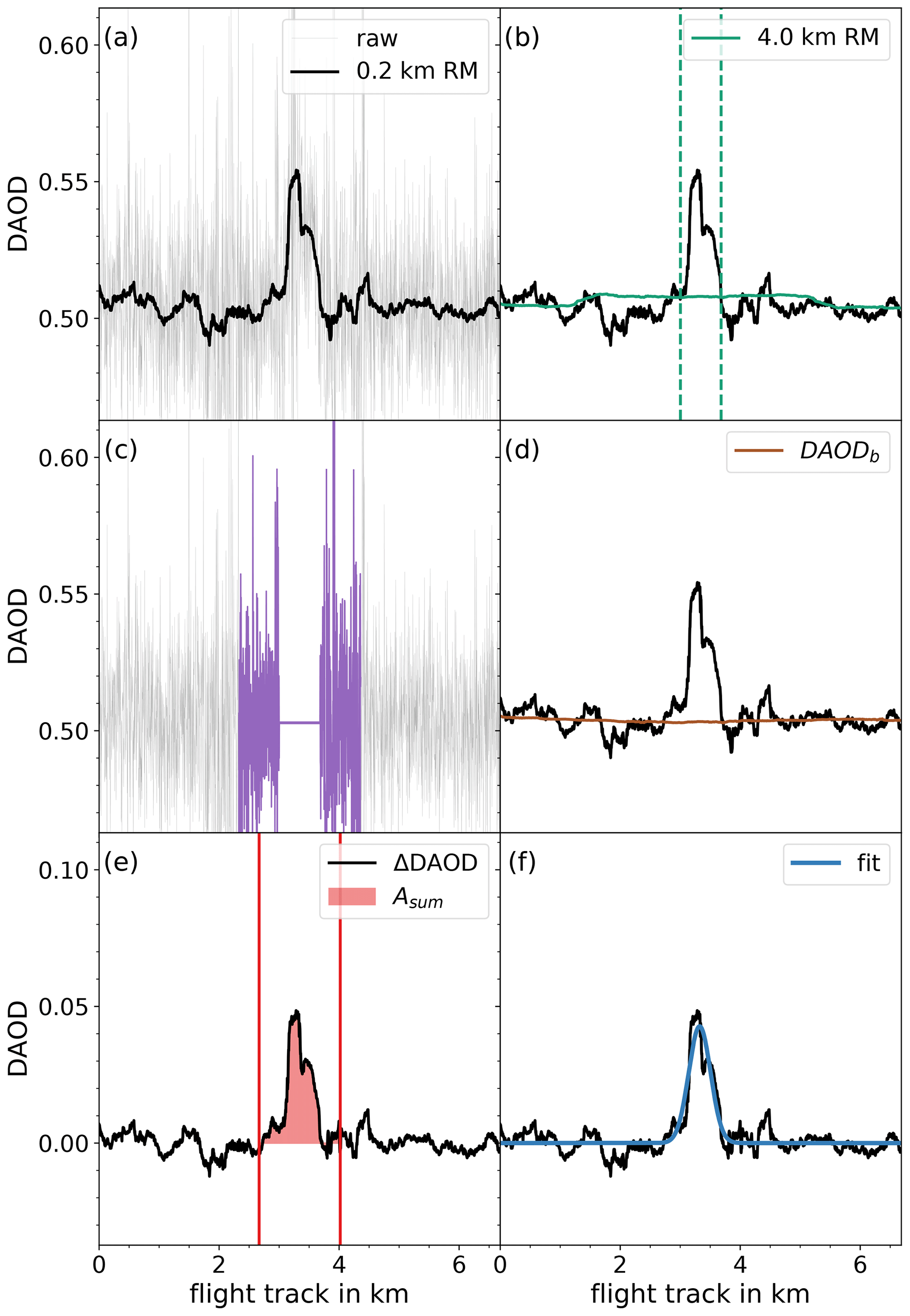
Figure 3 Plume crossing at a point source distance of 1.53 km. In (a) the gray curve shows the raw data, with a standard deviation of 5.2 %, while the black curve shows a 0.2 km (64 data points) running mean (RM), with a standard deviation reduced to 0.9 %. In (b) the green curve is a 4 km (1293 data points) RM. Vertical dashed green lines mark the intersections between the 0.2 and 4 km RMs, which are defined as the plume's limits. The color purple in (c) shows the region of the data used to construct a mean value of the data before and after the plume's limits. This mean value is used to bypass the plume enhancement and is also colored purple. In (d) again a 4 km running mean over the bypassed dataset is shown in brown. These data, which have slight variability, are used as the background term DAOD_b. Finally, in (e) and (f) the enhanced term ΔDAOD, i.e., difference between 0.2 km RM and DAOD_b, is plotted in black. Note the different scale on the y axis. In (e) the area underneath the curve is colored red as an example of the parameter A_sum determined with a Riemann sum. Alternatively, a Gaussian fit can be applied to ΔDAOD, providing the parameter A_fit as a fit-parameter, shown as a blue line in (f).

Starting from the middle of the plume enhancement, we define the plume's limits as the intersections between the 0.2 km running mean (RM) and another 4 km running mean (Fig. 3b). Applying a running mean broadens and flattens the plume. For larger running mean widths, such as 4 km, the flattening is so severe that the plume is only distinguishable from the background as a raised plateau (see Fig. 3b). The limits are then defined as the intersections between the 0.2 and the 4 km running means. For the calculation of this mean we consider a window with a width equal to that of the plume, colored violet in Fig. 3c. At last, we execute another 4 km running mean over the raw dataset with bypassed plumes, resulting in the background term DAOD_b, shown in brown in Fig. 3d. This procedure allows for a variability in the background term on a scale of a few hundred meters. Smaller scale gradients cannot be attributed to the background and are incorporated in the enhancement term ΔDAOD, thereby not being distinguishable from noise.

The mean wind speed u and its mean relative direction φ are extracted from model data provided by ECMWF. The molecular mass M and the differential absorption cross section Δσ are physical properties of CO₂ and available in various databases such as HITRAN2016 (Gordon et al., 2017). The only parameter that results from a measurement by CHARM-F, or a respective simulation, is the integrated enhancement A. For this purpose Amediek et al. (2017) described two distinct methods. The first method is a Riemann sum over all enhancement values ΔDAOD_i multiplied by their respective spatial distance Δy_i between two successive data points.

$$\begin{array}{}\text{(5)}& A_{\text{sum}}=\left(\sum _i\mathrm{\Delta }{\text{DAOD}}_i\cdot \mathrm{\Delta }{y}_i\right)\end{array}$$

The second method makes use of the fact that, on average, the plume is subject to Gaussian dispersion behavior. According to the function F(y) in Eq. (6), a nonlinear least squares fit is applied to the ΔDAOD values of the plume.

$$\begin{array}{}\text{(6)}& F\left(y\right)={\displaystyle \frac{A_{\text{fit}}}{A_{\mathrm{2}}\cdot \sqrt{\mathrm{2}\mathit{\pi }}}}\cdot e^{-\frac{\mathrm{1}}{\mathrm{2}}\cdot {\left(\frac{y-A_{\mathrm{1}}}{A_{\mathrm{2}}}\right)}^{\mathrm{2}}}\end{array}$$

By doing so the integrated enhancement is obtained as the fit parameter A_fit. A₁ is the peak's position along the flight track and A₂ the turbulent dispersion parameter, which is a measure for the width of the plume. The fit method yields very low values for the uncertainty of the parameter A. However, the Riemann sum is not depending on any model assumption for the calculation of the integrated ΔDAOD along the flight track. Both methods were investigated in the course of this work and showed nearly identical results. Therefore, the results in Table 1 correspond to the mean value of the two methods.

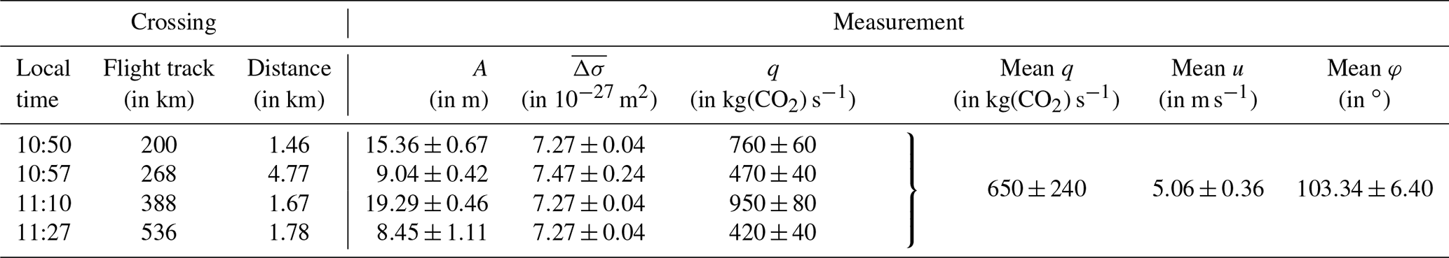
Table 1 Flight measurement results of individual crossings for the Jänschwalde power plant on 23 May 2018, following the nomenclature of Eq. (3).

3 Airborne measurements

In this work the measurement flight of HALO on 23 May 2018 between 10:24 and 11:36 CEST (Central European summer time) is investigated. Located in the southeast of the German federal state of Brandenburg close to the Polish–German border, the Lausitz Energie Kraftwerke AG (LEAG) operates the coal-fired power plant Jänschwalde. It is one of the largest power plants in Europe both in terms of annual electricity generation and annual CO₂ emissions. For the year 2017, the power plant operators have reported an emission quantity of 24.0 Tg (CO₂) to the European Environment Agency (E-PRTR, 2020). The exhaust gases of this power plant are emitted through the cooling towers at a height of ∼120 m. Figure 4 shows the flight track of the aircraft, along with a picture of the cooling towers. In total, the point source was flown over seven times downwind, two times upwind, and once directly over the cooling towers. In three of the downwind overflights, no enhancement in DAOD is visible. For these transects, the distance to the point source is greater than 4.6 km. At such distances, it can be assumed that the exhaust gases are too diluted with the surrounding air to generate a measurable signal.

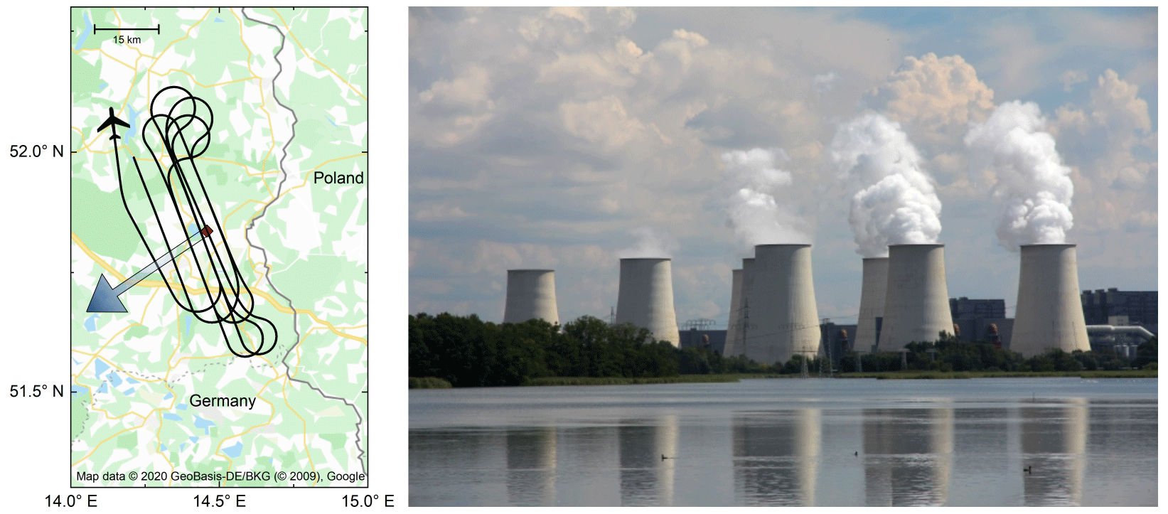
Figure 4 Flight track of HALO in the vicinity of the coal-fired power plant Jänschwalde. The black line on the left depicts the flight track of HALO between 10:24 and 11:36 on 23 May 2018. The red square marks the position of the power plant Jänschwalde. The arrow shows the mean wind direction during the observation period. The right picture shows the nine cooling towers facing southwest. There the exhaust is released. The towers have a height of 120 m and distances of 250 and 50 m between each other.

In order to evaluate the uncertainty of the calculated integrated enhancement, a total of 15 different data subsets centered on the plume's position, with varying width, are examined. To ensure that the Riemann sum completely covers the plume, the smallest subset is twice as wide as the plume limits, determined according to Fig. 3. The width of the remaining subsets is expanded by 400 m each.

To further evaluate Eq. (3), the differential absorption cross section Δσ is calculated using the Voigt-profile model with input from the HITRAN 2016 database for the line parameters (Gordon et al., 2017). This calculation requires the knowledge of pressure and temperature profiles, which are extracted from the simulation introduced in Sect. 4. For the lidar measurements, the online wavelength was tuned to the CO₂ absorption line center at λ_on=1572.02 nm, while the offline wavelength was adjusted to λ_off=1572.12 nm in the wing of this line (cf. Fig. 1b). Based on this wavelength selection and a flight altitude of 8000 m, the background DAOD_b is approximately 0.5, while the plume causes a ∼10 % enhancement to this value (∼0.05), as depicted in Fig. 3. The absorption cross section is not constant over the plume's vertical extension mainly due to the decreasing pressure and resulting decrease in collisional line broadening with altitude. The relative change in the absorption cross section along the vertical course of the plume depends on the exact online position with respect to the absorption line center. To take a possible cross-section change for our measurements into account, representative mean values for the distances at x₁≈1500 and x₂≈4700 m (see Table 1) are calculated using the slender plume approximation (Amediek et al., 2017; Seinfeld and Pandis, 1997).

7$$

In this equation, the ground (z=0 m) and the maximum (z=4000 m) denote the integration boundaries, and h is the height of the cooling towers. The key parameter in this equation is the turbulence parameter σ_z, which is a proxy for the plume extension in the vertical direction, at the respective distance. Different expressions for this parameter for various atmospheric stability conditions can be found in the literature, e.g., Seinfeld and Pandis (1997).

Assuming a moderately turbulent atmosphere, we found plume widths of σ_z=170 and 600 m for the two distances. However, if the atmospheric turbulence is less pronounced, the vertical plume widths are only σ_z=90 and 250 m. Due to the lack of further information on turbulence characteristics during our measurements, we consider both plume widths in the calculation below. The change in Δσ(z) versus altitude above ground in Eq. (8) is calculated at grid cell spacing of 1 m in the vertical direction using the following second order polynomial function.

$$\begin{array}{ll}\text{(8)}& {\displaystyle }\mathrm{\Delta }\mathit{\sigma }\left(z\right)=& {\displaystyle }\mathrm{7.10652}\times {\mathrm{10}}^{-\mathrm{27}}{\mathrm{m}}^{\mathrm{2}}{\displaystyle }& {\displaystyle }+\mathrm{8.60755}\times {\mathrm{10}}^{-\mathrm{31}}\mathrm{m}\cdot z\\ {\displaystyle }& {\displaystyle }+\mathrm{8.02673}\times {\mathrm{10}}^{-\mathrm{35}}\cdot z^{\mathrm{2}}\end{array}$$

Consequently, the differential absorption cross section at the height of the ground (70 m a.s.l.) corresponds to $\mathrm{\Delta }\mathit{\sigma }(z=\mathrm{0}\mathrm{m})=\mathrm{7.10652}\times {\mathrm{10}}^{-\mathrm{27}}$ m². The constant factors of this equation are the result of fitting this function to some representative cross-section values from Voigt-profile calculations over the altitude range of 4000 m. The deviations of this approximation to the exact Voigt-profile calculations are less than 0.1 %, which is regarded as negligible. Finally, Eq. (7) gives the following results:

$$\stackrel{\mathrm{‾}}{\mathrm{\Delta }\mathit{\sigma }\left(x_{\mathrm{1}}=\mathrm{1500}\mathrm{m}\right)}=\mathrm{7.27}\times {\mathrm{10}}^{-\mathrm{27}}{\mathrm{m}}^{\mathrm{2}}\pm \mathrm{0.04}\times {\mathrm{10}}^{-\mathrm{27}}{\mathrm{m}}^{\mathrm{2}}$$

and

$$\stackrel{\mathrm{‾}}{\mathrm{\Delta }\mathit{\sigma }\left(x_{\mathrm{2}}=\mathrm{4700}\mathrm{m}\right)}=\mathrm{7.47}\times {\mathrm{10}}^{-\mathrm{27}}{\mathrm{m}}^{\mathrm{2}}\pm \mathrm{0.24}\times {\mathrm{10}}^{-\mathrm{27}}{\mathrm{m}}^{\mathrm{2}}.$$

The overscore indicates the mean value of the aforementioned turbulence scenarios with corresponding plume vertical widths at each distance, and the errors indicate the differences. Close to the source (∼1500 m), the relative cross-section uncertainty is ∼0.6 % and therefore negligible, whereas, at a distance of 4700 m, the relative error is ∼3.2 % and not negligible in the overall error budget outlined by Eq. (4).

Possible systematic errors due to uncertainties in the line parameters are less than 2 % (Gordon et al., 2017). Errors resulting from the wavelength setting with the CHARM-F instrument are considered very small compared to the other contributors and therefore need not to be extensively discussed in this study (∼0.5 %; see Amediek et al., 2017).

The wind data are taken from operational analysis data of the ECMWF model. This is done by first interpolating the 4D gridded model data onto the flight path at the altitude of the power plant's exhaust shaft. Secondly, a mean value of the wind speed and direction along the flight track, together with an estimate of their relative errors, are calculated according to Ackermann (1983).

Table 1 shows the measured integrated enhancements, the wind data, and the resulting fluxes for the four exploitable overflights, alongside the obtained mean values, under the assumption that during the measurement both the wind direction and the wind speed were reasonably constant. The flight segments were not exactly perpendicular to the mean wind direction. With a relative angle of φ=103^∘ a correction factor of $\sin \left(\mathrm{103}{}^{\circ }\right)=\mathrm{0.97}$ is applied (see Eq. 3). The mean wind speed is well above the threshold of 2 m s⁻¹, introduced at the end of Sect. 2.1.

The individual flux uncertainties, calculated with Eq. (4), are relatively small and range between 8 %–10 %. It is to be emphasized that the integrated enhancement A is the only parameter in the calculation of the instantaneous flux in Eq. (3) coming from the IPDA lidar measurement itself. On average, $\mathrm{2}/\mathrm{10}$ of this individual measurement uncertainty is due to the uncertainty of the integrated enhancement $\mathit{\delta }A/A$. Taken together, $\mathrm{1}/\mathrm{10}$ can be attributed to the uncertainty of the mean differential absorption cross section of CO₂ $\mathit{\delta }\left(\stackrel{\mathrm{‾}}{\mathrm{\Delta }\mathit{\sigma }}\right)/\stackrel{\mathrm{‾}}{\mathit{\delta }\mathit{\sigma }}$ and the mean relative wind direction $\mathit{\delta }\mathit{\phi }/\tan \left(\mathit{\phi }\right)$. The major contributor to the flux uncertainty, however, is the uncertainty of the mean wind speed $\mathit{\delta }u/u$, which accounts for $\mathrm{7}/\mathrm{10}$.

The reported value of 760 kg(CO₂) s⁻¹ (24.0 Tg(CO₂) yr⁻¹) (E-PRTR, 2020) lies within the error range of the mean value of 650±240 kg(CO₂) s⁻¹ (20.3±7.9 Tg(CO₂) yr⁻¹). Nevertheless, the variations between the individual crossings are very large, both in the integrated enhancement A and in the calculated fluxes. The second and third crossings differ by approximately a factor of 2 (see Table 1). These variations cannot be explained by our uncertainty estimation but rather by atmospheric turbulence that distorts the plume. Therefore, this work further investigates the influence of atmospheric turbulence and the resulting inhomogeneity in the propagation of exhaust plumes. To achieve this, we make use of the mesoscale numerical weather prediction system model WRF (Weather Research and Forecasting model).

4 Simulation setup

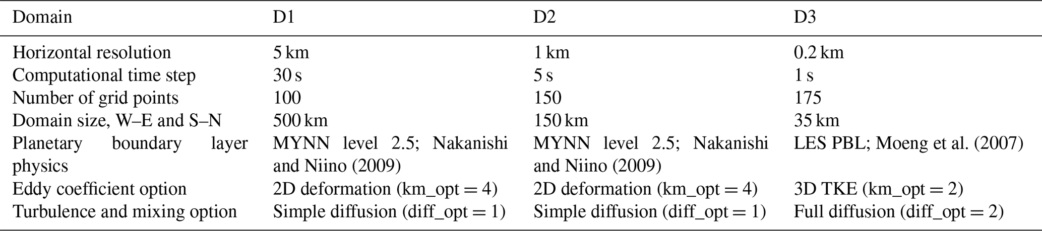
To investigate the influence of atmospheric turbulence and the resulting inhomogeneity in the propagation of exhaust plumes, we use WRF-ARW, the Advanced Research version of the Weather Research and Forecasting model (Skamarock et al., 2008). It is a well-established platform to investigate the transport of plumes (Zhao et al., 2019; Bhimireddy and Bhaganagar, 2018; Yver et al., 2013). The model configuration can be found in Table 2.

Table 2 WRF model configuration.

Considering typical source distances of the measurement crossings (see Table 1), in addition to the spread of the plumes (see Fig. A1), it is clear that our investigations need to be implemented with a horizontal resolution in the sub-kilometer range. To achieve this, we introduce three nested domains with the coordinates of the middle cooling tower as the center of the domains (see Fig. 5). The domain configurations can be found in Table 3. As meteorological initial and boundary conditions, operational ECMWF analysis data are used with a horizontal resolution of 9 km.

Figure 5 Location of three time-nested domains (black squares) of the WRF simulation. They are centered on the power plant Jänschwalde (red square). The domains have a side length of 500 (D1), 150 (D2), and 35 km (D3) and a horizontal resolution of 5 (D1), 1 (D2), and 0.2 km (D3). Vertically, 57 eta levels are introduced, ranking from the ground up to a top layer pressure of 200 hPa.

Table 3 Configuration of quadratic domains.

As suggested by Powers et al. (2017) we run the inner domain D3 as a large eddy simulation (WRF-LES). This makes it possible to resolve local turbulence (Moeng et al., 2007). Several studies show that WRF-LES is an adequate tool to model plume trajectories, in conjunction with turbulence and passive tracer dispersion (Nunalee et al., 2014; Nottrott et al., 2014).

Only the plume of the power plant is simulated without any CO₂ background field. WRF-ARW has the option to predefine a tracer variable $\text{tr}(t,x,y,z)$ which has the properties of a passive tracer, as used in Blaylock et al. (2017). It represents a 4D field of space-time. A detailed description of the calculation of simulated DAOD can be found in Appendix A. Therein Eq. (A3) is used to calculate the DAOD enhancement corresponding to the horizontal dispersion of the tracer, as shown in Fig. 6.

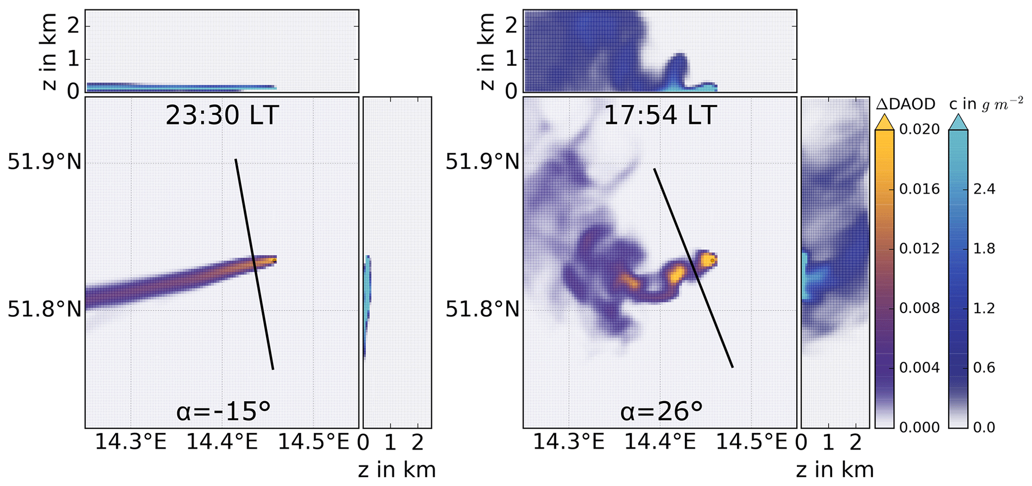
Figure 6 Exemplary snapshots of simulated exhaust plumes. The flight track of the virtual plume overflight is shown as a black line. At the top of the respective middle panels, the local time is given in Central European summer time (CEST, i.e., UTC+2), and at the bottom α denotes the local solar altitude. The first color bar represents the DAOD enhancement and refers to the respective middle panel, which shows the horizontal dispersion of the plume. The second color bar represents the mass per area and refers to the top and right panels, which show the vertical dispersion. In a corresponding measurement, DAOD enhancement values below 0.008 would not be distinguishable from noise and are therefore displayed in blue. Values higher than 0.01 exceed the noise and can be identified as plume enhancement in a real measurement. A ΔDAOD value of 0.02 corresponds to an enhancement of 4 % with respect to a background of 0.5 (cf. Fig. 3). The color maps follow the guidelines for a perception-based color map presented by Stauffer et al. (2015).

The WRF simulation provides a data output every 2 min. One virtual plume crossing is evaluated for each output time step at a point source distance of 1.5 km. This corresponds to our measurements (see Table 1). Since neither background field nor noise is simulated, it does not matter at which distance to the point source the virtual flyover takes place. Nevertheless, we try to match the virtual survey as closely as possible to real conditions. Just as in the real measurement, the virtual crossings are arranged perpendicular to the propagation direction of the plume (cf. Sect. 2.1). However, in a turbulent atmosphere, it is not trivial to precisely identify this direction of propagation. In this work, we consider the center of mass of the emitted tracers within a radius of twice the point source distance, i.e., 3 km. A connecting line between this center of mass and the point source corresponds to the propagation direction.

For the calculation of the virtually retrieved emission rate, the mean wind speed and direction are needed (see Eq. 3). To obtain these from the simulation, the following procedure is performed. First, for each data output step the horizontal wind components at the mean height of the plume are retrieved by vertical integration, weighted with tracer mass content. Second, the resulting 2D wind field is linearly interpolated onto the virtual flight path, yielding a 1D field with the horizontal wind components along the flight track. Last, the wind components are integrated and weighted with the DAOD along the flight track, resulting in the mean wind used for calculation.

5 Simulation results

WRF is able to simulate realistic plume dispersion. The DAOD enhancement values correspond to our measurements. Exemplary snapshots of the simulated plume during the course of a whole day can be found in Appendix A in Fig. A2. Additionally, an animated GIF of the simulated plume can be found under https://doi.org/10.5281/zenodo.4266513 (Wolff, 2020). In the nocturnal absence of solar irradiation, the turbulence decreases, leading to narrow, homogeneous plume dispersion within a laminar flow. The exhaust plume follows Gaussian behavior, as depicted in Fig. 6 at 23:30. Contrary to this, we find boundary layer turbulence during daytime.

Strong solar heating of the surface generates convective air masses, which in turn cause a cascade of eddies. Consequently, locally reverse and counter-gradient flow, i.e., flow opposite to the main wind direction, emerges. This results in local puffs of above-average column concentration enhancements within the exhaust plume, while eddy-generated local flow in the same direction as the ambient wind causes constrictions of lower column concentrations in a plume (Stull, 1988). Such plume structures deviate from Gaussian behavior, as can be seen in Fig. 6 at 17:54.

Locally increased CO₂ column concentration results in a high value in the integrated enhancement A in contrast to an overflight over a constriction. Following Eq. (3) this corresponds to a high value of the emission rate q. It should also be stressed that the spatial extent of such puffs is smaller than that of complementary constrictions. Therefore, a skewed distribution of the retrieved emission rates is to be expected, as Fig. 7 confirms.

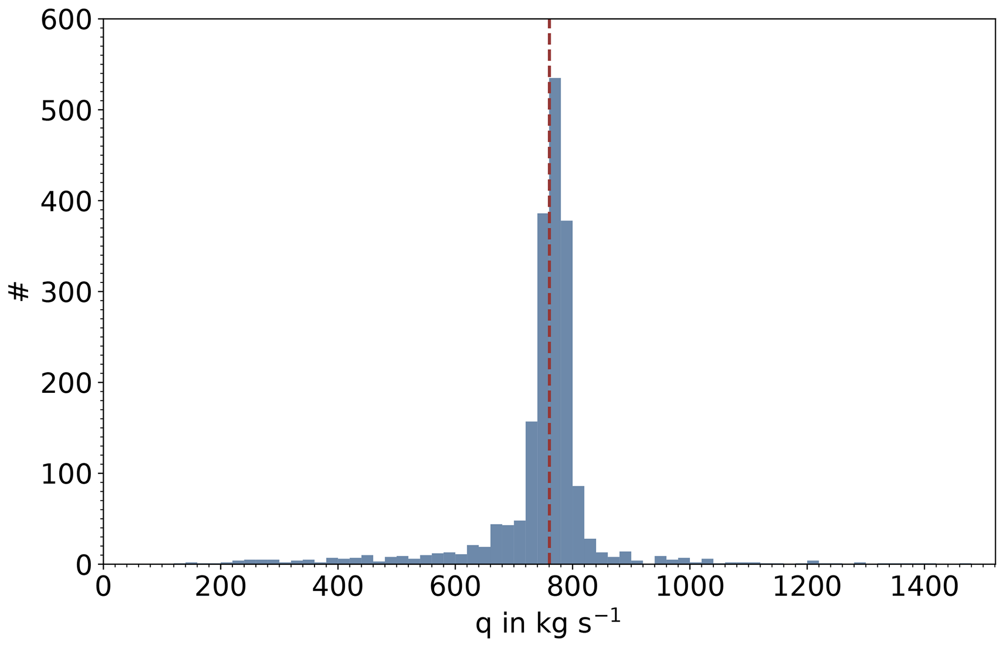
Figure 7 Histogram of virtually retrieved emission rates. The histogram shows a slightly skewed distribution towards smaller emission rates than the input emission rate (dashed red line). It depicts all 1980 emission rates retrieved over 66 simulated hours between 12:00 UTC on 21 May and 06:00 UTC on 24 May.

On 23 May 2018, four measurement flyovers of the power plant Jänschwalde took approximately 1 h, as presented in Sect. 3. As spin-up we discard the first 6 h of the simulation (see Table 2). That is 66 h of simulation, which leaves us with a total of 1980 virtual plume flyovers. The corresponding results of the emission rate, which are calculated using Eq. (3), are displayed as a histogram in Fig. 7 and as a time series in Fig. 8a.

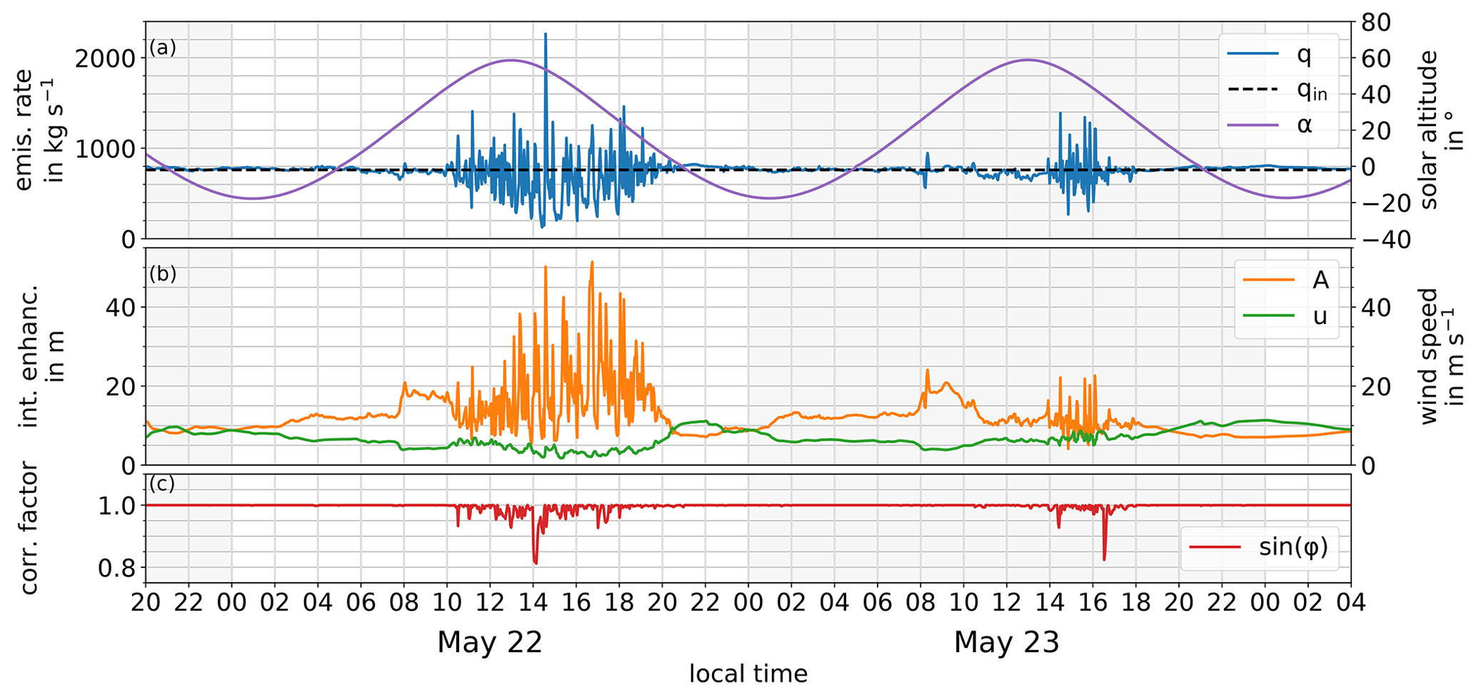
Figure 8 Virtual overflight results in the course of the day. In (a) it can be seen that rising solar altitude α entails turbulence. Especially midday turbulence causes deviations in the retrieved emission rate q from the input emission rate q_in. In (b) the integrated enhancement A shows equivalent behavior, while the variations in wind speed u are comparatively small. It is during the midday turbulence that the virtual flight tracks are not exactly perpendicular to the instantaneous wind direction at the plume crossing, which becomes apparent in the correction factor sin (φ) in (c). In the night hours, as well as the morning, the retrieved emission rates agree very well with the input emission rate q_in. The wind speed u surpasses the threshold value of 2 m s⁻¹ at all times.

In Fig. 8a it can be seen how the diurnal course of solar altitude α influences the retrieved emission rates q. The random occurrence of inhomogeneities in the plume propagation, caused by local turbulence, leads to large variations in the results of successive crossings. Turbulence lags behind solar altitude because the surface needs time to heat up. It is also apparent that the emission rate deviations vary from day to day, both in intensity and in dwell time.

The implications for the measurement results can be reduced by averaging over a multitude of retrieved emission rates. Next, we investigate how often the exhaust plume must be surveyed to achieve a mean emission rate with satisfactory accuracy. From experience with the Jänschwalde measurement presented in Sect. 3, as well as other point source measurements during the CoMet campaign which are not presented in this work, we assume a time delay in the range of 6 to 18 min between two successive crossings. With typical wind speeds in the range of 5–8 m s⁻¹ and spatial scales of puffs and constrictions of about 1–2 km, our range of time delay exceeds the residence time of coherent plume structures, thus preventing repeated measurements of identical air masses. The model setup provides one measurement every 2 min, resulting in a vast number of permutations of successive virtual crossings available for merging (see Table A1). For each of these permutations, a mean value is calculated, which is then compared with the initiated emission rate q_in. To evaluate the turbulence-induced inhomogeneity in the daily course, we compare 2 h time frames. We execute a total of 60 virtual overflights in such a 2 h time frame. The number of possible permutations increases exponentially to 5000 if four crossings are merged and even on to 312 500 if seven crossings are merged (see Table A1). This high number of permutations is based on the identical 60 single crossing emission rates, which are displayed in the purple box–whisker plots for single crossings in Fig. 9.

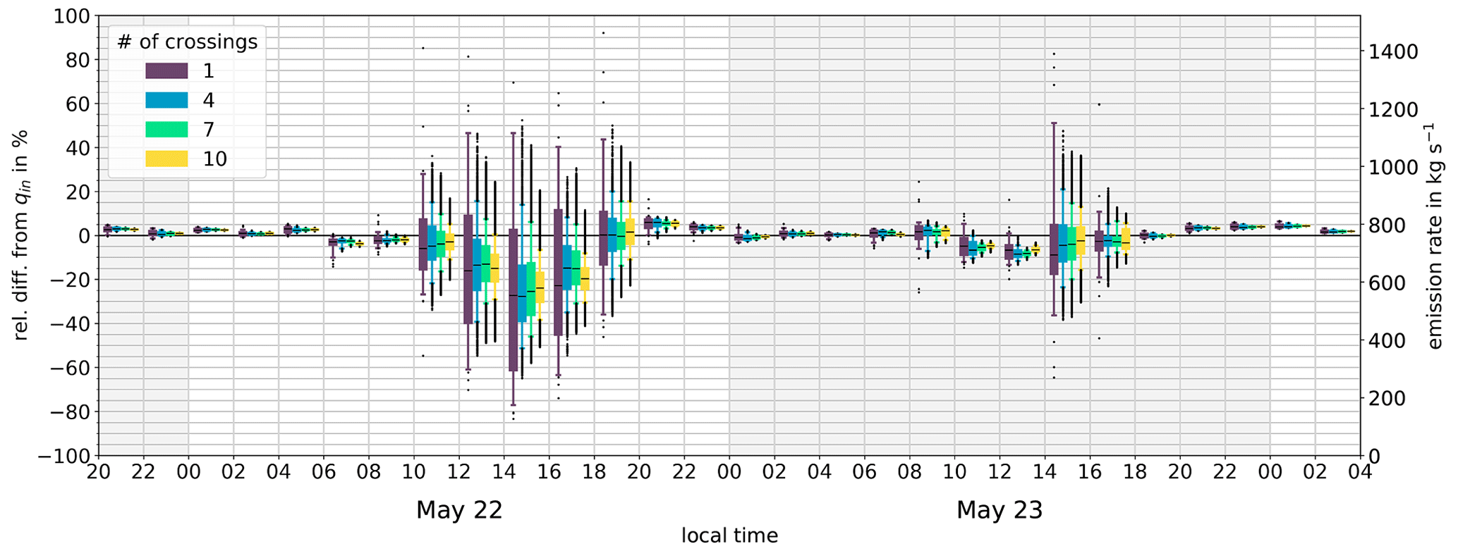
Figure 9 Box–whisker plot of the relative difference to the input emission rate q_in within 2 h time frames. The right axis shows the associated retrieved emission rates. The width of the distribution decreases with a higher number of crossings. For all time frames it can be stated that with an increasing number of merged crossings, the width of the distribution decreases. The largest differences to q_in are observed in the afternoon. Different colors represent a different number of virtual crossings merged for averaging. The inner boxes range from the first to the third quartile, thus containing 50 % of the values. The median is marked within as a black dash. The upper whisker is drawn up to the 95th percentile, while the lower whisker is drawn to the 5th percentile. Consequently, 90 % of the values are in between the two whiskers. All values outside the whiskers are outliers and plotted as dots.

Figure 9 presents the resulting distribution of this relative difference to the input emission rate as a box–whisker plot. The spread of the respective box–whisker plot is an indicator of turbulence. It is evident that with an increasing number of overflights merged for averaging, the spread of the relative differences decreases, while the measurement precision increases. A high emission rate measured by a single overflight scanning a puff is compensated for if the subsequent overflight measures a lower emission rate. With a higher number of overflights averaged, it is more likely to measure both high- and low-concentration air masses. Yet, although the precision can be improved by increasing the number of overflights, even for 10 overflights it is inferior to the precision of nighttime measurements. Additionally, not only the precision but also the accuracy is compromised during times of strong turbulence, i.e., in the afternoon. As mentioned above, the spatial extent of turbulence-induced puffs is smaller than the one of the complementary constrictions. Therefore, such puffs are likely to be less frequent and only partially scanned when measured at a low sampling frequency. Consequently, the retrieved emission rates will be biased low. This is an effect that occurs especially during strong turbulence. In Fig. 9 a strongly turbulent day (22 May) is compared to a less turbulent day (23 May). Both precision and accuracy are superior on a less turbulent day.

In contrast, the night hours show little turbulence and high precision. Even with a single overflight, small differences to the true emission rate are to be expected. Here, a higher number of overflights will only cause minor improvements. At this point, it should be mentioned that the representation of nightly plume propagation must be critically reviewed. The plume height decreases so much that the propagation takes place only in the lowest four model layers. The fact that a bias of approx. ±5 % remains at night is not surprising from this point of view. This study should therefore be understood as a qualitative assessment. The key finding is that avoiding situations of high turbulence brings an enormous improvement for both precision and accuracy. Even with a significantly higher number of measurement overflights, a comparable improvement cannot be attained.

6 Discussion

Regarding the lidar measurements during the CoMet campaign on 23 May 2018, we find that the mean emission rate, derived from repeated plume overflights, is in rough agreement with the average emission reported by the power plant operator for the year 2017. The cross-sectional flux method is straightforward to apply. The exhaust plume generates column enhancements in the differential absorption optical depth (DAOD), with a good signal-to-noise ratio, on the order of 10 %. The product of enhanced column concentration integrated along the flight track and mean wind speed, provides the flux through the lidar cross section at the instant of the overflight. This instantaneous flux of an individual overflight measurement can be determined with an error ranging between 8 %–10 %. This error is mainly driven by uncertainties in the integrated enhancement, the mean differential absorption cross section, the mean relative wind direction, and the mean horizontal wind speed. On average, we find that $\mathrm{2}/\mathrm{10}$ of the flux error can be attributed to uncertainty in the determination of the integrated enhancement, i.e., the integrated enhancement of the DAOD signal, which is the only parameter that needs to be derived from the IPDA lidar measurement. A total of $\mathrm{1}/\mathrm{10}$ can be attributed to the uncertainties in the mean differential absorption cross section of CO₂ and the relative wind direction taken together. The main source of error, however, is the mean horizontal wind speed with a contribution of $\mathrm{7}/\mathrm{10}$. This highlights the need for more accurate wind information. Future studies will examine CHARM-F measurements in the Upper Silesian Coal Basin to determine CH₄ emissions from coal mines. In this area, ground-based Doppler wind lidars have been installed. It is expected that nudging the simulation towards the wind soundings will result in an improvement of the wind vector estimation, ultimately reducing the overall error in the flux determination.

It is necessary to distinguish between instantaneously measured flux and actual emission rate. In theory, an exhaust plume behaves Gaussian on average, and the mean emission rate of the point source lies within the error range of the instantaneously measured fluxes. Contrary to this, our overflights reveal large variations between the individually retrieved instantaneous fluxes which cannot be attributed to measurement uncertainties. These variations do not occur because the measurement error increases, but because plume segments with varying CO₂ content are probed. The actual measurement error is minor compared to these variations (cf. Table 1). As described in Sect. 5, strong solar heating causes turbulence, which forces the plume to deviate from Gaussian behavior. This deviation can be restricted by averaging over multiple instantaneous fluxes, as the results from our measurement flights suggest.

To analyze this effect in more detail, we employ the atmospheric transport model WRF in a high-resolution large eddy simulation (LES) setup. We find that the model simulates realistic plume dispersion. Typical DAOD values, as well as turbulence-induced distortions, show the same order of magnitude as our measurements. However, as we evaluate only four overflights in the measurement, we cannot make any statement about the absolute accuracy of the simulation, which is also not the intention of this work. Qualitatively, the simulation provides the following insights. During the night the plumes are weakly distorted and have a Gaussian shape because laminar flow dominates. Over the course of the day, turbulence increases, reaching its peak in the mid-afternoon and distorting the plumes to non-Gaussian shapes. Thus, with increasing turbulence, a larger number of crossings is required for averaging in order to obtain sufficient emission rate precision. According to our simulation, nighttime measurements require fewer overflights. Under such conditions, even a single instantaneous cross-sectional flux measurement yields an accuracy of up to ∼95 %. In cases of very pronounced turbulence (i.e., in the afternoon), even an impractically high number of overflights will neither reach the precision nor the accuracy of a single nighttime overflight.

At this point, we cannot derive any limits for solar altitude or local times that should be avoided as the simulation reveals that the turbulence intensity varies from day to day (see Figs. 8 and 9). Generally, we find that the most significant turbulence occurs in the afternoon. For future campaign planning, we recommend to also perform measurements at night or in the morning, which is possible with lidar.

7 Conclusions

The present study continues the investigations by Amediek et al. (2017) on the quantification of fluxes of local greenhouse gas emission sources using the integrated path differential absorption (IPDA) lidar CHARM-F and the cross-sectional flux method. While the preceding study was concentrated on CH₄ emissions from hard coal mines, here, we exploit the results from the CoMet campaign in 2018. We investigate CO₂ plume overflights of the coal-fired power plant Jänschwalde, conducted to quantify its emission rate and to assess how accurately the cross-sectional flux method can be applied. Since CHARM-F measures both greenhouse gases simultaneously, our findings also apply to isolated CH₄ point sources.

With regard to cross-sectional flux measurements, the current work suggests avoiding mid-afternoon periods of strong turbulence. On the one hand, this is because the uncertainties in the wind speed are most pronounced at these times, being the major source of error in a single measurement. On the other hand, this is due to the distortions of exhaust plumes in a turbulent wind field, which lead to substantial deviations from Gaussian plume dispersion. Under strong turbulence, the cross-sectional flux method cannot provide an accurate measurement of the emission rate, not even in the average of a vast number of overflights. Therefore, measurement flights performed during nighttime are beneficial. In this respect, intrinsic independence from solar irradiation is a clear advantage of active remote sensing over passive approaches. Whenever sunlight is needed to perform the measurement, less turbulent conditions, for example in the morning after sunrise or winter, should be preferred. Further, it should be pointed out that, with a lidar, cross-sectional plume measurements can also be performed over water bodies whose detrimental reflective properties often impede the use of passive remote sensing (Gerilowski et al., 2015; Krautwurst et al., 2021; Larsen and Stamnes, 2006). Therefore, plumes from offshore installations can also be addressed with this approach.

Independent of the location of the point source, there are restrictions regarding the adequate distance of a plume overflight to the point source. We report that at a point source distance of more than 4.6 km no enhancement is visible and therefore no plume detection can be performed. In addition to that, we find that the uncertainty of the mean differential absorption cross section increases with a larger vertical extension of the plume which correlates with distance. At a point source distance of 1.5 km, this uncertainty is negligible. Concerning the detectability of the plume, we can locate distinct enhancements at a distance of 1.5 km. Nevertheless, the closer to the point source the overflight takes place, the more constrained the plume and consequently the more pronounced the column enhancement is. It must be considered, however, that the horizontal extension is also smaller, and thus fewer data points lie within the plume. In the case of CHARM-F, this can be compensated for by a higher repetition rate.

8 Outlook

Apart from the CHARM-F measurements, the CoMet campaign also saw the deployment of other airborne instruments to measure atmospheric CH₄ and CO₂, supported by a variety of ground-based, in situ, and remote sensing instruments. They were predominantly based in the vicinity of one of the major hot-spot regions of CH₄ emissions in Europe, the Upper Silesian Coal Basin (USCB). Investigations of local and regional CH₄ emissions from this region are, in view of the preparation for the upcoming MERLIN mission, a particular field of interest. The possibility to synergistically use active remote sensing (lidar), passive spectrometry, and in situ measurements supported by modeling activities allows for unique cross comparisons, which are beyond the scope of the present paper. Such cross comparisons will be the subject of subsequent investigations, as well as other HALO measurement flights, as it flew along latitudinal trajectories, performed regional survey flights (e.g., over Mount Etna), and also probed the local plume of not only Jänschwalde but also Bełchatów in Poland, which is considered Europe's largest coal-fired power plant in terms of CO₂ emission. The measured data can make an important contribution to the validation of existing satellite missions (e.g., Sentinel-5P, GOSAT). Further aircraft campaigns (e.g., CoMet-2.0) are foreseen which will provide additional opportunities for methodical refinements, including advancements in model-measurement synergies.

Appendix A

Figure A1 Figures of individual HALO crossings on 23 May 2018. Individual transects listed in Table 1. The black line shows a 0.2 km (64 data points) running mean, as first presented in Fig. 3. Vertical red lines mark the smallest data extract used for the Riemann sum, as described in Sect. 3.

Calculation of simulated DAOD

At the initialization position of the power plant, the value of the tracer variable tr is increased by the value 1 at each time step. In this study, it is defined only in the inner domain D3.

$$\begin{array}{}\text{(A1)}& \mathrm{tr}\left(t+\mathrm{\Delta }t,x,y,z\right)=\mathrm{tr}\left(t,x,y,z\right)+\mathrm{1}\end{array}$$

Here, Δt corresponds to the computational time step of the third domain, i.e., 1 s (Table 3). At the same time the tracer is distributed in the domain D3 by advection and turbulent dispersion. The corresponding mass concentration $c(t,x,y,z)$ at any grid point $x,y,z$ at time t is obtained as follows:

$$\begin{array}{}\text{(A2)}& c\left(t,x,y,z\right)=\mathrm{tr}\left(t,x,y,z\right)\cdot {\displaystyle \frac{q_{\text{in}}\cdot \mathrm{\Delta }t}{\mathrm{\Delta }x\cdot \mathrm{\Delta }y\cdot \mathrm{\Delta }z(t,x,y,z)}}.\end{array}$$

For the input emission rate q_in a constant value of 760 kg(CO₂) s⁻¹ (24.0 Tg(CO₂) yr⁻¹) is initialized, which corresponds to the total annual emissions for the year 2017 reported to the European Environment Agency by the operators (E-PRTR, 2020). The horizontal size of a grid point Δx and Δy are temporally and spatially constant (0.2 km). The vertical layer size $\mathrm{\Delta }z(t,x,y,z)$ corresponds to the spatial distance between two model levels. In the simulation this distance is computed in pressure coordinates and depends on all four dimensions. Since the pressure varies only slightly between successive time steps, the temporal dependence of Δz is small. At locations with flat topography the dependence of Δz on the horizontal coordinates x and y is also small, and at locations with large topographic changes (e.g., steep slopes) the dependence is more significant. The product $\mathrm{\Delta }x\cdot \mathrm{\Delta }y\cdot \mathrm{\Delta }z(t,x,y,z)$ corresponds to the volume of the respective grid box. Within this volume the value of the tracer variable and thus the concentration is constant.

In order to compare the simulated data with an IPDA lidar measurement, the concentration array must be summed up vertically and multiplied by the quotient of the mean differential absorption cross section and the molecular mass.

$$\begin{array}{}\text{(A3)}& \begin{array}{rl}{\text{DAOD}}_{\text{wrf}}\left(t,x,y\right)& ={\displaystyle \frac{\stackrel{\mathrm{‾}}{\mathrm{\Delta }\mathit{\sigma }}}{M}}\cdot \sum _{j=\mathrm{1}}^{j_{\text{top}}}c\left(t,x,y,z_j\right)\\ & \cdot \mathrm{\Delta }{z}_j(t,x,y,z)\end{array}\end{array}$$

The index j marks the respective vertical layer. Consequently, $j\in \left\{\mathrm{1},\mathrm{56}\right\}$ applies, and z_j is defined as corresponding to the lower edge of the respective layer.

Figure A2 Exemplary snapshots of simulated DAOD. Exemplary snapshots of simulated plume and virtual flight track. At the respective tops, local time is given in Central European summer time (CEST, i.e., UTC+2), and at the bottom α denotes the local solar altitude. The daily solar irradiation causes a deep, convective boundary layer with turbulent plume dispersion within. In the nocturnal absence of solar irradiation, the boundary layer shrinks, leading to narrow, homogeneous plume dispersion within a laminar flow. Every 2 min a virtual measurement is performed yielding 60 measurements within a time frame of 2 h. One representative snapshot within the 2 h time frame is shown. Some snapshots show disjointed exhaust plumes. This is due to vertical wind shearing and the resulting different vertical advection directions.

Table A1 Number of possible permutations of successive virtual crossings used for averaging.