Estimation of the error covariance matrix for IASI radiances and its impact on the assimilation of ozone in a chemistry transport model

In atmospheric chemistry retrievals and data assimilation systems, observation errors associated with satellite radiances are chosen empirically and generally treated as uncorrelated. In this work, we estimate inter-channel error covariances for the Infrared Atmospheric Sounding Interferometer (IASI) and evaluate their impact on ozone assimilation with the chemistry transport model MOCAGE (Modèle de Chimie Atmosphérique à Grande Echelle). The method used to calculate observation errors is a diagnostic based on the observation and analysis residual statistics already adopted in many numerical weather prediction centres. We used a subset of 280 channels covering the spectral range between 980 and 1100 cm⁻¹ to estimate the observation-error covariance matrix. This spectral range includes ozone-sensitive and atmospheric window channels. We computed hourly 3D-Var analyses and compared the resulting O₃ fields against ozonesondes and the measurements provided by the Microwave Limb Sounder (MLS) and by the Ozone Monitoring Instrument (OMI).

The results show significant differences between using the estimated error covariance matrix with respect to the empirical diagonal matrix employed in previous studies. The validation of the analyses against independent data reports a significant improvement, especially in the tropical stratosphere. The computational cost has also been reduced when the estimated covariance matrix is employed in the assimilation system, by reducing the number of iterations needed for the minimizer to converge.

1 Introduction

Ozone is an important trace gas that plays a key role in the Earth’s radiative budget (Iglesias-Suarez et al., 2018), in the chemical processes occurring in the atmosphere, and in climate change (United Nations Environment Programme (UNEP) 2015). Tropospheric ozone also behaves as a pollutant with negative effects on vegetation and human health (UNEP2015, 2015). The stratospheric ozone is, nevertheless, a vital component of life on the Earth since it protects the biosphere from harmful ultraviolet solar radiation (WMO, 2014). Therefore, monitoring the atmospheric ozone has been a subject of numerous research studies and projects (e.g. Monitoring Atmospheric Composition and Climate (MACC) project (Inness et al., 2013)). O₃ surveillance is carried out through numerical forecast models and observational systems. The information arising from these two sources is, thereafter, combined with the data assimilation techniques to improve the system state and forecasts.

Remote soundings from satellites are an essential component of an observational network (Clerbaux et al., 2009). Several remote sensors relying on thermal emission of the Earth and the atmosphere have demonstrated their ability to provide appropriate information for total columns or vertical profiles of atmospheric gases such as water vapour, carbon dioxide, and ozone (Clarisse et al., 2008; Clerbaux et al., 2009; Irion et al., 2018). Furthermore, the role of thermal infrared sounders does not typically end at the monitoring of atmospheric gases. A large number of applications have taken advantage of these measurements: the estimation of meteorological parameters (clouds, temperature, and humidity) and climate change studies (e.g. MacKenzie et al., 2012). The Infrared Atmospheric Sounding Interferometer (IASI) is one of these thermal infrared sounders on board Metop-A which provides global-scale observations for a series of key atmospheric species (Clerbaux et al., 2009).

Data assimilation has been introduced relatively recently in atmospheric chemistry, in the stratosphere (Fisher and Lary, 1995) and for the troposphere (Elbern et al., 1997). Chemical fields estimated by chemistry transport models (CTMs) are combined with observations to construct a more accurate description of the atmospheric composition evolution (Lahoz et al., 2007). Numerous studies have been conducted assimilating satellite retrievals of ozone (Emili et al., 2014; Massart et al., 2009). However, the quality of analyses might be influenced by the prior information used for the retrievals. A recent study (Emili et al., 2019) attempted to assimilate satellite radiances directly in a CTM to overcome this issue. In chemical assimilation systems that assimilate radiances directly, but also in most of the current satellite retrieval algorithms (Dufour et al., 2012), the observation errors are empirically adapted from the nominal instrumental noise and assumed to be uncorrelated. This assumption is questionable since we use a radiative transfer model that may introduce similar errors among different spectral channels (Bormann et al., 2010). In other words, an error dependency between channels of the band used is likely to be introduced. The inter-channel error correlations might originate from observation operator errors. They can also arise from the instrument calibration and some practices of quality control (Bormann et al., 2010; Waller et al., 2016; Geer, 2019). The representation errors (Janjić et al., 2018) may also introduce correlations. Liu and Rabier (2003) have shown that the assimilation can lead to sub-optimal analysis errors when observation-error correlations are neglected.

The weight given to the observation in the assimilation process is determined by its error covariance matrix R. Therefore, its estimation plays a crucial role in the assimilation results. While most chemical assimilation systems assume the observation error to be uncorrelated, many numerical weather prediction (NWP) centres have estimated non-diagonal observation-error covariances for satellite instruments such as the Atmospheric Infrared Sounder (Garand et al., 2007; Bormann et al., 2010), IASI (Stewart et al., 2009; Bormann et al., 2010; Weston et al., 2014; Campbell et al., 2017; Bathmann et al., 2020), and the Spinning Enhanced Visible and Infrared Imager (Waller et al., 2016). The results found in the literature for the meteorological applications incite us to account for a correlated observation error for the chemical assimilation system as well. Indeed, the studies mentioned above show that the inter-channel observation errors are correlated and taking such correlated errors into account in the assimilation leads to improved analysis accuracy. Additionally, Emili et al. (2019) have highlighted some issues when assimilating radiances in a chemistry transport model (increase in the ozone analysis errors compared to the control simulation at some specific altitudes), which might be due to too simplistic observation errors. The main objective of this study is, thus, to improve the ozone analysis accuracy within a chemistry transport model, by means of using more realistic observation-error covariances for IASI ozone-sensitive channels.

The estimation of R is not straightforward, but a number of statistical methods are already evaluated in the literature. Desroziers et al. (2005) have proposed an estimation based on the observation and analysis residual statistics. By assuming Gaussian errors and no correlations between observation and background errors, the error covariance matrix is provided by the statistical average of observation-minus-background times the observation-minus-analysis residuals. This method has been used in many studies to estimate the observation errors and inter-channel error correlations (Garand et al., 2007; Weston et al., 2014; Bormann et al., 2016; Tabeart et al., 2020; Coopmann et al., 2020).

In the present work, we estimate observation errors and their inter-channel correlations for IASI using the Desroziers method. We evaluate, then, their impact on ozone assimilation in a CTM (MOCAGE). The paper is organized as follows. The CTM, the radiative transfer model, the assimilation algorithm, the data, and the experimental framework are described in Sect. 2. The estimation of R is discussed in Sect. 3. Then, the impact on data assimilation is reported in Sect. 4, and validation against independent data is discussed in Sect. 5. Finally, the summary and conclusions are given in the last section.

2 Methods and data

2.1 Methods

2.1.1 Chemistry transport model

MOCAGE (Modèle de Chimie Atmosphérique à Grande Echelle) is the CTM used in this study. It is a three-dimensional CTM providing the space and time evolution of the chemical composition of the troposphere and the stratosphere. Developed by Centre National de Recherches Météorologiques (CNRM) at Météo France (Josse et al., 2004), it was used for a large number of applications such as satellite ozone assimilation (Massart et al., 2009; Emili et al., 2014), climate (Teyssèdre et al., 2007), and air quality (Martet et al., 2009). MOCAGE provides a number of optional configurations with varying domains, geometries, and resolutions, as well as multiple chemical and physical parametrization packages.

A global configuration with a horizontal resolution of 2^∘ and 60 hybrid levels from the surface to 0.1 hPa was used. The vertical resolution goes from about 100 m in the boundary layer to about 500 m in the free troposphere and to almost 2 km in the upper stratosphere. MOCAGE is forced by meteorological fields from numerical weather prediction models such as the Météo France global model ARPEGE (Action de Recherche Petite Echelle Grande Echelle, (Courtier et al., 1991)), limited-area model AROME (Application de la Recherche à l'Opérationnel à Méso-Echelle), and ECMWF NWP model and assimilation system (Integrated Forecast System, IFS) for air quality predictions and ARPEGE-Climat (Déqué et al., 1994) for climate simulations. In our study, the ECMWF IFS meteorological forecasts fields are used. For the chemical scheme, we adopted RACMOBUS, which bundles the stratospheric scheme (Lefèvre et al., 1994) and the tropospheric scheme (Stockwell et al., 1997), including about 100 species and 300 chemical reactions.

2.1.2 Radiative transfer model

Remote sensing instruments measure, within a certain wavelength range, the intensity of electromagnetic radiation passing through the atmosphere (radiances). Radiative transfer models are used to simulate the radiation measured by the satellite as a function of atmospheric state, to be able to compare the model state to the observed radiances.

In our study, IASI radiances are simulated using the radiative transfer model RTTOV (Radiative Transfer for TOVS), which was initially developed for TOVS instruments (Saunders et al., 2018). Giving an atmospheric profile of temperature, water vapour, and, optionally, trace gases, aerosols, and hydrometeors, together with surface parameters and a viewing geometry, RTTOV simulates radiances in the infrared and microwave spectrum. For IASI, it can reproduce radiances with an accuracy of less than 0.1 K (Matricardi, 2009). In this paper, we use the same version used by Emili et al. (2019), i.e. version 11.3 (Saunders et al., 2013). The radiative transfer computations are performed in clear-sky conditions and aerosols are neglected. The surface skin temperature, 2 m temperature, 2 m pressure, and 10 m wind vector are taken from IFS forecasts. The land surface emissivity is based on the RTTOV monthly thermal infrared (TIR) emissivity atlas (Borbas and Ruston, 2010), and the Infrared Surface Emissivity Model (ISEM) (Sherlock, 1999) is used over the sea. Other chemical variables (CO₂, CH₄, CO, N₂O) were set to the reference profiles of RTTOV.

2.1.3 Assimilation algorithm

The variational data assimilation system of MOCAGE was developed jointly by CERFACS and Météo France in the framework of the European project ASSET (Assimilation for Envisat data) (Lahoz et al., 2007). It has been used in several studies such as chemical data assimilation research (Emili et al., 2014; Massart et al., 2009), aerosol data assimilation (Sič et al., 2015), and tropospheric–stratospheric exchange using data assimilation (El Amraoui et al., 2010). The MOCAGE data assimilation system is flexible and allows multiple assimilation options, for example, the choice of the variational method (3D-Var, 4D-Var), the representation of the background-error covariance, and the type of observation assimilated. It is also used to produce operational air quality analyses for the European project CAMS (Marécal et al., 2015).

The background-error covariance matrix is divided into two distinct parts, the diagonal matrix of the standard deviations and the correlation matrix. The latter, allowing the spatial smoothing of the assimilation increments, is modelled through a diffusion operator (Weaver and Courtier, 2001).

The 3D-Var implementation has been used with hourly assimilation windows. The variational cost function is minimized using the BFGS (Broyden–Fletcher–Goldfarb–Shanno) algorithm (Liu and Nocedal, 1989). The system is preconditioned with the square root of the B matrix. The control vector includes only skin surface temperature (SST) and ozone.

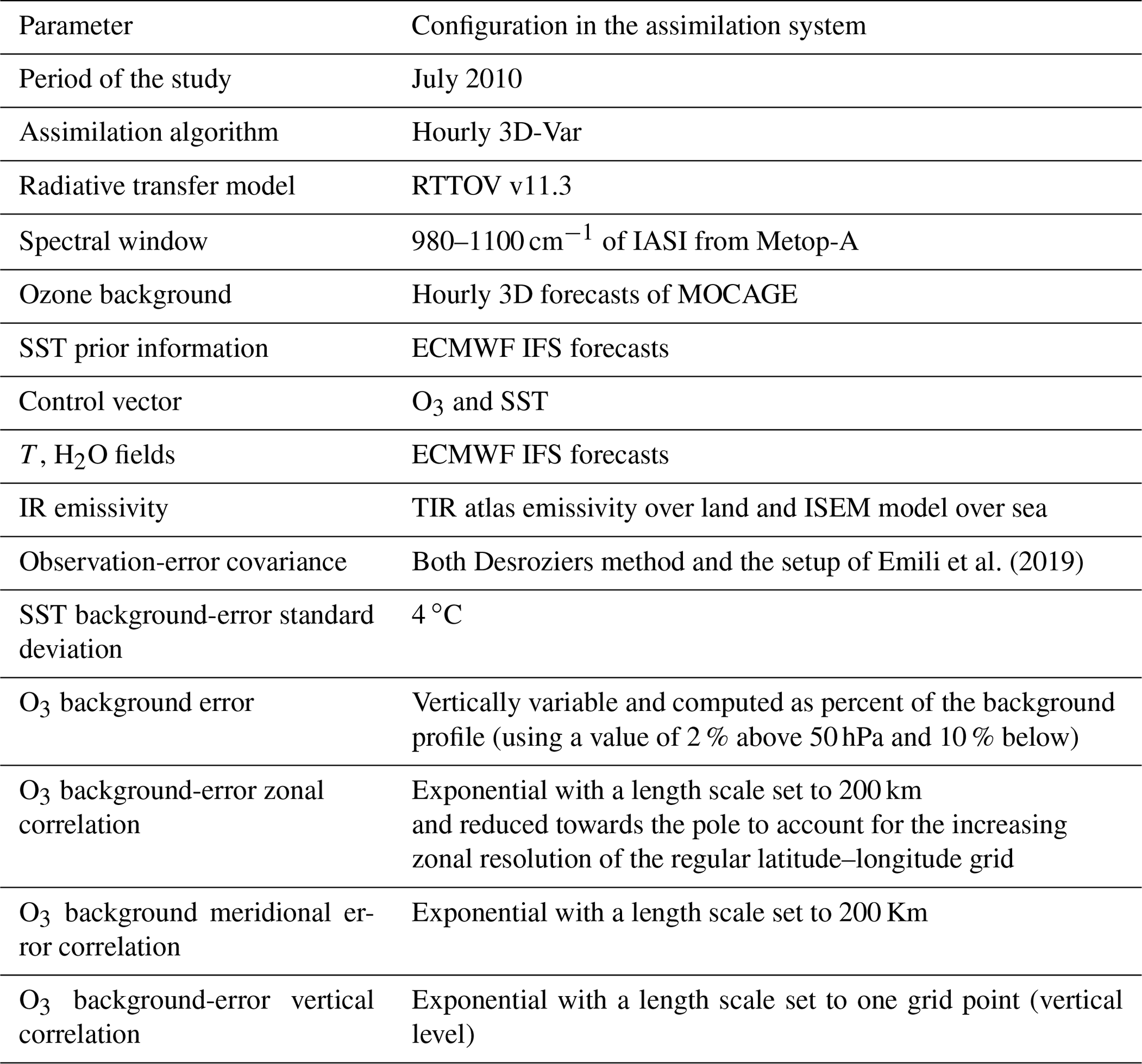
As we mentioned before, the aim of this work is to evaluate the impact of the estimated observation-error covariances on the ozone analysis. Hence, in order to be able to compare our results to those that have already been discussed and validated, we kept exactly the same configurations as those used in Emili et al. (2019) in terms of model, radiative transfer, and assimilation algorithm parameters. The summary of these configurations is given in Table 1.

2.2 Data

2.2.1 IASI

IASI is one of the instruments operating on board the polar-orbiting satellite Metop-A, B, and C launched by the European organization for the Exploitation of Meteorological Satellites (EUMETSAT). It is based on a Fourier transform spectrometer (FTS) and measures the spectrum emitted by the Earth atmosphere system in the spectral range between 645 and 2760 cm⁻¹ (3.62 and 15.5 µm) with a resolution of 0.5 cm⁻¹ after apodization, with a spectral sampling of 0.25 cm⁻¹. IASI scans the Earth up to an angle of 48.3^∘ on both sides of the satellite track. The cross-track is observed in 30 successive elementary fields of view, each composed of four instantaneous fields of view corresponding to a 12 km diameter footprint on the ground (Clerbaux et al., 2009). The swath width on the ground is 2200 km, which provides global Earth coverage twice a day. The measurements provide information on atmospheric chemistry compounds such as O₃, surface properties (skin surface temperature, SST), and meteorological profiles (humidity and temperature).

For this study, a subset of 280 channels covering the spectral range between 980 and 1100 cm⁻¹ was used. The channel selection is inherited from IASI Level 2 O₃ retrievals (Dufour et al., 2012; Emili et al., 2019). L1c data have been downloaded from the EUMETSAT Earth Observation data portal (https://eoportal.eumetsat.int, last access: 1 May 2020) in NetCDF format. Data files also contain the co-located land–sea mask and cloud fraction values, obtained from the Advanced Very High Resolution Radiometer (AVHRR) measurements, also on board Metop-A.

2.2.2 MLS

The Microwave Limb Sounder (MLS) provides vertical profiles of several chemical components, by measuring the microwave thermal emission from the limb of Earth's atmosphere (Waters et al., 2006). More than 2500 vertical profiles are observed daily, including trace gases with a vertical resolution of approximately 3 km. Several studies benefited from MLS products, notably the ozone profiles in assimilation experiments (Emili et al., 2014; Massart et al., 2009), thanks to its low bias in the stratosphere (<5 %) (Froidevaux et al., 2008).

In our study, we use the ozone profiles retrieved from MLS (V4.2 Products) as independent data to validate our results. The data have been downloaded from the Goddard Earth Sciences Data and Information Services Center (GES DISC) web portal (https://disc.gsfc.nasa.gov, last access: 1 May 2020).

2.2.3 OMI

The Ozone Monitoring Instrument (OMI) is a nadir-viewing, ultraviolet–visible (UV-VIS) spectrometer (Levelt et al., 2018). It provides complete global maps of total column ozone on a daily basis. The OMI ozone data record starts in October 2004, shortly after the launch of Aura (McPeters et al., 2015). The total column averaged over the month of the study (July 2010), resulting from the OMI-TOMS version 8 algorithm (Bhartia, 2002), is used here to validate the results of the assimilation experiments.

2.2.4 Ozonesondes

Ozonesondes are in situ instruments carried by a radiosonde continuously transmitting the measurements as it ascends. The profiles of O₃ are provided up to an altitude that often exceeds 30 km (Jiang et al., 2007) with a vertical resolution of 150–200 m. They have been used for several applications such as validating satellite products (Jiang et al., 2007). In our study, vertical profiles of ozone, collected and distributed by the Word Ozone Ultraviolet Radiation Data Centre (http://www.woudc.org, last access: 1 May 2020), are used to validate the model simulations.

2.3 Setup of the numerical experiments

The main purpose of this study is to estimate the IASI observation-error covariances and verify their impact on the quality of the ozone assimilation results. The setup of the experiment in terms of the period of the study, the model configuration, the choice of assimilated observations, and the background-error covariance matrix is reported in Table 1. The observation-error covariance matrix will be discussed in the results section (Sect. 3).

The model was initialized with a zonal climatology, and the spin-up time used is 1 month (June 2010). Then, our simulations were performed for the month of July 2010. The ozone forecast-error standard deviation was assumed to be proportional to the ozone concentration. In fact, Emili et al. (2019) have evaluated the standard deviation of the free model simulation against independent data (profiles from ozonesondes and MLS), and they found a small free forecast error in the stratosphere, larger error in the free troposphere, and the highest error close to the tropopause. This strategy was adopted previously by many studies (Emili et al., 2014; Peiro et al., 2018; Emili et al., 2019). Emili et al. (2014) and Peiro et al. (2018) have used a percentage of 15 % in the troposphere and 5 % in the stratosphere. In this study, we have adopted a detailed chemical scheme (discussed in Sect. 2.1.1). This scheme was shown to reduce the model bias compared to the scheme used in Emili et al. (2014) and Peiro et al. (2018) (see Fig. 4 in Emili et al., 2019). Hence, we chose the same background error as in Emili et al. (2019): 2 % of the O₃ profile above 50 hPa and 10 % below. An important reason to keep the background errors similar to the setup of Emili et al. (2019) is also that we wanted to exclusively examine the impact of R, as mentioned in the introduction.

The ozone background-error covariance matrix is split into a diagonal matrix filled with the standard deviation and a correlation matrix modelled using a diffusion operator. The correlation, characterized by the length scale, spreads the assimilation increments in space. The configurations of horizontal and vertical length scales are described in Table 1.

The same preprocessing described in Emili et al. (2019) has been applied to our data before their use in the assimilation system. In order to avoid any contamination from clouds, data were filtered using a cloud mask, and only pixels with cloud fraction less than or equal to 1 % were kept. The cloud fraction values are obtained from the AVHRR measurements on board Metop-A. Since the spatial resolution of MOCAGE is coarser than the pixel size, the number of ground pixels was reduced by thinning the data using a grid of 1^∘ × 1^∘ resolution and only keeping the first pixel that falls in every two grid boxes. A dynamical rejection of observations – with a threshold of 12 % – based on the relative differences between simulated and measured values with respect to simulated values was considered. Some channels affected by H₂O absorption (1008–1019, 1028–1030, 1064–1067, 1072–1076, 1089–1092 cm⁻¹) were removed. Pixels affected by aerosols are detected and then removed using the index based on V-shaped sand signature as discussed in Emili et al. (2019).

Emili et al. (2019)

Table 1 Summary of the configuration of the MOCAGE assimilation system.

3 R estimation

3.1 Desroziers diagnostics

The observations used in the assimilation system could have a margin of error. We can identify two types of errors, systematic and random errors. The systematic error is ordinarily corrected before the data assimilation process. In NWP, these types of errors in satellite observations are in general corrected before assimilating the observations or within the data assimilation process by the VarBC scheme (Auligné et al., 2007). The key assumption is that the background state provided by the NWP system is unbiased. This assumption is not valid in atmospheric chemistry applications, where models might have significant biases, which is the case in our study (see Fig. 4 in Emili et al., 2019). In such a case, VarBC requires some independent data (anchor) to prevent the drift of the analyses to unrealistic values that might be introduced by the model bias. In our case, we control tropospheric and stratospheric ozone. Identifying an anchor needs to be investigated carefully. Ozonesondes might be used as an anchor in the troposphere and low stratosphere, but the number of profiles provided is limited spatially and temporally. This might have an impact on the capacity of ozonesonde measurements to prevent the drift of the analyses due to the model bias. Han and McNally (2010) used IASI channel 1585 as an anchor in the assimilation of ozone for NWP. Dragani and Mcnally (2013) have used the same uncorrected channel as an anchor, and they showed that its impact was not sufficient to stabilize the bias correction process for a long period. This aspect needs to be explored carefully in a separate study. On the other side, a good understanding of sources of the measurement bias is a prerequisite to implement a bias correction scheme. VarBC in NWP applications, for instance, needs to define a linear model with some predictors (Auligné et al., 2007). Before adapting this approach in an atmospheric chemistry framework, the possible sources of systematic errors in the IASI ozone window need to be assessed.

In atmospheric chemistry, we used to assimilate level 2 products of ozone (Massart et al., 2012; Emili et al., 2014; Peiro et al., 2018). Only recently has the direct assimilation of IASI radiances been introduced in our chemistry transport model (Emili et al., 2019). Implementing a bias correction scheme requires careful diagnosis of the bias from observation monitoring. On the other hand, choosing an anchor demands particular care, and the choice depends on the full set of assimilated instruments. In this work, which is not based on a preexisting operational setup, we do not assimilate other ozone instruments. Thus, we had to assume that our observations are unbiased and we did not perform any bias correction. This assumption has been adopted in many chemical analysis studies (e.g. Massart et al., 2012; Peiro et al., 2018; Emili et al., 2019).

Random errors can arise from the measurements (e.g. instrumental error), forward model, representativeness error (e.g. difference between point measurements and model representation), or quality control error (e.g. error due to the cloud detection scheme missing some clouds within clear-sky-only assimilation). These types of errors should be accounted for by the observation-error covariance matrix R. According to Weston et al. (2014), the instrument noise could be assumed to be uncorrelated. However, the IASI measurements are apodized, which may introduce correlations between neighbouring channels, particularly in our case where we are assimilating a subset of adjacent channels. The radiative transfer model may also introduce correlations between channels. The error statistics from the instrument noise are known, while the characteristics of other sources of error are not yet well understood.

In this paper, we estimate the total error using the statistical approach introduced by Desroziers et al. (2005).

$$\begin{array}{}\text{(1)}& \mathbf{\text{R}}=\mathbf{\text{E}}\left[\right(\mathit{y}-\mathbf{\text{H}}\left({\mathit{x}}_{\mathrm{a}}\right)\left)\right(\mathit{y}-\mathbf{\text{H}}\left({\mathit{x}}_{\mathrm{b}}\right){)}^T]\end{array}$$

Here x_a is the analysis state vector, x_b is the background state vector, y is the vector of observations, and H is the observation operator that computes model counterpart in the observation space.

This method has been used to estimate observation errors and inter-channel error correlations (Stewart et al., 2009; Bormann et al., 2016; Tabeart et al., 2020; Coopmann et al., 2020). It can potentially provide information on imperfectly known observation and background-error statistics with a nearly cost-free computation (Desroziers et al., 2005). However, this approach assumes that the R and B matrices used to produce the analysis are exactly correct, which is almost never the case in practice. Furthermore, Desroziers diagnostics compute the total covariances, but more efforts are needed to understand and distinguish the sources of the error.

3.2 Error results

The Desroziers method was computed on the output of a 3D-Var experiment using a diagonal matrix R (with a standard deviation of 0.7 mW m⁻² sr⁻¹ cm as in Emili et al. (2019)). The diagnosed R could not be used directly in the assimilation system. In fact, the estimated matrix was asymmetric and not positive definite. Similar unrealistic features in the diagnosed covariance matrices were encountered in Stewart et al. (2014) and Weston et al. (2014), where an artificial inflation of observation errors was applied. R needs to be a valid covariance matrix before being used in the 3D-Var assimilation system. Therefore, we first symmetrize the estimated matrix by taking the mean of the original matrix and its transpose. Then we impose the negative eigenvalues to be equal to the smallest positive eigenvalue as in Weston et al. (2014) and Tabeart et al. (2020). Another method which consists of increasing all eigenvalues of R by the same amount was tested here to recondition the estimated matrix. We favoured the first method since the standard deviation and the correlation values remain closer to the initially estimated quantities.

Using outputs (analyses and forecasts) derived from a 3D-Var experiment that used a diagonal R matrix (hereafter called the first 3D-Var experiment) in the estimation process might have an impact on the diagnosed R matrix. The matrix derived using these outputs is hereafter called the first estimation. We performed another 3D-Var experiment (second 3D-Var experiment) using the first estimation. The outputs (analyses and forecasts) of this experiment (second 3D-Var experiment) were used to estimate another R matrix called the second estimation. The standard deviation of the second estimation is larger than that of the first estimation (not shown). The same goes for correlations (not shown). It should be noted that the second estimation was positive definite, unlike the first estimation where some unrealistic features were encountered. We have followed the same process to further estimate two other matrices (third and fourth estimations). The differences of the estimations in terms of standard deviation and correlations became smaller as we reestimated the matrices, suggesting a sort of convergence of the estimation. We have adopted the second estimation for the results shown in this work. The reason for this choice will be discussed later (Sect. 5.2).

Figure 1 presents the standard deviation diagnosed using the Desroziers approach (solid black line) and that used in Emili et al. (2019) (dotted blue line). The latter was set equal to 0.7 mW m⁻² sr⁻¹ cm for all channels, which is a common setting for most IASI O₃ retrievals (Dufour et al., 2012). At first glance, we note that the standard deviation used in previous studies is highly underestimated for the SST-sensitive channels and overestimated for some ozone-sensitive channels (around 1040 and 1050 cm⁻¹). The diagnosed standard deviation increases to reach 2 mW m⁻² sr⁻¹ cm for SST-sensitive channels (the first and the last 20 channels of the band (980–1000 cm⁻¹ and 1080–1100 cm⁻¹) and the channels between 1040 and 1045 cm⁻¹) and varies from 0.2 to 1.4 mW m⁻² sr⁻¹ cm for the ozone-sensitive channels. The radiance values for the observations are greater for the SST channels than those of the ozone. The same goes for the corresponding background and the analysis values. Since these diagnostics are based on observation, background and analysis residuals, a larger standard deviation for the SST channels than for ozone channels might be expected. We have plotted the R standard deviation, the average of observations, and the average of the background in the observation space on the same figure (not shown). We have noticed that the estimated standard deviation has a very similar shape to that of the observed radiances or the equivalent of the background in the observation space. This may suggest that the larger absolute error in the SST band compared to the ozone channels might be explained by the large values of the observation and the background for the SST channels in comparison with respect to the ozone channels. It could also be attributed to greater sensitivity to emissivity and representativity error.

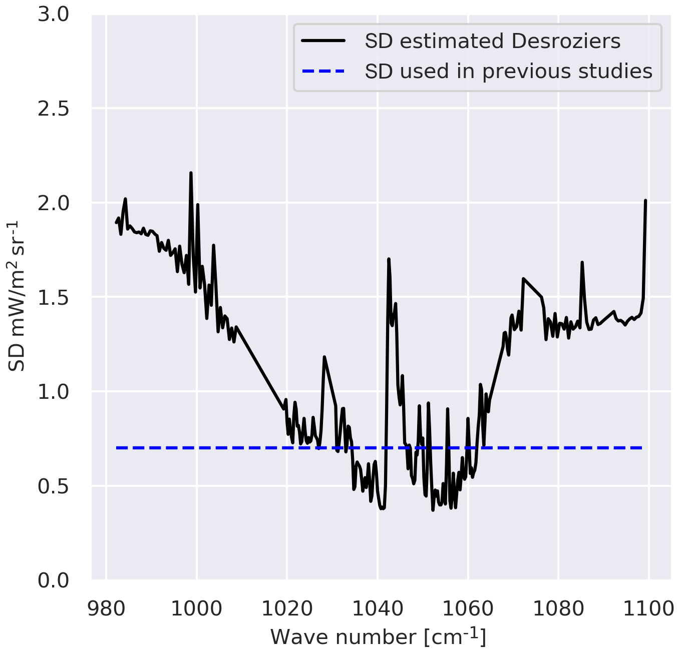
Figure 1 Standard deviation estimated using the Desroziers method (solid black line) and that used in the previous studies (blue dotted line) (Emili et al., 2019).

The IASI instrumental error is provided by the CNES (Centre National d'Etudes Spatiales), taking into account different known effects such as flight homogeneity and apodization effect (Le Barbier Laura, personal communication). The instrumental error covariance matrix is computed as described in Serio et al. (2020). This error remains smaller (about 0.2 mW m⁻² sr⁻¹ cm) than that used in the previous studies (0.7 mW m⁻² sr⁻¹ cm). Then, the large estimated standard deviation noticed in our estimation might be due to the radiative transfer input error.

To investigate the off-diagonal part of R, we present the diagnosed correlation matrix in Fig. 2. The results show high correlations between the majority of the channels (larger than 0.4). In particular, a very high correlation is observed among SST-sensitive channels (around 0.9 to 1). The regions of, relatively, lower correlation (around 0.4 to 0.7) represent the ozone channel correlations and cross correlation between ozone- and SST-sensitive channels.

Figure 2 Correlation matrix estimated using the Desroziers method.

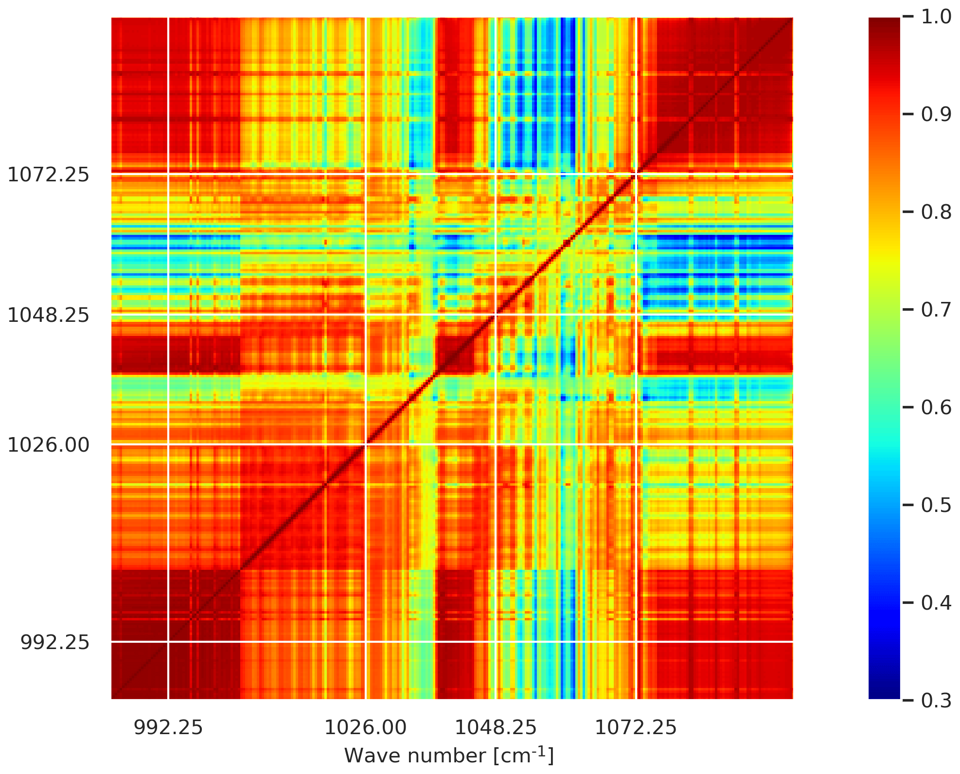
The high correlation found here was expected since previous studies have highlighted the same behaviour in this spectral region (Bormann et al., 2010; Stewart et al., 2014; Bormann et al., 2016). In fact, the use of the same radiative transfer model for all channels may introduce similar errors among these channels.

The diagnostic discussed above is based on a global estimation, without any distinction between the type of the surface (land or sea) or the time of the observation (day or night). Since the emissivity varies according to the type of the surface, and the skin temperature is strongly driven by the sun radiation, we evaluated R taking these differences into account. In terms of standard deviation, the error over land reveals large values for the SST-sensitive channels in comparison with that estimated over the sea which, in turn, reproduces a slightly different error in comparison with the global estimation (not shown). The two surfaces also introduce a slightly different error regarding the ozone band. The same behaviour as the global estimation is reproduced when the statistics were performed from the data measured separately from the day and from the night. The variability in terms of correlations is more pronounced when the surface type is considered than in the case of the observation time. The difference between the correlations estimated using all observations and pixels over the sea surface varies between 0 % and 40 % for the majority of the channels with values that can reach 60 %. These differences are located around 1035 and 1060 cm⁻¹, which correspond to the regions of low correlations (not shown).

The separate treatment of land–sea covariance matrices did not yield significant differences in terms of assimilation results compared with the use of global estimation. Hence, we have adopted the global estimation in our study. The rationale for this choice will be given during the discussion of the validation results (Sect. 5.2).

4 Assimilation results

4.1 Ozone fields

In this section, we discuss the impact of the observation-error covariances estimated previously on the ozone analysis. To this end, three experiments for the month of July 2010 were carried out:

• (i.) model run without data assimilation hereafter called the free run (or Control), and denoted in the rest of this paper as ControlExp;

• (ii.) 3D-Var assimilation of IASI radiances using a diagonal observation-error covariance matrix (as in Emili et al. (2019)), referred to here as RdiagExp;

• (iii.) 3D-Var assimilation of IASI radiances using a full matrix estimated with the Desroziers diagnostic denoted hereafter as RfullExp.

The first experiment (ControlExp) was run to evaluate the benefit of the assimilation experiments and to quantify the improvements of each of the two analyses when they are validated against independent data. The same setup of Emili et al. (2019) was adopted for RdiagExp, which was taken as a reference to characterize the impact of accounting for the estimated R in the third simulation (RfullExp).

Figure 3 shows the difference between the zonal average of the ozone analysis from the two assimilation experiments in units of parts per billion volume (ppbv). The zonal values were averaged over the month of the study before performing the difference. The impact of the estimated R varies with latitude. It also varies with the height, adding or reducing the amount of ozone. Overall, the estimated R reduces the amount of ozone in the high latitudes of the free troposphere and the tropical high stratosphere, whereas the amount is increased in the vicinity of the lower stratosphere. The maximum reduction of ozone is larger than the amount added. The amount of ozone reduction reaches 600 ppbv, whereas the increase does not exceed 300 ppbv. In high northern latitudes (30–90^∘ N), a significant addition is found (300 ppbv) covering almost the whole stratosphere, in opposition to the other latitudes where the difference changes sign with altitude. On the other hand, a large reduction of ozone is observed in the tropics at 20 hPa (more than 600 ppbv). We have performed a t test to evaluate the significance of these differences between the two experiments in terms of zonal averages. These were obtained by averaging the analysis over the month of the study and over longitudes. We have used the standard deviation computed for each average to perform our test. We have noticed that the majority of regions, especially where the differences are large (between 300 and 10 hPa), are statistically significant (not shown). To better understand the impact of the estimated R, we validate the results with independent data in the section of validation (Sect. 5).

Figure 3 The difference between the zonal average of the analysis (ppbv) from the two assimilation experiments, averaged over the month of the study (nonlinear colour map).

4.2 Surface skin temperature

The assimilated spectra include channels sensitive to both ozone and surface skin temperature. The IFS skin temperature was taken as a background in the assimilation process. We have computed the difference between the SST analysis and the background at the end of each assimilation experiment (RdiagExp and RfullExp). The skin temperature is physically linked to the ozone measured. In fact, the skin temperature interacts with the ambient atmosphere. An increase in SST can for example create a convective movement impacting the transport of the ozone. However, the skin temperature is given only at the observation location in this study, and it is specified with values interpolated from NWP forecasts (IFS), whereas ozone is a 3D field issued from the chemistry transport model. Hence, the estimation and potential account of error correlations between the two variables seem challenging in our system. In this work, we did not consider the background-error correlation that might exist between O₃ and SST.

Figure 4a shows the difference between the analysis of the SST given by RdiagExp and the IFS SST forecast, whereas Fig. 4b shows the difference between the analysis of the SST given by RfullExp and the IFS SST forecast. In terms of geographical distribution, we notice that the differences are smaller through the tropics and mid-latitudes, especially over sea, when the estimated R was adopted. Looking at the average values, RdiagExp decreases the surface skin temperature by about 0.55 ^∘C with respect to the background. The introduction of the estimated R decreases the difference between the SST analysis and that of IFS to almost −0.18 ^∘C instead of −0.55 ^∘C. The standard deviation was also reduced from 1.39 to 1.05 ^∘C. Thus, the use of the estimated R lets the SST analysis stay closer to the IFS forecasts. However, there is an increase in difference on land using RdiagExp, mainly in Africa and South America. This increase in difference over the land seems related to the dependence of observation errors on the surface. In fact, the number of observations over the sea represents almost 70 % of the total observations we have used in this study. Consequently, our SST analysis stays closer to background values (IFS forecasts) over the sea than over the land.

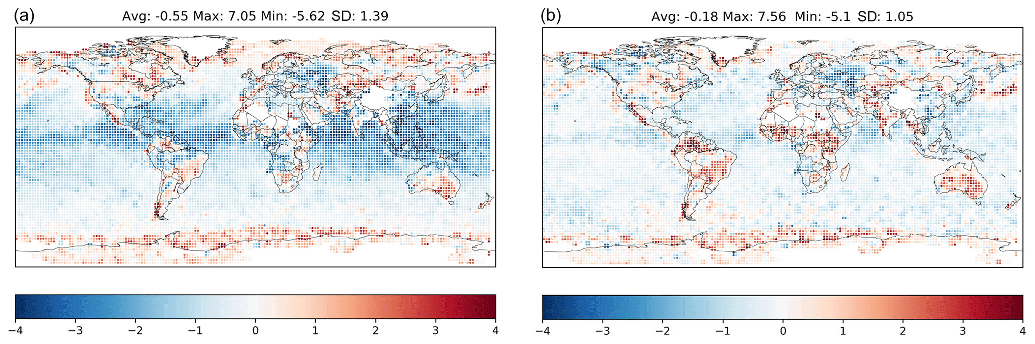
Figure 4 Difference (^∘C) between the IFS SST forecast and the analysis of the SST given by RdiagExp (with a diagonal matrix) (a) and that given by RfullExp (with a correlated matrix) (b) averaged by a box of 2^∘.

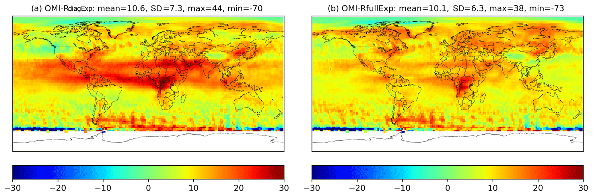
Figure 5 (a) Difference of the ozone total column (DU) provided by OMI and that of the assimilation experiment RdiagExp (b) and that of RfullExp, averaged over the month of the study.

4.3 Computational cost

In our assimilation setup, the cost function is minimized hourly. For each window, the minimizer needs to converge after a certain number of iterations. The cost of each iteration is dominated by the cost of the radiative transfer operators (tangent linear, the adjoint model) and of the background-error covariance operators. When the observation error was assumed to be uncorrelated (RdiagExp), the number of iterations needed for each hourly cycle is significantly higher than when the estimated observation-error covariance matrix is used. In fact, the introduction of the estimated R reduces the number of iterations from 150 (a fixed value to stop iterations if the convergence criteria were not attained to save computational time) to 89 iterations on average. This means that the CPU time is reduced by more than 150 % for each assimilation cycle. The convergence criteria of the BFGS algorithm are based on either the reduction of the cost function or the norm of its gradient below some given small thresholds. For the RfullExp, the convergence is achieved due to the stationarity of the cost function (first criterion). The widespread correlations (high condition number) and larger variance of the estimated R matrix lead to a downweight of the observations and are likely the reason for the improved convergence in RfullExp. This increase in the convergence speed was encountered in the Met Office 1D-Var system (Tabeart et al., 2020) where a correlated observation matrix was introduced in the system. Moreover, in Tabeart et al. (2018) the matrix R and the observation-error variance appear in the expression of the condition number of the Hessian of the variational assimilation problem, indicating that these terms are important for convergence of the minimization function.

In an attempt to distinguish the impact of the variance on the convergence speed from that of the correlations, we have performed three assimilation experiments using different R matrices. The first experiment (first experiment) employed R that was estimated from the analysis computed using a diagonal R matrix. The minimizer takes 149 iterations on average to converge (average computed for all the assimilation cycles of the month). We used the analysis given by the first experiment to estimate another R matrix. We have used this estimation to run another assimilation cycle (second experiment). We have noticed that the minimizer needs about 89 iterations on average. We have modified the R matrix of the first experiment by keeping its correlations and replacing its standard deviation with that of R used in the second experiment. The resulting matrix was used to run a third assimilation experiment. The minimizer needs about 90 iterations to converge. The results of the third experiment seem to suggest that updating the variance has a larger impact on the convergence speed.

5 Validation of O₃ analyses

5.1 Total column

Figure 5 shows the difference of the ozone total column (in Dobson units (DU)) provided by OMI and that of RdiagExp (a) and that of RfullExp (b). At first sight, we note smaller differences over the tropics between the OMI total column and the total column given by RfullExp in comparison with that given by RdiagExp. This behaviour was expected since a large reduction of the amount of ozone was observed in these regions (see Fig. 3). In the high northern latitudes, the differences were slightly increased when the estimated matrix was adopted. This is a consequence of the increase in the amount of ozone encountered in these regions in the stratosphere, compared to the amount reduced in the same region in the troposphere (Fig. 3). On the other hand, the global mean and the standard deviation of these differences are lower in the case of using the new estimated matrix (10.1 DU as a mean and 6.3 as a standard deviation when the new estimated matrix was used instead of 10.6 DU as a mean and 7.3 as a standard deviation when a diagonal matrix was used). Hence, we conclude that the estimated matrix R has slightly improved the results in terms of ozone total columns.

5.2 Vertical validation

In this section, we validate the two simulations against radiosoundings and MLS data. We use the root-mean-square error (RMSE) as the main statistical indicator to quantify the accuracy of the experiments.

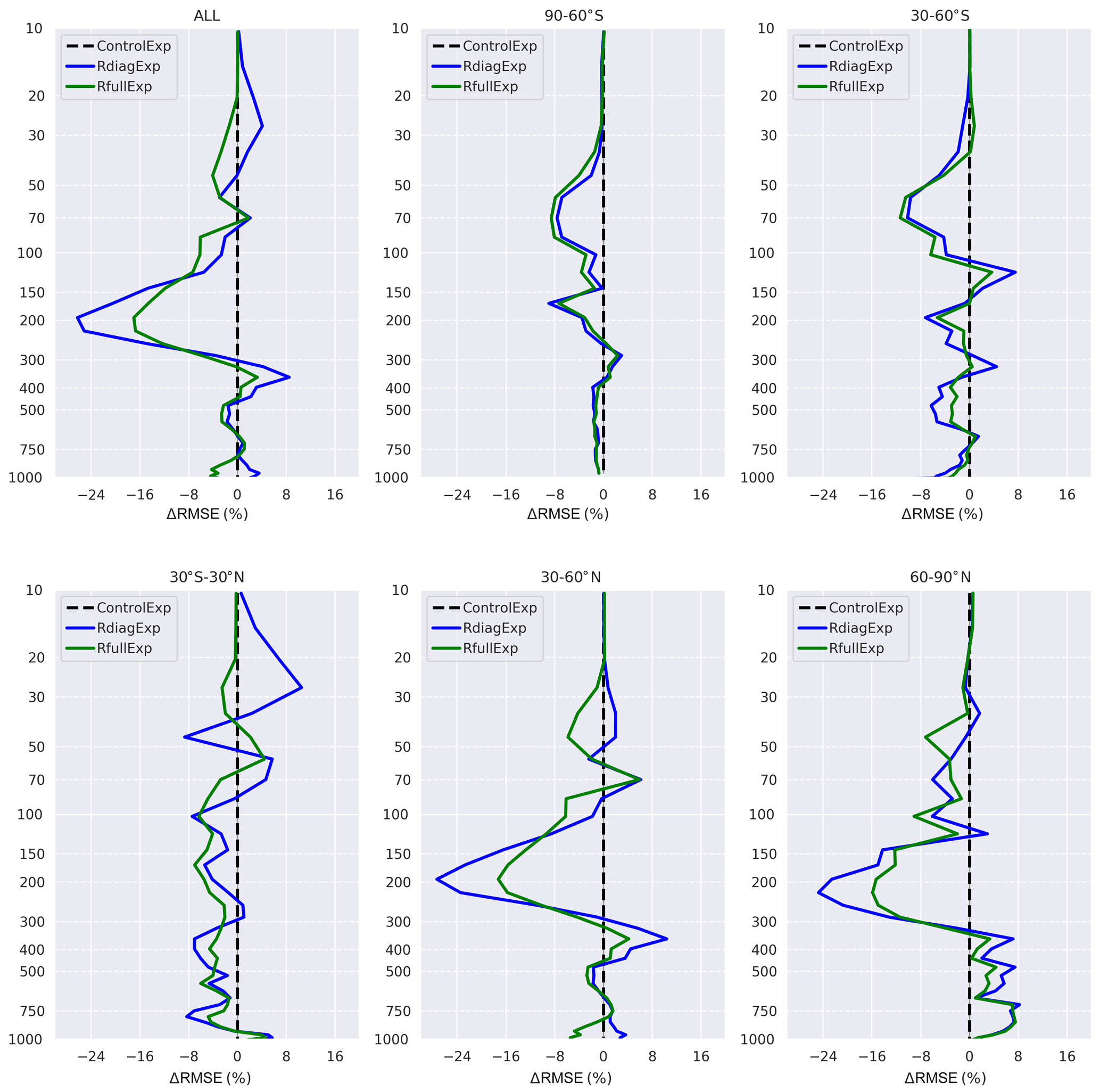
Figure 6 Normalized difference of the RMSE with respect to the ozonesondes for the R estimated (green) and R diagonal (blue). The difference of the RMSE was computed by subtracting the RMSE of the analysis from the RMSE of the control for each experiment, divided by the average profile of the ozonesondes. Negative values mean that the assimilation improved (decreased) the RMSE of the control simulation, and positive values indicate degradation (increase) of the RMSE (vertical levels are in hectopascals).

We compute the relative (to the control simulation) difference of RMSE with respect to radiosoundings and MLS averages globally and for five different latitude bands. The difference is computed by subtracting the RMSE of each experiment from that of the control simulation. Negative values indicate an improvement of the O₃ profiles. It should be noted that the representativeness of the statistics given by the MLS in the stratosphere is better than that of the radiosoundings because the number of profiles provided by MLS is much higher compared to the radiosounding ones. Consequently, higher confidence is given to the validation using the MLS data in the stratosphere.

Figure 6 reports the RMSE differences with respect to the radiosoundings. Considering the global RMSE (ALL), we notice that the experiment with the estimated matrix improves the results above 150 hPa, around 400 hPa, and near the surface. However, it also reduces the improvement from 30 % (the case of using a diagonal matrix) to 15 % in the vicinity of the upper troposphere–lower stratosphere (UTLS, 100–300 hPa).

The issue of increasing the ozone analysis errors compared to the control simulation encountered in Emili et al. (2019) is especially severe in the tropics (30^∘ S–30^∘ N). The use of the estimated R has substantially enhanced the results in this latitude band, bringing the error from +15 % to −2 %. Apart from the vicinity of 50 and 400 hPa, the results in the tropics were improved over the entire vertical profile. Regarding other latitude bands, almost the same feature of the global validation is found in the Northern Hemisphere. The two experiments show almost the same behaviour in the southern latitudes, with a slight improvement for RfullExp in the southern high latitudes (60–90^∘ S).

The MLS validation in Fig. 7 shows almost the same behaviour reported by radiosounding validation in the tropical stratosphere, where the reduction of error is remarkable. In the other latitude bands, MLS reports a similar behaviour of the two experiments, with some small differences in the Northern Hemisphere.

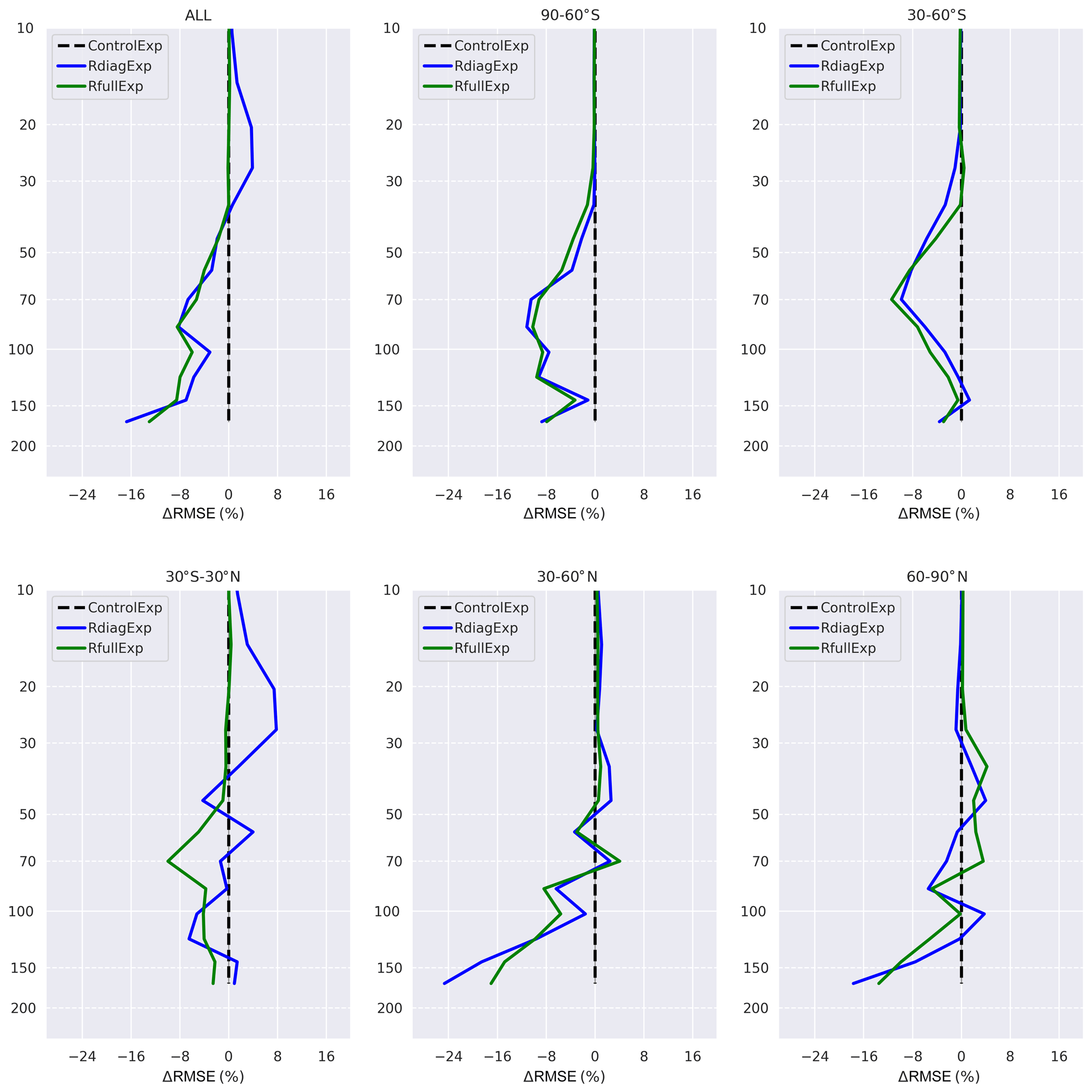
Figure 7 Normalized difference of the RMSE with respect to the MLS for the R estimated (green) and R diagonal (blue). The difference of the RMSE was computed by subtracting the RMSE of the analysis from the RMSE of the control of each experiment, divided by the average profile of the MLS. Negative values mean that the assimilation improved (decreased) the RMSE of the control simulation, and positive values indicate degradation (increase) of the RMSE. (Vertical levels are in hectopascals.)

To evaluate the significance of the differences between the analyses of the two experiments with respect to MLS and ozonesounding measurements, we have performed the t test of the differences between analyses and observations (ozonesondes then MLS). We have noticed that for the ozonesoundings, the significance differs among vertical levels. The reduction of the error between 20 and 50 hPa and between 300 and 400 hPa reported in Fig. 6 is statistically significant. For the low troposphere the differences are not significant. Unlike the ozonesounding results, the differences with respect to the MLS measurements are statistically significant for all levels discussed in MLS validation.

All things considered, the introduction of the estimated R has globally improved the O₃ profiles in the stratosphere and in the free troposphere, especially in the tropics. In spite of its degradation in the vicinity of the UTLS, the improvement always remains advantageous with respect to the control run.

The matrix used for this study (see Sect. 3.2) will now be discussed in this section since the decision was also based on the outcome of the assimilation experiments presented in this section. We sequentially performed three assimilation experiments using the first, second, and third estimations of R (Sect. 3.2). The results of validation against radiosoundings and MLS showed small differences (not shown). Therefore, to avoid the initial impact of using a diagonal matrix, we have adopted the second estimation (which uses the analyses derived from the experiment using the first estimation). In an operational framework, we may estimate the matrix daily (weekly or monthly if the period of the study is considerably long) using the analyses of the previous day (using the analysis of the previous week or month respectively). In other words, we may use a diagonal matrix to produce analyses for the first day or spin-up period, these analyses will be used to estimate the matrix that will be used for the second day, and so on throughout the period of the study.

We have also discussed the type (sea or land) and the time (day or night) of the observations while estimating the matrices. To check the impact of these differences on the assimilation results, we ran an additional assimilation experiment using the matrix estimated considering the type of the surface of each observation (since the differences were more important than if the time of the observation was considered). Only slight differences among the results have been noticed (not shown). This behaviour might be explained by the number of observations over the sea and over the land. In fact, the observations over the sea represent more than 70 % of the total observations. The differences, in terms of standard deviation, of the global estimation and that using pixels over the sea is very small in comparison with that using pixels over the land (not shown). The differences are also small in terms of correlations in the case of the sea surface in comparison with the land surface (not shown). Hence, we consider that the predominance of observations over sea averages out the potential differences caused by a separate land–sea specification of R. Thus, for simplicity, it seems reasonable to adopt the global estimation of the matrix and neglect the effect of the time and the type of the surface of the observations.

6 Conclusions

The correct specification of the observation error becomes a critical issue to efficiently assimilate the increasing amount of satellite data available in recent years. We have estimated the observation errors and their inter-channel correlations for clear-sky radiances from IASI ozone-sensitive channels. We have evaluated, then, the impact of the estimated R on the SST and ozone analysis within our 3D-Var assimilation system. The outcome has been compared with an assimilation experiment where the observation-error covariance matrix was assumed to be diagonal and the standard deviation assigned empirically like in previous studies. The results of the experiments were, then, validated against independent data: OMI, MLS, and ozonesondes.

The Desroziers diagnostics were adopted here to estimate R. The diagnostics used the analyses derived from a variational data assimilation experiment. The results have shown high correlations between the majority of the IASI spectral channels, particularly among the SST sensitive channels.

Significant differences between the results of the experiments were encountered. The introduction of the estimated R reduces the amount of ozone in the free troposphere and in the high tropical stratosphere, whereas ozone is added in the vicinity of the lower stratosphere. A validation against OMI has shown that the results were closer to the observations when the estimated matrix was adopted.

The validation against MLS and ozonesondes showed that the introduction of the estimated R has globally improved the results in the stratosphere, especially in the tropics. In spite of a slight reduction in accuracy in the vicinity of the UTLS, the improvement always remains advantageous with respect to the reference assimilation. Concerning the computational cost, the introduction of the estimated R significantly reduces the number of iterations needed for the minimizer to converge.

In summary, accounting for an estimated R significantly improves the ozone assimilation results. This approach might be adopted in the assimilation of other chemical species and also in level 2 O₃ retrievals.

In this study, the estimation was computed without taking into account any distinction of the error sources and assuming that the observation error was unbiased. More efforts will be needed to tackle these points. It should also be noted that we kept the same experiment setup of Emili et al. (2019) in order to be able to exclusively quantify the impact of the R. The background-error matrix was still defined using a relatively simple and empirical method. Further research might be needed to perform a better estimation of the background error. A new channel selection might also be performed to reduce the computational cost and the information redundancy of the IASI spectrum. On the other hand, all the experiments are performed in the context where aerosols are neglected and over 1 month. Including modelled aerosols within the radiative transfer may bring some improvements to the analyses. These aspects will be covered in future research.